On the Convergence Time of Dual Subgradient Methods for Strongly Convex Programs

Abstract

This paper studies the convergence time of dual gradient methods for general (possibly non-differentiable) strongly convex programs. For general convex programs, the convergence time of dual subgradient/gradient methods with simple running averages (running averages started from iteration $0$) is known to be $O(\frac{1}{\epsilon^{2}})$. This paper shows that the convergence time for general strongly convex programs is $O(\frac{1}{\epsilon})$. This paper also considers a variation of the average scheme, called the sliding running averages, and shows that if the dual function of the strongly convex program is locally quadratic (Note that the locally quadratic property is implied by the locally strongly concave property.) then the convergence time of the dual gradient method with sliding running averages is $O(\log(\frac{1}{\epsilon}))$. The convergence time analysis is further verified by numerical experiments.

I Introduction

Consider the following strongly convex program:

$$\min\quad f(\mathbf{x})$$ (1)

s.t. $$g_{k}(\mathbf{x})\leq 0,\forall k\in\{1,2,\ldots,m\}$$ (2)

$$\mathbf{x}\in\mathcal{X}$$ (3)

where set $\mathcal{X}\subseteq{R}^{n}$ is closed and convex; function $f(\mathbf{x})$ is continuous and strongly convex on $\mathcal{X}$ (strong convexity is defined in Section II-A); functions $g_{k}(\mathbf{x}),\forall k\in\{1,2,\ldots,m\}$ are Lipschitz continuous and convex on $\mathcal{X}$. Note that the functions $f(\mathbf{x}),g_{1}(\mathbf{x}),\ldots,g_{m}(\mathbf{x})$ are not necessarily differentiable. It is assumed throughout that problem (1)-(3) has an optimal solution. Strong convexity of $f$ implies the optimum is unique.

Convex program (1)-(3) arises often in control applications such as model predictive control (MPC) [2], decentralized multi-agent control [3], and network flow control [4, 5]. More specifically, the model predictive control problem is to solve problem (1)-(3) where $f(\mathbf{x})$ is a quadratic function and each $g_{k}(\mathbf{x})$ is a linear function [2]. In decentralized multi-agent control [3], our goal is to develop distributive algorithms to solve problem (1)-(3) where $f(\mathbf{x})$ is the sum utility of individual agents and constraints $g_{k}(\mathbf{x})\leq 0$ capture the communication or resource allocation constraints among individual agents. The network flow control and “TCP” protocols in computer networks can be interpreted as the dual subgradient algorithm for solving a problem of the form (1)-(3) [4, 5]. In particular, Section V-B shows that the dual subgradient method based online flow control rapidly converges to optimality when utilities are strongly convex.

I-A The $\epsilon$-Approximate Solution

Definition 1.

Let $\mathbf{x}^{\ast}$ be the optimal solution to problem (1)-(3). For any $\epsilon>0$, a point $\mathbf{x}^{\epsilon}\in\mathcal{X}$ is said to be an $\epsilon$-approximate solution if $f(\mathbf{x}^{\epsilon})\leq f(\mathbf{x}^{\ast})+\epsilon$ and $g_{k}(\mathbf{x}^{\epsilon})\leq\epsilon,\forall k\in\{1,\ldots,m\}$.

Definition 2.

Let $\mathbf{x}(t),t\in\{1,2,\ldots\}$ be the solution sequence yielded by an iterative algorithm. The convergence time (to an $\epsilon$ approximate solution) is the number of iterations required to achieve an $\epsilon$ approximate solution. That is, this algorithm is said to have convergence time $O(h(\epsilon))$ if $\{\mathbf{x}(t),t\geq O(h(\epsilon))\}$ is a sequence of $\epsilon$-approximate solutions.

Note if $\mathbf{x}(t)$ satisfies $f(\mathbf{x}(t))\leq f(\mathbf{x}^{\ast})+\frac{1}{t}$ and $g_{k}(\mathbf{x}(t))\leq\frac{1}{t},\forall k\in\{1,\ldots,m\}$ for all $t\geq 1$, then error decays with time like $O(\frac{1}{t})$ and the convergence time is $O(\frac{1}{\epsilon})$.

I-B The Dual Subgradient/Gradient Method

The dual subgradient method is a conventional method to solve (1)-(3) [6, 7]. It is an iterative algorithm that, every iteration, removes the inequality constraints (2) and chooses primal variables to minimize a function over the set $\mathcal{X}$. This can be decomposed into parallel smaller problems if the objective and constraint functions are separable. The dual subgradient method can be interpreted as a subgradient/gradient method applied to the Lagrangian dual function of convex program (1)-(3) and allows for many different step size rules [7]. This paper focuses on a constant step size due to its simplicity for practical implementations. Note that by Danskin’s theorem (Proposition B.25(a) in [7]), the Lagrangian dual function of a strongly convex program is differentiable, thus the dual subgradient method for strongly convex program (1)-(3) is in fact a dual gradient method. The constant step size dual subgradient/gradient method solves problem (1)-(3) as follows:

Algorithm 1.

[The Dual Subgradient/Gradient Method] Let $c>0$ be a constant step size. Let $\boldsymbol{\lambda}(0)\geq\mathbf{0},$ be a given constant vector. At each iteration $t$, update $\mathbf{x}(t)$ and $\boldsymbol{\lambda}(t+1)$ as follows:

• $\mathbf{x}(t)=\operatorname*{argmin}\limits_{\mathbf{x}\in\mathcal{X}}\left[f(\mathbf{x})+\sum_{k=1}^{m}\lambda_{k}(t)g_{k}(\mathbf{x})\right].$

• $\lambda_{k}(t+1)=\max\left\{\lambda_{k}(t)+cg_{k}(\mathbf{x}(t)),0\right\},\forall k.$

Rather than using $\mathbf{x}(t)$ from Algorithm 1 as the primal solutions, the following running average schemes are considered:

1. Simple Running Averages: Use $\overline{\mathbf{x}}(t)=\frac{1}{t}\sum_{\tau=0}^{t-1}\mathbf{x}(\tau)$ as the solution at each iteration $t\in\{1,2,\ldots\}$.

2. Sliding Running Averages: Use $\widetilde{\mathbf{x}}(t)=\mathbf{x}(0)$ and

   $$\widetilde{\mathbf{x}}(t)=\left\{\begin{array}[]{lc}\frac{1}{\frac{t}{2}}\sum_{\tau=\frac{t}{2}}^{t-1}\mathbf{x}(\tau)&~{}\text{if}~{}t~{}\text{is even}\\ \widetilde{\mathbf{x}}(t-1)&~{}\text{if}~{}t~{}\text{is odd}\end{array}\right.$$

   as the solution at each iteration $t\in\{1,2,\ldots\}$.

The simple running average sequence $\overline{\mathbf{x}}(t)$ is also called the ergodic sequence in [8]. The idea of using the running average $\overline{\mathbf{x}}(t)$ as the solutions, rather than the original primal variables $\mathbf{x}(t)$, dates back to Shor [9] and has been further developed in [10] and [8]. The constant step size dual subgradient algorithm with simple running averages is also a special case of the drift-plus-penalty algorithm, which was originally developed to solve more general stochastic optimization [11] and used for deterministic convex programs in [12]. (See Section I.C in [1] for more discussions.) This paper proposes a new running average scheme, called sliding running averages. This paper shows that the sliding running averages can have better convergence time when the dual function of the convex program satisfies additional assumptions.

I-C Related Work

A lot of literature focuses on the convergence time of dual subgradient methods to an $\epsilon$-approximiate solution. For general convex programs in the form of (1)-(3), where the objective function$f(\mathbf{x})$ is convex but not necessarily strongly convex, the convergence time of the drift-plus-penalty algorithm is shown to be $O(\frac{1}{\epsilon^{2}})$ in [12, 13]. A similar $O(\frac{1}{\epsilon^{2}})$ convergence time of the dual subgradient algorithm with the averaged primal sequence is shown in [14]. A recent work [15] shows that the convergence time of the drift-plus-penalty algorithm is $O(\frac{1}{\epsilon})$ if the dual function is locally polyhedral and the convergence time is $O(\frac{1}{\epsilon^{3/2}})$ if the dual function is locally quadratic. For a special class of strongly convex programs in the form of (1)-(3), where $f(\mathbf{x})$ is second-order differentiable and strongly convex and $g_{k}(\mathbf{x}),\forall k\in\{1,2,\ldots,m\}$ are second-order differentiable and have bounded Jacobians, the convergence time of the dual subgradient algorithm is shown to be $O(\frac{1}{\epsilon})$ in [2].

Note that convex program (1)-(3) with second order differentiable $f(\mathbf{x})$ and $g_{k}(\mathbf{x}),k\in\{1,2,\ldots,m\}$ in general can be solved via interior point methods with linear convergence time. However, to achieve good convergence time in practice, the barrier parameters must be scaled carefully and the computation complexity associated with each iteration can be high. In contrast, the dual subgradient algorithm is a Lagrangian dual method and can yield distributed implementations with low computation complexity when the objective and constraint functions are separable.

This paper considers a class of strongly convex programs that is more general than those treated in [2]. Besides the strong convexity of $f(\mathbf{x})$, we only require the constraint functions $g_{k}(\mathbf{x})$ to be Lipschitz continuous. The functions $f(\mathbf{x})$ and $g_{k}(\mathbf{x})$ can even be non-differentiable. Thus, this paper can deal with non-smooth optimization. For example, the $l_{1}$ norm $\|\mathbf{x}\|_{1}$ is non-differentiable and often appears as part of the objective or constraint functions in machine learning, compressed sensing and image processing applications. This paper shows that the convergence time of the dual subgradient method with simple running averages for general strongly convex programs is $O(\frac{1}{\epsilon})$ and the convergence time can be improved to $O(\log(\frac{1}{\epsilon}))$ by using sliding running averages when the dual function is locally quadratic.

A closely related recent work is [16] that considers strongly convex programs with strongly convex and second order differentiable objective functions $f(\mathbf{x})$ and conic constraints in the form of $\mathbf{G}\mathbf{x}+h\in\mathcal{K}$, where $\mathcal{K}$ is a proper cone. The authors in [16] show that a hybrid algorithm using both dual subgradient and dual fast gradient methods can have convergence time $O(\frac{1}{\epsilon^{2/3}})$; and the dual subgradient method can have convergence time $O(\log(\frac{1}{\epsilon}))$ if the strongly convex program satisfies an error bound property. Results in the current paper are developed independently and consider general nonlinear convex constraint functions; and show that the dual subgradient/gradient method with a different averaging scheme has an $O(\log(\frac{1}{\epsilon}))$ convergence time when the dual function is locally quadratic. Another independent parallel work is [17] that considers strongly convex programs with strongly convex and smooth objective functions $f(\mathbf{x})$ and general constraint functions $\mathbf{g}(\mathbf{x})$ with bounded Jacobians. The authors in [17] shows that the dual subgradient/gradient method with simple running averages has $O(\frac{1}{\epsilon})$ convergence.

This paper and independent parallel works [16, 17] obtain similar convergence times of the dual subgradient/gradient method with different averaging schemes for strongly convex programs under slightly different assumptions. However, the proof technique in this paper is fundamentally different from that used in [16] and [17]. Works [16, 17] and other previous works, e.g., [2], follow the classical optimization analysis approach based on the descent lemma, while this paper is based on the drift-plus-penalty analysis that was originally developed for stochastic optimization in dynamic queuing systems [18, 11]. Using the drift-plus-penalty technique, we further propose a new Lagrangian dual type algorithm with $O(\frac{1}{\epsilon})$ convergence for general convex programs (possibly without strong convexity) in a following work [19].

I-D Notations

Denote the $i$-th element of vector $\mathbf{x}\in\mathbb{R}^{n}$ as $x_{i}$. Denote $\mathbb{R}^{n}_{+}=\big{\{}\mathbf{x}\in\mathbb{R}^{n}:x_{i}\geq 0,\forall i\in\{1,\ldots,n\}\big{\}}$. For all $\mathbf{x},\mathbf{y}\in\mathbb{R}^{n}$, we write $\mathbf{x}\geq\mathbf{y}$ if and only if $x_{i}\geq y_{i},\forall 1\leq i\leq n$. Denote the Euclidean norm of vector $\mathbf{x}=[x_{1},x_{2},\ldots,x_{n}]^{T}\in\mathbb{R}^{n}$ as $\|\mathbf{x}\|=\sqrt{\sum_{i=1}^{n}x_{i}^{2}}$. For real numbers $a,b\in\mathbb{R}$ such that $a\leq b$, the projection operator onto the interval $[a,b]$ is denoted as

$$[x]_{a}^{b}=\left\{\begin{array}[]{cl}b&\text{if}~{}x>b\\ x&\text{if}~{}a\leq x\leq b\\ a&\text{if}~{}x<a\end{array}\right..$$

For a convex function $f(\mathbf{x})$, the set of all subgradients of $f$ at point $\mathbf{x}=\mathbf{x}^{\ast}$ is denoted as $\partial f(\mathbf{x}^{\ast})$; the gradient of $f$ at $\mathbf{x}=\mathbf{x}^{\ast}$ is denoted as $\nabla_{\mathbf{x}}f(\mathbf{x}^{\ast})$ if $f$ is differentiable; and the Hessian of $f$ at $\mathbf{x}=\mathbf{x}^{\ast}$ is denoted as $\nabla_{\mathbf{x}}^{2}f(\mathbf{x}^{\ast})$ if $f$ is second order differentiable. For all $x\in\mathbb{R}$, the largest integer less than or equal to $x$ is denoted as $\lfloor x\rfloor$ and the smallest integer larger than or equal to $x$ is denoted as $\lceil x\rceil$. If a square matrix $\mathbf{A}$ is positive definite, we write $A\succ 0$; and if $A$ is negative definite, we write $A\prec 0$. The $n\times n$ identity matrix is denoted as $\mathbf{I}_{n}$.

II Preliminaries and Basic Analysis

This section presents useful preliminaries in convex analysis and important facts of the dual subgradient/gradient method.

II-A Preliminaries

Definition 3 (Lipschitz Continuity).

Let $\mathcal{X}\subseteq\mathbb{R}^{n}$ be a convex set. Function $h:\mathcal{X}\rightarrow\mathbb{R}^{m}$ is said to be Lipschitz continuous on $\mathcal{X}$ with modulus $L$ if there exists $L>0$ such that $\|h(\mathbf{y})-h(\mathbf{x})\|\leq L\|\mathbf{y}-\mathbf{x}\|$ for all $\mathbf{x},\mathbf{y}\in\mathcal{X}$.

Definition 4 (Strongly Convex Functions).

Let $\mathcal{X}\subseteq\mathbb{R}^{n}$ be a convex set. Function $h$ is said to be strongly convex on $\mathcal{X}$ with modulus $\alpha$ if there exists a constant $\alpha>0$ such that $h(\mathbf{x})-\frac{1}{2}\alpha\|\mathbf{x}\|^{2}$ is convex on $\mathcal{X}$.

Lemma 1 (Theorem 6.1.2 in [20]).

Let $f(\mathbf{x})$ be strongly convex on $\mathcal{X}$ with modulus $\alpha$. Then $f(\mathbf{y})\geq f(\mathbf{x})+\mathbf{d}^{T}(\mathbf{y}-\mathbf{x})+\frac{\alpha}{2}\|\mathbf{y}-\mathbf{x}\|^{2}$ for all $\mathbf{x},\mathbf{y}\in\mathcal{X}$ and all $\mathbf{d}\in\partial f(\mathbf{x})$.

Lemma 2 (Proposition B.24 (f) in [7]).

Let $\mathcal{X}\subseteq\mathbb{R}^{n}$ be a convex set. Let function $h$ be convex on $\mathcal{X}$ and and $\mathbf{x}^{opt}$ is a global minimum of $h$ on $\mathcal{X}$. Then there exists $\mathbf{d}\in\partial f(\mathbf{x}^{opt})$ such that $\mathbf{d}^{T}(\mathbf{y}-\mathbf{x}^{opt})\geq 0$ for all $\mathbf{y}\in\mathcal{X}$.

Combining Lemma 1 and Lemma 2 gives the following:

Corollary 1.

Let $h(\mathbf{x})$ be strongly convex on convex set $\mathcal{X}$ with modulus $\alpha$. If $\mathbf{x}^{opt}$ is a global minimum, then $h(\mathbf{x}^{opt})\leq h(\mathbf{y})-\frac{\alpha}{2}\|\mathbf{y}-\mathbf{x}^{opt}\|^{2},\forall\mathbf{y}\in\mathcal{X}$.

Proof:

Fix $\mathbf{y}\in\mathcal{X}$. By Lemma 2, there exists $\mathbf{d}\in\partial h(\mathbf{x}^{opt})$ such that $\mathbf{d}^{T}(\mathbf{y}-\mathbf{x}^{opt})\geq 0$. By Lemma 1, we also have

$$h(\mathbf{y}) \geq h(\mathbf{x}^{opt})+\mathbf{d}^{T}(\mathbf{y}-\mathbf{x}^{opt})+\frac{\alpha}{2}\|\mathbf{y}-\mathbf{x}^{opt}\|^{2}$$

$$\overset{(a)}{\geq}h(\mathbf{x}^{opt})+\frac{\alpha}{2}\|\mathbf{y}-\mathbf{x}^{opt}\|^{2},$$

where $(a)$ follows from the fact that $\mathbf{d}^{T}(\mathbf{y}-\mathbf{x}^{opt})\geq 0$. ∎

II-B Assumptions

Denote the stacked vector of multiple functions $g_{1}(\mathbf{x}),g_{2}(\mathbf{x}),\ldots,g_{m}(\mathbf{x})$ as

$$\mathbf{g}(\mathbf{x})=\big{[}g_{1}(\mathbf{x}),g_{2}(\mathbf{x}),\ldots,g_{m}(\mathbf{x})\big{]}^{T}.$$

Throughout this paper, the following assumptions are imposed on convex program (1)-(3).

Assumption 1.

In convex program (1)-(3), function $f(\mathbf{x})$ is strongly convex on $\mathcal{X}$ with modulus $\alpha$; and function $\mathbf{g}(\mathbf{x})$ is Lipschitz continuous on $\mathcal{X}$ with modulus $\beta$.

Assumption 2 (Existence of Lagrange Multipliers).

There exists a Lagrange multiplier vector $\boldsymbol{\lambda}^{\ast}=[\lambda_{1}^{\ast},\lambda_{2}^{\ast},\ldots,\lambda_{m}^{\ast}]\geq\mathbf{0}$ attaining the strong duality for convex program (1)-(3). That is,

$$q(\boldsymbol{\lambda}^{\ast})=\min\limits_{\mathbf{x}\in\mathcal{X}}\left\{f(\mathbf{x}):g_{k}(\mathbf{x})\leq 0,\forall k\in\{1,2,\ldots,m\}\right\}$$

where $q(\boldsymbol{\lambda})=\min\limits_{\mathbf{x}\in\mathcal{X}}\{f(\mathbf{x})+\sum_{k=1}^{m}\lambda_{k}g_{k}(\mathbf{x})\}$ is the Lagrangian dual function of problem (1)-(3).

II-C Properties of the Drift

Denote $\boldsymbol{\lambda}(t)=\big{[}\lambda_{1}(t),\ldots,\lambda_{m}(t)\big{]}^{T}$. Define Lyapunov function $L(t)=\frac{1}{2}\|\boldsymbol{\lambda}(t)\|^{2}$ and drift $\Delta(t)=L(t+1)-L(t)$.

Lemma 3.

At each iteration $t$ in Algorithm 1,

$$\frac{1}{c}\Delta(t)=\boldsymbol{\lambda}^{T}(t+1)\mathbf{g}(\mathbf{x}(t))-\frac{1}{2c}\|\boldsymbol{\lambda}(t+1)-\boldsymbol{\lambda}(t)\|^{2}$$ (4)

Proof:

The update equations $\lambda_{k}(t+1)=\max\{\lambda_{k}(t)+cg_{k}(\mathbf{x}(t)),0\},\forall k\in\{1,2,\ldots,m\}$ can be rewritten as

$$\lambda_{k}(t+1)=\lambda_{k}(t)+c\tilde{g}_{k}(\mathbf{x}(t)),\forall k\in\{1,2,\ldots,m\},$$ (5)

where $\tilde{g}_{k}(\mathbf{x}(t))=\left\{\begin{array}[]{cl}g_{k}(\mathbf{x}(t)),&\text{if}~{}\lambda_{k}(t)+cg_{k}(\mathbf{x}(t))\geq 0\\ -\frac{1}{c}\lambda_{k}(t),&\text{else}\end{array}\right.$, $\forall k\in\{1,2,\ldots,m\}$.

Fix $k\in\{1,2,\ldots,m\}$. Squaring both sides of (5) and dividing by factor $2$ yields:

$$\frac{1}{2}[\lambda_{k}(t+1)]^{2}$$

$$= \frac{1}{2}[\lambda_{k}(t)]^{2}+\frac{c^{2}}{2}[\tilde{g}_{k}(\mathbf{x}(t))]^{2}+c\lambda_{k}(t)\tilde{g}_{k}(\mathbf{x}(t))$$

$$= \frac{1}{2}[\lambda_{k}(t)]^{2}+\frac{c^{2}}{2}[\tilde{g}_{k}(\mathbf{x}(t))]^{2}+c\lambda_{k}(t)g_{k}(\mathbf{x}(t))+c\lambda_{k}(t)[\tilde{g}_{k}(\mathbf{x}(t))-g_{k}(\mathbf{x}(t))]$$

$$\overset{(a)}{=} \frac{1}{2}[\lambda_{k}(t)]^{2}+\frac{c^{2}}{2}[\tilde{g}_{k}(\mathbf{x}(t))]^{2}+c\lambda_{k}(t)g_{k}(\mathbf{x}(t))-c^{2}\tilde{g}_{k}(\mathbf{x}(t))[\tilde{g}_{k}(\mathbf{x}(t))-g_{k}(\mathbf{x}(t))]$$

$$= \frac{1}{2}[\lambda_{k}(t)]^{2}-\frac{c^{2}}{2}[\tilde{g}_{k}(\mathbf{x}(t))]^{2}+c[\lambda_{k}(t)+c\tilde{g}_{k}(\mathbf{x}(t))]g_{k}(\mathbf{x}(t))$$

$$\overset{(b)}{=} \frac{1}{2}[\lambda_{k}(t)]^{2}-\frac{1}{2}[\lambda_{k}(t+1)-\lambda_{k}(t)]^{2}+c\lambda_{k}(t+1)g_{k}(\mathbf{x}(t))$$

where $(a)$ follows from $\lambda_{k}(t)[\tilde{g}_{k}(\mathbf{x}(t))-g_{k}(\mathbf{x}(t))]=-c\tilde{g}_{k}(\mathbf{x}(t))[\tilde{g}_{k}(\mathbf{x}(t))-g_{k}(\mathbf{x}(t))]$, which can be shown by considering $\tilde{g}_{k}(\mathbf{x}(t))=g_{k}(\mathbf{x}(t))$ and $\tilde{g}_{k}(\mathbf{x}(t))\neq g_{k}(\mathbf{x}(t))$, separately; and $(b)$ follows from the fact that $\lambda_{k}(t+1)=\lambda_{k}(t)+c\tilde{g}_{k}(\mathbf{x}(t))$. Summing over $k\in\{1,2,\ldots,m\}$ yields $\frac{1}{2}\|\boldsymbol{\lambda}(t+1)\|^{2}=\frac{1}{2}\|\boldsymbol{\lambda}(t)\|^{2}-\frac{1}{2}c^{2}\|\boldsymbol{\lambda}(t+1)-\boldsymbol{\lambda}(t)\|^{2}+c\boldsymbol{\lambda}^{T}(t+1)\mathbf{g}(\mathbf{x}(t))$. Rearranging the terms and dividing both sides by factor $c$ yields the result.

∎

III Convergence Time Analysis

This section analyzes the convergence time of Algorithm 1 for strongly convex program (1)-(3).

III-A Objective Value Violations

Lemma 4.

Let $\mathbf{x}^{\ast}\in\mathcal{X}$ be the optimal solution to problem (1)-(3). At each iteration $t$ in Algorithm 1, we have

$$\frac{1}{c}\Delta(t)+f(\mathbf{x}(t))\leq f(\mathbf{x}^{\ast}),\forall t\geq 0,$$ (6)

Proof:

Fix $t\geq 0$. Since $f(\mathbf{x})$ is strongly convex with modulus $\alpha$; $g_{k}(\mathbf{x}),\forall k\in\{1,2,\ldots,m\}$ are convex; and $\lambda_{k}(t),\forall k\in\{1,2,\ldots,m\}$ are non-negative at each iteration $t$, the function $f(\mathbf{x})+\sum_{k=1}^{m}\lambda_{k}(t)g_{k}(\mathbf{x})$ is also strongly convex with modulus $\alpha$ at each iteration $t$. Note that $\mathbf{x}(t)=\operatorname*{argmin}\limits_{\mathbf{x}\in\mathcal{X}}\Big{[}f(\mathbf{x})+\sum_{k=1}^{m}\lambda_{k}(t)g_{k}(\mathbf{x})\Big{]}$. By Corollary 1 with $\mathbf{x}^{opt}=\mathbf{x}(t)$ and $\mathbf{y}=\mathbf{x}^{\ast}$, we have

$$\big{[}f(\mathbf{x}(t))+\sum_{k=1}^{m}\lambda_{k}(t)g_{k}(\mathbf{x}(t))\big{]}\leq\big{[}f(\mathbf{x}^{\ast})+\sum_{k=1}^{m}\lambda_{k}(t)g_{k}(\mathbf{x}^{\ast})\big{]}-\frac{\alpha}{2}\|\mathbf{x}(t)-\mathbf{x}^{\ast}\|^{2}.$$

Hence, $f(\mathbf{x}(t))\leq f(\mathbf{x}^{\ast})+\mathbf{\lambda}^{T}(t)\big{[}\mathbf{g}(\mathbf{x}^{\ast})-\mathbf{g}(\mathbf{x}(t))\big{]}-\frac{\alpha}{2}\|\mathbf{x}(t)-\mathbf{x}^{\ast}\|^{2}$. Adding this inequality to equation (4) yields

$$\frac{1}{c}\Delta(t)+f(\mathbf{x}(t))$$

$$\leq f(\mathbf{x}^{\ast})-\frac{1}{2c}\|\boldsymbol{\lambda}(t+1)-\boldsymbol{\lambda}(t)\|^{2}-\frac{\alpha}{2}\|\mathbf{x}(t)-\mathbf{x}^{\ast}\|^{2}+\boldsymbol{\lambda}^{T}(t)[\mathbf{g}(\mathbf{x}^{\ast})-\mathbf{g}(\mathbf{x}(t))]+\boldsymbol{\lambda}^{T}(t+1)\mathbf{g}(\mathbf{x}(t)).$$

Define

$$B(t)=-\frac{1}{2c}\|\boldsymbol{\lambda}(t+1)-\boldsymbol{\lambda}(t)\|^{2}-\frac{\alpha}{2}\|\mathbf{x}(t)-\mathbf{x}^{\ast}\|^{2}+\boldsymbol{\lambda}^{T}(t)[\mathbf{g}(\mathbf{x}^{\ast})-\mathbf{g}(\mathbf{x}(t))]+\boldsymbol{\lambda}^{T}(t+1)\mathbf{g}(\mathbf{x}(t)).$$

Next, we need to show that $B(t)\leq 0$.

Since $\mathbf{x}^{\ast}$ is the optimal solution to problem (1)-(3), we have $g_{k}(\mathbf{x}^{\ast})\leq 0,\forall k\in\{1,2,\ldots,m\}$. Note that $\lambda_{k}(t+1)\geq 0,\forall k\in\{1,2,\ldots,m\},\forall t\geq 0$. Thus,

$$\boldsymbol{\lambda}^{T}(t+1)\mathbf{g}(\mathbf{x}^{\ast})\leq 0,\quad\forall t\geq 0$$ (7)

Now we have,

$$B(t)= -\frac{1}{2c}\|\boldsymbol{\lambda}(t+1)-\boldsymbol{\lambda}(t)\|^{2}-\frac{\alpha}{2}\|\mathbf{x}(t)-\mathbf{x}^{\ast}\|^{2}+\boldsymbol{\lambda}^{T}(t)[\mathbf{g}(\mathbf{x}^{\ast})-\mathbf{g}(\mathbf{x}(t))]+\boldsymbol{\lambda}^{T}(t+1)\mathbf{g}(\mathbf{x}(t))$$

$$\overset{(a)}{\leq} -\frac{1}{2c}\|\boldsymbol{\lambda}(t+1)-\boldsymbol{\lambda}(t)\|^{2}-\frac{\alpha}{2}\|\mathbf{x}(t)-\mathbf{x}^{\ast}\|^{2}+\boldsymbol{\lambda}^{T}(t)[\mathbf{g}(\mathbf{x}^{\ast})-\mathbf{g}(\mathbf{x}(t))]+\boldsymbol{\lambda}^{T}(t+1)\mathbf{g}(\mathbf{x}(t))$$

$$\quad-\boldsymbol{\lambda}^{T}(t+1)\mathbf{g}(\mathbf{x}^{\ast})$$

$$= -\frac{1}{2c}\|\boldsymbol{\lambda}(t+1)-\boldsymbol{\lambda}(t)\|^{2}-\frac{\alpha}{2}\|\mathbf{x}(t)-\mathbf{x}^{\ast}\|^{2}+[\boldsymbol{\lambda}^{T}(t)-\boldsymbol{\lambda}^{T}(t+1)][\mathbf{g}(\mathbf{x}^{\ast})-\mathbf{g}(\mathbf{x}(t))]$$

$$\overset{(b)}{\leq} -\frac{1}{2c}\|\mathbf{Q}(t+1)-\mathbf{Q}(t)\|^{2}-\frac{\alpha}{2}\|\mathbf{x}(t)-\mathbf{x}^{\ast}\|^{2}+\|\boldsymbol{\lambda}(t)-\boldsymbol{\lambda}(t+1)\|\|\mathbf{g}(\mathbf{x}(t))-\mathbf{g}(\mathbf{x}^{\ast})\|$$

$$\overset{(c)}{\leq} -\frac{1}{2c}\|\boldsymbol{\lambda}(t+1)-\boldsymbol{\lambda}(t)\|^{2}-\frac{\alpha}{2}\|\mathbf{x}(t)-\mathbf{x}^{\ast}\|^{2}+\beta\|\boldsymbol{\lambda}(t)-\boldsymbol{\lambda}(t+1)\|\|\mathbf{x}(t)-\mathbf{x}^{\ast}\|$$

$$= -\frac{1}{2c}\Big{(}\|\boldsymbol{\lambda}(t+1)-\boldsymbol{\lambda}(t)\|-c\beta\|\mathbf{x}(t)-\mathbf{x}^{\ast}\|\Big{)}^{2}-\frac{1}{2}(\alpha-c\beta^{2})\|\mathbf{x}(t)-\mathbf{x}^{\ast}\|^{2}$$

$$\overset{(d)}{\leq} 0$$

where $(a)$ follows from (7); $(b)$ follows from the Cauchy-Schwarz inequality; $(c)$ follows from Assumption 1; and $(d)$ follows from $c\leq\frac{\alpha}{\beta^{2}}$. ∎

Theorem 1 (Objective Value Violations).

Let $\mathbf{x}^{\ast}\in\mathcal{X}$ be the optimal solution to problem (1)-(3). If $c\leq\frac{\alpha}{\beta^{2}}$ in Algorithm 1, then

$$f(\overline{\mathbf{x}}(t))\leq f(\mathbf{x}^{\ast})+\frac{\|\boldsymbol{\lambda}(0)\|^{2}}{2ct},\forall t\geq 1.$$

Proof:

By Lemma 4, we have $\frac{1}{c}\Delta(\tau)+f(\mathbf{x}(\tau))\leq f(\mathbf{x}^{\ast})$ for all $\tau\in\{0,1,\ldots,t-1\}$. Summing over $\tau\in\{0,1,\ldots,t-1\}$ we have:

$$\frac{1}{c}\sum_{\tau=0}^{t-1}\Delta(\tau)+\sum_{\tau=0}^{t-1}f(\mathbf{x}(\tau))\leq tf(\mathbf{x}^{\ast})$$

$$\Rightarrow\quad \frac{1}{c}[L(t)-L(0)]+\sum_{\tau=0}^{t-1}f(\mathbf{x}(\tau))\leq tf(\mathbf{x}^{\ast})$$

$$\Rightarrow\quad \frac{1}{t}\sum_{\tau=0}^{t-1}f(\mathbf{x}(\tau))\leq f(\mathbf{x}^{\ast})+\frac{L(0)-L(t)}{ct}\leq f(\mathbf{x}^{\ast})+\frac{L(0)}{ct}$$

Note that $\overline{\mathbf{x}}(t)=\frac{1}{t}\sum_{\tau=0}^{t-1}\mathbf{x}(\tau)$ and by the convexity of $f(\mathbf{x})$, we have

$$f(\overline{\mathbf{x}}(t))\leq\frac{1}{t}\sum_{\tau=0}^{t-1}f(\mathbf{x}(\tau))\leq f(\mathbf{x}^{\ast})+\frac{L(0)}{ct}=f(\mathbf{x}^{\ast})+\frac{\|\boldsymbol{\lambda}(0)\|^{2}}{2ct}$$

∎

Remark 1.

Similarly, we can prove that $f(\widetilde{\mathbf{x}}(2t))\leq f(\mathbf{x}^{\ast})+\frac{\|\boldsymbol{\lambda}(t)\|^{2}}{2ct}$ since $\widetilde{\mathbf{x}}(2t)=\frac{1}{t}\sum_{\tau=t}^{2t-1}\mathbf{x}(\tau)$. A later lemma (Lemma 6) guarantees that $\|\boldsymbol{\lambda}(t)\|\leq\sqrt{\|\boldsymbol{\lambda}(0)\|^{2}+\|\boldsymbol{\lambda}^{\ast}\|^{2}}+\|\boldsymbol{\lambda}^{\ast}\|$, where $\boldsymbol{\lambda}^{\ast}$ is defined in Assumption 2. Thus, $f(\widetilde{\mathbf{x}}(2t))\leq f(\mathbf{x}^{\ast})+\frac{\big{(}\sqrt{\|\boldsymbol{\lambda}(0)\|^{2}+\|\boldsymbol{\lambda}^{\ast}\|^{2}}+\|\boldsymbol{\lambda}^{\ast}\|\big{)}^{2}}{2ct},\forall t\geq 1.$

III-B Constraint Violations

The analysis of constraint violations is similar to that in [13] for general convex programs. However, using the improved upper bound in Lemma 4, the convergence time of constraint violations in strongly convex programs is order-wise better than that in general convex programs.

Lemma 5.

For any $t_{2}>t_{1}\geq 0$, $\lambda_{k}(t_{2})\geq\lambda_{k}(t_{1})+c\displaystyle{\sum_{\tau=t_{1}}^{t_{2}-1}g_{k}(\mathbf{x}(\tau))},\forall k\in\{1,2,\ldots,m\}$. In particular, for any $t>0$, $\lambda_{k}(t)\geq\lambda_{k}(0)+c\displaystyle{\sum_{\tau=0}^{t-1}g_{k}(\mathbf{x}(\tau))},\forall k\in\{1,2,\ldots,m\}$

Proof:

Fix $k\in\{1,2,\ldots,m\}$. Note that $\lambda_{k}(t_{1}+1)=\max\{\lambda_{k}(t_{1})+cg_{k}(\mathbf{x}(t_{1})),0\}\geq\lambda_{k}(t_{1})+cg_{k}(\mathbf{x}(t_{1}))$. By induction, this lemma follows. ∎

Lemma 6.

Let $\boldsymbol{\lambda}^{\ast}\geq\mathbf{0}$ be given in Assumption 2. If $c\leq\frac{\alpha}{\beta^{2}}$ in Algorithm 1, then $\boldsymbol{\lambda}(t)$ satisfies

$$\|\boldsymbol{\lambda}(t)\|\leq\sqrt{\|\boldsymbol{\lambda}(0)\|^{2}+\|\boldsymbol{\lambda}^{\ast}\|^{2}}+\|\boldsymbol{\lambda}^{\ast}\|,\forall t\geq 1.$$ (8)

Proof:

Let $\mathbf{x}^{\ast}$ be the optimal solution to problem (1)-(3). AAssumption 2 implies that

$$f(\mathbf{x}^{\ast})=q(\boldsymbol{\lambda}^{\ast})\leq f(\mathbf{x}(\tau))+\sum_{k=1}^{m}\lambda_{k}^{\ast}g_{k}(\mathbf{x}(\tau)),\forall\tau\in\{0,1,\ldots\},$$

where the inequality follows from the definition of $q(\boldsymbol{\lambda})$.

Thus, we have $f(\mathbf{x}^{\ast})-f(\mathbf{x}(\tau))\leq\sum_{k=1}^{m}\lambda_{k}^{\ast}g_{k}(\mathbf{x}(\tau)),\forall\tau\in\{0,1,\ldots\}$. Summing over $\tau\in\{0,1,\ldots,t-1\}$ yields

$$tf(\mathbf{x}^{\ast})-\sum_{\tau=0}^{t-1}f(\mathbf{x}(\tau)) \leq\sum_{\tau=0}^{t-1}\sum_{k=1}^{m}\lambda_{k}^{\ast}g_{k}(\mathbf{x}(\tau))$$

$$=\sum_{k=1}^{m}\lambda_{k}^{\ast}\Big{[}\sum_{\tau=0}^{t-1}g_{k}(\mathbf{x}(\tau))\Big{]}$$

$$\overset{(a)}{\leq}\frac{1}{c}\sum_{k=1}^{m}\lambda_{k}^{\ast}[\lambda_{k}(t)-\lambda_{k}(0)]$$

$$\leq\frac{1}{c}\sum_{k=1}^{m}\lambda_{k}^{\ast}\lambda_{k}(t)$$

$$\overset{(b)}{\leq}\frac{1}{c}\|\boldsymbol{\lambda}^{\ast}\|\|\boldsymbol{\lambda}(t)\|$$ (9)

where $(a)$ follows from Lemma 5 and $(b)$ follows from the Cauchy-Schwarz inequality. On the other hand, summing (6) in Lemma 4 over $\tau\in\{0,1,\ldots,t-1\}$ yields

$$tf(\mathbf{x}^{\ast})-\sum_{\tau=0}^{t-1}f(\mathbf{x}(\tau)) \geq\frac{L(t)-L(0)}{c}$$

$$=\frac{\|\boldsymbol{\lambda}(t)\|^{2}-\|\boldsymbol{\lambda}(0)\|^{2}}{2c}$$ (10)

Combining (9) and (10) yields

$$\frac{\|\boldsymbol{\lambda}(t)\|^{2}-\|\boldsymbol{\lambda}(0)\|^{2}}{2c}\leq\frac{1}{c}\|\boldsymbol{\lambda}^{\ast}\|\|\boldsymbol{\lambda}(t)\|$$

$$\Rightarrow\quad \Big{(}\|\boldsymbol{\lambda}(t)\|-\|\boldsymbol{\lambda}^{\ast}\|\Big{)}^{2}\leq\|\boldsymbol{\lambda}(0)\|^{2}+\|\boldsymbol{\lambda}^{\ast}\|^{2}$$

$$\Rightarrow\quad \|\boldsymbol{\lambda}(t)\|\leq\sqrt{\|\boldsymbol{\lambda}(0)\|^{2}+\|\boldsymbol{\lambda}^{\ast}\|^{2}}+\|\boldsymbol{\lambda}^{\ast}\|$$

∎

Theorem 2 (Constraint Violations).

Let $\boldsymbol{\lambda}^{\ast}\geq\mathbf{0}$ be defined in Assumption 2. If $c\leq\frac{\alpha}{\beta^{2}}$ in Algorithm 1, then the constraint functions satisfy $g_{k}(\overline{\mathbf{x}}(t))\leq\frac{\sqrt{\|\boldsymbol{\lambda}(0)\|^{2}+\|\boldsymbol{\lambda}^{\ast}\|^{2}}+\|\boldsymbol{\lambda}^{\ast}\|}{ct},\forall k\in\{1,2,\ldots,m\},\forall t\geq 1$.

Proof:

Fix $t\geq 1$ and $k\in\{1,2,\ldots,m\}$. Recall that $\overline{\mathbf{x}}(t)=\frac{1}{t}\sum_{\tau=0}^{t-1}\mathbf{x}(\tau)$. Thus,

$$g_{k}(\overline{\mathbf{x}}(t)) \overset{(a)}{\leq}\frac{1}{t}\sum_{\tau=0}^{t-1}g_{k}(\mathbf{x}(\tau))$$

$$\overset{(b)}{\leq}\frac{\lambda_{k}(t)-\lambda_{k}(0)}{ct}$$

$$\leq\frac{\lambda_{k}(t)}{ct}$$

$$\leq\frac{\|\boldsymbol{\lambda}(t)\|}{ct}$$

$$\overset{(c)}{\leq}\frac{\sqrt{\|\boldsymbol{\lambda}(0)\|^{2}+\|\boldsymbol{\lambda}^{\ast}\|^{2}}+\|\boldsymbol{\lambda}^{\ast}\|}{ct}$$

where $(a)$ follows from the convexity of $g_{k}(\mathbf{x}),k\in\{1,2,\ldots,m\}$; $(b)$ follows from Lemma 5; and $(c)$ follows from Lemma 6. ∎

Remark 2.

Similarly, we can prove that $g_{k}(\widetilde{\mathbf{x}}(2t))\leq\frac{\sqrt{\|\boldsymbol{\lambda}(0)\|^{2}+\|\boldsymbol{\lambda}^{\ast}\|^{2}}+\|\boldsymbol{\lambda}^{\ast}\|}{ct},\forall k\in\{1,2,\ldots,m\},\forall t\geq 1$

The next corollary provides a lower bound of $f(\overline{\mathbf{x}}(t))$ and follows directly from strong duality for convex programs and Theorem 2.

Corollary 2.

Let $\boldsymbol{\lambda}^{\ast}\geq\mathbf{0}$ be defined in Assumption 2. If $c\leq\frac{\alpha}{\beta^{2}}$ in Algorithm 1, then $f(\overline{\mathbf{x}}(t))$ has a lower bound given by $f(\overline{\mathbf{x}}(t))\geq f(\mathbf{x}^{\ast})-\frac{1}{t}\frac{\sqrt{\|\boldsymbol{\lambda}(0)\|^{2}+\|\boldsymbol{\lambda}^{\ast}\|^{2}}+\|\boldsymbol{\lambda}^{\ast}\|}{c}\sum_{k=1}^{m}\lambda_{k}^{\ast},\forall t\geq 1$.

Proof:

Fix $t\geq 1$. By the strong duality, we have

$$f(\overline{\mathbf{x}}(t))+\sum_{k=1}^{m}\lambda_{k}^{\ast}g_{k}(\overline{\mathbf{x}}(t))\geq q(\boldsymbol{\lambda}^{\ast})=f(\mathbf{x}^{\ast})+\sum_{k=1}^{m}\lambda_{k}^{\ast}g_{k}(\mathbf{x}^{\ast})=f(\mathbf{x}^{\ast})$$

Thus, we have

$$f(\overline{\mathbf{x}}(t))\geq f(\mathbf{x}^{\ast})-\sum_{k=1}^{m}\lambda_{k}^{\ast}g_{k}(\overline{\mathbf{x}}(t))$$

$$\overset{(a)}{\geq} f(\mathbf{x}^{\ast})-\sum_{k=1}^{m}\lambda_{k}^{\ast}\frac{\sqrt{\|\boldsymbol{\lambda}(0)\|^{2}+\|\boldsymbol{\lambda}^{\ast}\|^{2}}+\|\boldsymbol{\lambda}^{\ast}\|}{ct}$$

$$= f(\mathbf{x}^{\ast})-\frac{1}{t}\frac{\sqrt{\|\boldsymbol{\lambda}(0)\|^{2}+\|\boldsymbol{\lambda}^{\ast}\|^{2}}+\|\boldsymbol{\lambda}^{\ast}\|}{c}\sum_{k=1}^{m}\lambda_{k}^{\ast}$$

where (a) follows from the constraint violation bound, i.e., Theorem 2, and the fact that $\lambda_{k}^{\ast}\geq 0,\forall k\in\{1,2,\ldots,m\}$. ∎

III-C Convergence Time of Algorithm 1

The next theorem summarizes Theorem 1 and Theorem 2.

Theorem 3.

Let $\mathbf{x}^{\ast}\in\mathcal{X}$ be the optimal solution to problem (1)-(3). Let $\boldsymbol{\lambda}^{\ast}\geq\mathbf{0}$ be given in Assumption 2. If $c\leq\frac{\alpha}{\beta^{2}}$ in Algorithm 1, then for all $t\geq 1$,

$$f(\overline{\mathbf{x}}(t))\leq f(\mathbf{x}^{\ast})+\frac{\|\boldsymbol{\lambda}(0)\|^{2}}{2ct}.$$

$$g_{k}(\overline{\mathbf{x}}(t))\leq\frac{\sqrt{\|\boldsymbol{\lambda}(0)\|^{2}+\|\boldsymbol{\lambda}^{\ast}\|^{2}}+\|\boldsymbol{\lambda}^{\ast}\|}{t},\forall k\in\{1,2,\ldots,m\}.$$

Specifically, if $\boldsymbol{\lambda}(0)=\mathbf{0}$, then

$$f(\overline{\mathbf{x}}(t))\leq f(\mathbf{x}^{\ast}).$$

$$g_{k}(\overline{\mathbf{x}}(t))\leq\frac{2\|\boldsymbol{\lambda}^{\ast}\|}{ct},\forall k\in\{1,2,\ldots,m\}.$$

In summary, if $c\leq\frac{\alpha}{\beta^{2}}$ in Algorithm 1, then $\overline{\mathbf{x}}(t)$ ensures that error decays like $O(\frac{1}{t})$ and provides an $\epsilon$-approximiate solution with convergence time $O(\frac{1}{\epsilon})$.

Remark 3.

If $c\leq\frac{\alpha}{\beta^{2}}$ in Algorithm 1, then $\widetilde{\mathbf{x}}(t)$ also ensures that error decays like $O(\frac{1}{t})$ and provides an $\epsilon$-approximiate solution with convergence time $O(\frac{1}{\epsilon})$.

IV Extensions

This section shows that the convergence time of sliding running averages $\widetilde{\mathbf{x}}(t)$ is $O(\log(\frac{1}{\epsilon}))$ when the dual function of problem (1)-(3) satisfies additional assumptions.

IV-A Smooth Dual Functions

Definition 5 (Smooth Functions).

Let $\mathcal{X}\subseteq\mathbb{R}^{n}$ and function $h(\mathbf{x})$ be continuously differentiable on $\mathcal{X}$. Function $h(\mathbf{x})$ is said to be smooth on $\mathcal{X}$ with modulus $L$ if $\nabla_{\mathbf{x}}h(\mathbf{x})$ is Lipschitz continuous on $\mathcal{X}$ with modulus $L$.

Define $q(\boldsymbol{\lambda})=\min\limits_{\mathbf{x}\in\mathcal{X}}\{f(\mathbf{x})+\boldsymbol{\lambda}^{T}\mathbf{g}(\mathbf{x})\}$ as the dual function of problem (1)-(3). Recall that $f(\mathbf{x})$ is strongly convex with modulus $\alpha$ by Assumption 1. For fixed $\boldsymbol{\lambda}\in\mathbb{R}^{m}_{+}$, $f(\mathbf{x})+\boldsymbol{\lambda}^{T}\mathbf{g}(\mathbf{x})$ is strongly convex with respect to $\mathbf{x}\in\mathcal{X}$ with modulus $\alpha$. Define $\mathbf{x}(\boldsymbol{\lambda})=\operatorname*{argmin}_{\mathbf{x}\in\mathcal{X}}\{f(\mathbf{x})+\boldsymbol{\lambda}^{T}\mathbf{g}(\mathbf{x})\}$. By Danskin’s theorem (Proposition B.25 in [7]), $q(\boldsymbol{\lambda})$ is differentiable with gradient $\nabla_{\boldsymbol{\lambda}}q(\boldsymbol{\lambda})=\mathbf{g}(\mathbf{x}(\boldsymbol{\lambda}))$.

Lemma 7 (Smooth Dual Functions).

The dual function $q(\boldsymbol{\lambda})$ is smooth on $\mathbb{R}^{m}_{+}$ with modulus $\gamma=\frac{\beta^{2}}{\alpha}$.

Proof:

Fix $\boldsymbol{\lambda},\boldsymbol{\mu}\in\mathbb{R}^{m}_{+}$. Let $\mathbf{x}(\boldsymbol{\lambda})=\operatorname*{argmin}_{\mathbf{x}\in\mathcal{X}}\{f(\mathbf{x})+\boldsymbol{\lambda}^{T}\mathbf{g}(\mathbf{x})\}$ and $\mathbf{x}(\boldsymbol{\mu})=\operatorname*{argmin}_{\mathbf{x}\in\mathcal{X}}\{f(\mathbf{x})+\boldsymbol{\mu}^{T}\mathbf{g}(\mathbf{x})\}$. By Corollary 1, we have

$$f(\mathbf{x}(\boldsymbol{\lambda}))+\boldsymbol{\lambda}^{T}\mathbf{g}(\mathbf{x}(\boldsymbol{\lambda}))\leq f(\mathbf{x}(\boldsymbol{\mu}))+\boldsymbol{\lambda}^{T}\mathbf{g}(\mathbf{x}(\boldsymbol{\mu}))-\frac{\alpha}{2}\|\mathbf{x}(\boldsymbol{\lambda})-\mathbf{x}(\boldsymbol{\mu})\|^{2}$$

$$f(\mathbf{x}(\boldsymbol{\mu}))+\boldsymbol{\mu}^{T}\mathbf{g}(\mathbf{x}(\boldsymbol{\mu}))\leq f(\mathbf{x}(\boldsymbol{\lambda}))+\boldsymbol{\mu}^{T}\mathbf{g}(\mathbf{x}(\boldsymbol{\lambda}))-\frac{\alpha}{2}\|\mathbf{x}(\boldsymbol{\lambda})-\mathbf{x}(\boldsymbol{\mu})\|^{2}$$

Summing the above two inequalities and simplifying gives

$$\alpha\|\mathbf{x}(\boldsymbol{\lambda})-\mathbf{x}(\boldsymbol{\mu})\|^{2} \leq[\boldsymbol{\mu}-\boldsymbol{\lambda}]^{T}[\mathbf{g}(\mathbf{x}(\boldsymbol{\lambda}))-\mathbf{g}(\mathbf{x}(\boldsymbol{\mu}))]$$

$$\overset{(a)}{\leq}\|\boldsymbol{\mu}-\boldsymbol{\lambda}\|\|\mathbf{g}(\mathbf{x}(\boldsymbol{\lambda}))-\mathbf{g}(\mathbf{x}(\boldsymbol{\mu}))\|$$

$$\overset{(b)}{\leq}\beta\|\boldsymbol{\mu}-\boldsymbol{\lambda}\|\|\mathbf{x}(\boldsymbol{\lambda})-\mathbf{x}(\boldsymbol{\mu})\|$$

where (a) follows from the Cauchy-Schwarz inequality and (b) follows because $\mathbf{g}(\mathbf{x})$ is Lipschitz coninuous. This implies

$$\|\mathbf{x}(\boldsymbol{\lambda})-\mathbf{x}(\boldsymbol{\mu})\|\leq\frac{\beta}{\alpha}\|\boldsymbol{\lambda}-\boldsymbol{\mu}\|$$ (11)

Thus, we have

$$\|\nabla q(\boldsymbol{\lambda})-\nabla q(\boldsymbol{\mu})\| \overset{(a)}{=}\|\mathbf{g}(\mathbf{x}(\boldsymbol{\lambda}))-\mathbf{g}(\mathbf{x}(\boldsymbol{\mu}))\|$$

$$\overset{(b)}{\leq}\beta\|\mathbf{x}(\boldsymbol{\lambda})-\mathbf{x}(\boldsymbol{\mu})\|$$

$$\overset{(c)}{\leq}\frac{\beta^{2}}{\alpha}\|\boldsymbol{\lambda}-\boldsymbol{\mu}\|$$

where (a) follows from $\nabla_{\boldsymbol{\lambda}}q(\boldsymbol{\lambda})=\mathbf{g}(\mathbf{x}(\boldsymbol{\lambda}))$; (b) follows from the Lipschitz continuity of $\mathbf{g}(\mathbf{x})$; and (c) follows from (11).

Thus, $q(\boldsymbol{\lambda})$ is smooth on $\mathbb{R}^{m}_{+}$ with modulus $L=\frac{\beta^{2}}{\alpha}$. ∎

Since $\nabla_{\boldsymbol{\lambda}}q(\boldsymbol{\lambda}(t))=\mathbf{g}(\mathbf{x}(t))$, the dynamic of $\boldsymbol{\lambda}(t)$ can be interpreted as the projected gradient method with step size $c$ to solve $\max_{\boldsymbol{\lambda}\in\mathbb{R}^{m}_{+}}\left\{q(\boldsymbol{\lambda})\right\}$ where $\mathbf{q}(\cdot)$ is a smooth function by Lemma 7. Thus, we have the next lemma.

Lemma 8.

Assume problem (1)-(3) satisfies Assumptions 1-2. If $c\leq\frac{\alpha}{\beta^{2}}$ in Algorithm 1, then

$$q(\boldsymbol{\lambda}^{\ast})-q(\boldsymbol{\lambda}(t))\leq\frac{1}{2ct}\|\boldsymbol{\lambda}(0)-\boldsymbol{\lambda}^{\ast}\|^{2},\quad\forall t\geq 1.$$

Proof:

Recall that a projected gradient descent algorithm with step size $c<\frac{1}{\gamma}$ converges to the maximum of a concave function with smooth modulus $\gamma$ with the error decaying like $O(\frac{1}{t})$. Thus, this lemma follows. The proof is essentially the same as the convergence time proof of the projected gradient method for set constrained smooth optimization in [21]. See Appendix A for the detailed proof. ∎

IV-B Convergence Time Analysis of Problems with Locally Quadratic Dual Functions

In addition to Assumptions 1-2, we further require the next assumption in this subsection.

Assumption 3 (Locally Quadratic Dual Functions).

Let $\boldsymbol{\lambda}^{\ast}$ be a Lagrange multiplier of problem (1)-(3) defined in Assumption 2. There exists $D_{q}>0$ and $L_{q}>0$, where the subscript $q$ denotes locally “quadratic”, such that for all $\boldsymbol{\lambda}\in\{\boldsymbol{\lambda}\in\mathbb{R}^{m}_{+}:\|\boldsymbol{\lambda}-\boldsymbol{\lambda}^{\ast}\|\leq D_{q}\}$, the dual function $q(\boldsymbol{\lambda})=\min\limits_{\mathbf{x}\in\mathcal{X}}\Big{\{}f(\mathbf{x})+\sum_{k=1}^{m}\lambda_{k}g_{k}(\mathbf{x})\Big{\}}$ satisfies

$$q(\boldsymbol{\lambda}^{\ast})\geq q(\boldsymbol{\lambda})+L_{q}\|\boldsymbol{\lambda}-\boldsymbol{\lambda}^{\ast}\|^{2}.$$

Lemma 9.

Suppose problem (1)-(3) satisfies Assumptions 1, 2 and 3. Let $q(\boldsymbol{\lambda}),\boldsymbol{\lambda}^{\ast},D_{q}$ and $L_{q}$ be defined in Assumption 3. We have the following properties:

1. If $\boldsymbol{\lambda}\in\mathbb{R}^{m}_{+}$ and $q(\boldsymbol{\lambda}^{\ast})-q(\boldsymbol{\lambda})\leq L_{q}D_{q}^{2}$, then $\|\boldsymbol{\lambda}-\boldsymbol{\lambda}^{\ast}\|\leq D_{q}$.

2. The Lagrange multiplier defined in Assumption 2 is unique.

Proof:

1. Assume not and there exists $\boldsymbol{\lambda}^{\prime}\in\mathbb{R}^{m}_{+}$ such that $q(\boldsymbol{\lambda}^{\ast})-q(\boldsymbol{\lambda}^{\prime})\leq L_{q}D_{q}^{2}$ and $\|\boldsymbol{\lambda}^{\prime}-\boldsymbol{\lambda}^{\ast}\|>D_{q}$. Define $\boldsymbol{\lambda}=(1-\eta)\boldsymbol{\lambda}^{\ast}+\eta\boldsymbol{\lambda}^{\prime}$ for some $\eta\in(0,1)$. Note that $\|\boldsymbol{\lambda}-\boldsymbol{\lambda}^{\ast}\|=\|\eta(\boldsymbol{\lambda}^{\prime}-\boldsymbol{\lambda}^{\ast})\|=\eta\|(\boldsymbol{\lambda}^{\prime}-\boldsymbol{\lambda}^{\ast})\|$. Thus, we can choose $\eta\in(0,1)$ such that $\|\boldsymbol{\lambda}-\boldsymbol{\lambda}^{\ast}\|=D_{q}$, i.e., $\eta=\frac{D_{q}}{\|\boldsymbol{\lambda}^{\prime}-\boldsymbol{\lambda}^{\ast}\|}$. Note that $\boldsymbol{\lambda}\in\mathbb{R}^{m}_{+}$ because $\boldsymbol{\lambda}^{\prime}\in\mathbb{R}^{m}_{+}$ and $\boldsymbol{\lambda}^{\ast}\in\mathbb{R}^{m}_{+}$. Since the dual function $q(\cdot)$ is a concave function, we have $q(\boldsymbol{\lambda})\geq(1-\eta)q(\boldsymbol{\lambda}^{\ast})+\eta q(\boldsymbol{\lambda}^{\prime})$. Thus, $q(\boldsymbol{\lambda}^{\ast})-q(\boldsymbol{\lambda})\leq q(\boldsymbol{\lambda}^{\ast})-\big{(}(1-\eta)q(\boldsymbol{\lambda}^{\ast})+\eta q(\boldsymbol{\lambda}^{\prime})\big{)}=\eta(q(\boldsymbol{\lambda}^{\ast})-q(\boldsymbol{\lambda}^{\prime}))\leq\eta L_{q}D_{q}^{2}$. This contradicts Assumption 3 that $q(\boldsymbol{\lambda}^{\ast})-q(\boldsymbol{\lambda})\geq L_{q}\|\boldsymbol{\lambda}-\boldsymbol{\lambda}^{\ast}\|^{2}=L_{q}D_{q}^{2}$.

2. Assume not and there exists ${\boldsymbol{\mu}}^{\ast}\neq\boldsymbol{\lambda}^{\ast}$ such that ${\boldsymbol{\mu}}^{\ast}\in\mathbb{R}^{m}_{+}$ and $q(\boldsymbol{\mu}^{\ast})=q(\boldsymbol{\lambda}^{\ast})$. By part (1), $\|{\boldsymbol{\mu}}^{\ast}-{\boldsymbol{\lambda}}^{\ast}\|\leq D_{q}$. Thus, we have

   $$q(\boldsymbol{\mu}^{\ast}) \overset{(a)}{\leq}q(\boldsymbol{\lambda}^{\ast})-L_{q}\|{\boldsymbol{\mu}}^{\ast}-\boldsymbol{\lambda}^{\ast}\|^{2}$$

   $$\overset{(b)}{<}q(\boldsymbol{\lambda}^{\ast})$$

   where $(a)$ follows from Assumption 3 and $(b)$ follows from the assumption that ${\boldsymbol{\mu}}^{\ast}\neq\boldsymbol{\lambda}^{\ast}$. This contradicts the assumption that $q(\boldsymbol{\mu}^{\ast})=q(\boldsymbol{\lambda}^{\ast})$.

∎

Define

$$T_{q}=\frac{\|\boldsymbol{\lambda}(0)-\boldsymbol{\lambda}^{\ast}\|^{2}}{2cL_{q}D_{q}^{2}},$$ (12)

where the subscript $q$ denotes locally “quadratic”.

Lemma 10.

Assume problem (1)-(3) satisfies Assumptions 1-3. If $c\leq\frac{\alpha}{\beta^{2}}$ in Algorithm 1, then $\|\boldsymbol{\lambda}(t)-\boldsymbol{\lambda}^{\ast}\|\leq D_{q}$ for all $t\geq T_{q}$, where $T_{q}$ is defined in (12).

Proof:

By Lemma 8 and Lemma 9, if $\frac{1}{2ct}\|\boldsymbol{\lambda}(0)-\boldsymbol{\lambda}^{\ast}\|^{2}\leq L_{q}D_{q}^{2}$, then $\|\boldsymbol{\lambda}(t)-\boldsymbol{\lambda}^{\ast}\|\leq D_{q}$. It can be checked that $t\geq\frac{\|\boldsymbol{\lambda}(0)-\boldsymbol{\lambda}^{\ast}\|^{2}}{2cL_{q}D_{q}^{2}}$ implies that $\frac{1}{2ct}\|\boldsymbol{\lambda}(0)-\boldsymbol{\lambda}^{\ast}\|^{2}\leq L_{q}D_{q}^{2}$. ∎

Lemma 11.

Assume problem (1)-(3) satisfies Assumptions 1-3. If $c\leq\frac{\alpha}{\beta^{2}}$ in Algorithm 1, then

1. $\|\boldsymbol{\lambda}(t)-\boldsymbol{\lambda}^{\ast}\|\leq\frac{1}{\sqrt{t}}\frac{1}{\sqrt{2cL_{q}}}\|\boldsymbol{\lambda}(0)-\boldsymbol{\lambda}^{\ast}\|,\forall t\geq T_{q}$, where $T_{q}$ is defined in (12).

2. $\|\boldsymbol{\lambda}(t)-\boldsymbol{\lambda}^{\ast}\|\leq\big{(}\sqrt{\frac{1}{1+2cL_{q}}}\big{)}^{t-T_{q}}\|\boldsymbol{\lambda}(T_{q})-\boldsymbol{\lambda}^{\ast}\|\leq\big{(}\frac{1}{\sqrt{1+2cL_{q}}}\big{)}^{t}D_{q}(1+2cL_{q})^{\frac{T_{q}}{2}}$, $\forall t\geq T_{q}$ , where $T_{q}$ is defined in (12).

Proof:

1. By Lemma 8, $q(\boldsymbol{\lambda}^{\ast})-q(\boldsymbol{\lambda}(t))\leq\frac{1}{2ct}\|\boldsymbol{\lambda}(0)-\boldsymbol{\lambda}^{\ast}\|^{2},\forall t\geq 1$. By Lemma 10 and Assumption 3, $q(\boldsymbol{\lambda}^{\ast})-q(\boldsymbol{\lambda}(t))\geq L_{q}\|\boldsymbol{\lambda}(t)-\boldsymbol{\lambda}^{\ast}\|^{2},\forall t\geq T_{q}$. Thus, we have $L_{q}\|\boldsymbol{\lambda}(t)-\boldsymbol{\lambda}^{\ast}\|^{2}\leq\frac{1}{2ct}\|\boldsymbol{\lambda}(0)-\boldsymbol{\lambda}^{\ast}\|^{2},\forall t\geq T_{q}$, which implies that $\|\boldsymbol{\lambda}(t)-\boldsymbol{\lambda}^{\ast}\|\leq\frac{1}{\sqrt{t}}\frac{1}{\sqrt{2cL_{q}}}\|\boldsymbol{\lambda}(0)-\boldsymbol{\lambda}^{\ast}\|,\forall t\geq T_{q}$.

2. By part (1), we know $\|\boldsymbol{\lambda}(t)-\boldsymbol{\lambda}^{\ast}\|\leq D_{q},\forall t\geq T_{q}$. The second part is essentially a local version of Theorem 12 in [22], which shows that the projected gradient method for set constrained smooth convex optimization converge geometrically if the objective function satisfies a quadratic growth condition. See Appendix B for the detailed proof.

∎

Corollary 3.

Assume problem (1)-(3) satisfies Assumptions 1-3. If $c\leq\frac{\alpha}{\beta^{2}}$ in Algorithm 1, then $\|\boldsymbol{\lambda}(2t)-\boldsymbol{\lambda}(t)\|\leq 2\big{(}\frac{1}{\sqrt{1+2cL_{q}}}\big{)}^{t}D_{q}(1+2cL_{q})^{\frac{T_{q}}{2}},\forall t\geq T_{q}$, where $T_{q}$ be defined in (12).

Proof:

$$\|\boldsymbol{\lambda}(2t)-\boldsymbol{\lambda}(t)\|\leq\|\boldsymbol{\lambda}(2t)-\boldsymbol{\lambda}^{\ast}\|+\|\boldsymbol{\lambda}(t)-\boldsymbol{\lambda}^{\ast}\|$$

$$\overset{(a)}{\leq} \big{(}\frac{1}{\sqrt{1+2cL_{q}}}\big{)}^{2t}D_{q}(1+2cL_{q})^{\frac{T_{q}}{2}}+\big{(}\frac{1}{\sqrt{1+2cL_{q}}}\big{)}^{t}D_{q}(1+2cL_{q})^{\frac{T_{q}}{2}}$$

$$\overset{(b)}{\leq} 2\big{(}\frac{1}{\sqrt{1+2cL_{q}}}\big{)}^{t}D_{q}(1+2cL_{q})^{\frac{T_{q}}{2}},$$

where (a) follows from part (2) in Lemma 11; and (b) follows from $\frac{1}{\sqrt{1+2cLq}}<1$. ∎

Theorem 4.

Assume problem (1)-(3) satisfies Assumptions 1-3. Let $\mathbf{x}^{\ast}$ be the optimal solution and $\boldsymbol{\lambda}^{\ast}$ be defined in Assumption 3. If $c\leq\frac{\alpha}{\beta^{2}}$ in Algorithm 1, then

$$f(\widetilde{\mathbf{x}}(2t))\leq f(\mathbf{x}^{\ast})+\frac{1}{t}\big{(}\frac{1}{\sqrt{1+2cL_{q}}}\big{)}^{t}\eta_{q},\forall t\geq T_{q},$$

where

$$\eta_{q}=\frac{2D_{q}^{2}(1+2cL_{q})^{T_{q}}+2D_{q}(1+2cL_{q})^{\frac{T_{q}}{2}}(\sqrt{\|\boldsymbol{\lambda}(0)\|^{2}+\|\boldsymbol{\lambda}^{\ast}\|^{2}}+\|\boldsymbol{\lambda}^{\ast}\|)}{c}$$

and $T_{q}$ is defined in (12).

Proof:

Fix $t\geq T_{q}$. By Lemma 4, we have $\frac{1}{c}\Delta(\tau)+f(\mathbf{x}(\tau))\leq f(\mathbf{x}^{\ast})$ for all $\tau\in\{0,1,\ldots\}$. Summing over $\tau\in\{t,t+1,\ldots,2t-1\}$ yields $\frac{1}{c}\sum_{\tau=t}^{2t-1}\Delta(\tau)+\sum_{\tau=t}^{2t-1}f(\mathbf{x}(\tau))\leq tf(\mathbf{x}^{\ast})$. Dividing by factor $t$ yields

$$\frac{1}{t}\sum_{\tau=t}^{2t-1}f(\mathbf{x}(\tau))\leq f(\mathbf{x}^{\ast})+\frac{L(t)-L(2t)}{ct}$$ (13)

Thus, we have

$$\quad f(\widetilde{\mathbf{x}}(2t))\overset{(a)}{\leq}\frac{1}{t}\sum_{\tau=t}^{2t-1}f(\mathbf{x}(\tau))\overset{(b)}{\leq}f(\mathbf{x}^{\ast})+\frac{L(t)-L(2t)}{ct}$$

$$=f(\mathbf{x}^{\ast})+\frac{\|\boldsymbol{\lambda}(t)\|^{2}-\|\boldsymbol{\lambda}(2t)\|^{2}}{2ct}$$

$$=f(\mathbf{x}^{\ast})+\frac{\|\boldsymbol{\lambda}(t)-\boldsymbol{\lambda}(2t)+\boldsymbol{\lambda}(2t)\|^{2}-\|\boldsymbol{\lambda}(2t)\|^{2}}{2ct}$$

$$\overset{(c)}{\leq}f(\mathbf{x}^{\ast})+\frac{\|\boldsymbol{\lambda}(t)-\boldsymbol{\lambda}(2t)\|^{2}+2\|\boldsymbol{\lambda}(2t)\|\|\boldsymbol{\lambda}(t)-\boldsymbol{\lambda}(2t)\|}{2ct}$$

$$\overset{(d)}{\leq}f(\mathbf{x}^{\ast})+\frac{\Big{(}2\big{(}\frac{1}{\sqrt{1+2cL_{q}}}\big{)}^{t}D_{q}(1+2cL_{q})^{\frac{T_{q}}{2}}\Big{)}^{2}}{2ct}+\frac{4\big{(}\frac{1}{\sqrt{1+2cL_{q}}}\big{)}^{t}D_{q}(1+2cL_{q})^{\frac{T_{q}}{2}}\|\boldsymbol{\lambda}(2t)\|}{2ct}$$

$$\overset{(e)}{\leq}f(\mathbf{x}^{\ast})+\frac{1}{t}\big{(}\frac{1}{\sqrt{1+2cL_{q}}}\big{)}^{t}\Big{(}\frac{2D_{q}^{2}(1+2cL_{q})^{T_{q}}}{c}+\frac{2D_{q}(1+2cL_{q})^{\frac{T_{q}}{2}}\|\boldsymbol{\lambda}(2t)\|}{c}\Big{)}$$

$$\overset{(f)}{\leq}f(\mathbf{x}^{\ast})+\frac{1}{t}\big{(}\frac{1}{\sqrt{1+2cL_{q}}}\big{)}^{t}\eta_{q}$$

where (a) follows from $\widetilde{\mathbf{x}}(2t)=\frac{1}{t}\sum_{\tau=t}^{2t-1}\mathbf{x}(\tau)$ and the convexity of $f(\mathbf{x})$; (b) follows from (13); (c) follows from the Cauchy-Schwarz inequality; (d) follows from Corollary 3; (e) follows from $\frac{1}{\sqrt{1+2cL_{q}}}<1$; and (f) follows from $\|\boldsymbol{\lambda}(2t)\|\leq\sqrt{\|\boldsymbol{\lambda}(0)\|^{2}+\|\boldsymbol{\lambda}^{\ast}\|^{2}}+\|\boldsymbol{\lambda}^{\ast}\|$ and the definition of $\eta_{q}$. ∎

Theorem 5.

Assume problem (1)-(3) satisfies Assumptions 1-3. If $c\leq\frac{\alpha}{\beta^{2}}$ in Algorithm 1, then

$$g_{k}(\widetilde{\mathbf{x}}(2t))\leq\frac{2D_{q}(1+2cL_{q})^{\frac{T_{q}}{2}}}{c}\frac{1}{t}\big{(}\frac{1}{\sqrt{1+2cL_{q}}}\big{)}^{t},\forall k\in\{1,2,\ldots,m\},\forall t\geq T_{q},$$

where $T_{q}$ is defined in (12).

Proof:

Fix $t\geq T_{q}$ and $k\in\{1,2,\ldots,m\}$. Thus, we have

$$g_{k}(\widetilde{\mathbf{x}}(2t)) \overset{(a)}{\leq}\frac{1}{t}\sum_{\tau=t}^{2t-1}g_{k}(\mathbf{x}(\tau))\overset{(b)}{\leq}\frac{1}{ct}\big{(}\lambda_{k}(2t)-\lambda_{k}(t)\big{)}$$

$$\leq\frac{1}{ct}\|\boldsymbol{\lambda}(2t)-\boldsymbol{\lambda}(t)\|$$

$$\overset{(c)}{\leq}\frac{2D_{q}(1+2cL_{q})^{\frac{T_{q}}{2}}}{ct}\big{(}\frac{1}{\sqrt{1+2cL_{q}}}\big{)}^{t}$$

where $(a)$ follows from the convexity of $g_{k}(\mathbf{x})$; $(b)$ follows from Lemma 5; and $(c)$ follows from Corollary 3. ∎

Under Assumptions 1-3, Theorems 4 and 5 show that if $c\leq\frac{\alpha}{\beta^{2}}$, then $\widetilde{\mathbf{x}}(t)$ provides an $\epsilon$-approximate solution with convergence time $O(\log(\frac{1}{\epsilon}))$. This is formally summarized in the next theorem:

Theorem 6.

Assume problem (1)-(3) satisfies Assumptions 1-3. Let $\mathbf{x}^{\ast}\in\mathcal{X}$ be the optimal solution and $\boldsymbol{\lambda}^{\ast}\geq\mathbf{0}$ be the Lagrange multiplier defined in Assumption 2. If $c\leq\frac{\alpha}{\beta^{2}}$ in Algorithm 1, then for all $t\geq T_{q}$,

$$f(\tilde{\mathbf{x}}(2t))\leq f(\mathbf{x}^{\ast})+\frac{1}{t}\big{(}\frac{1}{\sqrt{1+2cL_{q}}}\big{)}^{t}\eta_{q},$$

$$g_{k}(\widetilde{\mathbf{x}}(2t))\leq\frac{2D_{q}(1+2cL_{q})^{\frac{T_{q}}{2}}}{c}\frac{1}{t}\big{(}\frac{1}{\sqrt{1+2cL_{q}}}\big{)}^{t},\forall k\in\{1,2,\ldots,m\}$$

where $\eta_{q}=\frac{2D_{q}^{2}(1+2cL_{q})^{T_{q}}+2D_{q}(1+2cL_{q})^{\frac{T_{q}}{2}}(\sqrt{\|\boldsymbol{\lambda}(0)\|^{2}+\|\boldsymbol{\lambda}^{\ast}\|^{2}}+\|\boldsymbol{\lambda}^{\ast}\|)}{c}$ is a fixed constant and $T_{c}$ is defined in (14). In summary, if $c\leq\frac{\alpha}{\beta^{2}}$ in Algorithm 1, then $\widetilde{\mathbf{x}}(2t)$ ensures error decays like $O\big{(}\frac{1}{t}(\frac{1}{\sqrt{1+2cL_{q}}})^{t}\big{)}$ and provides an $\epsilon$-approximiate solution with convergence time $O(\log(\frac{1}{\epsilon}))$.

IV-C Convergence Time Analysis of Problems with Locally Strongly Concave Dual Functions

The following assumption is stronger than Assumptions 3 but can be easier to verify in certain cases. For example, if the dual function of the convex program is available, Assumption 4 is easier to verify, e.g., by studying the Hessian of the dual function.

Assumption 4 (Locally Strongly Concave Dual Functions).

Let $\boldsymbol{\lambda}^{\ast}$ be a Lagrange multiplier vector defined in Assumption 2. There exists $D_{c}>0$ and $L_{c}>0$, where the subscript $c$ denotes locally strongly “concave”, such that the dual function $q(\boldsymbol{\lambda})$ is strongly concave with modulus $L_{c}$ over $\{\boldsymbol{\lambda}\in\mathbb{R}^{m}_{+}:\|\boldsymbol{\lambda}-\boldsymbol{\lambda}^{\ast}\|\leq D_{c}\}$.

The next lemma summarizes that Assumption 4 implies Assumption 3.

Lemma 12.

If problem (1)-(3) satisfies Assumption 4, then it also satisfies Assumption 3 with $D_{q}=D_{c}$ and $L_{q}=\frac{L_{c}}{2}$.

Proof:

Since $q(\cdot)$ is strongly concave, $\tilde{q}(\boldsymbol{\lambda})=-q(\boldsymbol{\lambda})$ is strongly convex and is minimized at $\boldsymbol{\lambda}^{\ast}$. By Lemma 2, there exists $\mathbf{d}\in\partial\tilde{q}(\boldsymbol{\lambda}^{\ast})$ such that $\mathbf{d}^{T}(\boldsymbol{\lambda}-\boldsymbol{\lambda}^{\ast})\geq 0$ for all $\boldsymbol{\lambda}\geq\mathbf{0}$. By Lemma 1, we further have $\tilde{q}(\boldsymbol{\lambda}^{\ast})-\tilde{q}(\boldsymbol{\lambda})\leq\mathbf{d}^{T}(\boldsymbol{\lambda}^{\ast}-\boldsymbol{\lambda})-\frac{L_{c}}{2}\|\boldsymbol{\lambda}-\boldsymbol{\lambda}^{\ast}\|^{2}\leq-\frac{L_{c}}{2}\|\boldsymbol{\lambda}-\boldsymbol{\lambda}^{\ast}\|^{2}$ for all $\boldsymbol{\lambda}\in\{\boldsymbol{\lambda}\in\mathbb{R}^{m}_{+}:\|\boldsymbol{\lambda}-\boldsymbol{\lambda}^{\ast}\|\leq D_{c}\}$. Thus, $q(\boldsymbol{\lambda}^{\ast})\geq q(\boldsymbol{\lambda})+\frac{L_{c}}{2}\|\boldsymbol{\lambda}-\boldsymbol{\lambda}^{\ast}\|^{2}$ for all $\boldsymbol{\lambda}\in\{\boldsymbol{\lambda}\in\mathbb{R}^{m}_{+}:\|\boldsymbol{\lambda}-\boldsymbol{\lambda}^{\ast}\|\leq D_{c}\}$. ∎

Since Assumption 4 implies Assumption 3, by the results from the previous subsection, $\widetilde{\mathbf{x}}(t)$ from Algorithm 1 provides an $\epsilon$-approximate solution with convergence time $O(\log(\frac{1}{\epsilon}))$. In this subsection, we show that if problem (1)-(3) satisfies Assumption 4, then the geometric error decay of both objective violations and constraint violations has a smaller contraction modulus.

The next lemma relates the smoothness of the dual function and Assumption 4.

Lemma 13.

If function $h$ is both smooth with modulus $\gamma$ and strongly concave with modulus $L_{c}$ over set $\mathcal{X}$, which is not a singleton, then $L_{c}\leq\gamma$.

Proof.

This is a basic fact in convex analysis. See Appendix C for the detailed proof. ∎

Recall that the dual function $q(\boldsymbol{\lambda})$ of problem (1)-(3) is smooth with modulus $\gamma=\frac{\beta^{2}}{\alpha}$. Thus, Lemma 13 implies that $L_{c}\leq\frac{\beta^{2}}{\alpha}$, which further implies that $1-cL_{c}\geq 0$ as long as $c\leq\frac{\alpha}{\beta^{2}}$.

For any problem (1)-(3) satisfying Assumptions 1-2 and 4, we define

$$T_{c}=\frac{\|\boldsymbol{\lambda}(0)-\boldsymbol{\lambda}^{\ast}\|^{2}}{cL_{c}D_{c}^{2}},$$ (14)

where the subscript $c$ denotes locally strongly “concave”.

Lemma 14.

Assume problem (1)-(3) satisfies Assumptions 1-2 and 4. Let $D_{c}$ and $L_{c}$ be defined in Assumption 4. If $c\leq\frac{\alpha}{\beta^{2}}$ in Algorithm 1, then

1. $\|\boldsymbol{\lambda}(t)-\boldsymbol{\lambda}^{\ast}\|\leq D_{c}$ for all $t\geq T_{c}$ , where $T_{c}$ is defined in (14).

2. $\|\boldsymbol{\lambda}(t)-\boldsymbol{\lambda}^{\ast}\|\leq\big{(}\sqrt{1-cL_{c}}\big{)}^{t-T_{c}}\|\boldsymbol{\lambda}(T_{c})-\boldsymbol{\lambda}^{\ast}\|\leq\big{(}\sqrt{1-cL_{c}}\big{)}^{t}\frac{D_{c}}{(\sqrt{1-cL_{c}})^{T_{c}}}$, $\forall t\geq T_{c}$ , where $T_{c}$ is defined in (14).

Proof:

1. By Lemma 12, $q(\cdot)$ is locally quadratic with $D_{q}=D_{c}$ and $L_{q}=\frac{L_{c}}{2}$. The remaining part of the proof is identical to the proof of Lemma 10.

2. By part (1) of this lemma, $\boldsymbol{\lambda}(t)\in\{\boldsymbol{\lambda}\in\mathbb{R}^{m}_{+}:\|\boldsymbol{\lambda}-\boldsymbol{\lambda}^{\ast}\|\leq D_{c}\},\forall t\geq T_{c}$. That is, the dynamic of $\boldsymbol{\lambda}(t),t\geq T_{c}$ is the same as that in the projected gradient method with step size $c$ to solve $\max_{\boldsymbol{\lambda}\in\{\boldsymbol{\lambda}\in\mathbb{R}^{m}_{+}:\|\boldsymbol{\lambda}-\boldsymbol{\lambda}^{\ast}\|\leq D_{c}\}}\big{\{}q(\boldsymbol{\lambda})\big{\}}$. Thus, the part is essentially a local version of the convergence time result of the projected gradient method for set constrained smooth and strongly convex optimization [21]. See Appendix D for the detailed proof.

∎

The next corollary follows from part (2) of Lemma 14.

Corollary 4.

Assume problem (1)-(3) satisfies Assumptions 1-2 and 4. If $c\leq\frac{\alpha}{\beta^{2}}$ in Algorithm 1, then

$$\|\boldsymbol{\lambda}(2t)-\boldsymbol{\lambda}(t)\| \leq\big{(}\sqrt{1-cL_{c}}\big{)}^{t}\frac{2D_{c}}{(\sqrt{1-cL_{c}})^{T_{c}}},\forall t\geq T_{c},$$

where $T_{c}$ is defined in (14).

Proof:

$$\|\boldsymbol{\lambda}(2t)-\boldsymbol{\lambda}(t)\|$$

$$\leq \|\boldsymbol{\lambda}(2t)-\boldsymbol{\lambda}^{\ast}\|+\|\boldsymbol{\lambda}(t)-\boldsymbol{\lambda}^{\ast}\|$$

$$\overset{(a)}{\leq} \big{(}\sqrt{1-cL_{c}}\big{)}^{2t}\frac{D_{c}}{(\sqrt{1-cL_{c}})^{T_{c}}}+\big{(}\sqrt{1-cL_{c}}\big{)}^{t}\frac{D_{c}}{(\sqrt{1-cL_{c}})^{T_{c}}}$$

$$\overset{(b)}{\leq} \big{(}\sqrt{1-cL_{c}}\big{)}^{t}\frac{2D_{c}}{(\sqrt{1-cL_{c}})^{T_{c}}}$$

where $(a)$ follows from part (2) of Lemma 14 and $(b)$ follows from the fact that $\sqrt{1-cL_{c}}<1$. ∎

Theorem 7.

Assume problem (1)-(3) satisfies Assumptions 1-2 and 4. Let $\mathbf{x}^{\ast}\in\mathcal{X}$ be the optimal solution and $\boldsymbol{\lambda}^{\ast}$ be the Lagrange multiplier defined in Assumption 2. If $c\leq\frac{\alpha}{\beta^{2}}$ in Algorithm 1, then

$$f(\widetilde{\mathbf{x}}(2t))\leq f(\mathbf{x}^{\ast})+\frac{1}{t}\left(\sqrt{1-cL_{c}}\right)^{t}\eta_{c},\quad\forall t\geq T_{c},$$

where $\eta_{c}=\frac{1}{c}\frac{2D_{c}^{2}}{(\sqrt{1-cL_{c}})^{2T_{c}}}+\frac{1}{c}\frac{2D_{c}\big{(}\sqrt{\|\boldsymbol{\lambda}(0)\|^{2}+\|\boldsymbol{\lambda}^{\ast}\|^{2}}+\|\boldsymbol{\lambda}^{\ast}\|\big{)}}{(\sqrt{1-cL_{c}})^{T_{c}}}$ is a fixed constant and $T_{c}$ is defined in (14).

Proof:

Fix $t\geq T_{c}$. By Lemma 4, we have $\frac{1}{c}\Delta(\tau)+f(\mathbf{x}(\tau))\leq f(\mathbf{x}^{\ast})$ for all $\tau\in\{0,1,\ldots\}$. Summing over $\tau\in\{t,t+1,\ldots,2t-1\}$ we have:

$$\frac{1}{c}\sum_{\tau=t}^{2t-1}\Delta(\tau)+\sum_{\tau=t}^{2t-1}f(\mathbf{x}(\tau))\leq tf(\mathbf{x}^{\ast})$$

$$\Rightarrow\quad \frac{1}{c}[L(2t)-L(t)]+\sum_{\tau=t}^{2t-1}f(\mathbf{x}(\tau))\leq tf(\mathbf{x}^{\ast})$$

$$\Rightarrow\quad \frac{1}{t}\sum_{\tau=t}^{2t-1}f(\mathbf{x}(\tau))\leq f(\mathbf{x}^{\ast})+\frac{L(t)-L(2t)}{ct}$$ (15)

Thus, we have

$$f(\widetilde{\mathbf{x}}(2t))\overset{(a)}{\leq}\frac{1}{t}\sum_{\tau=t}^{2t-1}f(\mathbf{x}(\tau))\overset{(b)}{\leq}f(\mathbf{x}^{\ast})+\frac{L(t)-L(2t)}{ct}$$

$$= f(\mathbf{x}^{\ast})+\frac{\|\boldsymbol{\lambda}(t)\|^{2}-\|\boldsymbol{\lambda}(2t)\|^{2}}{2ct}$$

$$= f(\mathbf{x}^{\ast})+\frac{\|\boldsymbol{\lambda}(t)-\boldsymbol{\lambda}(2t)+\boldsymbol{\lambda}(2t)\|^{2}-\|\boldsymbol{\lambda}(2t)\|^{2}}{2ct}$$

$$= f(\mathbf{x}^{\ast})+\frac{\|\boldsymbol{\lambda}(t)-\boldsymbol{\lambda}(2t)\|^{2}+2[\boldsymbol{\lambda}(2t)]^{T}[\boldsymbol{\lambda}(t)-\boldsymbol{\lambda}(2t)]}{2ct}$$

$$\overset{(c)}{\leq} f(\mathbf{x}^{\ast})+\frac{\|\boldsymbol{\lambda}(t)-\boldsymbol{\lambda}(2t)\|^{2}+2\|\boldsymbol{\lambda}(2t)\|\|\boldsymbol{\lambda}(t)-\boldsymbol{\lambda}(2t)\|}{2ct}$$

$$\overset{(d)}{\leq} f(\mathbf{x}^{\ast})+\frac{\Big{(}\big{(}\sqrt{1-cL_{c}}\Big{)}^{t}\frac{2D_{c}}{(\sqrt{1-cL_{c}})^{T_{c}}}\Big{)}^{2}}{2ct}+\frac{2\Big{(}\big{(}\sqrt{1-cL_{c}}\big{)}^{t}\frac{2D_{c}}{(\sqrt{1-cL_{c}})^{T_{c}}}\Big{)}\|\boldsymbol{\lambda}(2t)\|}{2ct}$$

$$\overset{(e)}{\leq} f(\mathbf{x}^{\ast})+\frac{1}{t}\frac{\Big{(}\sqrt{1-cL_{c}}\Big{)}^{t}\Big{(}\frac{2D_{c}^{2}}{(\sqrt{1-cL_{c}})^{2T_{c}}}+\frac{2D_{c}\|\boldsymbol{\lambda}(2t)\|}{(\sqrt{1-cL_{c}})^{T_{c}}}\Big{)}}{c}$$

$$\overset{(f)}{=} f(\mathbf{x}^{\ast})+\frac{1}{t}\big{(}\sqrt{1-cL_{c}}\big{)}^{t}\eta_{c}$$

where (a) follows from the fact that $\widetilde{\mathbf{x}}(2t)=\frac{1}{t}\sum_{\tau=t}^{2t-1}\mathbf{x}(\tau)$ and the convexity of $f(\mathbf{x})$; (b) follows from (15); (c) follows from the Cauchy-Schwarz inequality; (d) is true because

$$\|\boldsymbol{\lambda}(2t)-\boldsymbol{\lambda}(t)\|\leq\big{(}\sqrt{1-cL_{c}}\big{)}^{t}\frac{2D_{c}}{(\sqrt{1-cL_{c}})^{T_{c}}},\forall t\geq T_{c}$$

by Corollary 4; (e) follows from the fact that $\sqrt{1-cL_{c}}<1$ and (f) follows from the fact that $\|\boldsymbol{\lambda}(2t)\|\leq\sqrt{\|\boldsymbol{\lambda}(0)\|^{2}+\|\boldsymbol{\lambda}^{\ast}\|^{2}}+\|\boldsymbol{\lambda}^{\ast}\|$ by Lemma 6 and the definition of $\eta_{c}$. ∎

Theorem 8.

Assume problem (1)-(3) satisfies Assumptions 1-2 and 4. If $c\leq\frac{\alpha}{\beta^{2}}$ in Algorithm 1, then

$$g_{k}(\widetilde{\mathbf{x}}(2t))\leq\frac{1}{t}\big{(}\sqrt{1-cL_{c}}\big{)}^{t}\frac{2D_{c}}{c(\sqrt{1-cL_{c}})^{T_{c}}},\forall k\in\{1,2,\ldots,m\},\forall t\geq T_{c},$$

where $T_{c}$ is defined in (14).

Proof:

Fix $t\geq T_{c}$ and $k\in\{1,2,\ldots,m\}$. Thus, we have

$$g_{k}(\widetilde{\mathbf{x}}(2t)) \overset{(a)}{\leq}\frac{1}{t}\sum_{\tau=t}^{2t-1}g_{k}(\mathbf{x}(\tau))$$

$$\overset{(b)}{\leq}\frac{1}{ct}[\lambda_{k}(2t)-\lambda_{k}(t)]$$

$$\leq\frac{1}{ct}\|\boldsymbol{\lambda}(2t)-\boldsymbol{\lambda}(t)\|$$

$$\overset{(c)}{\leq}\frac{1}{t}\big{(}\sqrt{1-cL_{c}}\big{)}^{t}\frac{2D_{c}}{c(\sqrt{1-cL_{c}})^{T_{c}}}$$

where (a) follows from the convexity of $g_{k}(\cdot)$; (b) follows from Lemma 5; and (c) follows from Corollary 4. ∎

Under Assumptions 1-2 and 4, Theorems 7 and 8 show that if $c\leq\frac{\alpha}{\beta^{2}}$, then $\widetilde{\mathbf{x}}(t)$ provides an $\epsilon$-approximiate solution with convergence time $O(\log(\frac{1}{\epsilon}))$. Since $L_{q}=\frac{L_{c}}{2}$ by Lemma 12 and note that $\sqrt{1-cL_{c}}\leq\frac{1}{\sqrt{1+2cL_{q}}}$, the geometric contraction modulus shown in Theorems 7 and 8 under Assumption 4 is smaller than the geometric contraction modulus shown in Theorems 4 and 5 under Assumption 3.

The next theorem summarizes both Theorem 7 and Theorem 8.

Theorem 9.

Assume problem (1)-(3) satisfies Assumptions 1-2 and 4. Let $\mathbf{x}^{\ast}\in\mathcal{X}$ be the optimal solution and $\boldsymbol{\lambda}^{\ast}\geq\mathbf{0}$ be the Lagrange multiplier defined in Assumption 2. If $c\leq\frac{\alpha}{\beta^{2}}$ in Algorithm 1, then for all $t\geq T_{c}$,

$$f(\tilde{\mathbf{x}}(2t))\leq f(\mathbf{x}^{\ast})+\frac{1}{t}\big{(}\sqrt{1-cL_{c}}\big{)}^{t}\eta_{c},$$

$$g_{k}(\widetilde{\mathbf{x}}(2t))\leq\frac{1}{t}\big{(}\sqrt{1-cL_{c}}\big{)}^{t}\frac{2D_{c}}{c(\sqrt{1-cL_{c}})^{T_{c}}},\forall k\in\{1,2,\ldots,m\},$$

where $\eta_{c}=\frac{1}{c}\frac{2D_{c}^{2}}{(\sqrt{1-cL_{c}})^{2T_{c}}}+\frac{1}{c}\frac{2D_{c}\big{(}\sqrt{\|\boldsymbol{\lambda}(0)\|^{2}+\|\boldsymbol{\lambda}^{\ast}\|^{2}}+\|\boldsymbol{\lambda}^{\ast}\|\big{)}}{(\sqrt{1-cL_{c}})^{T_{c}}}$ is a fixed constant and $T_{c}$ is defined in (14). In summary, if $c\leq\frac{\alpha}{\beta^{2}}$ in Algorithm 1, then $\widetilde{\mathbf{x}}(2t)$ ensures error decays like $O\big{(}\frac{1}{t}(\sqrt{1-cL_{c}})^{t}\big{)}$ and provides an $\epsilon$-approximiate solution with convergence time $O(\log(\frac{1}{\epsilon}))$.

IV-D Discussions

IV-D1 Practical Implementations

Assumptions 3 and 4 in general are difficult to verify. However, we note that to ensure $\widetilde{\mathbf{x}}(t)$ provides the better $O(\log(\frac{1}{\epsilon}))$ convergence time, we only require $c\leq\frac{\alpha}{\beta^{2}}$, which is independent of the parameters in Assumptions 3 or 4. Namely, in practice, we can blindly apply Algorithm 1 to problem (1)-(3) with no need to verify Assumption 3 or 4. If problem (1)-(3) happens to satisfy Assumptions 3 or 4, then $\widetilde{\mathbf{x}}(t)$ enjoys the faster convergence time $O(\log(\frac{1}{\epsilon}))$. If not, then $\widetilde{\mathbf{x}}(t)$ (or $\overline{\mathbf{x}}(t)$) at least has convergence time $O(\frac{1}{\epsilon})$.

IV-D2 Local Assumption and Local Geometric Convergence

Since Assumption 3 only requires the “quadratic” property to be satisfied in a local radius $D_{q}$ around $\boldsymbol{\lambda}^{\ast}$, the error of Algorithm 1 starts to decay like $O\Big{(}\frac{1}{t}\big{(}\frac{1}{\sqrt{1+2cL_{q}}}\big{)}^{t}\Big{)}$ only after $\lambda(t)$ arrives at the $D_{q}$ local radius after $T_{q}$ iterations, where $T_{q}$ is independent of the approximation requirement $\epsilon$ and hence is order $O(1)$. Thus, Algorithm 1 provides an $\epsilon$-approximate solution with convergence time $O(\log(\frac{1}{\epsilon})$. However, it is possible that $T_{q}$ is relatively large if $D_{q}$ is small.

In fact, $T_{q}>0$ because Assumption 3 only requires the dual function to have the “quadratic” property in a local radius. Thus, the theory developed in this section can deal with a large class of problems. On the other hand, if the dual function has the “quadratic” property globally, i.e., for all $\boldsymbol{\lambda}\geq\mathbf{0}$, then $T_{q}=0$ and the error of Algorithm 1 decays like $O\Big{(}\frac{1}{t}\big{(}\frac{1}{\sqrt{1+2cL_{q}}}\big{)}^{t}\Big{)},\forall t\geq 1$.

A similar tradeoff holds with respect to Assumption 4.

V Applications

V-A Convex Programs Satisfying Non-Degenerate Constraint Qualifications

Theorem 10.

Consider the following strongly convex program:

$$\min\quad f(\mathbf{x})$$ (16)

s.t. $$g_{k}(\mathbf{x})\leq 0,\forall k\in\{1,2,\ldots,m\}$$ (17)

$$\mathbf{x}\in\mathbb{R}^{n}$$ (18)

where $f(\mathbf{x})$ is a second-order continuously differentiable and strongly convex function; $g_{k}(\mathbf{x}),\forall k\in\{1,2,\ldots,m\}$ are Lipschitz continuous, second-order continuously differentiable and convex functions. Let $\mathbf{x}^{\ast}$ be the unique solution to this strongly convex program.

1. Let $\mathcal{K}\subseteq\{1,2,\ldots,m\}$ be the set of active constraints, i.e., $g_{k}(\mathbf{x}^{\ast})=0,\forall k\in\mathcal{K}$, and denote the vector composed by $g_{k}(\mathbf{x}),k\in\mathcal{K}$ as $\mathbf{g}_{\mathcal{K}}$. If $\mathbf{g}(\mathbf{x})$ has a bounded Jacobian and $\text{rank}(\nabla_{\mathbf{x}}\mathbf{g}_{\mathcal{K}}(\mathbf{x}^{\ast})^{T})=|\mathcal{K}|$, then Assumptions 1-3 hold for this problem.

2. If $\mathbf{g}(\mathbf{x})$ has a bounded Jacobian and $\text{rank}(\nabla_{\mathbf{x}}\mathbf{g}(\mathbf{x}^{\ast})^{T})=m$, then Assumptions 1-4 hold for this problem.

Proof:

See Appendix E for the detailed proof. ∎

Corollary 5.

Consider the following strongly convex program with linear inequality constraints:

$$\min\quad f(\mathbf{x})$$ (19)

s.t. $$\mathbf{A}\mathbf{x}\leq\mathbf{b}$$ (20)

where $f(\mathbf{x})$ is second-order continuously differentiable and strongly convex function; and $\mathbf{A}$ is an $m\times n$ matrix.

1. Let $\mathbf{x}^{\ast}$ be the optimal solution. Assume $\mathbf{A}\mathbf{x}^{\ast}\leq\mathbf{b}$ has $l$ rows that hold with equality, and let $\mathbf{A}^{\prime}$ be the $l\times n$ submatrix of $\mathbf{A}$ corresponding to these “active” rows. If $\text{rank}(\mathbf{A}^{\prime})=l$, then Assumptions 1-3 hold for this problem.

2. If $\text{rank}(\mathbf{A})=m$, then Assumptions 1-4 hold for this problem with $D_{c}=\infty$.

V-B Network Utility Maximizations with Independent Link Capacity Constraints

Consider a network with $l$ links and $n$ flow streams. Let $\{b_{1},b_{2},\ldots,b_{l}\}$ be the capacities of each link and $\{x_{1},x_{2},\ldots,x_{n}\}$ be the rates of each flow stream. Let $\mathcal{N}(k)\subseteq{1,2,\ldots,n},1\leq k\leq l$ be the set of flow streams that use link $k$. This problem is to maximize the utility function $\sum_{i=1}^{n}w_{i}\log(x_{i})$ with $w_{i}>0,\forall 1\leq i\leq n$, which represents a measure of network fairness [23], subject to the capacity constraint of each link. This problem is known as the network utility maximization (NUM) problem and can be formulated as follows:

$$\min\quad ~{}\sum_{i=1}^{n}-w_{i}\log(x_{i})$$

s.t. $$\sum_{i\in\mathcal{N}(k)}x_{i}\leq b_{k},\forall k\in\{1,2,\ldots,l\}$$

$$x_{i}\geq 0,\forall i\in\{1,2,\ldots,n\}$$

Typically, many link capacity constraints in the above formulation are redundant, e.g., if $\mathcal{N}(k_{1})=\mathcal{N}(k_{2})$ and $b_{k_{1}}\leq b_{k_{2}}$, then the capacity constraint of the $k_{2}$-th link is redundant. Assume that redundant link capacity constraints are eliminated and the remaining links are reindexed. The above formulation can be rewritten as follows:

$$\min\quad \sum_{i=1}^{n}-w_{i}\log(x_{i})$$ (21)

s.t. $$\mathbf{A}\mathbf{x}\leq\mathbf{b}$$ (22)

$$\mathbf{x}\geq\mathbf{0}$$ (23)

where $w_{i}>0,\forall 1\leq i\leq n$; $\mathbf{A}=[\mathbf{a}_{1},\cdots,\mathbf{a}_{n}]$ is a $0$-$1$ matrix of size $m\times n$ such that $a_{ij}=1$ if and only if flow $x_{j}$ uses link $i$; and $\mathbf{b}>\mathbf{0}$.

Note that problem (21)-(23) satisfies Assumptions 1 and 2. By the results from Section III, $\overline{\mathbf{x}}(t)$ has $O(\frac{1}{\epsilon})$ convergence time for this problem. The next theorem provides sufficient conditions such that $\widetilde{\mathbf{x}}(t)$ can have better convergence time $O(\log(\frac{1}{\epsilon}))$ .

Theorem 11.

The network utility maximization problem (21)-(23) has the following properties:

1. Let $b^{\max}=\max_{1\leq i\leq n}b_{i}$ and $\mathbf{x}^{\max}>\mathbf{0}$ such that $x_{i}^{\max}>b^{\max},\forall i\in\{1,\ldots,n\}$. The network utility maximization problem (21)-(23) is equivalent to the following problem

   $$\min\quad \sum_{i=1}^{n}-w_{i}\log(x_{i})$$ (24)

   s.t. $$\mathbf{A}\mathbf{x}\leq\mathbf{b}$$ (25)

   $$\mathbf{0}\leq\mathbf{x}\leq\mathbf{x}^{\max}$$ (26)

2. Let $\mathbf{x}^{\ast}$ be the optimal solution. Assume $\mathbf{A}\mathbf{x}^{\ast}\leq\mathbf{b}$ has $m^{\prime}$ rows that hold with equality, and let $\mathbf{A}^{\prime}$ be the $m^{\prime}\times n$ submatrix of $\mathbf{A}$ corresponding to these “active” rows. If $\text{rank}(\mathbf{A}^{\prime})=m^{\prime}$, then Assumptions 1-3 hold for problem (24)-(26).

3. If $\text{rank}(\mathbf{A})=m$, then Assumptions 1-4 hold for problem (24)-(26).

Proof:

See Appendix F for the detailed proof. ∎

Remark 4.

Theorem 11 and Corollary 5 complement each other. If $\text{rank}(\mathbf{A})=m$, we can apply Theorem 11 to problem (21)-(23). However, to apply Corollary 5, we require $\text{rank}(\mathbf{B})=m+n$, where $\mathbf{B}=\left[\begin{array}[]{c}\mathbf{A}\\ \mathbf{I}_{n}\end{array}\right]$. This is always false since the size of $\mathbf{A}^{\prime}$ is $(m+n)\times n$. Thus, Corollary 5 can not be applied to problem (21)-(23) even if $\text{rank}(\mathbf{A})=m$. On the other hand, Corollary 5 considers general utilities while Theorem 11 is restricted to the utility $\sum_{i=1}^{n}-w_{i}\log(x_{i})$.

Now we give an example of network utility maximization such that Assumption 3 is not satisfied. Consider the problem (21)-(23) with $\mathbf{w}=[1,1,1,1]^{T}$,

$$\mathbf{A}=[\mathbf{a}_{1},\mathbf{a}_{2},\mathbf{a}_{3},\mathbf{a}_{4}]=\left[\begin{array}[]{cccc}1&1&0&0\\ 0&0&1&1\\ 1&0&1&0\\ 0&1&0&1\end{array}\right]$$

and $\mathbf{b}=[3,7,2,8]^{T}$. Note that $\text{rank}(\mathbf{A})=3<m$; and $\boldsymbol{\mu}^{T}\mathbf{A}=[0,0,0,0]$ and $\boldsymbol{\mu}^{T}\mathbf{b}=0$ if $\boldsymbol{\mu}=[1,1,-1,-1]^{T}$.

It can be checked that the optimal solution to this NUM problem is $[x_{1}^{\ast},x_{2}^{\ast},x_{3}^{\ast},x_{4}^{\ast}]^{T}=[0.8553,2.1447,1.1447,5.8553]^{T}$. Note that all capacity constraints are tight and $[\lambda_{1}^{\ast},\lambda_{2}^{\ast},\lambda_{3}^{\ast},\lambda_{4}^{\ast}]^{T}=[0.3858,0.0903,0.7833,0.0805]^{T}$ is the optimal dual variable that attains the strong duality.

Next, we show that $q(\boldsymbol{\lambda})$ is not locally quadratic at $\boldsymbol{\lambda}=\boldsymbol{\lambda}^{\ast}$ by contradiction. Assume that there exists $D_{q}>0$ and $L_{q}>0$ such that $q(\boldsymbol{\lambda})\leq q(\boldsymbol{\lambda}^{\ast})-L_{q}\|\boldsymbol{\lambda}-\boldsymbol{\lambda}^{\ast}\|^{2}$ for any $\boldsymbol{\lambda}\in\mathbb{R}^{m}_{+}$ and $\|\boldsymbol{\lambda}-\boldsymbol{\lambda}^{\ast}\|\leq D_{q}$. Put $\boldsymbol{\lambda}=\boldsymbol{\lambda}^{\ast}+t\boldsymbol{\mu}$ with $|t|$ sufficiently small such that $\boldsymbol{\lambda}^{\ast}+t\boldsymbol{\mu}\in\mathbb{R}^{m}_{+}$ and $\|\boldsymbol{\lambda}^{\ast}+t\boldsymbol{\mu}-\boldsymbol{\lambda}^{\ast}\|<D_{q}$. Note that by (32) and (33), we have

$$\boldsymbol{\mu}^{T}\nabla_{\boldsymbol{\lambda}}q(\boldsymbol{\lambda}^{\ast})=\sum_{i=1}^{n}\frac{\boldsymbol{\mu}^{T}\mathbf{a}_{i}}{(\boldsymbol{\lambda}^{\ast})^{T}\mathbf{a}_{i}}+\boldsymbol{\mu}^{T}\mathbf{b}=0,$$ (27)

$$\boldsymbol{\mu}^{T}\nabla_{\boldsymbol{\lambda}}^{2}q(\boldsymbol{\lambda}^{\ast})\boldsymbol{\mu}=0.$$ (28)

Thus, we have

$$q(\boldsymbol{\lambda}^{\ast}+t\boldsymbol{\mu})$$

$$\overset{(a)}{=} q(\boldsymbol{\lambda}^{\ast})+t\boldsymbol{\mu}^{T}\nabla_{\boldsymbol{\lambda}}\tilde{q}(\boldsymbol{\lambda}^{\ast})+t^{2}\boldsymbol{\mu}^{T}\nabla_{\boldsymbol{\lambda}}^{2}\tilde{q}(\boldsymbol{\lambda}^{\ast})\boldsymbol{\mu}+o(t^{2}\|\boldsymbol{\mu}\|^{2})$$

$$\overset{(b)}{=} q(\boldsymbol{\lambda}^{\ast})+o(t^{2}\|\boldsymbol{\mu}\|^{2})$$

where $(a)$ follows from the second-order Taylor’s expansion and $(b)$ follows from equations (27) and (28). By definition of $o(t^{2}\|\boldsymbol{\mu}\|^{2})$, there exists $\delta>0$ such that $\frac{|o(t^{2}\|\boldsymbol{\mu}\|^{2})|}{\|t\boldsymbol{\mu}\|^{2}}<L_{q},\forall t\in(-\delta,\delta)$, i.e., $o(t^{2}\|\boldsymbol{\mu}\|^{2})>-L_{q}\|t\boldsymbol{\mu}\|^{2},\forall t\in(-\delta,\delta)$. This implies $q(\boldsymbol{\lambda}^{\ast}+t\boldsymbol{\mu})=q(\boldsymbol{\lambda}^{\ast})+o(t^{2}\|\boldsymbol{\mu}\|^{2})>q(\boldsymbol{\lambda}^{\ast})-L_{q}\|t\boldsymbol{\mu}\|^{2}$. A contradiction! Thus, $q(\boldsymbol{\lambda})$ is not locally quadratic at $\boldsymbol{\lambda}=\boldsymbol{\lambda}^{\ast}$.

In view of the above example, the sufficient condition in part (2) of Theorem 11 for Assumption 3 is sharp.

VI Numerical Results

VI-A Network Utility Maximization Problems

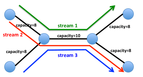
Consider the simple NUM problem described in Figure 1. Let $x_{1},x_{2}$ and $x_{3}$ be the data rates of stream $1,2$ and $3$ and let the network utility be minimizing $-\log(x_{1})-2\log(x_{2})-3\log(x_{3})$. It can be checked that capacity constraints other than $x_{1}+x_{2}+x_{3}\leq 10,x_{1}+x_{2}\leq 8,$ and $x_{2}+x_{3}\leq 8$ are redundant. By Theorem 11, the NUM problem can be formulated as follows:

$$\min\quad -\log(x_{1})-2\log(x_{2})-3\log(x_{3})$$

s.t. $$\mathbf{A}\mathbf{x}\leq\mathbf{b}$$

$$\mathbf{0}\leq\mathbf{x}\leq\mathbf{x}^{\max}$$

where $\mathbf{A}=\left[\begin{array}[]{ccc}1&1&1\\ 1&1&0\\ 0&1&1\end{array}\right]$, $\mathbf{b}=\left[\begin{array}[]{c}10\\ 8\\ 8\end{array}\right]$ and $\mathbf{x}^{\max}=\left[\begin{array}[]{c}11\\ 11\\ 11\end{array}\right]$. The optimal solution to this NUM problem is $x_{1}^{\ast}=2,x_{2}^{\ast}=3.2,x_{3}^{\ast}=4.8$ and the optimal value is $-7.7253$. Note that the second capacity constraint $x_{1}+x_{2}\leq 8$ is loose and the other two capacity constraints are tight.

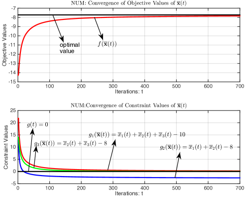
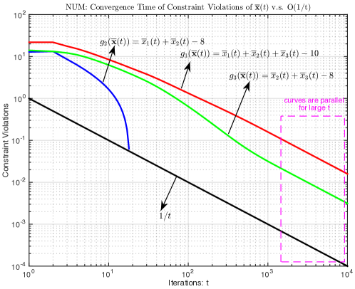
Since the objective function is decomposable, the dual subgradient method can yield a distributed solution. This is why the dual subgradient method is widely used to solve NUM problems [4]. It can be checked that the objective function is strongly convex with modulus $\alpha=\frac{2}{121}$ on $\mathcal{X}=\{\mathbf{0}\leq\mathbf{x}\leq\mathbf{x}^{\max}\}$ and $\mathbf{g}$ is Lipschitz continuous with modulus $\beta\leq\sqrt{6}$ on $\mathcal{X}$. Figure 2 verifies the convergence of $\overline{\mathbf{x}}(t)$ with $c=\frac{\alpha}{\beta^{2}}=1/363$ and $\lambda_{1}(0)=\lambda_{2}(0)=\lambda_{3}(0)=0$. Since $\lambda_{1}(0)=\lambda_{2}(0)=\lambda_{3}(0)=0$, by Theorem 1, we know $f(\overline{\mathbf{x}}(t))\leq f(\mathbf{x}^{\ast}),\forall t>0$, which is also verified in Figure 2. To verify the convergence time of constraint violations, Figure 3 plots $g_{1}(\overline{\mathbf{x}}(t))$, $g_{2}(\overline{\mathbf{x}}(t))$, $g_{3}(\overline{\mathbf{x}}(t))$ and $1/t$ with both x-axis and y-axis in $\log_{10}$ scales. As observed in Figure 3, the curves of $g_{1}(\overline{\mathbf{x}}(t))$ and $g_{3}(\overline{\mathbf{x}}(t))$ are parallel to the curve of $1/t$ for large $t$. Note that $g_{2}(\overline{\mathbf{x}}(t))\leq 0$ is satisfied early because this constraint is loose. Figure 3 verifies the convergence time of $\overline{\mathbf{x}}(t)$ in Theorem 3 by showing that error decays like $O(\frac{1}{t})$ and suggests that the convergence time is actually $\Theta(\frac{1}{\epsilon})$ for this NUM problem.

Figure 1: A simple NUM problem with $3$ flow streams

Figure 2: The convergence of $\overline{\mathbf{x}}(t)$ for a NUM problem.

Figure 3: The convergence time of $\overline{\mathbf{x}}(t)$ for a NUM problem.

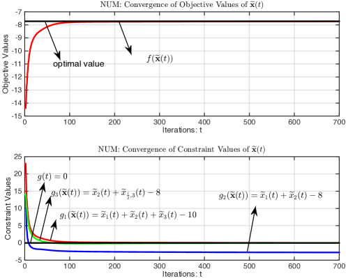
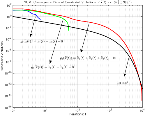
Note that $\text{rank}(\mathbf{A})=3$. By Theorem 11, this NUM problem satisfies Assumptions 1-4. Apply Algorithm 1 with $c=\frac{\alpha}{\beta^{2}}=1/363$ and $\lambda_{1}(0)=\lambda_{2}(0)=\lambda_{3}(0)=0$ to this NUM problem. Figure 4 verifies the convergence of the objective and constraint functions for $\widetilde{\mathbf{x}}(t)$. Figure 5 verifies the results in Theorem 11 that the convergence time of $\widetilde{\mathbf{x}}(t)$ is $O(\log(\frac{1}{\epsilon}))$ by showing that error decays like $O(\frac{1}{t}0.998^{t})$. If we compare Figure 5 and Figure 3, we can observe that $\widetilde{\mathbf{x}}(t)$ converges much faster than $\overline{\mathbf{x}}(t)$.

Figure 4: The convergence of $\widetilde{\mathbf{x}}(t)$ for a NUM problem.

Figure 5: The convergence time of $\widetilde{\mathbf{x}}(t)$ for a NUM problem.

VI-B Quadratic Programs (QPs) with Linear Constraints

Consider the following quadratic program (QP)

$$\min\quad \mathbf{x}^{T}\mathbf{P}\mathbf{x}+\mathbf{c}^{T}\mathbf{x}$$

s.t. $$\mathbf{A}\mathbf{x}\leq\mathbf{b}$$

where $\mathbf{P}=\left[\begin{array}[]{cc}1&2\\ 2&5\end{array}\right]$, $\mathbf{c}=[1,1]^{T}$, $\mathbf{A}=\left[\begin{array}[]{cc}1&1\\ 0&1\end{array}\right]$ and $\mathbf{b}=[-2,-1]^{T}$. The optimal solution to this quadratic program is $\mathbf{x}^{\ast}=\left[\begin{array}[]{c}-1\\ -1\end{array}\right]$ and the optimal value is $8$.

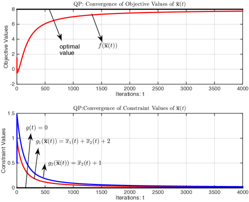
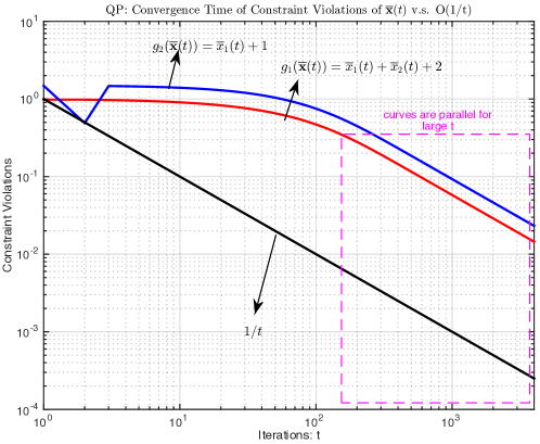
If $P$ is a diagonal matrix, the dual subgradient method can yield a distributed solution. It can be checked that the objective function is strongly convex with modulus $\alpha=0.34$ and each row of the linear inequality constraint is Lipschitz continuous with modulus $\zeta=\sqrt{2}$. Figure 6 verifies the convergence of $\overline{\mathbf{x}}(t)$ for the objective and constraint functions yielded by Algorithm 1 with $c=\frac{\alpha}{2\zeta^{2}}=0.34/4$, $\lambda_{1}(0)=0$ and $\lambda_{2}(0)=0$. Figure 7 verifies the convergence time of $\overline{\mathbf{x}}(t)$ proven in Theorem 3 by showing that error decays like $O(\frac{1}{t})$ and suggests that the convergence time is actually $\Theta(\frac{1}{\epsilon})$ for this quadratic program.

Figure 6: The convergence of $\overline{\mathbf{x}}(t)$ for a quadratic program.

Figure 7: The convergence time of $\overline{\mathbf{x}}(t)$ for a quadratic program.

Figure 8: The convergence of $\widetilde{\mathbf{x}}(t)$ for to a quadratic program.

Figure 9: The convergence time of $\widetilde{\mathbf{x}}(t)$ for a quadratic program.

Note that $\text{rank}(A)=2$. By Corollary 5 this quadratic program satisfies Assumptions 1-4.

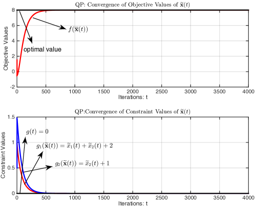
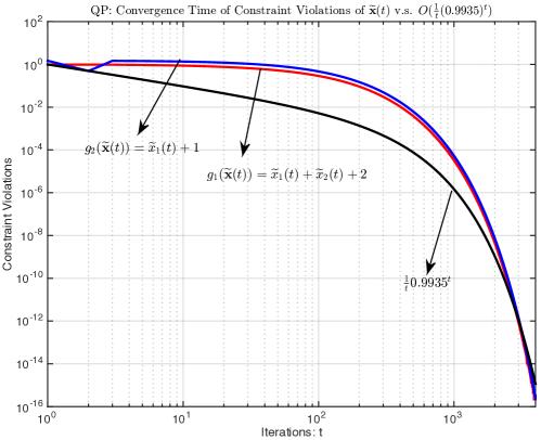
Apply Algorithm 1 with $c=\frac{\alpha}{2\zeta^{2}}=0.34/4$ and $\lambda_{1}(0)=\lambda_{2}(0)=\lambda_{3}(0)=0$ to this quadratic program. Figure 8 verifies the convergence of the objective and constraint functions. Figure 9 verifies the results in Corollary 5 that the convergence time of $\widetilde{\mathbf{x}}(t)$ is $O(\log(\frac{1}{\epsilon}))$ by showing that error decays like $O(\frac{1}{t}0.9935^{t})$. If we compare Figure 9 and Figure 7, we can observe that Algorithm $\widetilde{\mathbf{x}}(t)$ converges much faster than $\overline{\mathbf{x}}(t)$.

VI-C Large Scale Quadratic Programs

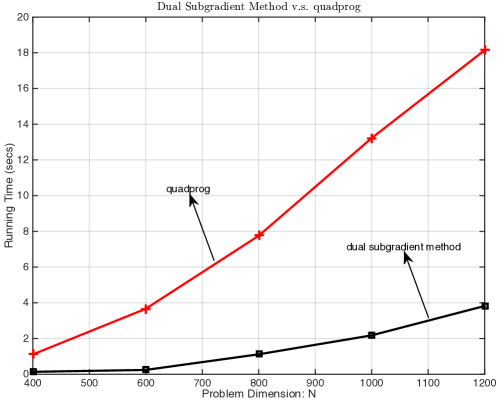
Consider quadratic program $\min_{\mathbf{x}\in\mathbb{R}^{N}}\{\mathbf{x}^{T}\mathbf{Q}\mathbf{x}+\mathbf{d}^{T}\mathbf{x}:\mathbf{A}\mathbf{x}\leq\mathbf{b}\}$ where $\mathbf{Q},\mathbf{A}\in\mathbb{R}^{N\times N}$ and $\mathbf{d},\mathbf{b}\in\mathbb{R}^{N}$. $\mathbf{Q}=\mathbf{U}\Sigma\mathbf{U}^{H}\in\mathbb{R}^{N\times N}$ where $\mathbf{U}$ is the orthonormal basis for a random $N\times N$ zero mean and unit variance normal matrix and $\Sigma$ is the diagonal matrix with entries from uniform $[1,3]$. $\mathbf{A}$ is a random $N\times N$ zero mean and unit variance normal matrix. $\mathbf{d}$ and $\mathbf{b}$ are random vectors with entries from uniform $[0,1]$. In a PC with a 4 core 2.7GHz Intel i7 Cpu and 16GB Memory, we run both Algorithm 1 and quadprog from Matlab, which by default is using the interior point method, over randomly generated large scale quadratic programs with $N=400,600,800,1000$ and $1200$. For different problem size $N$, the running time is the average over $100$ random quadratic programs and is plotted in Figure 10. To solve this large scale quadratic programs, the dual subgradient method has updates $\mathbf{x}(t)=-\frac{1}{2}\mathbf{Q}^{-1}[\boldsymbol{\lambda}^{T}(t)\mathbf{A}+\mathbf{d}]$ and $\boldsymbol{\lambda}(t+1)=\max\{\boldsymbol{\lambda}(t)+c[\mathbf{A}\mathbf{x}(t)-b],\mathbf{0}\}$ at each iteration $t$. Note that we only need to compute the inverse of large matrix $\mathbf{\mathbf{Q}}$ once and then use it during all iterations. In our numerical simulations, Algorithm 1 is terminated when the error (both objective violations and constraint violations) of $\widetilde{\mathbf{x}}(t)$ is less than 1e-5.

Figure 10: The average running time for large scale quadratic programs.

VII Conclusions

This paper studies the convergence time of the dual subgradient method strongly convex programs. This paper shows that the convergence time of the dual subgradient method with simple running averages for general strongly convex programs is $O(\frac{1}{\epsilon})$. This paper also considers a variation of the primal averages, called the sliding running averages, and shows that if the dual function is locally quadratic then the convergence time is $O(\log(\frac{1}{\epsilon}))$.

Appendix A Proof of Lemma 8

Note that $\lambda_{k}(t+1)=\max\{\lambda_{k}(t)+cg_{k}(\mathbf{x}(t)),0\},\forall k\in\{1,2,\ldots,m\}$ can be interpreted as the $\boldsymbol{\lambda}(t+1)=\mathcal{P}_{\mathbb{R}^{m}_{+}}\big{[}\boldsymbol{\lambda}(t)+c\mathbf{g}(\mathbf{x}(t))\big{]}$ where $\mathcal{P}_{\mathbb{R}^{m}_{+}}$ is the projection onto $\mathbb{R}^{m}_{+}$. As observed before, the dynamic of $\boldsymbol{\lambda}(t)$ can be interpreted as the projected gradient method with step size $c$ to solve $\max\limits_{\boldsymbol{\lambda}\in\mathbb{R}^{m}_{+}}\{q(\boldsymbol{\lambda})\}$. Thus, the proof given below is essentially the same as the convergence time proof of the projected gradient method for set constrained smooth optimization in [21].

Lemma 15 (Descent Lemma, Proposition A.24 in [7]).

Let $h$ be a continuously differentiable function. If $h$ is smooth on $\mathcal{X}$ with modulus $L$, then for any $\mathbf{x},\mathbf{y}\in\mathcal{X}$ we have

$$h(\mathbf{y}) \geq h(\mathbf{x})+\nabla h(\mathbf{x})^{T}(\mathbf{y}-\mathbf{x})-\frac{L}{2}||\mathbf{y}-\mathbf{x}||^{2},$$

$$h(\mathbf{y}) \leq h(\mathbf{x})+\nabla h(\mathbf{x})^{T}(\mathbf{y}-\mathbf{x})+\frac{L}{2}||\mathbf{y}-\mathbf{x}||^{2}.$$

Fact 1.

$\boldsymbol{\lambda}(t+1)=\operatorname*{argmax}_{\boldsymbol{\lambda}\in\mathbb{R}^{m}_{+}}\big{[}q(\boldsymbol{\lambda}(t))+[\mathbf{g}(\mathbf{x}(t))]^{T}[\boldsymbol{\lambda}-\boldsymbol{\lambda}(t)]-\frac{1}{2c}\|\boldsymbol{\lambda}-\boldsymbol{\lambda}(t)\|^{2}\big{]},\forall t\geq 0$.

Proof.

Fix $t\geq 0$,

$$\boldsymbol{\lambda}(t+1)= \mathcal{P}_{\mathbb{R}^{m}_{+}}\left[\boldsymbol{\lambda}(t)+c\mathbf{g}(\mathbf{x}(t))\right]$$

$$= \operatorname*{argmin}_{\boldsymbol{\lambda}\in\mathbb{R}^{m}_{+}}\|\boldsymbol{\lambda}-[\boldsymbol{\lambda}(t)+c\mathbf{g}(\mathbf{x}(t))]\|^{2}$$

$$= \operatorname*{argmin}_{\boldsymbol{\lambda}\in\mathbb{R}^{m}_{+}}\left[c^{2}\|\mathbf{g}(\mathbf{x}(t))\|^{2}-2c[\mathbf{g}(\mathbf{x}(t))]^{T}[\boldsymbol{\lambda}-\boldsymbol{\lambda}(t)]+\|\boldsymbol{\lambda}-\boldsymbol{\lambda}(t)\|^{2}\right]$$

$$\overset{(a)}{=} \operatorname*{argmin}_{\boldsymbol{\lambda}\in\mathbb{R}^{m}_{+}}\left[-q(\boldsymbol{\lambda}(t))-[\mathbf{g}(\mathbf{x}(t))]^{T}[\boldsymbol{\lambda}-\boldsymbol{\lambda}(t)]+\frac{1}{2c}\|\boldsymbol{\lambda}-\boldsymbol{\lambda}(t)\|^{2}\right]$$

$$= \operatorname*{argmax}_{\boldsymbol{\lambda}\in\mathbb{R}^{m}_{+}}\left[q(\boldsymbol{\lambda}(t))+[\mathbf{g}(\mathbf{x}(t))]^{T}[\boldsymbol{\lambda}-\boldsymbol{\lambda}(t)]-\frac{1}{2c}\|\boldsymbol{\lambda}-\boldsymbol{\lambda}(t)\|^{2}\right]$$

where (a) follows because the minimizer is unchanged when we remove constant term $c^{2}\|\mathbf{g}(\mathbf{x}(t))\|^{2}$, divide by factor $2c$, and add constant term $-q(\boldsymbol{\lambda}(t))$ in the objective function. ∎

Recall that $q(\boldsymbol{\lambda})$ is smooth with modulus $\gamma=\frac{\beta^{2}}{\alpha}$ by Lemma 7.

Fact 2.

If $c\leq\frac{1}{\gamma}=\frac{\alpha}{\beta^{2}}$, then $q(\boldsymbol{\lambda}(t+1))\geq q(\boldsymbol{\lambda}(t)),\forall t\geq 0$.

Proof.

Fix $t\geq 0$,

$$q(\boldsymbol{\lambda}(t+1))\overset{(a)}{\geq} q(\boldsymbol{\lambda}(t))+[\mathbf{g}(\mathbf{x}(t))]^{T}[\boldsymbol{\lambda}(t+1)-\boldsymbol{\lambda}(t)]-\frac{\gamma}{2}\|\boldsymbol{\lambda}(t+1)-\boldsymbol{\lambda}(t)\|^{2}$$

$$\overset{(b)}{\geq} q(\boldsymbol{\lambda}(t))+[\mathbf{g}(\mathbf{x}(t))]^{T}[\boldsymbol{\lambda}(t+1)-\boldsymbol{\lambda}(t)]-\frac{1}{2c}\|\boldsymbol{\lambda}(t+1)-\boldsymbol{\lambda}(t)\|^{2}$$

$$\overset{(c)}{\geq} q(\boldsymbol{\lambda}(t))+[\mathbf{g}(\mathbf{x}(t))]^{T}[\boldsymbol{\lambda}(t)-\boldsymbol{\lambda}(t)]-\frac{1}{2c}\|\boldsymbol{\lambda}(t)-\boldsymbol{\lambda}(t)\|^{2}$$

$$= q(\boldsymbol{\lambda}(t))$$

where (a) follows from Lemma 15 and the fact that $\nabla_{\boldsymbol{\lambda}}q(\boldsymbol{\lambda}(t))=\mathbf{g}(\mathbf{x}(t))$; (b) follows from $c\leq\frac{1}{\gamma}$; and (c) follows form Fact 1. ∎

Fact 3.

$\mathbf{g}^{T}(\mathbf{x}(t))[\boldsymbol{\lambda}(t+1)-\boldsymbol{\lambda}^{\ast}]\geq\frac{1}{c}[\boldsymbol{\lambda}(t+1)-\boldsymbol{\lambda}(t)]^{T}[\boldsymbol{\lambda}(t+1)-\boldsymbol{\lambda}^{\ast}],\forall t\geq 0$

Proof:

Fix $t\geq 0$. By the projection theorem (Proposition B.11(b) in [7]), we have $\big{[}\boldsymbol{\lambda}(t+1)-\big{(}\boldsymbol{\lambda}(t)+c\mathbf{g}(\mathbf{x}(t))\big{)}\big{]}^{T}[\boldsymbol{\lambda}(t+1)-\boldsymbol{\lambda}^{\ast}]\leq 0$. Thus, $\mathbf{g}^{T}(\mathbf{x}(t))[\boldsymbol{\lambda}(t+1)-\boldsymbol{\lambda}^{\ast}]\geq\frac{1}{c}[\boldsymbol{\lambda}(t+1)-\boldsymbol{\lambda}(t)]^{T}[\boldsymbol{\lambda}(t+1)-\boldsymbol{\lambda}^{\ast}]$. ∎

Fact 4.

If $c\leq\frac{1}{\gamma}=\frac{\alpha}{\beta^{2}}$, then $q(\boldsymbol{\lambda}^{\ast})-q(\boldsymbol{\lambda}(t+1))\leq\frac{1}{2c}\|\boldsymbol{\lambda}(t)-\boldsymbol{\lambda}^{\ast}\|^{2}-\frac{1}{2c}\|\boldsymbol{\lambda}(t+1)-\boldsymbol{\lambda}^{\ast}\|^{2},\forall t\geq 0$.

Proof:

Fix $t\geq 0$,

$$q(\boldsymbol{\lambda}(t+1))$$

$$\overset{(a)}{\geq} q(\boldsymbol{\lambda}(t))+[\mathbf{g}(\mathbf{x}(t))]^{T}[\boldsymbol{\lambda}(t+1)-\boldsymbol{\lambda}(t)]-\frac{\gamma}{2}\|\boldsymbol{\lambda}(t+1)-\boldsymbol{\lambda}(t)\|^{2}$$

$$= q(\boldsymbol{\lambda}(t))+[\mathbf{g}(\mathbf{x}(t))]^{T}[\boldsymbol{\lambda}(t+1)-\boldsymbol{\lambda}^{\ast}+\boldsymbol{\lambda}^{\ast}-\boldsymbol{\lambda}(t)]-\frac{\gamma}{2}\|\boldsymbol{\lambda}(t+1)-\boldsymbol{\lambda}(t)\|^{2}$$

$$\overset{(b)}{\geq} q(\boldsymbol{\lambda}(t))+[\mathbf{g}(\mathbf{x}(t))]^{T}[\boldsymbol{\lambda}^{\ast}-\boldsymbol{\lambda}(t)]-\frac{\gamma}{2}\|\boldsymbol{\lambda}(t+1)-\boldsymbol{\lambda}(t)\|^{2}+\frac{1}{c}[\boldsymbol{\lambda}(t+1)-\boldsymbol{\lambda}(t)]^{T}[\boldsymbol{\lambda}(t+1)-\boldsymbol{\lambda}^{\ast}]$$

$$\overset{(c)}{\geq} q(\boldsymbol{\lambda}(t))+[\mathbf{g}(\mathbf{x}(t))]^{T}[\boldsymbol{\lambda}^{\ast}-\boldsymbol{\lambda}(t)]-\frac{\gamma}{2}\|\boldsymbol{\lambda}(t+1)-\boldsymbol{\lambda}(t)\|^{2}+\frac{1}{2c}\|\boldsymbol{\lambda}(t+1)-\boldsymbol{\lambda}(t)\|^{2}+\frac{1}{2c}\|\boldsymbol{\lambda}(t+1)-\boldsymbol{\lambda}^{\ast}\|^{2}$$

$$-\frac{1}{2c}\|\boldsymbol{\lambda}(t)-\boldsymbol{\lambda}^{\ast}\|^{2}$$

$$\overset{(d)}{\geq} q(\boldsymbol{\lambda}(t))+[\mathbf{g}(\mathbf{x}(t))]^{T}[\boldsymbol{\lambda}^{\ast}-\boldsymbol{\lambda}(t)]+\frac{1}{2c}\|\boldsymbol{\lambda}(t+1)-\boldsymbol{\lambda}^{\ast}\|^{2}-\frac{1}{2c}\|\boldsymbol{\lambda}(t)-\boldsymbol{\lambda}^{\ast}\|^{2}$$

$$\overset{(e)}{\geq} q(\boldsymbol{\lambda}^{\ast})+\frac{1}{2c}\|\boldsymbol{\lambda}(t+1)-\boldsymbol{\lambda}^{\ast}\|^{2}-\frac{1}{2c}\|\boldsymbol{\lambda}(t)-\boldsymbol{\lambda}^{\ast}\|^{2}$$

where (a) follows from Lemma 15 and the fact that $\nabla_{\boldsymbol{\lambda}}q(\boldsymbol{\lambda}(t))=\mathbf{g}(\mathbf{x}(t))$; (b) follows from Fact 3; (c) follows from the identity $\mathbf{u}^{T}\mathbf{v}=\frac{1}{2}\|\mathbf{u}\|^{2}+\frac{1}{2}\|\mathbf{v}\|^{2}-\frac{1}{2}\|\mathbf{u}-\mathbf{v}\|^{2},\forall\mathbf{u},\mathbf{v}\in\mathbb{R}^{m}$; (d) follows from $c\leq\frac{1}{\gamma}$; and (e) follows from the concavity of $q(\cdot)$.

Rearranging terms yields the desired result. ∎

Fix $c\leq\frac{1}{\gamma}$ and $t>0$. By Fact 4, we have $q(\boldsymbol{\lambda}^{\ast})-q(\boldsymbol{\lambda}(\tau+1))\leq\frac{1}{2c}\|\boldsymbol{\lambda}(\tau)-\boldsymbol{\lambda}^{\ast}\|^{2}-\frac{1}{2c}\|\boldsymbol{\lambda}(\tau+1)-\boldsymbol{\lambda}^{\ast}\|^{2},\forall\tau\in\{0,1,\ldots,t-1\}$. Summing over $\tau$ and dividing by fact $t$ yields

$$\frac{1}{t}\sum_{\tau=0}^{t-1}\big{[}q(\boldsymbol{\lambda}^{\ast})-q(\boldsymbol{\lambda}(\tau+1))\big{]}\leq \frac{1}{2ct}[\|\boldsymbol{\lambda}(0)-\boldsymbol{\lambda}^{\ast}\|^{2}-\|\boldsymbol{\lambda}(t)-\boldsymbol{\lambda}^{\ast}\|^{2}]$$

$$\leq \frac{1}{2ct}\|\boldsymbol{\lambda}(0)-\boldsymbol{\lambda}^{\ast}\|^{2}$$

Note that $q(\boldsymbol{\lambda}^{\ast})-q(\boldsymbol{\lambda}(\tau+1)),\forall\tau\in\{0,1,\ldots,t-1\}$ is a decreasing sequence by Fact 2. Thus, we have

$$q(\boldsymbol{\lambda}^{\ast})-q(\boldsymbol{\lambda}(t)\leq\frac{1}{t}\sum_{\tau=0}^{t-1}\big{[}q(\boldsymbol{\lambda}^{\ast})-q(\boldsymbol{\lambda}(\tau+1))\big{]}\leq\frac{1}{2ct}\|\boldsymbol{\lambda}(0)-\boldsymbol{\lambda}^{\ast}\|^{2}.$$

Appendix B Proof of Part (2) of Lemma 11

This part is essentially a local version of Theorem 12 in [22], which shows that the projected gradient method for set constrained smooth convex optimization converge geometrically if the objective function satisfies a quadratic growth condition.

In this appendix, we provide a simple proof that directly follows from Fact 4 and Assumption 3. By Fact 4, we have

$$q(\boldsymbol{\lambda}^{\ast})-q(\boldsymbol{\lambda}(t+1))\leq\frac{1}{2c}\|\boldsymbol{\lambda}(t)-\boldsymbol{\lambda}^{\ast}\|^{2}-\frac{1}{2c}\|\boldsymbol{\lambda}(t+1)-\boldsymbol{\lambda}^{\ast}\|^{2},\forall t\geq 0.$$ (29)

By part (1), we know $\|\boldsymbol{\lambda}(t)-\boldsymbol{\lambda}^{\ast}\|\leq D_{q},\forall t\geq T_{q}$. By Assumption 3, we have

$$q(\boldsymbol{\lambda}^{\ast})-q(\boldsymbol{\lambda}(t+1))\geq L_{q}\|\boldsymbol{\lambda}(t+1)-\boldsymbol{\lambda}^{\ast}\|^{2},\forall t\geq T_{q}.$$ (30)

Combining (29) and (30) yields

$$(L_{q}+\frac{1}{2c})\|\boldsymbol{\lambda}(t+1)-\boldsymbol{\lambda}^{\ast}\|^{2}\leq\frac{1}{2c}\|\boldsymbol{\lambda}(t)-\boldsymbol{\lambda}^{\ast}\|^{2},\forall t\geq T_{q}.$$

This can be written as

$$\|\boldsymbol{\lambda}(t+1)-\boldsymbol{\lambda}^{\ast}\|\leq\sqrt{\frac{1}{1+2cL_{q}}}\|\boldsymbol{\lambda}(t)-\boldsymbol{\lambda}^{\ast}\|,\forall t\geq T_{q}.$$

By induction, we have

$$\|\boldsymbol{\lambda}(t)-\boldsymbol{\lambda}^{\ast}\|\leq\big{(}\sqrt{\frac{1}{1+2cL_{q}}}\big{)}^{t-T_{q}}\|\boldsymbol{\lambda}(T_{q})-\boldsymbol{\lambda}^{\ast}\|,\forall t\geq T_{q}.$$

Appendix C Proof of Lemma 13

Define $\tilde{h}(\mathbf{x})=-h(\mathbf{x})$. Then $\tilde{h}$ is smooth with modulus $\gamma$ and strongly convex with modulus $L_{c}$ over the set $\mathcal{X}$. By definition of smooth functions, $f$ must be differentiable over set $\mathcal{X}$. By Lemma 1, we have

$$\tilde{h}(\mathbf{y})\geq\tilde{h}(\mathbf{x})+[\nabla\tilde{h}(\mathbf{x})]^{T}(\mathbf{y}-\mathbf{x})+\frac{L_{c}}{2}\|\mathbf{y}-\mathbf{x}\|^{2},\forall\mathbf{x},\mathbf{y}\in\mathcal{X}$$

By Lemma 15,

$$\tilde{h}(\mathbf{y})\leq\tilde{h}(\mathbf{x})+[\nabla\tilde{h}(\mathbf{x})]^{T}(\mathbf{y}-\mathbf{x})+\frac{\gamma}{2}\|\mathbf{y}-\mathbf{x}\|^{2},\forall\mathbf{x},\mathbf{y}\in\mathcal{X}$$

Since $\mathcal{X}$ is not a singleton, we can choose distinct $\mathbf{x},\mathbf{y}\in\mathcal{X}$. Combining the above two inequalities yields $L_{c}\leq\gamma$.

Appendix D Proof of Part (2) of Lemma 14

By the first part of this lemma, $\boldsymbol{\lambda}(t)\in\{\boldsymbol{\lambda}\in\mathbb{R}^{m}_{+}:\|\boldsymbol{\lambda}-\boldsymbol{\lambda}^{\ast}\|\leq D_{c}\},\forall t\geq T_{c}$. The remaining part of the proof is essentially a local version of the convergence time proof of the projected gradient method for set constrained smooth and strongly convex optimization [21].

Recall that $q(\boldsymbol{\lambda})$ is smooth with modulus $\gamma=\frac{\beta^{2}}{\alpha}$ by Lemma 7. The next fact is an enhancement of Fact 4 using the locally strong concavity of the dual function.

Fact 5.

If $c\leq\frac{1}{\gamma}=\frac{\alpha}{\beta^{2}}$, then $q(\boldsymbol{\lambda}^{\ast})-q(\boldsymbol{\lambda}(t+1))\leq(\frac{1}{2c}-\frac{L_{c}}{2})\|\boldsymbol{\lambda}(t)-\boldsymbol{\lambda}^{\ast}\|^{2}-\frac{1}{2c}\|\boldsymbol{\lambda}(t+1)-\boldsymbol{\lambda}^{\ast}\|^{2},\forall t\geq T_{c}$.

Proof:

Fix $t\geq T_{c}$,

$$q(\boldsymbol{\lambda}(t+1))$$

$$\overset{(a)}{\geq} q(\boldsymbol{\lambda}(t))+[\mathbf{g}(\mathbf{x}(t))]^{T}[\boldsymbol{\lambda}(t+1)-\boldsymbol{\lambda}(t)]-\frac{\gamma}{2}\|\boldsymbol{\lambda}(t+1)-\boldsymbol{\lambda}(t)\|^{2}$$

$$= q(\boldsymbol{\lambda}(t))+[\mathbf{g}(\mathbf{x}(t))]^{T}[\boldsymbol{\lambda}(t+1)-\boldsymbol{\lambda}^{\ast}+\boldsymbol{\lambda}^{\ast}-\boldsymbol{\lambda}(t)]-\frac{\gamma}{2}\|\boldsymbol{\lambda}(t+1)-\boldsymbol{\lambda}(t)\|^{2}$$

$$\overset{(b)}{\geq} q(\boldsymbol{\lambda}(t))+[\mathbf{g}(\mathbf{x}(t))]^{T}[\boldsymbol{\lambda}^{\ast}-\boldsymbol{\lambda}(t)]-\frac{\gamma}{2}\|\boldsymbol{\lambda}(t+1)-\boldsymbol{\lambda}(t)\|^{2}+\frac{1}{c}[\boldsymbol{\lambda}(t+1)-\boldsymbol{\lambda}(t)]^{T}[\boldsymbol{\lambda}(t+1)-\boldsymbol{\lambda}^{\ast}]$$

$$\overset{(c)}{\geq} q(\boldsymbol{\lambda}(t))+[\mathbf{g}(\mathbf{x}(t))]^{T}[\boldsymbol{\lambda}^{\ast}-\boldsymbol{\lambda}(t)]-\frac{\gamma}{2}\|\boldsymbol{\lambda}(t+1)-\boldsymbol{\lambda}(t)\|^{2}+\frac{1}{2c}\|\boldsymbol{\lambda}(t+1)-\boldsymbol{\lambda}(t)\|^{2}+\frac{1}{2c}\|\boldsymbol{\lambda}(t+1)-\boldsymbol{\lambda}^{\ast}\|^{2}$$

$$-\frac{1}{2c}\|\boldsymbol{\lambda}(t)-\boldsymbol{\lambda}^{\ast}\|^{2}$$

$$\overset{(d)}{\geq} q(\boldsymbol{\lambda}(t))+[\mathbf{g}(\mathbf{x}(t))]^{T}[\boldsymbol{\lambda}^{\ast}-\boldsymbol{\lambda}(t)]+\frac{1}{2c}\|\boldsymbol{\lambda}(t+1)-\boldsymbol{\lambda}^{\ast}\|^{2}-\frac{1}{2c}\|\boldsymbol{\lambda}(t)-\boldsymbol{\lambda}^{\ast}\|^{2}$$

$$\overset{(e)}{\geq} q(\boldsymbol{\lambda}^{\ast})+\frac{1}{2c}\|\boldsymbol{\lambda}(t+1)-\boldsymbol{\lambda}^{\ast}\|^{2}+(\frac{L_{c}}{2}-\frac{1}{2c})\|\boldsymbol{\lambda}(t)-\boldsymbol{\lambda}^{\ast}\|^{2}$$

where (a) follows from Lemma 15 and the fact that $\nabla_{\boldsymbol{\lambda}}q(\boldsymbol{\lambda}(t))=\mathbf{g}(\mathbf{x}(t))$; (b) follows from Fact 3; (c) follows from the identity $\mathbf{u}^{T}\mathbf{v}=\frac{1}{2}\|\mathbf{u}\|^{2}+\frac{1}{2}\|\mathbf{v}\|^{2}-\frac{1}{2}\|\mathbf{u}-\mathbf{v}\|^{2},\forall\mathbf{u},\mathbf{v}\in\mathbb{R}^{m}$; (d) follows from $c\leq\frac{1}{\gamma}$; and (e) follows from the fact that $q(\cdot)$ is strongly concave over the set $\{\boldsymbol{\lambda}\in\mathbb{R}^{m}_{+}:\|\boldsymbol{\lambda}-\boldsymbol{\lambda}^{\ast}\|\leq D_{c}\}$ such that $q(\boldsymbol{\lambda}^{\ast})\leq q(\boldsymbol{\lambda}(t))+[\mathbf{g}(\mathbf{x}(t))]^{T}[\boldsymbol{\lambda}^{\ast}-\boldsymbol{\lambda}(t)]-\frac{L_{c}}{2}\|\boldsymbol{\lambda}^{\ast}-\boldsymbol{\lambda}(t)\|^{2}$ by Lemma 1.

Rearranging terms yields the desired inequality. ∎

Note that $q(\boldsymbol{\lambda}^{\ast})-q(\boldsymbol{\lambda}(t+1))\geq 0,\forall t>0$. Combining with Fact 5 yields $(\frac{1}{2c}-\frac{L_{c}}{2})\|\boldsymbol{\lambda}(t)-\boldsymbol{\lambda}^{\ast}\|^{2}-\frac{1}{2c}\|\boldsymbol{\lambda}(t+1)-\boldsymbol{\lambda}^{\ast}\|^{2}\geq 0,\forall t\geq T_{c}$. Recall that $c\leq\frac{1}{\gamma}$ implies that $c\leq\frac{1}{L_{c}}$ by Lemma 13. Thus, we have

$$\|\boldsymbol{\lambda}(t+1)-\boldsymbol{\lambda}^{\ast}\|\leq\sqrt{1-cL_{c}}\|\boldsymbol{\lambda}(t)-\boldsymbol{\lambda}^{\ast}\|,\forall t\geq T_{c}.$$

By induction, we have

$$\|\boldsymbol{\lambda}(t)-\boldsymbol{\lambda}^{\ast}\|\leq\big{(}\sqrt{1-cL_{c}}\big{)}^{t-T_{c}}\|\boldsymbol{\lambda}(T_{c})-\boldsymbol{\lambda}^{\ast}\|,\forall t\geq T_{c}.$$

Appendix E Proof of Theorem 10

Lemma 16.

Let $q(\boldsymbol{\lambda}):\mathbb{R}^{m}_{+}\rightarrow\mathbb{R}$ be a concave function and $q(\boldsymbol{\lambda})$ be maximized at $\boldsymbol{\lambda}=\boldsymbol{\lambda}^{\ast}\geq\mathbf{0}$. Denote $\mathbf{d}=\nabla_{\boldsymbol{\lambda}}q(\boldsymbol{\lambda}^{\ast})$ and $\mathbf{U}\boldsymbol{\Sigma}\mathbf{U}^{T}=\nabla_{\boldsymbol{\lambda}}^{2}q(\boldsymbol{\lambda}^{\ast})$. Suppose that the following conditions are satisfied:

1. Suppose $\mathbf{d}\leq\mathbf{0}$ and $\lambda_{k}^{\ast}d_{k}=0,\forall k\in\{1,\ldots,m\}$. Denote $\mathcal{K}=\{k\in\{1,\ldots,m\}:d_{k}=0\}$ and $l=|\mathcal{K}|$.

2. Suppose $\boldsymbol{\Sigma}\prec 0$ and $\text{rank}(\mathbf{U}^{\prime})=l$ where $\mathbf{U}^{\prime}$ is an $l\times n$ submatrix of $\mathbf{U}$ composed by rows with indices in $\mathcal{K}$.

Then, there exists $D_{q}>0$ and $L_{q}>0$ such that $q(\boldsymbol{\lambda})\leq q(\boldsymbol{\lambda}^{\ast})-L_{q}\|\boldsymbol{\lambda}-\boldsymbol{\lambda}^{\ast}\|^{2}$ for any $\boldsymbol{\lambda}\in\mathbb{R}^{m}_{+}$ and $\|\boldsymbol{\lambda}-\boldsymbol{\lambda}^{\ast}\|\leq D_{q}$.

Proof:

Without loss of generality, assume that $\mathcal{K}=\{1,\ldots,l\}$. Denote $\mathbf{U}=\left[\begin{array}[]{l}\mathbf{U}^{\prime}\\ \mathbf{U}^{\prime\prime}\end{array}\right]$ where $\mathbf{U}^{\prime\prime}$ is the $(m-l)\times n$ matrix composed by $(l+1)$-th to $m$-th rows of $\mathbf{U}$. Since $\mathbf{d}\leq\mathbf{0}$, we have $d_{i}<0$ for all $i\notin\mathcal{K}$ by definition of $\mathcal{K}$. Let $\delta=\min_{\{l+1\leq k\leq m\}}\{|d_{k}|\}$ such that $d_{k}\leq-\delta,\forall k\in\{l+1,\ldots,m\}$. For each $\boldsymbol{\lambda}$, we define $\boldsymbol{\mu}$ via $\mu_{k}=\lambda_{k}-\lambda_{k}^{\ast},\forall k\in\{1,\ldots,l\},\mu_{k}=0,\forall k\in\{l+1,\ldots,m\}$ and $\boldsymbol{\nu}$ via $\nu_{k}=0,\forall k\in\{1,\ldots,l\},\nu_{k}=\lambda_{k}-\lambda_{k}^{\ast},\forall k\in\{l+1,\ldots,m\}$ such that $\boldsymbol{\lambda}-\boldsymbol{\lambda}^{\ast}=\boldsymbol{\mu}+\boldsymbol{\nu}$ and $\|\boldsymbol{\lambda}-\boldsymbol{\lambda}^{\ast}\|^{2}=\|\boldsymbol{\mu}\|^{2}+\|\boldsymbol{\nu}\|^{2}$. Define $l$-dimension vector $\boldsymbol{\mu}^{\prime}=[\mu_{1},\ldots,\mu_{l}]$. Note that $\|\boldsymbol{\mu}^{\prime}\|=\|\boldsymbol{\mu}\|$. By the first condition, $d_{k}\neq 0,\forall k\in\{l+1,\ldots,m\}$ implies that $\lambda_{k}^{\ast}=0,\forall k\in\{l+1,\ldots,m\}$, which together with the fact that $\boldsymbol{\lambda}\geq\mathbf{0}$ implies that $\boldsymbol{\nu}\geq\mathbf{0}$. If $\|\boldsymbol{\lambda}-\boldsymbol{\lambda}^{\ast}\|$ is sufficiently small, we have

$$q(\boldsymbol{\lambda}) \overset{(a)}{=}q(\boldsymbol{\lambda}^{\ast})+(\boldsymbol{\lambda}-\boldsymbol{\lambda}^{\ast})^{T}\nabla_{\boldsymbol{\lambda}}q(\boldsymbol{\lambda}^{\ast})+(\boldsymbol{\lambda}-\boldsymbol{\lambda}^{\ast})^{T}\nabla^{2}_{\boldsymbol{\lambda}}q(\boldsymbol{\lambda}^{\ast})(\boldsymbol{\lambda}-\boldsymbol{\lambda}^{\ast})+o(\|\boldsymbol{\lambda}-\boldsymbol{\lambda}^{\ast}\|^{2})$$

$$=q(\boldsymbol{\lambda}^{\ast})+\sum_{k=1}^{l}\mu_{k}d_{k}+\sum_{k=l+1}^{m}\nu_{k}d_{k}+\boldsymbol{\mu}^{T}\mathbf{U}\boldsymbol{\Sigma}\mathbf{U}^{T}\boldsymbol{\mu}^{T}+\boldsymbol{\nu}^{T}\mathbf{U}\boldsymbol{\Sigma}\mathbf{U}^{T}\boldsymbol{\nu}^{T}+o(\|\boldsymbol{\lambda}-\boldsymbol{\lambda}^{\ast}\|^{2})$$

$$\overset{(b)}{\leq}q(\boldsymbol{\lambda}^{\ast})-\sum_{k=l+1}^{m}\nu_{k}\delta+\boldsymbol{\mu}^{\prime,T}\mathbf{U}^{\prime}\boldsymbol{\Sigma}\mathbf{U}^{\prime,T}\boldsymbol{\mu}^{\prime,T}+o(\|\boldsymbol{\lambda}-\boldsymbol{\lambda}^{\ast}\|^{2})$$

$$\overset{(c)}{\leq}q(\boldsymbol{\lambda}^{\ast})-\sum_{k=l+1}^{m}\nu_{k}\delta-\kappa\|\boldsymbol{\mu}^{\prime}\|^{2}+o(\|\boldsymbol{\lambda}-\boldsymbol{\lambda}^{\ast}\|^{2})$$

$$\overset{(d)}{<}q(\boldsymbol{\lambda}^{\ast})-\kappa\|\boldsymbol{\nu}\|^{2}-\kappa\|\boldsymbol{\mu}\|^{2}+o(\|\boldsymbol{\lambda}-\boldsymbol{\lambda}^{\ast}\|^{2})$$

$$=q(\boldsymbol{\lambda}^{\ast})-\kappa\|\boldsymbol{\lambda}-\boldsymbol{\lambda}^{\ast}\|^{2}+o(\|\boldsymbol{\lambda}-\boldsymbol{\lambda}^{\ast}\|^{2})$$

where (a) follows from the second-order Taylor’s expansion; (b) follows from the facts that $d_{k}=0,\forall k\in\{1,\ldots,l\}$; $\boldsymbol{\nu}\geq 0$ and $d_{k}\leq-\delta$; the last $m-l$ elements of vector $\boldsymbol{\mu}$ are zeros; and $\boldsymbol{\Sigma}\prec 0$; (c) is true because $\kappa>0$ exists when $\text{rank}(\mathbf{U}^{\prime})=l$ and $\boldsymbol{\Sigma}\prec 0$; and (d) follows from $-\delta\leq-\kappa\nu_{k},\forall k\in\{l+1,\ldots,m\}$, which is true as long as $\|\boldsymbol{\nu}\|$ is sufficiently small; and $\|\boldsymbol{\mu}^{\prime}\|=\|\boldsymbol{\mu}\|$.

By the definition of $o(\|\boldsymbol{\lambda}-\boldsymbol{\lambda}^{\ast}\|^{2})$, for any $\kappa>0$, we have $o(\|\boldsymbol{\lambda}-\boldsymbol{\lambda}^{\ast}\|^{2})\leq\frac{\kappa}{2}\|\boldsymbol{\lambda}-\boldsymbol{\lambda}^{\ast}\|^{2}$ as long as $\|\boldsymbol{\lambda}-\boldsymbol{\lambda}^{\ast}\|$ is sufficiently small. Thus, there exists $D_{q}>0$ such that

$$q(\boldsymbol{\lambda})\leq q(\boldsymbol{\lambda}^{\ast})-L_{q}\|\boldsymbol{\lambda}-\boldsymbol{\lambda}^{\ast}\|^{2},\forall\boldsymbol{\lambda}\in\{\boldsymbol{\lambda}\in\mathbb{R}^{m}_{+}:\|\boldsymbol{\lambda}-\boldsymbol{\lambda}^{\ast}\|\leq D_{q}\}$$

where $L_{s}=\kappa/2$. ∎

Lemma 17.

Let $q(\boldsymbol{\lambda}):\mathbb{R}^{m}_{+}\rightarrow\mathbb{R}$ be a second-order continuously differentiable concave function and $q(\boldsymbol{\lambda})$ be maximized at $\boldsymbol{\lambda}=\boldsymbol{\lambda}^{\ast}\geq\mathbf{0}$. If $\nabla_{\boldsymbol{\lambda}}^{2}q(\boldsymbol{\lambda}^{\ast})\prec 0$, then there exist $D_{c}>0$ and $L_{c}>0$ such that $q(\cdot)$ is strongly concave on the set $\boldsymbol{\lambda}\in\{\boldsymbol{\lambda}\in\mathbb{R}^{m}_{+}:\|\boldsymbol{\lambda}-\boldsymbol{\lambda}^{\ast}\|\leq D_{c}\}$

Proof:

This lemma trivially follows from the continuity of $\nabla_{\boldsymbol{\lambda}}^{2}q(\boldsymbol{\lambda})$. ∎

Proof of part (1) of Theorem 10:

Note that Assumption 1 is trivially true. Assumption 2 follows from the assumption that $\text{rank}(\nabla\mathbf{g}_{\mathcal{K}}(\mathbf{x}^{\ast})^{T})=l$. To show that Assumption 3 holds, we need to apply Lemma 16.

By the strong convexity of $f(\mathbf{x})$ and Proposition B.25 in [7], the dual function $q(\boldsymbol{\lambda})$ is differentiable and has gradient $\nabla_{\boldsymbol{\lambda}}q(\boldsymbol{\lambda}^{\ast})=\mathbf{g}(\mathbf{x}^{\ast})$. Thus, $\mathbf{d}=\nabla_{\boldsymbol{\lambda}}q(\boldsymbol{\lambda}^{\ast})\leq 0$. By Assumption 2, i.e., the strong duality, we have $\lambda_{k}^{\ast}d_{k}=0,\forall k\in\{1,\ldots,m\}$. Thus, the first condition in Lemma 16 is satisfied.

For $\boldsymbol{\lambda}\geq 0$, define $\mathbf{x}^{\ast}(\boldsymbol{\lambda})=\operatorname*{argmin}_{\mathbf{x}\in\mathbb{R}^{n}}\big{[}f(\mathbf{x})+\boldsymbol{\lambda}^{T}\mathbf{g}(\mathbf{x})\big{]}$ and note $\mathbf{x}^{\ast}=\mathbf{x}^{\ast}(\boldsymbol{\lambda}^{\ast})$. Note that $\mathbf{x}^{\ast}(\boldsymbol{\lambda})$ is a well-defined function because $f(\mathbf{x})+\boldsymbol{\lambda}^{T}\mathbf{g}(\mathbf{x})$ is strongly convex and hence is minimized at a unique point. By equation $(6.9)$, page 598, in [7], we have

$$\nabla^{2}_{\boldsymbol{\lambda}}q(\boldsymbol{\lambda}^{\ast})= -\Big{[}\nabla_{\mathbf{x}}\mathbf{g}(\mathbf{x}^{\ast})\Big{]}^{T}\Big{[}\nabla_{\mathbf{x}}^{2}f(\mathbf{x}^{\ast})+\sum_{k=1}^{m}\lambda_{k}^{\ast}\nabla_{\mathbf{x}}^{2}g_{k}(\mathbf{x}^{\ast})\Big{]}^{-1}\Big{[}\nabla_{\mathbf{x}}\mathbf{g}(\mathbf{x}^{\ast})\Big{]}$$ (31)

Note that $\nabla_{\mathbf{x}}^{2}f(\mathbf{x}^{\ast})+\sum_{k=1}^{m}\lambda_{k}^{\ast}\nabla_{\mathbf{x}}^{2}g_{k}(\mathbf{x}^{\ast})\succ 0$ because $f$ is strongly convex and $g_{k},k\in\{1,\ldots,m\}$ are convex. Thus, if $\text{rank}(\nabla_{\mathbf{x}}\mathbf{g}_{\mathcal{K}}(\mathbf{x}^{\ast})^{T})=|\mathcal{K}|$, then the second condition of Lemma 16 is satisfied.

Proof of part (2) of Theorem 10: Using the same argument, we can show that Assumptions 1-2 hold. By equation (31) and the assumption that $\text{rank}(\nabla_{\mathbf{x}}\mathbf{g}(\mathbf{x}^{\ast})^{T})=m$, Assumption 4 follows from Lemma 17.

Appendix F Proof of Theorem 11

• Proof of Part (1): Let $\mathbf{x}^{\ast}$ be the optimal solution to problem (21)-(23). Since each column of $\mathbf{A}$ has at least one non-zero entry, we have $x_{i}^{\ast}\leq b^{\max},\forall i\in\{1,2,\ldots,n\}$ with $b^{\max}=\max_{1\leq i\leq n}b_{i}$. Thus, problem (24)-(26) is equivalent to problem (21)-(23) since only a redundant constraint $\mathbf{x}\leq\mathbf{x}^{\max}$ is introduced.

• Proof of Part (2):

  • To show Assumption 1 holds: It follows from the strong convexity of $\sum_{i=1}^{n}-w_{i}\log(x_{i})$ over set $\mathcal{X}=\{\mathbf{0}\leq\mathbf{x}\leq\mathbf{x}^{\max}\}$.

  • To show Assumption 2 holds: It follows from the assumption that $\mathbf{A}\mathbf{x}^{\ast}\leq\mathbf{b}$, which is Slater’s condition for convex programs only with linear inequality constraints. (Or alternatively, Assumption 2 is also implied by the assumption that $\text{rank}(\mathbf{A}^{\prime})=m^{\prime}$, which is the linear independence constraint qualification for convex programs [6, 24].) Note that we can prove that Assumption 2 also holds for problem (21)-(23) with a similar argument.

  • To show Assumption 3 holds: Define the dual function of problem (21)-(23) as

    $$\tilde{q}(\boldsymbol{\lambda})=\min_{\mathbf{x}\geq\mathbf{0}}\Big{\{}\sum_{i=1}^{n}-w_{i}\log(x_{i})+\boldsymbol{\lambda}^{T}(\mathbf{A}\mathbf{x}-\mathbf{b})\Big{\}}.$$

    Since Assumption 2 holds for problem (21)-(23), we assume $(\mathbf{x}^{\ast},\boldsymbol{\lambda}^{\ast})$ be a primal-dual pair that attains the strong duality of problem (21)-(23). By the strong duality, $\mathbf{x}^{\ast}=\operatorname*{argmin}_{\mathbf{x}\geq\mathbf{0}}\big{[}\sum_{i=1}^{n}-w_{i}\log(x_{i})+(\boldsymbol{\lambda}^{\ast})^{T}(\mathbf{A}\mathbf{x}-\mathbf{b})\big{]}$, i.e, $x_{i}^{\ast}=\operatorname*{argmin}_{x_{i}\geq 0}\big{[}-w_{i}\log(x_{i})+(\boldsymbol{\lambda}^{\ast})^{T}\mathbf{a}_{i}x_{i}\big{]},\forall 1\leq i\leq n$. Thus, we have $x_{i}^{\ast}=\big{[}\frac{w_{i}}{(\boldsymbol{\lambda}^{\ast})^{T}\mathbf{a}_{i}}\big{]}_{0}^{\infty},\forall 1\leq i\leq n$. In the proof of part (1), we show that $0<x_{i}^{\ast}\leq b^{\max},\forall 1\leq i\leq n$. (Note that $x_{i}^{\ast}>0,\forall 1\leq i\leq n$ because the domain of $\log$ function is $(0,+\infty)$.) Thus, $0<\frac{w_{i}}{(\boldsymbol{\lambda}^{\ast})^{T}\mathbf{a}_{i}}\leq b^{\max}<x_{i}^{\max},\forall 1\leq i\leq n$ and $x_{i}^{\ast}=\big{[}\frac{w_{i}}{(\boldsymbol{\lambda}^{\ast})^{T}\mathbf{a}_{i}}\big{]}_{0}^{\infty}=\frac{w_{i}}{(\boldsymbol{\lambda}^{\ast})^{T}\mathbf{a}_{i}},\forall 1\leq i\leq n$.

    Now consider the equivalent problem (24)-(26), whose Lagrangian dual function is given by

    $$q(\boldsymbol{\lambda})=\min_{\mathbf{0}\leq\mathbf{x}\leq\mathbf{x}^{\max}}\big{\{}\sum_{i=1}^{n}-w_{i}\log(x_{i})+\boldsymbol{\lambda}^{T}(\mathbf{A}\mathbf{x}-\mathbf{b})\big{\}}.$$

    Note that $\mathbf{x}^{\ast}$ is still the optimal solution to problem (24)-(26). Note that $\operatorname*{argmin}_{\mathbf{0}\leq\mathbf{x}\leq\mathbf{x}^{\max}}\big{[}\sum_{i=1}^{n}-w_{i}\log(x_{i})+\boldsymbol{\lambda}^{T}(\mathbf{A}\mathbf{x}-\mathbf{b})\big{]}=\big{[}\big{[}\frac{w_{1}}{\boldsymbol{\lambda}^{T}\mathbf{a}_{1}}\big{]}_{0}^{x_{1}^{\max}},\ldots,\big{[}\frac{w_{n}}{\boldsymbol{\lambda}^{T}\mathbf{a}_{n}}\big{]}_{0}^{x_{n}^{\max}}\big{]}^{T}$. By the fact that $0<\frac{w_{i}}{(\boldsymbol{\lambda}^{\ast})^{T}\mathbf{a}_{i}}<x_{i}^{\max},\forall i\in\{1,2,\ldots,n\}$, we know $\big{[}\big{[}\frac{w_{1}}{(\boldsymbol{\lambda}^{\ast})^{T}\mathbf{a}_{1}}\big{]}_{0}^{x_{1}^{\max}},\ldots,\big{[}\frac{w_{n}}{(\boldsymbol{\lambda}^{\ast})^{T}\mathbf{a}_{n}}\big{]}_{0}^{x_{n}^{\max}}\big{]}^{T}=\big{[}\big{[}\frac{w_{1}}{(\boldsymbol{\lambda}^{\ast})^{T}\mathbf{a}_{1}}\big{]}_{0}^{\infty},\ldots,\big{[}\frac{w_{n}}{(\boldsymbol{\lambda}^{\ast})^{T}\mathbf{a}_{n}}\big{]}_{0}^{\infty}\big{]}^{T}$. Thus, $q(\boldsymbol{\lambda}^{\ast})=\tilde{q}(\boldsymbol{\lambda}^{\ast})$ and $\boldsymbol{\lambda}^{\ast}$ also attains the strong duality for the equivalent problem (24)-(26). By the continuity of functions $\frac{w_{i}}{\boldsymbol{\lambda}^{T}\mathbf{a}_{i}}$ and recall that $0<\frac{w_{i}}{(\boldsymbol{\lambda}^{\ast})^{T}\mathbf{a}_{i}}<x_{i}^{\max},\forall 1\leq i\leq n$ , we know $\big{[}\big{[}\frac{w_{1}}{\boldsymbol{\lambda}^{T}\mathbf{a}_{1}}\big{]}_{0}^{x_{1}^{\max}},\ldots,\big{[}\frac{w_{n}}{\boldsymbol{\lambda}^{T}\mathbf{a}_{n}}\big{]}_{0}^{x_{n}^{\max}}\big{]}^{T}=\big{[}\big{[}\frac{w_{1}}{\boldsymbol{\lambda}^{T}\mathbf{a}_{1}}\big{]}_{0}^{\infty},\ldots,\big{[}\frac{w_{n}}{\boldsymbol{\lambda}^{T}\mathbf{a}_{n}}\big{]}_{0}^{\infty}\big{]}^{T}=\big{[}\frac{w_{1}}{\boldsymbol{\lambda}^{T}\mathbf{a}_{1}},\ldots,\frac{w_{n}}{\boldsymbol{\lambda}^{T}\mathbf{a}_{n}}\big{]}^{T}$ when $\boldsymbol{\lambda}$ is sufficiently close to $\boldsymbol{\lambda}^{\ast}$.

    Next, we show that the dual function $q(\boldsymbol{\lambda})$ is locally quadratic in a neighborhood of $\boldsymbol{\lambda}^{\ast}$ by using Lemma 16. Consider $\boldsymbol{\lambda}\in\mathbb{R}^{m}_{+}$ such that $\|\boldsymbol{\lambda}-\boldsymbol{\lambda}^{\ast}\|$ is sufficiently small, or equivalently, $\boldsymbol{\lambda}$ is sufficiently close to $\boldsymbol{\lambda}^{\ast}$. For such $\boldsymbol{\lambda}$, we have

    $$\operatorname*{argmin}_{\mathbf{0}\leq\mathbf{x}\leq\mathbf{x}^{\max}}\big{[}\sum_{i=1}^{n}-w_{i}\log(x_{i})+\boldsymbol{\lambda}^{T}(\mathbf{A}\mathbf{x}-\mathbf{b})\big{]}=\big{[}\big{[}\frac{w_{1}}{\boldsymbol{\lambda}^{T}\mathbf{a}_{1}}\big{]}_{0}^{x_{1}^{\max}},\ldots,\big{[}\frac{w_{n}}{\boldsymbol{\lambda}^{T}\mathbf{a}_{n}}\big{]}_{0}^{x_{n}^{\max}}\big{]}^{T}=\big{[}\frac{w_{i}}{\boldsymbol{\lambda}^{T}\mathbf{a}_{1}},\ldots,\frac{w_{n}}{\boldsymbol{\lambda}^{T}\mathbf{a}_{n}}\big{]}^{T}$$

    Thus,

    $$q(\boldsymbol{\lambda}) =\sum_{i=1}^{n}\Big{[}-w_{i}\log\big{(}\frac{1}{\boldsymbol{\lambda}^{T}\mathbf{a}_{i}}\big{)}+\frac{w_{i}\boldsymbol{\lambda}^{T}\mathbf{a}_{i}}{\boldsymbol{\lambda}^{T}\mathbf{a}_{i}}\Big{]}-\boldsymbol{\lambda}^{T}\mathbf{b}$$

    $$=\sum_{i=1}^{n}\Big{[}-w_{i}\log\big{(}\frac{1}{\boldsymbol{\lambda}^{T}\mathbf{a}_{i}}\big{)}\Big{]}+\sum_{i=1}^{n}w_{i}-\boldsymbol{\lambda}^{T}\mathbf{b}$$

    for $\boldsymbol{\lambda}\in\mathbb{R}^{m}_{+}$ such that $\|\boldsymbol{\lambda}-\boldsymbol{\lambda}^{\ast}\|$ is sufficiently small. Note that $q(\boldsymbol{\lambda})$ given above is infinitely differentiable. Taking the first-order and second-order derivatives at $\boldsymbol{\lambda}=\boldsymbol{\lambda}^{\ast}$ yields

    $$\nabla_{\boldsymbol{\lambda}}q(\boldsymbol{\lambda}^{\ast}) =\sum_{i=1}^{n}\frac{w_{i}\mathbf{a}_{i}}{(\boldsymbol{\lambda}^{\ast})^{T}\mathbf{a}_{i}}-\mathbf{b},$$ (32)

    $$\nabla_{\boldsymbol{\lambda}}^{2}q(\boldsymbol{\lambda}^{\ast})= -\sum_{i=1}^{n}\frac{w_{i}\mathbf{a}_{i}\mathbf{a}_{i}^{T}}{((\boldsymbol{\lambda}^{\ast})^{T}\mathbf{a}_{i})^{2}}$$

    $$= \mathbf{A}\text{diag}\big{(}[-\frac{w_{1}}{((\boldsymbol{\lambda}^{\ast})^{T}\mathbf{a}_{i})^{2}},\ldots,-\frac{w_{n}}{((\boldsymbol{\lambda}^{\ast})^{T}\mathbf{a}_{n})^{2}}]\big{)}\mathbf{A}^{T},$$ (33)

    where $\text{diag}\big{(}[-\frac{w_{1}}{((\boldsymbol{\lambda}^{\ast})^{T}\mathbf{a}_{i})^{2}},\ldots,-\frac{w_{n}}{((\boldsymbol{\lambda}^{\ast})^{T}\mathbf{a}_{n})^{2}}]\big{)}$ denotes the diagonal matrix with diagonal entries given by

    $$-\frac{w_{1}}{((\boldsymbol{\lambda}^{\ast})^{T}\mathbf{a}_{i})^{2}},\ldots,-\frac{w_{n}}{((\boldsymbol{\lambda}^{\ast})^{T}\mathbf{a}_{n})^{2}}.$$

    Note that $\frac{w_{i}}{(\boldsymbol{\lambda}^{\ast})^{T}\mathbf{a}_{i}}>0,\forall 1\leq i\leq n$. Thus, if $\text{rank}(\mathbf{A}^{\prime})=m^{\prime}$, then Assumption 3 holds by Lemma 16.

• Proof of Part (3): Using the same arguments in the proof of part (2), we can show that Assumptions 1-2 hold. By equation (33) and the fact that $\text{rank}(\mathbf{A})=m$, Assumption 4 follows from Lemma 17.

References

- [1] H. Yu and M. J. Neely, “On the convergence time of the drift-plus-penalty algorithm for strongly convex programs,” in Proceedings of IEEE Conference on Decision and Control (CDC), 2015.
- [2] I. Necoara and V. Nedelcu, “Rate analysis of inexact dual first-order methods application to dual decomposition,” IEEE Transactions on Automatic Control, vol. 59, no. 5, pp. 1232–1243, May 2014.
- [3] H. Terelius, U. Topcu, and R. M. Murray, “Decentralized multi-agent optimization via dual decomposition,” in IFAC World Congress, 2011.
- [4] S. H. Low and D. E. Lapsley, “Optimization flow control—I: basic algorithm and convergence,” IEEE/ACM Transactions on Networking, vol. 7, no. 6, pp. 861–874, 1999.
- [5] S. H. Low, “A duality model of TCP and queue management algorithms,” IEEE/ACM Transactions on Networking, vol. 11, no. 4, pp. 525–536, 2003.
- [6] M. S. Bazaraa, H. D. Sherali, and C. M. Shetty, Nonlinear Programming: Theory and Algorithms. Wiley-Interscience, 2006.
- [7] D. P. Bertsekas, Nonlinear Programming, 2nd ed. Athena Scientific, 1999.
- [8] T. Larsson, M. Patriksson, and A.-B. Strömberg, “Ergodic, primal convergence in dual subgradient schemes for convex programming,” Mathematical programming, vol. 86, no. 2, pp. 283–312, 1999.
- [9] N. Z. Shor, Minimization Methods for Non-Differentiable Functions. Springer-Verlag, 1985.
- [10] H. D. Sherali and G. Choi, “Recovery of primal solutions when using subgradient optimization methods to solve lagrangian duals of linear programs,” Operations Research Letters, vol. 19, no. 3, pp. 105–113, 1996.
- [11] M. J. Neely, Stochastic Network Optimization with Application to Communication and Queueing Systems. Morgan & Claypool Publishers, 2010.
- [12] ——, “Distributed and secure computation of convex programs over a network of connected processors,” in DCDIS International Conference on Engineering Applications and Computational Algorithms, 2005.
- [13] ——, “A simple convergence time analysis of drift-plus-penalty for stochastic optimization and convex programs,” arXiv:1412.0791, 2014.
- [14] A. Nedić and A. Ozdaglar, “Approximate primal solutions and rate analysis for dual subgradient methods,” SIAM Journal on Optimization, vol. 19, no. 4, pp. 1757–1780, 2009.
- [15] S. Supittayapornpong, L. Huang, and M. J. Neely, “Time-average optimization with nonconvex decision set and its convergence,” in Proceedings of IEEE Conference on Decision and Control (CDC), 2014.
- [16] I. Necoara and A. Patrascu, “Iteration complexity analyisis of dual first order methods for conic convex programming,” Optimization Method and Software, vol. 31, no. 3, pp. 645–678, 2016.
- [17] I. Necoara, A. Patrascu, and A. Nedić, “Complexity certifications of first-order inexact lagrangian methods for general convex programming: Application to real-time mpc,” in Developments in Model-Based Optimization and Control. Springer, 2015, pp. 3–26.
- [18] M. J. Neely, “Dynamic power allocation and routing for satellite and wireless networks with time varying channels,” Ph.D. dissertation, Massachusetts Institute of Technology, 2003.
- [19] H. Yu and M. J. Neely, “A simple parallel algorithm with an convergence rate for general convex programs,” SIAM Journal on Optimization, vol. 27, no. 2, pp. 759–783, 2017.
- [20] J.-B. Hiriart-Urruty and C. Lemaréchal, Fundamentals of Convex Analysis. Springer, 2001.
- [21] Y. Nesterov, Introductory Lectures on Convex Optimization: A Basic Course. Springer Science & Business Media, 2004.
- [22] I. Necoara, Y. Nesterov, and F. Glineur, “Linear convergence of first order methods for non-strongly convex optimization,” arXiv:1504.06298v4, 2015.
- [23] F. P. Kelly, “Charging and rate control for elastic traffic,” European Transactions on Telecommunications, vol. 8, no. 1, pp. 33–37, 1997.
- [24] C. P. Simon and L. Blume, Mathematics for Economists. Norton New York, 1994.