Affine equivariant rank-weighted L-estimation of multivariate location

Abstract

In the multivariate one-sample location model, we propose a class of flexible robust, affine-equivariant L-estimators of location, for distributions invoking affine-invariance of Mahalanobis distances of individual observations. An involved iteration process for their computation is numerically illustrated.

1 Introduction

The affine-equivariance and its dual affine-invariance are natural generalizations of univariate translation-scale equivariance and invariance notions (Eaton 1983). Consider the group $\mathcal{C}$ of transformations of $\mathbb{R}_{p}$ to $\mathbb{R}_{p}$:

$$\mathbf{X}\mapsto\mathbf{Y}=\mathbf{B}\mathbf{X}+\mathbf{b},\;\mathbf{b}\in\mathbb{R}_{p}$$ (1)

where $\mathbf{B}$ is a positive definite $p\times p$ matrix. Generally with the choice of $\mathbf{B}$ we do not transform dependent coordinates of $\mathbf{X}$ to stochastically independent coordinates of $\mathbf{Y}.$ This is possible when $\mathbf{X}$ has a multi-normal distribution with mean vector $\theta$ and positive definite dispersion matrix $\mbox{\boldmath$\Sigma$},$ when letting $\mbox{\boldmath$\Sigma$}^{-1}=\mathbf{B}\mathbf{B}^{\top},$ so that $\mathbb{E}\mathbf{Y}=\mbox{\boldmath$\xi$}=\mathbf{B}\mbox{\boldmath$\theta$}+\mathbf{b}$ and dispersion matrix $\mathbf{B}\mbox{\boldmath$\Sigma$}\mathbf{B}^{\top}=\mathbf{I}_{p}.$ To construct and study the affine equivariant estimator of the location $\theta$ we need to consider some affine-invariant (AI) norm. The most well-known affine invariant norm is the Mahalanobis norm, whose squared version is

$$\mbox{\boldmath$\Delta$}^{2}=(\mathbf{X}-\mbox{\boldmath$\theta$})^{\top}\mbox{\boldmath$\Sigma$}^{-1}(\mathbf{X}-\mbox{\boldmath$\theta$})=\|\mathbf{X}-\mbox{\boldmath$\theta$}\|^{2}_{\Sigma}$$ (2)

where $\Sigma$ is the dispersion matrix of $\mathbf{X}.$ To incorporate this norm, we need to use its empirical version based on independent sample $\mathbf{X}_{1},\ldots,\mathbf{X}_{n},$ namely

$$s_{ij}=\frac{1}{2}(\mathbf{X}_{i}-\mathbf{X}_{j})^{\top}\mathbf{V}_{n}^{*-1}(\mathbf{X}_{i}-\mathbf{X}_{j}),\;1\leq i<j\leq n$$

where $\mathbf{V}_{n}^{*}=(n(n-1))^{-1}\sum_{1\leq i<j\leq n}(\mathbf{X}_{i}-\mathbf{X}_{j})(\mathbf{X}_{i}-\mathbf{X}_{j})^{\top}.$ To avoid redundancy, we may consider the reduced set

$$\tilde{d}_{ni}=(\mathbf{X}_{i}-\mathbf{X}_{n})^{\top}\tilde{\mathbf{V}}_{n}^{-1}(\mathbf{X}_{i}-\mathbf{X}_{n}),\;i=1,\ldots,n-1$$ (3)

$$\tilde{\mathbf{V}}_{n}=\sum_{i=1}^{n-1}(\mathbf{X}_{i}-\mathbf{X}_{n})(\mathbf{X}_{i}-\mathbf{X}_{n})^{\top}$$ (4)

which forms the maximal invariant (MI) with respect to affine transformations (1). An equivalent form of the maximal invariant is

$${d}_{ni}=(\mathbf{X}_{i}-\overline{\mathbf{X}}_{n})^{\top}{\mathbf{V}}_{n}^{-1}(\mathbf{X}_{i}-\overline{\mathbf{X}}_{n}),\;i=1,\ldots,n$$ (5)

$${\mathbf{V}}_{n}=\sum_{i=1}^{n}(\mathbf{X}_{i}-\overline{\mathbf{X}}_{n})(\mathbf{X}_{i}-\overline{\mathbf{X}}_{n})^{\top}$$ (6)

(Obenchain (1971)). Note that all the $d_{ni}$ are between 0 and 1 and their sum equals to $p.$ Because $d_{ni}$ are exchangeable, bounded random variables, all nonnegative, with a constant sum equal to $p,$ the asymptotic properties of the array $(d_{n1},\ldots,d_{nn})^{\top}$ follow from Chernoff and Teicher (1958) and Weber (1980). Similarly, $\sum_{i=1}^{n-1}\tilde{d}_{ni}=p.$ Neither $\overline{\mathbf{X}}_{n}$ nor $\mathbf{V}_{n}$ is robust against outliers and gross errors contamination. As such, we are motivated to replace $\overline{X}_{n}$ and $\mathbf{V}_{n}$ by suitable robust versions and incorporate them in the formulation of a robust affine equivariant estimator of $\mbox{\boldmath$\theta$}.$ If $\widehat{\mbox{\boldmath$\theta$}}_{n}$ is some affine equivariant estimator of $\mbox{\boldmath$\theta$},$ then writing

$$\widehat{\mathbf{V}}_{n}=\sum_{i=1}^{n}(\mathbf{X}_{i}-\widehat{\mbox{\boldmath$\theta$}}_{n})(\mathbf{X}_{i}-\widehat{\mbox{\boldmath$\theta$}}_{n})^{\top}$$

we may note that $\widehat{\mathbf{V}}_{n}$ is smaller than $\mathbf{V}_{n}$ in the matrix sense. However, it cannot be claimed that the Mahalanobis distances (5) can be made shorter by using $\widehat{\mbox{\boldmath$\theta$}}_{n}$ instead of $\overline{\mathbf{X}}_{n},$ because $\sum_{i=1}^{n}(\mathbf{X}_{i}-\widehat{\mbox{\boldmath$\theta$}}_{n})^{\top}\widehat{\mathbf{V}}_{n}^{-1}(\mathbf{X}_{i}-\widehat{\mbox{\boldmath$\theta$}}_{n})=p.$ Our motivation is to employ the robust Mahalanobis distances in the formulation of robust affine equivariant estimator of $\mbox{\boldmath$\theta$},$ through a tricky ranking of the Mahalanobis distances in (5) and an iterative procedure in updating an affine equivariant robust estimator of $\mbox{\boldmath$\theta$}.$

The robust estimators in the multivariate case, discussed in detail in Jurečková et al. (2013), are not automatically affine equivariant. With due emphasize on the spatial median, some other estimators were considered by a host of researchers, and we refer to Oja (2010) and Serfling (2010) for a detailed account. Their emphasis is on the spatial median and spatial quantile functions defined as follows:
Let $\mathcal{B}_{p-1}(\mathbf{0})$ be the open unit ball. Then the $\mathbf{u}$-th spatial quantile $Q_{F}(\mathbf{u}),\;\mathbf{u}\in\mathcal{B}_{p-1}(\mathbf{0})$ is defined as the solution ${\mathbf{x}}=Q_{F}(\mathbf{u})$ of the equation

$$\mathbf{u}=\mathbb{E}\left\{\frac{{\mathbf{x}}-\mathbf{X}}{\|{\mathbf{x}}-\mathbf{X}\|}\right\},\quad\mathbf{u}\in\mathcal{B}_{p-1}(\mathbf{0}).$$

Particularly, $Q_{F}(\mathbf{0})$ is the spatial median. It is equivariant with respect to $\mathbf{y}=\mathbf{B}\mathbf{x}+\mathbf{b},\;\mathbf{b}\in\mathbb{R}_{p},\;\mathbf{B}$ positive definite and orthogonal. However, the spatial quantile function may not be affine-equivariant for all $\mathbf{u}.$

Among various approaches to multivariate quantiles we refer to Chakraborty (2001), Roelant and van Aelst (2007), Hallin et al. (2010), Kong and Mizera (2012), Jurečková et al. (2013), among others. Lopuha$\ddot{\rm a}$ & Rousseeuw (1991) and Zuo (2003, 2004 2006), Lopuha$\ddot{\rm a}$ & Rousseeuw (1991) and Zuo (2003, 2004 2006), among others, studied robust affine-equivariant estimators with high breakdown point, based on projection debths. An alternative approach based on the notion of the depth function and associated U-statistics has been initiated by Liu at al. (1999). Notice that every affine-invariant function of $(\mathbf{X}_{1},\ldots,\mathbf{X}_{n})$ depends on the $\mathbf{X}_{i}$ only through the maximal invariant; particularly, this applies to the ranks of the $d_{ni}$ and also to all affine invariant depths considered in the literature. In our formulation, affine equivariance property is highlighted and accomplished through a ranking of the Mahalanobis distances at various steps.

2 Affine equivariant linear estimators

Let $\mathbf{X}\in\mathbb{R}_{p}$ be a random vector with a distribution function $F.$ Unless stated otherwise, we assume that $F$ is absolutely continuous. Consider the qroup $\mathcal{C}$ of affine transformations $\mathbf{X}\mapsto\mathbf{Y}=\mathbf{B}\mathbf{X}+\mathbf{b}$ with $\mathbf{B}$ nonsingular of order $p\times p,$ $\mathbf{b}\in\mathbb{R}_{p}.$ Each transformation generates a distribution function $G$ also defined on $\mathbb{R}_{p},$ which we denote $G=F_{B,b}.$ A vector-valued functional $\mbox{\boldmath$\theta$}(F),$ designated as a suitable measure of location of $F,$ is said to be an affine-equivariant location functional, provided

$$\mbox{\boldmath$\theta$}(F_{B,b})=\mathbf{B}\mbox{\boldmath$\theta$}(F)+\mathbf{b}\quad\forall\mathbf{b}\in\mathbb{R}_{p},\;\mathbf{B}\;\mbox{ positive definite}.$$

Let $\mbox{\boldmath$\Gamma$}(F)$ be a matrix valued functional of $F,$ designated as a measure of the scatter of $F$ around its location $\theta$ and capturing its shape in terms of variation and covariation of the coordinate variables. $\mbox{\boldmath$\Gamma$}(F)$ is often termed a covariance functional, and a natural requirement is that it is independent of $\mbox{\boldmath$\theta$}(F).$ It is termed an affine-equivariant covariance functional, provided

$$\mbox{\boldmath$\Gamma$}(F_{B,b})=\mathbf{B}\mbox{\boldmath$\Gamma$}(F)\mathbf{B}^{\top}\quad\forall\mathbf{b}\in\mathbb{R}_{p},\;\mathbf{B}\;\mbox{ positive definite}.$$

We shall construct a class of affine equivariant L-estimators of location parameter, starting with initial affine-equivariant location estimator and scale functional, and then iterating them to a higher robustness. For simplicity we start with the sample mean vector $\overline{\mathbf{X}}_{n}=\frac{1}{n}\sum_{i=1}^{n}\mathbf{X}_{i}$ and with the matrix $\mbox{\boldmath$V$}_{n}=\mathbf{A}_{n}^{(0)}=\sum_{i=1}^{n}(\mathbf{X}_{i}-\overline{\mathbf{X}}_{n})(\mathbf{X}_{i}-\overline{\mathbf{X}}_{n})^{\top}=n\widehat{\mbox{\boldmath$\Sigma$}}_{n},\;n>p,$ where $\widehat{\mbox{\boldmath$\Sigma$}}_{n}$ is the sample covariance matrix. Let $R_{ni}=\sum_{j=1}^{n}I[d_{nj}\leq d_{ni}]$ be the rank of $d_{ni}$ among $d_{n1},\ldots,d_{nn},\;i=1,\ldots,n,$ and denote $\mathbf{R}_{n}=(R_{n1},\ldots,R_{nn})^{\top}$ the vector of ranks. Because $F$ is continuous, the probability of ties is 0, hence the ranks are well defined. Note that $d_{ni}$ and $R_{ni}$ are affine-invariant, $i=1,\ldots,n.$ Moreover, the $R_{ni}$ are invariant under any strictly monotone transformation of $d_{ni},\;i=1,\ldots,n.$ Furthermore, each $\mathbf{X}_{i}$ is trivially affine-equivariant. We introduce the following (Mahalanobis) ordering of $\mathbf{X}_{1},\ldots,\mathbf{X}_{n}:$

$$\mathbf{X}_{i}\prec\mathbf{X}_{j}\;\Leftrightarrow\;d_{ni}<d_{nj},\;i\neq j=1,\ldots,n.$$ (7)

This affine invariant ordering leads to vector of order statistics $\mathbf{X}_{n:1}\prec\ldots\prec\mathbf{X}_{n:n}$ of the sample $\mathbb{X}_{n}$. In the univariate case with the order statistics $X_{n:1}\leq\ldots\leq X_{n:n}$, we can consider the $k$-order rank weighted mean (Sen (1964)) defined as

$$T_{nk}=\left(\begin{array}[]{c}n\\ 2k+1\\ \end{array}\right)^{-1}\sum_{i=k+1}^{n-k}\left(\begin{array}[]{c}i-1\\ k\\ \end{array}\right)\left(\begin{array}[]{c}n-1\\ k\\ \end{array}\right)X_{n:i},\quad k=0,\ldots,\left[\frac{n+1}{2}\right].$$

For $k=0,\;T_{nk}=\overline{X}_{n}$ and $k=[(n+1)/2]$ leads to the median $\widetilde{X}_{n}.$ In the multivariate case, the ordering is induced by the non-negative $d_{ni}$, and the smallest $d_{ni}$ corresponds to the smallest outlyingness from the center, or to the nearest neighborhood of the center. Keeping that in mind, we can conceive by a sequence $\{k_{n}\}$ of nonnegative integers, such that $k_{n}$ is $\nearrow$ in $n,$ but $n^{-1/2}k_{n}$ is $\searrow$ in $n,$ and for fixed $k$ put

$$\mathbf{L}_{nk}=\left(\begin{array}[]{c}k_{n}\\ k\\ \end{array}\right)^{-1}\sum_{i=1}^{n}I\left[R_{ni}\leq k_{n}\right]\left(\begin{array}[]{c}k_{n}-R_{ni}\\ k-1\\ \end{array}\right)\mathbf{X}_{i}.$$

$\mathbf{L}_{nk}$ is affine-equivariant, because the $d_{ni}$ are affine invariant and the $\mathbf{X}_{i}$ are trivially affine equivariant. Of particular interest is the case of $k=1,$ i.e.,

$$\mathbf{L}_{n1}=k_{n}^{-1}\sum_{i=1}^{n}I\left[R_{ni}\leq k_{n}\right]\mathbf{X}_{i}$$

representing a trimmed, rank-weighted, nearest neighbor (NN) affine-equivariant estimator of $\mbox{\boldmath$\theta$}.$ In the case $k=2$ we have

$$\mathbf{L}_{n2}=\left(\begin{array}[]{c}k_{n}\\ 2\\ \end{array}\right)^{-1}\sum_{i=1}^{n}I\left[R_{ni}\leq k_{n}\right](k_{n}-R_{ni})\mathbf{X}_{i}$$

which can be rewritten as $\quad\mathbf{L}_{n2}=\sum_{i=1}^{n}w_{nR_{ni}}\mathbf{X}_{i}$ with the weight-function

$$w_{ni}=\left\{\begin{array}[]{lll}\left(\begin{array}[]{c}k_{n}\\ 2\\ \end{array}\right)^{-1}(k_{n}-i)&\ldots&i=1,\ldots,k_{n};\\[8.53581pt] \quad 0&\ldots&i>k_{n}.\\ \end{array}\right.$$

We see that $\mathbf{L}_{n}$ puts greater influence for $R_{ni}=1$ or 2, and $w_{nk_{n}}=0;\;w_{n1}=2/k_{n}.$ For $k\geq 3,$ even greater weights will be given to $R_{ni}=1$ or 2, etc. For large $n$ we can use the Poisson weights, following Chaubey and Sen (1996):

$$w^{0}_{ni}=\left(1-\rm e^{-\lambda}\right)^{-1}\frac{\rm e^{-\lambda}\lambda^{i}}{i!},\;\lambda<1,\;i=1,2,\ldots.$$

A typical $\lambda$ is chosen somewhere in the middle of $[0,1].$ Then $\mathbf{L}_{n}^{0}=\sum_{i=1}^{n}w_{nR_{ni}}^{0}\mathbf{X}_{i}$ represents an untrimmed smooth affine-equivariant L-estimator of $\mbox{\boldmath$\theta$};$ for $\lambda\rightarrow 0$ we get the median affine-equivariant estimator, while $\lambda\rightarrow 1$ gives a version of $L_{n2}$-type estimator. If $\lambda$ is chosen close to 1/2 and $k_{n}=o(\sqrt{n}),$ then tail $\sum_{j>k_{n}}w_{nj}^{(0)}$ converges exponentially to 0, implying a fast negligibility of the tail. Parallelly, the weights $w_{n}(i)$ can be chosen as the nonincreasing rank scores $a_{n}(1)\geq a_{n}(2)\geq\ldots\geq a_{n}(n).$

To diminish the influence of the initial estimators, we can recursively continue in the same way: Put $\mathbf{L}_{n}^{(1)}=\mathbf{L}_{n}$ and define in the next step:

$$\mathbf{A}_{n}^{(1)}=\sum_{i=1}^{n}(\mathbf{X}_{i}-\mathbf{L}_{n}^{(1)})(\mathbf{X}_{i}-\mathbf{L}_{n}^{(1)})^{\top}$$

$$d_{ni}^{(1)}=(\mathbf{X}_{i}-\mathbf{L}_{n}^{(1)})^{\top}(\mathbf{A}_{n}^{(1)})^{-1}(\mathbf{X}_{i}-\mathbf{L}_{n}^{(1)})$$

$$R_{ni}^{(1)}=\sum_{j=1}^{n}I[d_{nj}^{(1)}\leq d_{ni}^{(1)}],\;i=1,\ldots,n,\quad\mathbf{R}_{n}^{(1)}=(R_{n1}^{(1)},\ldots,R_{nn}^{(1)})^{\top}.$$

The second-step estimator is $\mathbf{L}_{n}^{(2)}=\sum_{i=1}^{n}w_{n}(R_{ni}^{(1)})\mathbf{X}_{i}.$ In this way we proceed, so at the $r$-th step we define $\mathbf{A}_{n}^{(r)},\;d_{ni}^{(r)},\;1\leq i\leq n$ and the ranks $\mathbf{R}_{n}^{(r)}$ analogously, and get the $r$-step estimator

$$\mathbf{L}_{n}^{(r)}=\sum_{i=1}^{n}w_{n}(R_{ni}^{(r-1)})\mathbf{X}_{i},\;r\geq 1.$$ (8)

Note that the $d_{ni}^{(r)}$ are affine-invariant for every $1\leq i\leq n$ and for every $r\geq 0.$ Hence, applying an affine transformation $\mathbf{Y}_{i}=\mathbf{B}\mathbf{X}_{i}+\mathbf{b},\;\mathbf{b}\in\mathbb{R}_{p},\;\mathbf{B}$ positive definite, we see that

$$\mathbf{L}_{n}^{(r)}(\mathbf{Y}_{1},\ldots,\mathbf{Y}_{n})=\mathbf{B}\mathbf{L}_{n}^{(r)}(\mathbf{X}_{1},\ldots,\mathbf{X}_{n})+\mathbf{b}.$$ (9)

Hence, the estimating procedure preserves the affine equivariance at each step and $\mathbf{L}_{n}^{(r)}$ is an affine-equivariant L-estimator of $\theta$ for every $r.$

The algorithm proceeds as follows:

•

(1)  Calculate $\overline{\mathbf{X}}_{n}$ and $\mathbf{A}_{n}^{(0)}=\sum_{i=1}^{n}(\mathbf{X}_{i}-\overline{\mathbf{X}}_{n})(\mathbf{X}_{i}-\overline{\mathbf{X}}_{n})^{\top}.$

•

(2)  Calculate $d_{ni}^{(0)}=(\mathbf{X}_{i}-\overline{\mathbf{X}}_{n})^{\top}(\mathbf{A}_{n}^{(0)})^{-1}(\mathbf{X}_{i}-\overline{\mathbf{X}}_{n}),\;1\leq i\leq n.$

•

(3)  Determine the rank $R_{ni}^{(0)}$ of $d_{ni}^{(0)}$ among $d_{n1}^{(0)},\ldots,d_{nn}^{(0)},\;i=1,\ldots,n.$

•

(4)  Calculate the scores $a_{n}(i),\;i=1,\ldots,n$

•

(5)  Calculate the first-step estimator $\mathbf{L}_{n}^{(1)}=\sum_{i=1}^{n}a_{n}(R_{ni}^{(0)})\mathbf{X}_{i}.$

•

(6)  $\mathbf{A}_{n}^{(1)}=\sum_{i=1}^{n}(\mathbf{X}_{i}-\mathbf{L}_{n}^{(1)})(\mathbf{X}_{i}-\mathbf{L}_{n}^{(1)})^{\top}.$

•

(7)  $d_{ni}^{(1)}=(\mathbf{X}_{i}-\mathbf{L}_{n}^{(1)})^{\top}(\mathbf{A}_{n}^{(1)})^{-1}(\mathbf{X}_{i}-\mathbf{L}_{n}^{(1)}),\;1\leq i\leq n.$

•

(8)  $R_{ni}^{(1)}=$ the rank of $d_{ni}^{(1)}$ among $d_{n1}^{(1)},\ldots,d_{nn}^{(1)},\;i=1,\ldots,n.$

•

(9)  $\mathbf{L}_{n}^{(2)}=\sum_{i=1}^{n}a_{n}(R_{ni}^{(1)})\mathbf{X}_{i}.$

•

(10) Repeat the steps (6)–(9).

The estimator $\mathbf{L}_{n}^{(r)}$ is a linear combination of order statistics corresponding to independent random vectors $\mathbf{X}_{1},\ldots,\mathbf{X}_{n},$ with random coefficients based on the exchangeable $d_{ni}^{(r)}.$ The asymptotic distribution of $\mathbf{L}_{n}^{(r)}$ under fixed $r$ and for $n\rightarrow\infty$ is a problem for a future study, along with the asymptotic distribution of the $d_{ni}^{(r)}$ and of the rank statistics. For the moment, let us briefly recapitulate some asymptotic properties of the $d_{ni}^{(r)}.$ Note that $\sum_{i=1}^{n}d_{ni}^{(r)}=p\quad\forall~{}r\geq 0,$ and that the $d_{ni}^{(r)}$ are exchangeable nonnegative random variables with a constant sum and $\mathbb{E}(d_{ni}^{(r)})=\frac{p}{n}$ for every $r\geq 0.$ Let $\delta_{ni}^{(r)}=(\mathbf{X}_{i}-\mathbf{L}_{n}^{(r)})^{\top}\mbox{\boldmath$\Sigma$}^{-1}(\mathbf{X}_{i}-\mathbf{L}_{n}^{(r)})$ and $\delta_{i}^{*}=(\mathbf{X}_{i}-\mbox{\boldmath$\theta$})^{\top}\mbox{\boldmath$\Sigma$}^{-1}(\mathbf{X}_{i}-\mbox{\boldmath$\theta$}),\;1\leq i\leq n,\;r\geq 1$ where $\Sigma$ is the covariance matrix of $\mathbf{X}_{1}.$ Let $G_{n}^{(r)}(y)=P\{nd_{ni}^{(r)}\leq y\}$ be the distribution function of the ${n}d_{ni}^{(r)}$ and let $\widehat{G}_{n}^{(r)}(y)=n^{-1}\sum_{i=1}^{n}I[nd_{ni}^{(r)}\leq y],\;y\in\mathbb{R}^{+}$ be the empirical distribution function. Side by side, let $G_{nr}^{*}(y)=P\{\delta_{ni}^{(r)}\leq y\}$ and $G^{*}(y)=P\{\delta_{i}^{*}\leq y\}$ be the distribution function of $\delta_{ni}^{(r)}$ and $\delta_{i}^{*}$ respectively. By the Slutzky theorem,

$$|G_{nr}^{*}(y)-G^{*}(y)|\rightarrow 0\;\mbox{ as }\;n\rightarrow\infty.$$

Moreover, by the Courant theorem,

$$\rm{Ch}_{min}(\mathbf{A}\mathbf{B}^{-1})=\inf_{\mathbf{x}}~{}\frac{\mathbf{x}^{\top}\mathbf{A}\mathbf{x}}{\mathbf{x}^{\top}\mathbf{B}\mathbf{x}}\leq\sup_{\mathbf{x}}~{}\frac{\mathbf{x}^{\top}\mathbf{A}\mathbf{x}}{\mathbf{x}^{\top}\mathbf{B}\mathbf{x}}=\rm{Ch}_{max}(\mathbf{A}\mathbf{B}^{-1}),$$

we have

$$\max_{1\leq i\leq n}\left|\frac{nd_{ni}^{(r)}}{\delta_{ni}^{(r)}}-1\right|\leq\max\left\{\left|\rm{Ch}_{max}\left(\frac{1}{n}(\mathbf{A}_{n}^{(r)})^{-1}\mbox{\boldmath$\Sigma$}\right)-1\right|,\left|\rm{Ch}_{min}\left(\frac{1}{n}(\mathbf{A}_{n}^{(r)})^{-1}\mbox{\boldmath$\Sigma$}\right)-1\right|\right\}$$

so that $\left[\frac{1}{n}\mathbf{A}_{n}^{(r)}\stackrel{{\scriptstyle p}}{{\rightarrow}}\mbox{\boldmath$\Sigma$}\right]\;\Longrightarrow|\widehat{G}_{n}^{(r)}-G_{nr}^{*}|\rightarrow 0.$ In a similar way, $|\delta_{ni}^{(r)}-\delta_{i}^{*}|\ll\|\mathbf{L}_{nk}^{(r)}-\mbox{\boldmath$\theta$}\|,$ where the right-hand side is $O_{p}(n^{-1/2}).$ Because $d_{ni}^{(r)}$ are exchangeable, bounded and nonnegative random variables, one can use the Hoeffding (1963) inequality to verify that for every $c_{n}>0,$ there exist positive constants $K_{1}$ and $\nu$ for which

$$P\left\{|\widehat{G}_{n}^{(r)}(y)-G_{n}^{(r)}(y)|>c_{n}\right\}\leq K_{1}\rm{e}^{-\nu nc_{n}^{2}}.$$

Thus, using $c_{n}=O\left(n^{1/2}\log n\right)$ can make the right-hand side to converge at any power rate with $n\rightarrow\infty.$ This leads to the following lemma.

Lemma 1

As $n\rightarrow\infty,$

$$\sup_{d\in\mathbb{R}^{+}}\left\{|\widehat{G}_{n}^{(r)}(y)-G_{n}^{(r)}(y)-\widehat{G}_{n}^{(r)}(y^{\prime})+G_{n}^{(r)}(y^{\prime})|:\;|y-y^{\prime}|\leq n^{-1/2}\sqrt{2\log n}\right\}$$

$$\stackrel{{\scriptstyle a.s.}}{{=}}O(n^{-\frac{3}{4}}\log n).$$ (10)

Proof (outline)

The lemma follows from the Borel-Cantelli lemma, when we notice that both $\widehat{G}_{n}^{(r)}(y)$ and $G_{n}^{(r)}(y)$ are $\nearrow$ in $y\in\mathbb{R}^{+},$ and that $\widehat{G}_{n}^{(r)}(0)=G_{n}^{(r)}(0),\;\widehat{G}_{n}^{(r)}(\infty)=G_{n}^{(r)}(\infty)=1.$

Theorem 2.1

Let

$$W_{nr}(t)=n^{-1/2}[\widehat{G}_{n}^{(r)}(G_{n}^{(r)-1}(t))-t],\;t\in[0,1];\;W_{nr}=\{W_{nr}(t);\;0\leq t\leq 1\}.$$

Then $W_{nr}\Rightarrow W$ in the Skorokhod $\mathcal{D}[0,1]$ topology, where $W$ is a Brownian Bridge on [0,1].

Proof (outline)

The tightness part of the proof follows from Lemma 1. For the convergence of finite-dimensional distributions, we appeal to the central limit theorem for interchangeable random variables of Chernoff and Teicher (1958).

If the $\mathbf{X}_{i}$ have multinormal distribution, then $\delta_{i}^{*}$ has the Chi-squared distribution with $p$ degrees of freedom. If $\mathbf{X}_{i}$ is elliptically symmetric, then its density depends on $h(\|\mathbf{x}-\mbox{\boldmath$\theta$}\|_{\Sigma}),$ with $h(y),\;y>0$ depending only on the norm $\|y\|.$ If $p\geq 2,$ as it is in our case, it may be reasonable to assume that $H(y)=\int_{0}^{y}h(u)du$ behaves as $\sim y^{p/2}$ (or higher power) for $y\rightarrow 0.$ Thus $y\sim[H(y)]^{2/p}$ (or $[H(y)]^{r},\;r\leq 2/p$) for $y\rightarrow 0.$ On the other hand, since our choice is $k_{n}=o(n),$ the proposed estimators $\mathbf{L}_{n1}$ and $\mathbf{L}_{n2}$ both depend on the $\mathbf{X}_{i}$ with $d_{ni}$ of lower rank ($R_{ni}\leq k_{n}$ or $n^{-1}R_{ni}\leq n^{-1}k_{n}\rightarrow 0$). Hence, both $\mathbf{L}_{n1}$ and $\mathbf{L}_{n2}$ are close to the induced vector $\mathbf{X}_{[1]}$ where $[1]=\{i:\;R_{ni}=1\}.$ If the initial estimator is chosen as $\mathbf{X}_{[1]}$ and $\mathbf{A}_{n[1]}=n^{-1}\sum_{i=1}^{n}(\mathbf{X}_{i}-\overline{\mathbf{X}}_{[1]})(\mathbf{X}_{i}-\overline{\mathbf{X}}_{[1]})^{\top},$ then the iteration process will be comparatively faster than if we start with the initial estimators $\overline{\mathbf{X}}_{n}$ and $n^{-1}\mathbf{A}_{n}^{(0)}$.

The proposed $\mathbf{L}_{n1},\;\mathbf{L}_{n2}$ are both affine equivariant and robust. If we define the D-efficiency

$$\mathbf{D}_{n}^{(r)}=\left(\frac{|\mathbf{A}_{n}^{(r)}|}{|\mathbf{A}_{n}^{(0)}|}\right)^{1/p},\quad r\leq 1,$$ (11)

then it will be slightly better than that of the spatial median; the classical $\overline{\mathbf{X}}_{n}$ has the best efficiency for multinormal distribution but it is much less robust than $\mathbf{L}_{n1}$ and $\mathbf{L}_{n2}.$

3 Numerical illustration

3.1 Multivariate normal distribution

The procedure is illustrated on samples of size $n=100$ simulated from the normal distribution $\mathcal{N}_{3}(\mbox{\boldmath$\theta$},\mbox{\boldmath$\Sigma$})$ with with

$$\mbox{\boldmath$\theta$}=\left(\begin{array}[]{r}\theta_{1}\\ \theta_{2}\\ \theta_{3}\\ \end{array}\right)=\left(\begin{array}[]{r}1\\ 2\\ -1\\ \end{array}\right)\qquad\qquad\mbox{\boldmath$\Sigma$}=\left[\begin{array}[]{ccc}1&~{}1/2&~{}1/2\\ 1/2&~{}1&~{}1/2\\ 1/2&~{}1/2&~{}1\\ \end{array}\right]$$ (12)

and each time the affine-equivariant trimmed $\mathbf{L}_{n1}$-estimator ($k_{n}=15$) and affine-equivariant $\mathbf{L}_{n2}$-estimator were calculated in 10 iterations of the initial estimator. 5 000 replications of the model were simulated and also the mean was computed, for the sake of comparison. Results are summarized in Table 1. Figure 1 illustrates the distribution of estimated parameters $\theta_{1}$, $\theta_{2}$, $\theta_{3}$ for various iterations of $\mathbf{L}_{n1}$-estimator and $\mathbf{L}_{n2}$-estimator and compares them with the mean and median. Tables 2-3 and Figure 2 compare the D-efficiency of proposed estimators.

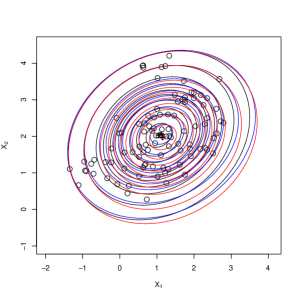
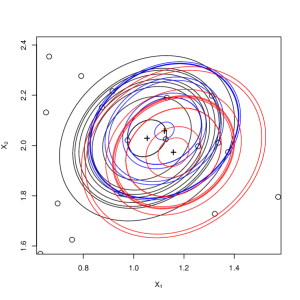
The Mahalanobis distance is also illustrated. One sample of size $n=100$ was simulated from the bivariate normal distribution with the above parameters. Afterwards, the Mahalanobis distances $d_{ii}=(X_{i}-\bar{X})^{T}S_{n}^{-1}(X_{i}-\bar{X}),\ i=1,\ldots,n$ were calculated. They represent $n$ co-axial ellipses centered at $\bar{X}$ - see Figure 3 (black ellipses). The modified Mahalanobis distances replaced $\bar{X}$ by the affine-equivariant trimmed $\mathbf{L}_{n1}$-estimator with $k_{n}=15$ (see the blue ellipses on Figure 3) and affine-equivariant $\mathbf{L}_{n2}$-estimator (see the red ellipses on Figure 3) with analogous modification of $S_{n}$.

Table 1. Normal distribution: The mean in the sample of 5 000 replications of estimators $\mathbf{L}_{n1}$ (trimmed) and $\mathbf{L}_{n2},$ sample sizes $n=100$

i	${\mathbf{L}}_{n1}^{(i)}$			$\mathbf{L}_{n2}^{(i)}$
1	0.999607	2.001435	-0.998297	0.999401	1.999796	-0.999943
2	0.999473	2.001423	-0.996185	0.999083	1.999584	-0.999782
3	0.999519	2.000290	-0.993274	0.998926	1.999509	-0.999801
4	0.999435	2.000190	-0.991901	0.998854	1.999496	-0.999871
5	0.999474	2.000771	-0.991295	0.998811	1.999476	-0.999973
6	0.999646	2.001285	-0.990964	0.998781	1.999471	-1.000032
7	0.999926	2.001519	-0.990829	0.998773	1.999470	-1.000049
8	0.999952	2.001529	-0.990803	0.998772	1.999472	-1.000068
9	0.999939	2.001497	-0.990745	0.998775	1.999489	-1.000071
10	0.999853	2.001424	-0.990711	0.998779	1.999497	-1.000061

Figure 1: Normal distribution: Box-plots of the 5 000 estimated values of $\theta_{1}(=1)$ (top), $\theta_{2}(=2)$ (middle) and $\theta_{3}(=-1)$ (bottom) for the $\mathbf{L}_{n1}^{(1)}$, $\mathbf{L}_{n1}^{(5)}$, $\mathbf{L}_{n1}^{(10)}$, $\mathbf{L}_{n2}^{(1)}$, $\mathbf{L}_{n2}^{(5)}$, $\mathbf{L}_{n2}^{(10)}$, mean and median.

Table 2. Normal distribution: The mean, median and minimum of D-efficiency in the sample of 5 000 replications of estimators $\mathbf{L}_{n1}$ (trimmed) and $\mathbf{L}_{n2},$ sample sizes $n=100$
${\mathbf{L}}_{n1}^{(i)}$ $\mathbf{L}_{n2}^{(i)}$ iterration mean median minimum mean median minimum 2 1.000637 0.999615 0.871029 0.999862 0.999670 0.951057 3 1.001272 0.998593 0.818591 0.999625 0.999451 0.946809 4 1.001106 0.997822 0.793030 0.999392 0.999231 0.946575 5 1.000697 0.997283 0.794157 0.999205 0.999041 0.946332 6 1.000394 0.997211 0.793903 0.999078 0.998886 0.946022 7 1.000131 0.997122 0.793903 0.998997 0.998802 0.945613 8 0.999916 0.996964 0.793903 0.998951 0.998807 0.945032 9 0.999882 0.996924 0.793903 0.998921 0.998768 0.944518 10 0.999860 0.996924 0.793903 0.998899 0.998706 0.944272

Table 3. Normal distribution: The 25%-quantile, 75%-quantile and max of D-efficiency in the sample of 5000 replications of estimators $\mathbf{L}_{n1}$ (trimmed) and $\mathbf{L}_{n2},$ sample sizes $n=100$
${\mathbf{L}}_{n1}^{(i)}$ $\mathbf{L}_{n2}^{(i)}$ iteration 25%-quantile 75%-quantile max 25%-quantile 75%-quantile max 2 0.971669 1.028444 1.169137 0.990914 1.008819 1.057115 3 0.960891 1.039437 1.295245 0.989675 1.009489 1.065753 4 0.956068 1.042774 1.294952 0.989358 1.009426 1.068542 5 0.953186 1.043542 1.301147 0.989098 1.009239 1.069236 6 0.952193 1.044435 1.305327 0.989000 1.009182 1.069437 7 0.951535 1.044942 1.326996 0.988916 1.009142 1.069600 8 0.951441 1.044394 1.330791 0.988839 1.009109 1.069226 9 0.951452 1.044562 1.330791 0.988802 1.009087 1.069236 10 0.951356 1.044749 1.330791 0.988771 1.009062 1.069278

Figure 2: Normal distribution: Box-plots of the 5 000 estimated values of D-efficiency for the $\mathbf{L}_{n1}^{(2)}$, $\mathbf{L}_{n1}^{(5)}$, $\mathbf{L}_{n1}^{(10)}$, $\mathbf{L}_{n2}^{(2)}$, $\mathbf{L}_{n2}^{(5)}$, $\mathbf{L}_{n2}^{(10)}$.

Figure 3: Normal distribution: Mahalanobis distances represented by co-axial ellipses centered at the mean $\bar{X}$ (black), at the trimmed $\mathbf{L}_{n1}$-estimator (blue) and at the $\mathbf{L}_{n2}$-estimator (red). All simulated bivariate data with the every tenth contour are illustrated on the left, detail of the center with the first ten contours is on the right.

3.2 Multivariate t-distribution

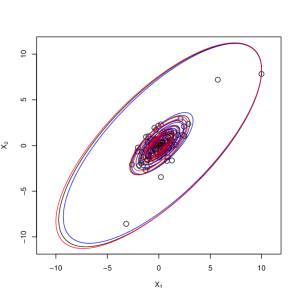
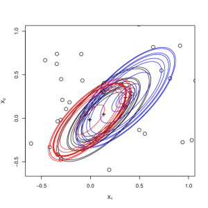
Similarly, we illustrate the procedure on samples of size $n=100$ simulated from the multivariate $t$ distribution with 3 degree of freedom $t_{3}(\mbox{\boldmath$\theta$},\mbox{\boldmath$\Sigma$}),$ with the same parameters as in (12). Each time, 10 iterations of affine-equivariant trimmed $\mathbf{L}_{n1}$-estimator ($k_{n}=15$) and of affine-equivariant $L_{n2}$-estimator, started from the initial estimator, were calculated. 5 000 replications of the model were simulated and the mean was computed, for the sake of comparison. Results are summarized in Table 4. Figure 4 illustrates the distribution of estimated parameters $\theta_{1}$, $\theta_{2},$ $\theta_{3}$ for various iterations of $\mathbf{L}_{n1}$-estimator and $\mathbf{L}_{n2}$-estimator and compares them with the mean and median. The Tables 5-6 and Figure 5 compare the D-efficiencies of the proposed estimators and Figure 6 illustrates the Mahalanobis distances.

Table 4. $t$-distribution: The mean in the sample of 5 000 replications of estimators $\mathbf{L}_{n1}$ (trimmed) and $\mathbf{L}_{n2},$ sample sizes $n=100$

i	${\mathbf{L}}_{n1}^{(i)}$			$\mathbf{L}_{n2}^{(i)}$
1	1.004760	2.002252	-0.992618	1.003081	2.001199	-0.998781
2	1.005034	2.001851	-0.991150	1.002154	2.000044	-0.999996
3	1.005473	2.001430	-0.991330	1.001744	1.999661	-1.000627
4	1.005334	2.000732	-0.992535	1.001594	1.999526	-1.000909
5	1.005351	2.000951	-0.993532	1.001540	1.999475	-1.001028
6	1.005007	2.001127	-0.994361	1.001528	1.999452	-1.001069
7	1.004636	2.001009	-0.994817	1.001522	1.999447	-1.001086
8	1.004520	2.000930	-0.995011	1.001524	1.999443	-1.001090
9	1.004466	2.000911	-0.995172	1.001526	1.999442	-1.001090
10	1.004445	2.000821	-0.995221	1.001527	1.999444	-1.001086

Table 5. $t$-distribution: The mean, median and minimum of D-efficiency in the sample of 5 000 replications of estimators $\mathbf{L}_{n1}$ (trimmed) and $\mathbf{L}_{n2},$ sample sizes $n=100$
${\mathbf{L}}_{n1}^{(i)}$ $\mathbf{L}_{n2}^{(i)}$ iterration mean median minimum mean median minimum 2 1.001813 1.000857 0.896048 1.000812 1.000303 0.857210 3 1.001827 1.001157 0.824105 1.000556 1.000109 0.845643 4 1.001377 1.000619 0.810082 1.000360 0.999912 0.844578 5 1.000887 0.999840 0.796776 1.000260 0.999766 0.844182 6 1.000372 0.999121 0.777458 1.000214 0.999723 0.843850 7 1.000024 0.999086 0.756777 1.000196 0.999740 0.843933 8 0.999881 0.998921 0.756555 1.000187 0.999714 0.843928 9 0.999806 0.998907 0.756655 1.000184 0.999726 0.843917 10 0.999753 0.998921 0.756655 1.000183 0.999726 0.843897

Table 6. $t$-distribution: The 25%-quantile, 75%-quantile and max of D-efficiency in the sample of 5 000 replications of estimators $\mathbf{L}_{n1}$ (trimmed) and $\mathbf{L}_{n2},$ sample sizes $n=100$
${\mathbf{L}}_{n1}^{(i)}$ $\mathbf{L}_{n2}^{(i)}$ iterration 25%-quantile 75%-quantile max 25%-quantile 75%-quantile 2 0.980004 1.023251 1.157852 0.986053 1.014785 1.194658 3 0.972157 1.030707 1.212343 0.983882 1.016369 1.212103 4 0.967982 1.032541 1.214165 0.983518 1.016634 1.214597 5 0.967034 1.032940 1.222945 0.983380 1.016629 1.215499 6 0.966116 1.032850 1.260563 0.983366 1.016565 1.215862 7 0.965784 1.032895 1.261640 0.983391 1.016572 1.216013 8 0.965561 1.032746 1.261675 0.983406 1.016537 1.216332 9 0.965436 1.032643 1.261675 0.983380 1.016522 1.216431 10 0.965404 1.032680 1.261675 0.983406 1.016522 1.216579

Although $L_{n}^{(1)}$ resembles the NN-estimator, its behavior for $t$-distribution reveals its robustness no less than $L_{n}^{(2)}.$ For multivariate normal distribution, both $L_{n}^{(1)}$ and $L_{n}^{(2)}$ seem to be doing well against outliers. Figures 4 and 5 illustrate this feature in a visible way.

Figure 4: $t$-distribution: Box-plots of the 5 000 estimated values of $\theta_{1}(=1)$ (top), $\theta_{2}(=2)$ (middle) and $\theta_{3}(=-1)$ (bottom) for the $\mathbf{L}_{n1}^{(1)}$, $\mathbf{L}_{n1}^{(5)}$, $\mathbf{L}_{n1}^{(10)}$, $\mathbf{L}_{n2}^{(1)}$, $\mathbf{L}_{n2}^{(5)}$, $\mathbf{L}_{n2}^{(10)}$, mean and median.

Figure 5: $t$-distribution: Box-plots of the 5 000 estimated values of D-efficiency for the $\mathbf{L}_{n1}^{(2)}$, $\mathbf{L}_{n1}^{(5)}$, $\mathbf{L}_{n1}^{(10)}$, $\mathbf{L}_{n2}^{(2)}$, $\mathbf{L}_{n2}^{(5)}$, $\mathbf{L}_{n2}^{(10)}$.

Figure 6: $t$-distribution: Mahalanobis distances represented by co-axial ellipses centered at the mean $\bar{X}$ (black), at the trimmed $\mathbf{L}_{n1}$-estimator (blue) and at the $\mathbf{L}_{n2}$-estimator (red). All simulated bivariate data with the every tenth contour are illustrated on the left, detail of the center with the first ten contours is on the right.

References

• (1) Chaubey, Y.P. and Sen, P. K.: On smooth estimation of survival and density functions. Statistics and Decisions 14, 1–22 (1996)
• (2) Chakraborty, B.: On affine equivariant multivariate quantiles. Ann. Inst. Statist. Math. 53, 380–403 (2001)
• (3) Chernoff, H. and Teicher, H. A central limit theorem for sums of interchangeable random variables. Ann. Math. Statist. 29, 118–130 (1958)
• (4) Critchley, F., Lu, G. and Atkinson, R. A. Envelope plots of ordered Mahalanobis distances: Uses and efficient generation. The Open University, Technical Report 05/09 (2005)
• (5) Eaton, M. Multivariate Statistics. Wiley, New York (1983)
• (6) Hallin, M., Paindaveine, D. and Šíman, M.: Multivariate quantiles and multiple-output regression quantiles: From L1 optimization to halfspace depth. Ann. Statist. 38, 635- 669 (2010)
• (7) Hoeffding, W.: Probability inequalities for sums of bounded random variables. J. Amer. Statist. Assoc. 58, 13–30 (1963)
• (8) Jurečková, J., Sen, P. K., Picek, J.: Methodology in Robust and Nonparametric Statistics. Chapman & Hall/CRC, Boca Raton (2013)
• (9) Kong, L. and Mizera, I.: Quantile tomography: Using quantiles with multivariate data. Statistica Sinica 22, 1589–1610 (2012)
• (10) Liu, R. Y., Parelius, J. M. and Singh, K.: Multivariate analysis by data depth: Descriptive statistics, graphics and inference. Ann. Statist. 27, 783–858 (1999)
• (11) Lopuhaa¨¨a\ddot{\rm a}, H. P. and Rousseeuw, P. J.: Breakdown points of affine equivariant estimators of multivariate location and covariance matrices. Ann. Statist. 19, 229–248 (1991)
• (12) Obenchain, R.L.: Multivariate procedures invariant under linear transformations. Ann. Math. Statist. 42, 1569 -1578 (1971)
• (13) Oja, H.: Multivariate Nonparametric Methods with R. An Approach Based on Spatial Signs and Ranks. Lecture Notes in Statistics 199, Springer, New York (2010)
• (14) Roelant, E. and Van Aelst, S.: An L1-type estimator of multivariate location and shape. Statistical Methods and Applications 15, 381–393 (2007)
• (15) Sen, P. K.: On some properties of rank-weighted means. J. Indian. Soc. Agric. Statist. 16, 51–61 (1964)
• (16) Serfling, R. J.: Equivariance and invariance properties of multivariate quantile and related functions, and the role of standardization. J. Nonparametric Statist. 22, 915–936 (2010)
• (17) Weber, N. C.: A martingale approach to central limit theorems for exchangeable random variables. Journal of Applied Probability 17, 662–673 (1980)
• (18) Zuo, Y.: Projection-based depth functions and associated medians. Ann. Statist. 31, 1460- 1490 (2003)
• (19) Zuo, Y.: Projection-based affine equivariant multivariate location estimators with the best possible finite sample breakdown point. Statistica Sinica 14, 1199–2008 (2004)
• (20) Zuo, Y.: Multidimensional trimming based on projection depth. Ann. Statist. 34, 2211- 2251 (2006).
• (21) Zuo, Y., Cui, H. and He, X.: On the Stahel-Donoho estimator and depth-weighted means of multivariate data. Ann. Statist. 32, 167–188 (2004)