Age-Specific Mortality and Fertility Rates for Probabilistic Population Projections

Abstract

The UN released official probabilistic population projections (PPP) for all countries for the first time in July 2014. These were obtained by projecting the period total fertility rate (TFR) and life expectancy at birth ($e_{0}$) using Bayesian hierarchical models, yielding a large set of future trajectories of TFR and $e_{0}$ for all countries and future time periods to 2100, sampled from their joint predictive distribution. Each trajectory was then converted to age-specific mortality and fertility rates, and population was projected using the cohort-component method. This yielded a large set of trajectories of future age- and sex-specific population counts and vital rates for all countries. In this paper we describe the methodology used for deriving the age-specific mortality and fertility rates in the 2014 PPP, we identify limitations of these methods, and we propose several methodological improvements to overcome them. The methods presented in this paper are implemented in the publicly available bayesPop R package.

Keywords: Bayesian hierarchical model; Cohort-component method; Life expectancy at birth; Markov chain Monte Carlo; Total fertility rate; United Nations; World Population Prospects.

1 Introduction

The United Nations released official probabilistic population projections for all countries for the first time in July 2014 (Gerland et al., 2014). They were produced by probabilistically projecting the period total fertility rates (TFR) and life expectancies ($e_{0}$) for all countries using Bayesian hierarchical models (Alkema et al., 2011; Raftery et al., 2013). These probabilistic projections took the form of a large set of trajectories, each of which was sampled from the joint predictive distribution of TFR and female and male $e_{0}$ for all countries and all future time periods to 2100 using Markov chain Monte Carlo (MCMC) methods .

For each trajectory, the life expectancies were converted to age- and sex-specific mortality rates, and the total fertility rates were converted to age-specific fertility rates. The population was then projected forward using the cohort-component method. This yielded a large set of trajectories of population by age and sex, and age-specific fertility and mortality rates, for all countries and future time periods jointly. These were summarized by predictive medians and 80% and 95% prediction intervals for a wide range of population quantities of interest, for all countries and a wide range of regional and other aggregates. They were published as the UN’s Probabilistic Population Projections (PPP), and are available at http://esa.un.org/unpd/ppp.

This paper focuses on the methods used to convert probabilistic projections of $e_{0}$ and TFR to probabilistic projections of age-specific mortality and fertility rates. Some limitations of the methods used for the 2014 PPP are identified, and several improvements are proposed to overcome them. The methods presented in this paper are implemented in an open source R package called bayesPop (Ševčíková & Raftery, 2014; Ševčíková et al., 2014).

The paper is organized as follows. In Section 2 we describe the current method in PPP for projecting age-specific mortality rates and our proposed improvements. In Section 2.1 we outline the Probabilistic Lee-Carter method used in the 2014 PPP. In the rest of Section 2 we propose several improvements to overcome limitations of this method. These include a new Coherent Kannisto Method for joint projection of future age-specific mortality rates at very high ages that avoids unrealistic crossovers between the sexes (Section 2.2), application of the Coherent Lee-Carter method to avoid crossovers at lower ages (Section 2.3), new methods for avoiding jump-off bias (Section 2.4), and application of the Rotated Lee-Carter method to reflect the fact that when mortality rates are low, they tend to decline faster at older than at younger ages (Section 2.5). In Section 3, we describe the current method in PPP for projecting age-specific fertility rates and our proposed improvements. We conclude with a discussion in Section 4.

2 Age-Specific Mortality Rates for Probabilistic Population Projections

2.1 Probabilistic Lee-Carter Method

Our methodology is based on the Lee-Carter model (Lee & Carter, 1992):

$$\log[m_{x}(t)]=a_{x}+b_{x}k(t)+\varepsilon_{x}(t),\quad\varepsilon_{x}(t)\sim N(0,\sigma_{\varepsilon}^{2}),$$

where $m_{x}(t)$ is the mortality rate for age $x$ and time period $t$. The quantity $a_{x}$ represents the baseline pattern of mortality by age over time, and $b_{x}$ is the average rate of change in mortality rate by age group for a unit change in the mortality index $k(t)$. The parameter $k(t)$ is a time-varying index of the overall level of mortality, and $\varepsilon_{x}(t)$ is the residual at age $x$ and time $t$. Throughout this paper, $\log$ denotes the natural logarithm.

For a given matrix of rates $m_{x}(t)$ the model is estimated by a least squares method. The baseline mortality pattern $a_{x}$ is estimated as the average of $\log[m_{x}(t)]$ over the past time periods with observed data. Since the model is underdetermined, $b_{x}$ is identified by setting $\sum_{x}b_{x}=1$, where the sum is over all ages or age groups $x$. Also, $k(t)$ is identified by setting $\sum_{t=1}^{T}k(t)=0$, where $T$ is the number of past time periods for which data are available. The estimates are then

$$\hat{a}_{x} = \frac{\sum_{t=1}^{T}\log[m_{x}(t)]}{T}$$ (1)

$$\hat{k}(t) = \sum_{x}\left\{\log[m_{x}(t)]-\hat{a}_{x}\right\}$$ (2)

$$\hat{b}_{x} = \frac{\sum_{t=1}^{T}\left\{\log[m_{x}(t)]-\hat{a}_{x}\right\}\hat{k}(t)}{\sum_{t=1}^{T}\hat{k}(t)^{2}}.$$ (3)

To forecast $m_{x}(t)$, one needs to project $k(t)$ into the future. To project $k(t)$, the Lee-Carter method uses a random walk with drift:

$$\hat{k}(t+1)=\hat{k}(t)+\hat{d},\quad\text{where}\;\hat{d}=\frac{1}{T-1}[\hat{k}(T)-\hat{k}(1)].$$

Lee & Miller (2001) proposed replacing the step of projecting $k(t)$ by itself by matching future $k(t)$ to future projected $e_{0}(t)$.

Current calculations are done using a highest age or open interval of 85$+$. For projections one needs to extend mortality rates to higher ages $x$, usually beyond $100+$, because mortality rates are expected broadly to decline over time in the future, so there will be larger numbers of people at higher ages. For extending the force of mortality at older age groups, the Kannisto model provides a robust way to fit available mortality rates from age 80 to 100, and to extrapolate mortality rates up to age 130 in a way that is consistent with empirical observations on oldest-old mortality (Thatcher et al., 1998).

The Bayesian probabilistic projections of life expectancy (Raftery et al., 2013; Raftery et al., 2014) provide us with a set of future trajectories of female and male $e_{0}$, representing a sample from the joint predictive distribution of future female and male $e_{0}$ for all countries and all future time periods. The 2014 PPP used methods for turning a trajectory of future $e_{0}$ values into a set of future age-specific mortality based on the ideas of Lee & Miller (2001) and Li & Gerland (2011); see Raftery et al. (2012). They were based on the following algorithm:

Algorithm 1

Let $t\in\{1,\ldots,T\}$ and $\tau\in\{T+1,\dots,T_{p}\}$ denote the observed and projected time periods, respectively.

1. Using the Kannisto method extend $m_{x}(t)$ to higher age groups so that $\max(x)=130+$ for all $t$.

2. Estimate $a_{x}$, $k(t)$ and $b_{x}$ using the extended historical $m_{x}(t)$ (equations 1–3).

3. For a given $e_{0}(\tau)$ in each trajectory and given $a_{x}$ and $b_{x}$, solve for future $k(\tau)$ numerically using life tables. This yields a nonlinear equation which can be solved using the bisection method. More details are given in Section 2.6.

4. Compute mortality rates by $\log[m_{x}(\tau)]=\hat{a}_{x}+\hat{b}_{x}k(\tau)$ for each trajectory and future time $\tau$.

Applying these steps to all trajectories of $e_{0}$ yields a posterior predictive distribution of $m_{x}(t)$.

However, this procedure has a number of drawbacks. There is no assurance that the extension of $m_{x}(t)$ to higher ages yields mortality rates that are coherent between males and females. Similarly, the predicted $m_{x}(\tau)$ can lead to unwanted crossovers between female and male mortality rates, since they are obtained independently for each sex. In the following sections, we present solutions to these and other limitations of the simple algorithm above, and give more details about Step 3.

2.2 Coherent Kannisto Method

A sex-independent extension of the observed mortality rates to higher age categories can lead to unrealistic crossovers at higher ages. We propose a modification of the Kannisto method that treats male and female mortality rates jointly. In this section, for simplicity we omit the time index $t$.

The original Kannisto model has the form

$$m_{x} = \frac{ce^{dx}}{1+ce^{dx}}e^{\varepsilon_{x}},\;\mbox{ or }$$

$$\text{logit}(m_{x}) = \log c+dx+\varepsilon_{x},$$

where $\varepsilon_{x}$ is a random perturbation with mean zero. The model is usually estimated independently for each sex, assuming independence across ages and normality of the $\varepsilon_{x}$, using a maximum likelihood method (Thatcher et al., 1998; Wilmoth et al., 2007). This yields sex-specific parameter estimates $\hat{d}_{M}$, $\hat{d}_{F}$, $\hat{c}_{M}$, $\hat{c}_{F}$.

We suggest modifying this by forcing the sex-specific parameters $d_{M}$ and $d_{F}$ to be equal (i.e. $d_{M}=d_{F}=d$), but still allowing the parameters $c_{M}$ and $c_{F}$ to differ between the sexes:

$$\text{logit}(m_{x}^{g})=\log c_{g}+dx+\varepsilon_{x}^{g},\quad\mbox{ for }\;g=M,F.$$

This leads to the following model:

$$\text{logit}(m_{x}^{g})=\beta_{0}+\beta_{1}1_{(g=M)}+\beta_{2}x+\varepsilon_{x}^{g},$$

where $1_{(g=M)}=1$ if $g=M$ and 0 otherwise.

To estimate the $\beta$ parameters, we fit the model to the observed $m_{x}$ for ages 80–99 by ordinary least-squares regression, which corresponds to maximum likelihood under the assumptions of independence and normality of the $\varepsilon_{x}^{g}$. There are four age groups in the data used for fitting the model, and thus eight points in total for both sexes. Then,

$$\hat{c}_{F} = e^{\hat{\beta}_{0}},$$

$$\hat{c}_{M} = e^{\hat{\beta}_{0}+\hat{\beta}_{1}},$$

$$\hat{d} = \hat{\beta}_{2}.$$

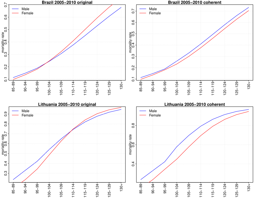
Figure 1 shows the resulting $m_{x}$ for old ages for Brazil and Lithuania in the last observed time period. From the left panels we see that there are crossovers using the classic Kannisto method, which is unrealistic. However, male mortality stays above female mortality in the coherent version, as can be seen in the right panels; this is more realistic.

Figure 1: Mortality rates for male (blue) and female (red) extended using the coherent Kannisto method (right panels) compared to original Kannisto (left panels) for Brazil and Lithuania in the last observed time period (2005-2010).

2.3 Coherent Lee-Carter Method

We will adopt an extension of the Lee-Carter method suggested by Li & Lee (2005), the so-called coherent Lee-Carter method. It takes into account the fact that mortality patterns for closely related populations are expected to be similar. In our application, these related populations will be males and females in the same country, since there is no expectation that the life expectancy will diverge between such groups. Thus, the Lee-Carter method is extended by two requirements:

$$b_{x}^{M} = b_{x}^{F},$$

$$k_{M}(\tau) = k_{F}(\tau),$$ (4)

where $M$ and $F$ denotes male and female sex, respectively. This ensures that the rates of change of the future mortality rates are the same for the two sexes, and thus avoids crossovers.

2.4 Avoiding Jump-off Bias

Mortality rates in the last period of the historical data used for estimation (or jump-off period) are commonly referred to as jump-off rates (Booth et al., 2006). Often there is a mismatch between fitted rates for the last period $T$ and the actual rates (jump-off bias). As a result, a discontinuity between the actual rates in the jump-off period and the rates projected in the first projection period may occur.

A possible solution to avoid jump-off bias is to constrain the model in such a way that $k(t)$ passes through zero in the jump-off period $T$, and to use $m_{x}$ only from the last fitting period to obtain $a_{x}$ (Lee & Miller, 2001):

$$a_{x} = \log[m_{x}(T)]\implies k(T)=0.$$ (5)

A disadvantage of this solution is that in cases where the mortality rates are bumpy in the jump-off period (i.e. not smooth across ages), this “bumpiness” propagates into the future. In general for projections, we suggest using the age-specific mortality rates from the last fitting period and smoothing them over age if necessary (e.g. for small populations with few deaths in some age groups) while preserving the value for the youngest age group:

$$a_{x} = \text{smooth}_{x}\{\log[m_{x}(T)]\}\;\text{ with }\;a_{0-1}=\log[m_{0-1}(T)].$$ (6)

Figure 2 shows the resulting difference in $\log[m_{x}(\tau)]$ projected to $\tau=2095-2100$ for two countries using the three different methods of computing $a_{x}$, namely equations (1), (5) and (6). As can be seen in the case of Bangladesh, the smoothing step removes bumps whereas the averaging method does not.

Figure 2: Log female mortality rates for Bangladesh and Pakistan in 2095-2100 projected using three different methods for computing $a_{x}$: (1) using an average $m_{x}$ over time (blue line); (2) using the latest smoothed $m_{x}$ (red line); and (3) using the latest $m_{x}$ as it is (grey line).

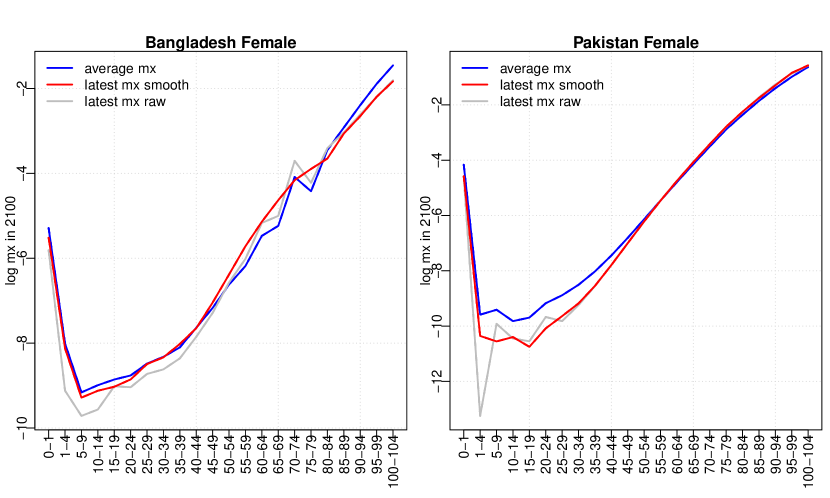
Figure 3 shows the impact of the methods on $m_{x}$ as time series for Bangladesh for three different age groups. Using the average $m_{x}$ results in jump-offs for the 5–9 and 95–99 age groups (blue curve). If the latest raw $m_{x}$ are used, the jump-offs are eliminated (grey curve). A smoothed version creates a new jump-off for the age group 75–79 (red curve).

Figure 3: Mortality rates for Bangladesh by time for three different age groups. Colors correspond to the same methods as in Figure 2.

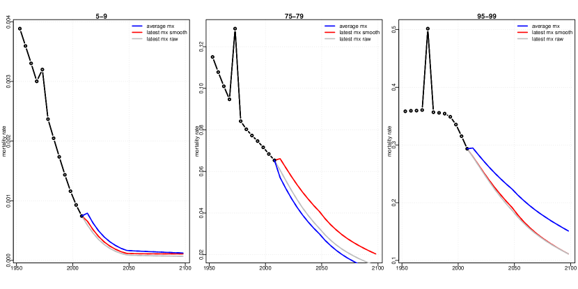
This shows that there is a trade-off between bumpy mortality rates over ages in later projection years and no jump-offs, and smooth mortality rates with no jump-offs. Our solution is to decide on a country-specific basis which method is more appropriate.

2.5 Rotated Lee-Carter Method

Li et al. (2013) focused on the fact that in more developed regions, once countries have already reached a high level of life expectancy at birth, the mortality decline decelerates at younger ages and accelerates at old ages. This change in the pace of mortality decline by age cannot be captured by the original Lee-Carter method, since this constrains the rate of change $b_{x}$ to be constant over time. They proposed instead rotating the $b_{x}$ over time to a so-called ultimate $b_{x}$, denoted by $b_{u,x}$, which is computed as follows.

Let

$$\bar{b}_{15-64}=\frac{1}{10}\sum_{x=15-19}^{60-64}b_{x}\,.$$

Then

$$b_{u,x} = \left\{\begin{array}[]{ll}\bar{b}_{15-64}&\text{ for }\;x\in\{0-1,1-4,5-9,\dots,60-64\},\\ b_{x}\cdot b_{u,60-64}/b_{65-70}&\text{ for }\;x\in\{65-70,\dots,130+\},\end{array}\right.$$ (9)

with $b_{u,x}$ scaled to sum to unity over all ages.

The rotation is dependent on $e_{0}(\tau)$, and so the resulting $b_{x}$ also becomes time-dependent. The rotation finishes at a certain level of live expectancy, denoted by $e_{0}^{u}$. Li et al. (2013) recommend using $e_{0}^{u}=102$. Using the smooth weight function

$$w(\tau) = \left\{\frac{1}{2}\left[1+\sin[\frac{\pi}{2}(2w^{\prime}(\tau)-1)]\right]\right\}^{\frac{1}{2}}\quad\text{with}\quad w^{\prime}(\tau)=\frac{e_{0}(\tau)-80}{e_{0}^{u}-80},$$

the rotated $b_{x}$ at time $\tau$, denoted by $B_{x}(\tau)$, is derived as:

$$B_{x}(\tau) = \left\{\begin{array}[]{lc}b_{x},&e_{0}(\tau)<80,\\ \left[1-w(\tau)\right]b_{x}+w(\tau)b_{u,x},&80\leq e_{0}(\tau)<e_{0}^{u},\\ b_{u,x},&e_{0}(\tau)\geq e_{0}^{u}.\end{array}\right.$$ (13)

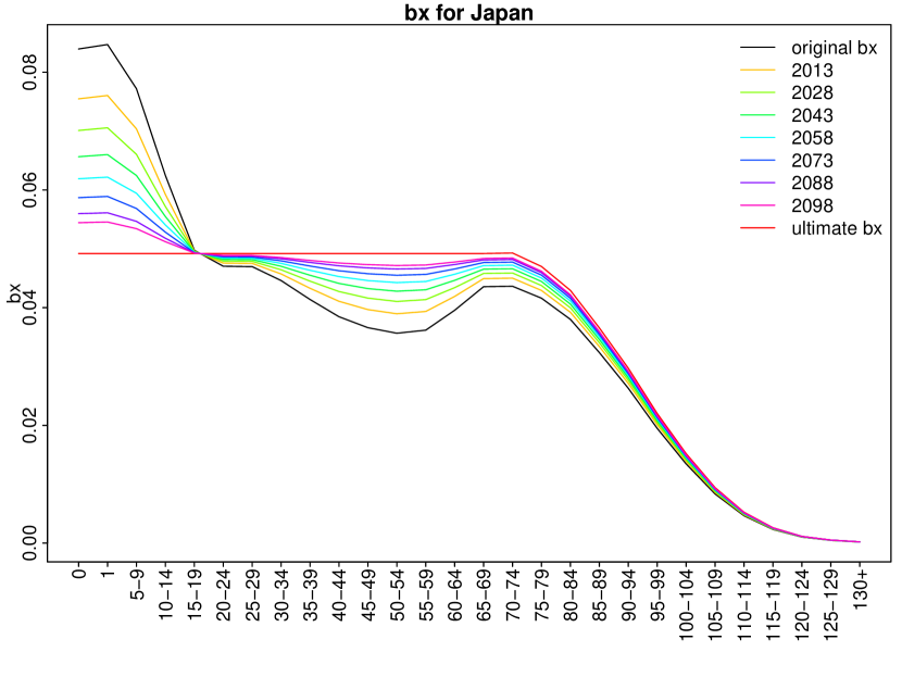
Figure 4 shows the results for Japan as an example. The original $b_{x}$ is shown by the black curve. The ultimate $b_{u,x}$, to be reached at life expectancy of 102, is in red. The remaining curves show the change over time starting with yellow and continuing towards the red curve.

Figure 4: Rotating the parameter $b_{x}$ over time. The original $b_{x}$ (black curve) approaches the ultimate $b_{u,x}$ (red curve) over time starting with yellow and continuing towards the darker colors.

2.6 Computing Life Tables

Step 3 in Algorithm 1 calls for matching future $k(\tau)$ to projected $e_{0}(\tau)$. This is a nonlinear equation in $k(\tau)$. It is solved by an iterative nonlinear procedure in which for given values of $a_{x}$, $b_{x}$ and $k(\tau)$ a life table is produced, and the resulting life expectancy is computed and compared with the projected $e_{0}(\tau)$. We used a bisection method to solve the nonlinear equation. This is simple and robust and involves relatively few iterations. It would be possible to use a nonlinear solution method that is more efficient computationally, but the computational gains would be modest and this could make the method much more complex.

In the process of computing life tables, the conversion of mortality rates $m_{x}(\tau)$ to probabilities of dying $q_{x}(\tau)$ follows the approach used by the United Nations to compute abridged life tables. This is computed by the LIFTB function in Mortpak (United Nations, 1988, 2013a), where at a given time point the probability of dying for an individual between age $x$ and $x+n$ is:

$${}_{n}{q_{x}} = \frac{n*\tensor[_{n}]{m}{{}_{x}}}{1+(n-\tensor[_{n}]{A}{{}_{x}})*\tensor[_{n}]{m}{{}_{x}}},$$ (14)

with $n$ being the length of the age interval and ${}_{n}{A_{x}}$ being the average number of years lived between ages $x$ and $x+n$ by those dying in the interval. With $l_{x}$ being the number of survivors at age $x$, we have

$${l_{x+n}} = {l_{x}}{(1-\tensor[_{n}]{q}{{}_{x}})},$$ (15)

$${}_{n}{d_{x}} = {{l_{x}}-{l_{x+n}}},$$ (16)

$${}_{n}{L_{x}} = {{}_{n}{A_{x}}{l_{x}}-{(n-\tensor[_{n}]{A}{{}_{x}})l_{x+n}}},$$ (17)

where $\tensor[_{n}]{d}{{}_{x}}$ denotes the number of deaths between ages $x$ and $x+n$ and $\tensor[_{n}]{L}{{}_{x}}$ denotes the number of person-years lived between ages $x$ and $x+n$. The expectation of life at age $x$ (in years) $e_{x}$ is given by

$${e_{x}}=\frac{T_{x}}{{l}_{x}}\quad\text{with}\quad{T_{x}}=\sum_{a=x}^{\infty}{{}_{n}}{L}{{}_{a}},$$

where $T_{x}$ is the number of person-years lived at age $x$ and older.

For ages 15 and over, the expression for ${}_{n}{A_{x}}$ is derived from the Greville (1943) approach to calculating age-specific separation factors based on the age pattern of the mortality rates themselves with:

$${}_{n}{A_{x}}=2.5-\frac{25}{12}(_{n}{m_{x}}-k),\quad\text{where}\;k=\frac{1}{10}\log\left(\frac{\tensor[_{n}]{m}{{}_{x+5}}}{\tensor[_{n}]{m}{{}_{x-5}}}\right).$$

For ages 5 and 10, ${}_{n}{A_{x}}=2.5$ and for ages under 5, values from the Coale and Demeny West region relationships are used for ${}_{n}{A_{x}}$ (Coale & Demeny, 1966).

2.7 Summary of Improved Algorithm

We now summarize the modifications described in the previous sections by proposing an improved algorithm for deriving the age-specific mortality rates $m_{x}$ for potential use in future probabilistic population projections.

Algorithm 2

As before, let $t\in\{t_{1},\dots,T\}$ and $\tau\in\{T+1,\dots T_{p}\}$ denote the observed and projected time periods, respectively. Also, let $g\in\{F,M\}$ be an index to distinguish sex-specific measures.

1. Using the Coherent Kannisto Method from Section 2.2, extend $m_{x}(t)$ to higher age categories with $\max(x)=130+$ for all $t$.

2. Choose a method to estimate $a_{x}$, i.e. one of equations (1), (5) or (6), depending on country specifics. Do the estimation for each sex $g$, obtaining $a_{x}^{g}$.

3. Estimate $k(t)$ and $b_{x}$ using the extended historical $m_{x}(t)$ and equations (2–3) for $g=M,F$ independently, yielding $b_{x}^{g}$.

4. Given $b_{x}^{M}$ and $b_{x}^{F}$ from Step 3, set $b_{x}=\frac{b_{x}^{M}+b_{x}^{F}}{2}$.

5. Compute the ultimate $b_{ux}$ as in equation (9).

6. For a combined $e_{0}(\tau)=\left[e_{0}^{M}(\tau)+e_{0}^{F}(\tau)\right]/2$ in each trajectory, compute $B_{x}(\tau)$ as in equation (13).

7. For a given sex-specific $e_{0}^{g}(\tau)$ in each trajectory and given $a_{x}^{g}$ and $B_{x}(\tau)$, solve for future $k_{g}(\tau)$ numerically using life tables. This yields a nonlinear equation which is solved using the bisection method, as described in Section 2.6.

8. For each trajectory, time $\tau$ and sex $g$, compute mortality rates by $\log[m_{x}^{g}(\tau)]=a_{x}^{g}+B_{x}(\tau)k_{g}(\tau)$.

9. Since the previous step does not comply with equation (4) and thus can lead to crossovers in high ages, an additional constraint is added:
   If $e_{0}^{M}(\tau)<e_{0}^{F}(\tau)$ then

   $$m_{x}^{M}(\tau) = \max[m_{x}^{M}(\tau),m_{x}^{F}(\tau)]\text{ for }x\geq 100.$$

Figure 5: Probabilistic projection of age-specific mortality rates for Japan (left panel) and Kazakhstan (right panel) in the time period 2095-2100. Both plots show the marginal distribution for male (blue lines) and female (red lines) where the dashed lines mark the 80% probability intervals and the solid lines are 20 randomly sampled trajectories (out of 1000) for each sex. The $y$-axis is on the logarithmic scale.

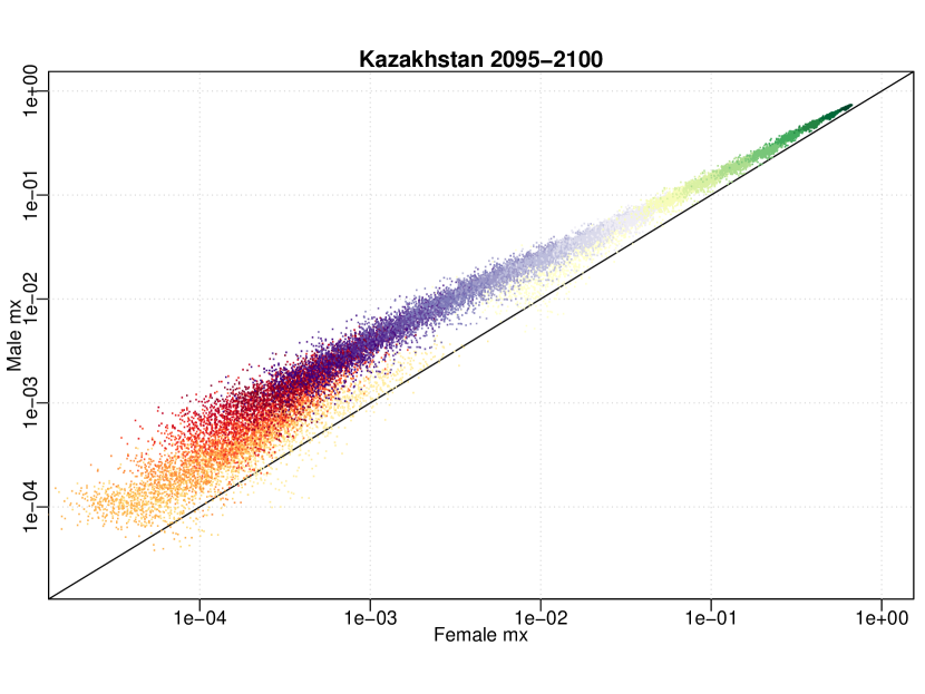
Figure 5 shows the resulting probabilistic projection of $m_{x}(\tau)$ for the period 2095-2100 for both sexes in two selected countries. In addition to the marginal distribution for Kazakhstan in the right panel of Figure 5, its joint distribution for males and females is shown in Figure 6 on a logarithmic scale. Points below the $x=y$ solid line indicate crossovers in the individual trajectories. It can be seen that only a few trajectories experience crossovers when mortality is low, i.e. in young ages, suggesting a low (but non-zero) probability for such an event, while there are no crossovers for high mortality, i.e. in old ages. We observed similar results for most countries. Figure 7 shows the same joint distribution for selected age groups on a normal scale.

Figure 6: The joint predictive distribution of mortality rates for females and males for Kazakhstan in 2095-2100. It shows mortality rates from all age groups where age groups are distinguished by colors. Both axes are on the logarithmic scale. There are 1000 points per age group.

Figure 7: The joint distribution of mortality rates for females and males for Kazakhstan in 2095-2100 for individual age groups. In all panels, 1000 points are shown and all axes are on a normal scale.

Exceptions

For about 50 countries, insufficient detailed data about mortality by age and sex are available between 1950 and 2010 (United Nations, 2013c). Therefore, the age patterns of mortality are based on model life tables (e.g., Coale-Demeny). For these countries a model $b_{x}$ associated with one of the regional model life tables is used (see Table 2 page 18 in Li & Gerland (2011)).

In addition, for about 40 countries with a generalized HIV/AIDS epidemic, age patterns of mortality since the 1980s have been affected by the impact of AIDS mortality (especially before the scaling up of antiretroviral treatment starting in 2005). For these countries the application of the conventional Lee-Carter approach is inappropriate. Instead, we introduce a modification where steps 2–6 in Algorithm 2 are replaced by the following steps:

1. Start with the most recent $a_{x}$ (affected by impact of HIV/AIDS on mortality) and smooth it as in equation (6), obtaining $a_{x}^{s}$.

2. Compute an ultimate (or “AIDS-free” target) $a_{x}$, denoted by $a_{x}^{u}$, which is a smoothed average of historical $\log(m_{x})$ up to 1985 (i.e., prior to the start of the impact caused by HIV/AIDS on mortality), denoted by $a_{x}^{v}$:

   $$a_{x}^{v} = \frac{\sum_{t=t_{1}}^{t_{T_{u}}}\log[m_{x}(t)]}{T_{u}}\;\text{ with }\;t_{T_{u}}=1985$$

   $$a_{x}^{u} = \text{smooth}_{x}\{a_{x}^{v}\}\;\text{ with }\;a_{0-1}^{u}=a_{0-1}^{v}$$ (18)

3. For each $x$ interpolate from $a_{x}^{s}$ to $a_{x}^{u}$ assuming that in the long run the excess mortality due to the HIV/AIDS epidemic disappears (or reaches a very low endemic level with negligible mortality impact) both as a result of decreased HIV prevalence, improved access to treatment and survival with treatment.

4. During the projections, pick an $a_{x}(\tau)$ by moving along the interpolated line of the corresponding $x$, so that $a_{x}^{u}$ is reached by 2100.

5. As above, $b_{x}$ is associated with one of the regional model life tables.

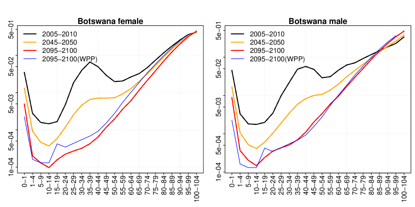
An example of the resulting projected median age-specific mortality rates for Botswana, a country with a generalized HIV/AIDS epidemic, is shown in Figure 8.

Figure 8: Projected age-specific mortality rates for Botswana, a country with a generalized HIV/AIDS epidemic.

There has been recent progress in the modelling of age patterns of mortality for countries with generalized HIV/AIDS (Sharrow et al., 2014). This could provide additional options to better incorporate the uncertainty about future HIV prevalence, expanded access to treatment, underlying age mortality patterns, and their interaction on overall mortality by age into probabilistic population projections. Further calibration and validation of these models using empirical estimates from cohort studies (Zaba et al., 2007; Reniers et al., 2014) will be important in this context.

3 Age-Specific Fertility Rates for Probabilistic Population Projections

3.1 WPP 2012 Method of Projecting Age-Specific Fertility Rates

The United Nations probabilistic population projections released in 2014 (Gerland et al., 2014) used a set of projected age-specific fertility rates for each country obtained by combining probabilistic projections of the total fertility rate with deterministic projections of age patterns of fertility as used in the 2012 revision of the World Population Prospects (United Nations, 2014).

For high-fertility and medium-fertility countries, future age patterns of fertility were obtained by interpolating linearly between a starting proportionate age pattern of fertility and a target model pattern. The target model pattern was chosen from among 15 proportionate age patterns of fertility, with mean age at childbearing varying between 24 and 28.5 years. The target pattern was held constant once the country reaches its lowest fertility level, or by 2045-2050 onward.

For low fertility countries, a similar approach was used. This projected future age-specific fertility patterns by assuming that they would reach a target model pattern by 2025-2030. This target was chosen from among five target age patterns of fertility either for the market economies of Europe (with mean age of childbearing varying between 28 and 32 years) or for countries with economies in transition (with mean age of childbearing varying between 26 and 30 years). Once the model pattern was reached, it was assumed to remain constant until the end of the projection period. In some instances, a modified Lee-Carter approach (Li & Gerland, 2009) was used to extrapolate the most recent set of proportionate age-specific fertility rates using the rates of change from country-specific historical trends.

All the trajectories making up the probabilistic projection of fertility for a given country used the same age pattern of fertility. The choice of target pattern of fertility for a given country, from among the set of model patterns considered, was driven by country-specific expert opinion about future trends and normative assumptions. No global or regional convergence in age patterns of fertility was imposed.

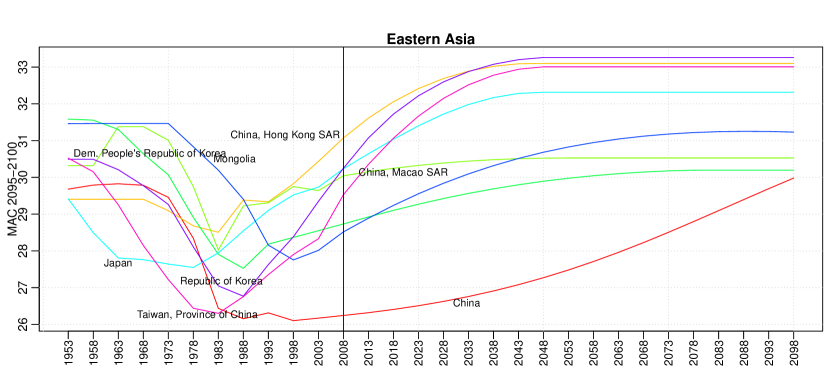
Figure 9 shows the results of the projections for the Mean Age of Childbearing (MAC) for countries in Eastern Asia from the 2012 Revision of the World Population Prospects.

Figure 9: Example of projected Mean Age of Childbearing (MAC) for countries in Eastern Asia in WPP 2012.

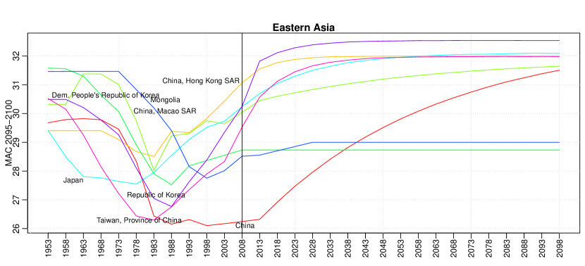
Overall, the method for projecting age-specific patterns of fertility in the 2012 Revision (as well as in previous revisions) has several limitations. First, no global or regional convergence has been imposed despite the overall convergence in total fertility rates observed in the projection period up to 2100. Second, the time point when the target age-specific pattern is reached is not related to the projected total fertility rates. Third, expert assumptions on the target age pattern and method used for individual countries introduce diversity in the age-specific trends are difficult to explain (see Figure 9 — Mongolia and Democratic People’s Republic of Korea were done by Analyst 1, all other countries by Analyst 2). Finally, since the analysts have used at least two different methods and 25 target age patterns of fertility, the documentation of the decisions made for individual countries have been challenging.

3.2 Convergence Method for Projecting Age-Specific Fertility Rates

We now propose a new method for projecting age-specific fertility rates, to overcome some of the limitations of the existing method used in WPP 2012. This builds on the approach adopted in sets of projections of married or in-union women of reproductive age (MWRA) (United Nations, 2013b). Beginning from the most recent observation of the age pattern of fertility in the base period of projection, the projected age patterns of fertility are based on the past national trend combined with the trend towards the global model age pattern of fertility. The projection method is implemented on the proportionate age-specific fertility rates (PASFR) covering seven age groups from 15-19 to 45-49. The final projection of PASFRs for each age group is a weighted average of two preliminary projections:

1. the first preliminary projection, assuming that the PASFRs converge to the global model pattern, see Section 3.2.1; and

2. the second preliminary projection, assuming the observed national trend in PASFRs continues into the indefinite future, see Section 3.2.2.

The method is applied to all the trajectories that make up of the probabilistic projection of total fertility rate for all countries, based on the historical data in the WPP 2012 Revision (Gerland et al., 2014).

We now define the preliminary projections that constitute our overall projection. We use different notation than in Section 2, so the same symbol may be used to denote different quantities in the two sections.

3.2.1 Trend towards the global model pattern

Let $t_{r}$ denote the base period of a projection and $t_{g}$ the year when the global model pattern is reached. For $t_{r}<t<t_{g}$, the proportion of the interval $[t_{r},t_{g}]$ that has elapsed at time $t$ is

$$\tau_{t}=(t-t_{r})/(t_{g}-t_{r}).$$

Section 3.2.4 below gives details about how to estimate $t_{g}$.

Let $p_{r}$ denote PASFR at the base period $t_{r}$, and let $p_{g}$ denote PASFR of the global model pattern. The projections at time $t$ of PASFR towards the global model pattern, denoted by $p_{t}^{I}$, is obtained by:

$$\text{logit}(p_{t}^{I}) = \text{logit}(p_{r})+\tau_{t}\left[\text{logit}(p_{g})-\text{logit}(p_{r})\right]$$ (19)

Then $p_{t}^{I}$ is renormalized so that it sums to unity for all time periods $t$.

3.2.2 Continuing of observed national trend

Let $T$ denote the number of 5-year periods over which the model is fitted. Then $t_{r-T}$ is the starting time period of the estimation and $p_{(r-T)}$ is PASFR at $t_{r-T}$. $p_{t}^{II}$ is the projected PASFR at time $t$, assuming the past trend was to continue into the future under the following rule:

$$\text{logit}(p_{t}^{II}) = \text{logit}(p_{r})+\dfrac{t-t_{r}}{t_{r}-t_{r-T}}\left[\text{logit}(p_{r})-\text{logit}(p_{r-T})\right]$$ (20)

As above, $p_{t}^{II}$ should be scaled to sum to unity for all $t$. Note that in our implementation we use $T=3$.

3.2.3 Resulting projection

Projected PASFR at time $t$, $p_{t}$, is calculated as:

$$\text{logit}(p_{t}) = \tau_{t}\cdot{\text{logit}}(p_{t}^{I})+(1-\tau_{t})\text{ logit}(p_{t}^{II})$$ (21)

Resulting $p_{t}$ is renormalized to sums to unity for all time periods $t$.

3.2.4 Estimating the time period of reaching global pattern

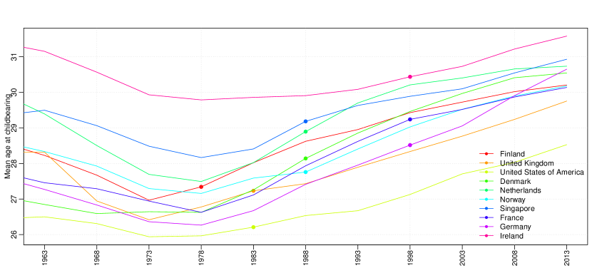
We assume that the transition from the most recent age pattern of fertility to the global model age pattern of fertility is dependent on the timing when the total fertility rate (TFR) enters Phase III, i.e. when the fertility transition is completed and the country reaches low fertility. For the countries in Phase III, a time series model to project TFR was used that assumed that in the long run fertility would approach and fluctuate around country-specific ultimate fertility levels based on a Bayesian hierarchical model (Raftery et al., 2014). The time series model uses the empirical evidence from low-fertility countries that have experienced fertility increases from a sub-replacement level after a completed fertility transition. At the same time, based on the empirical evidence on the postponement of childbearing in low-fertility countries, profound shifts to later start of childbearing and an increase in the mean age of childbearing are still taking place several periods after the start of Phase III (see Figure 10). The timing and speed of the postponement of childbearing in Phase III is country-specific and in this paper we implement the assumption that the transition to later childbearing pattern is completed when total fertility approaches country-specific ultimate fertility levels.

Figure 10: Trends in Mean Age at Childbearing in countries with the start of Phase III of fertility decline before 2000. Dots mark the time period when the country entered Phase III.

To be more specific, we assume that the time $t_{g}$ of a completion of the transition to a global model pattern corresponds to the time point $t_{u}$, when TFR reaches the ultimate fertility level of that country. In probabilistic projections of TFR, we approximate the ultimate fertility level, denoted by $f_{u}$, by the median TFR in the last projection period $t_{e}$, e.g. $t_{e}=$ 2095-2100, if TFR is in Phase III:

$$\hat{f}_{u} = \text{median}_{i}\left[f_{i}(t_{e})\right]\quad(i\text{ denotes trajectories})$$ (22)

Then for each TFR trajectory, $t_{u}$ is the earliest time period, at which the TFR is larger or equal to $\hat{f}_{u}$:

$$t_{u} = \min\{t:f(t)\geqslant\hat{f}_{u}\;\text{ and }\;t>t_{P3}\}$$ (23)

where $t_{P3}$ denotes the start of Phase III. For the estimation of $t_{g}$, we will now distinguish two cases, depending if $t_{P3}$ is smaller or larger than the end period $t_{e}$.

Case 1: $t_{P3}<t_{e}$

In this case, $t_{P3}$ is either observed ($t_{P3}\leqslant t_{r}$) or projected within the projecting period ($t_{r}<t_{P3}<t_{e}$). In both cases, if $t_{u}$ exists,

$$t_{g} = \max(t_{u},t_{r}+10)\,.$$ (24)

This includes a situation where $f(t)\geqslant\hat{f}_{u}$ for $t\leqslant t_{r}$. In such a case, the global pattern is reached quickly, namely in two 5-year periods.

If $f(t)<\hat{f}_{u}$ for all $t_{r}\leqslant t\leqslant t_{e}$, then $t_{u}$ does not exist. In such a case, $t_{g}$ is set to the end of the projection period, but at least five 5-year periods after $t_{P3}$:

$$t_{g} = \max(t_{e},t_{P3}+25)$$ (25)

Case 2: $t_{e}\leqslant t_{P3}$

In this case, $t_{P3}$ is unknown, i.e. the TFR trajectory has not reached Phase III at $t_{e}$. Thus, we will make an estimate of $t_{P3}$, denoted by $\hat{t}_{P3}$, and then simply apply

$$t_{g} = \hat{t}_{P3}+25\,.$$ (26)

If the TFR at $t_{e}$ is low, namely $f(t_{e})\leqslant 1.8$, we assume that $\hat{t}_{P3}=t_{e}$. Otherwise, we approximate $t_{P3}$ by a linear extrapolation of TFR from the last four time periods and determine when such line reaches 1.8, with an upper limit of $\hat{t}_{P3}=t_{e}+50$.

3.2.5 Exception for late childbearing pattern

Since trajectories for some countries have already observed or – as projected by the algorithm described above – will in near future reach higher MAC than the MAC associated with the global model pattern, we assume that for a given country’s trajectory once the maximum MAC is reached in the convergence period the associated PASFR pattern is kept constant for the remaining projection periods. This assumption enables to keep trajectory-specific patterns of late childbearing for trajectories after the Phase III, thus already with low total fertility (see Figure 11 for example of the Czech Republic). Note that this rule is applied only in Case 1 above.

3.3 Results of the convergence method applied to probabilistic projections

For the 2012 Revision, age-specific fertility estimates are based on empirical data for all countries of the world for the period up to 2010 (or up to 2010-2015 for 37 countries with empirical data up to 2011 or 2012; Gerland et al., 2014). Using the probabilistic projections of TFR, each TFR trajectory has a specific start of Phase III and therefore the timing of convergence to the global model pattern is trajectory-specific. This yields a set of trajectories of PASFR (although not probabilistic) which in turn, when combined with the probabilistic TFR, yield probabilistic projection of age-specific fertility rates.

Figure 11 shows an example of the results for PASFR in Niger, Bangladesh and Czech Republic for selected age groups over time. Figure 12 shows an example of the probabilistic results of age-specific fertility rates for Ethiopia, Nepal and Japan at the end of projection period in 2095-2100.

Figure 11: Proportionate age-specific fertility rates (PASFR) by time for age groups 15-19, 25-29 and 35-39 in Niger, Bangladesh and the Czech Republic. Projected median of PASFR (red line) approaches global model pattern of PASFR (black dashed line). The solid grey lines are trajectories that correspond to different starting periods for Phase III; they do not represent random samples from a predictive probability distribution.

Figure 12: Probabilistic projection of age-specific fertility rates for Ethiopia (left panel), Nepal (middle panel) and Japan (right panel) in the time period 2095-2100. The marginal distribution for age-specific fertility rates (red lines) where the dashed lines mark the 80% probability intervals and the solid grey lines are randomly sampled trajectories are compared to age-specific fertility rates in the time period 2005-2010 (blue line) and to the global model pattern applied to median projection of total fertility for the world in 2095-2100 (black dashed line).

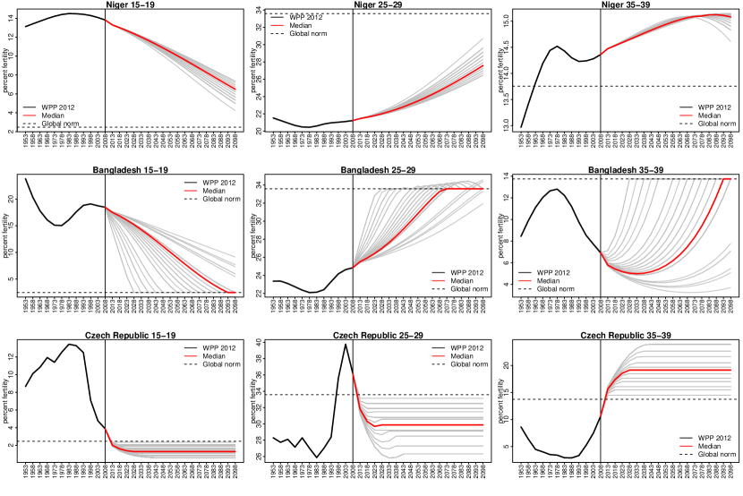
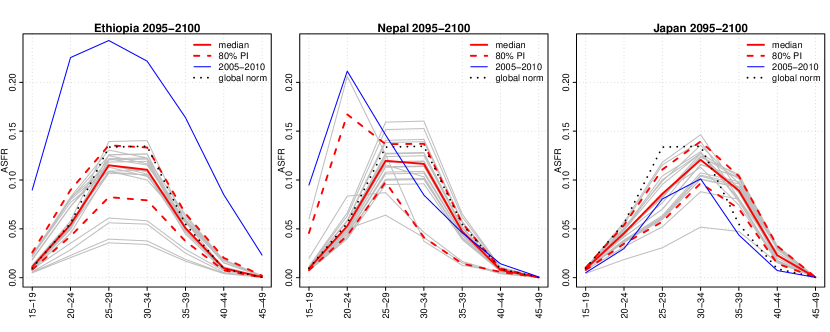
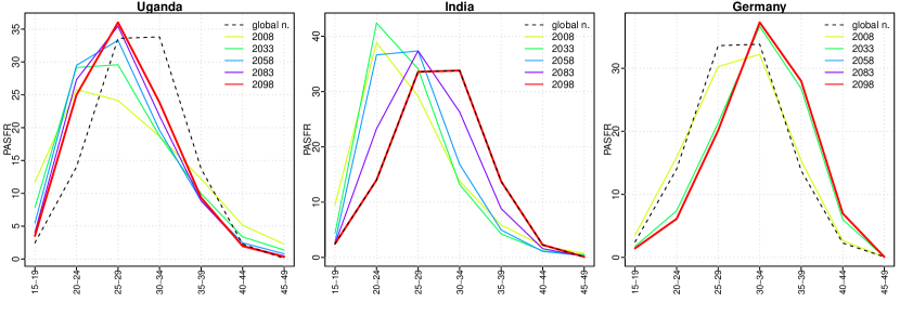
Figure 13 shows the development of PASFR for Uganda, India and Germany over time from 2005-2010 to 2095-2100. Here, the methodology was applied to the deterministic projection of TFR from WPP 2012.

Figure 13: PASFR by age over time for selected countries.

In Figure 9 we showed projections of MAC from WPP 2012. This can be compared to Figure 14 where the same measure is shown after applying the new methodology to the TFR of WPP 2012.

Figure 14: Example of projected MAC for countries in Eastern Asia after applying the proposed methodology.

Overall, the new method we propose improves on the current methodology in several ways. First, in the very long term (after 2100) the age patterns of fertility are converging to one global pattern, while retaining specific late childbearing patterns for several countries that reach such patterns in the current period or in the near future. Second, the projections of the age pattern of fertility are now linked to projections of the total fertility rate. Finally, for each probabilistic trajectory, the time when the target age pattern is reached depends on the trajectory-specific total fertility rate.

4 Discussion

We have described the methods used for converting projected life expectancies at birth and total fertility rates to age-specific mortality and fertility rates in the UN’s 2014 probabilistic population projections. We have identified some limitations of these methods and have proposed several improvements to overcome them. These include a new coherent Kannisto method to avoid crossovers in mortality rates between the sexes at very high ages. They also include the application of a coherent Lee-Carter method, methods for avoiding jump-off bias, and a rotated Lee-Carter method to reflect the fact that at high life expectancies, mortality rates tend to decline faster at higher than at lower ages.

It should be noted that the 2014 PPP takes account of uncertainty about the overall level of fertility as measured by the TFR, and also about the overall level of mortality as measured by $e_{0}$. Conditional on TFR and $e_{0}$, however, the projected vital rates are deterministic. There is thus a missing component of uncertainty, and it would be desirable to extend the methods used to take account of this, particularly of uncertainty about the future mean age at childbearing (Ediev, 2013).

5 Acknowledgements

This research was supported by NIH grants R01 HD054511 and R01 HD070936. The views expressed in this article are those of the authors and do not necessarily reflect those of NIH or the United Nations.

References

- Alkema et al. (2011) Alkema, L., Raftery, A. E., Gerland, P., Clark, S. J., Pelletier, F., Buettner, T., & Heilig, G. K. (2011). Probabilistic projections of the total fertility rate for all countries. Demography, 48, 815–839.
- Booth et al. (2006) Booth, H., Hyndman, R. J., Tickle, L., & de Jong, P. (2006). Lee-Carter mortality forecasting: A multi-country comparison of variants and extensions. Demographic Research, 15.
- Coale & Demeny (1966) Coale, A. J. & Demeny, P. G. (1966). Regional Model Life Tables and Stable Populations. Princeton, N.J.,: Princeton University Press.
- Ediev (2013) Ediev, D. M. (2013). Comparative importance of the fertility model, the total fertility, the mean age and the standard deviation of age at childbearing in population projections. Presented at the Meeting of the International Union for the Scientific Study of Population, Busan, Korea. http://iussp.org/sites/default/files/event_call_for_papers/TF%20MS%20SD_what%20matters_StWr.pdf.
- Gerland et al. (2014) Gerland, P., Raftery, A. E., Ševčíková, H., Li, N., Gu, D., Spoorenberg, T., Alkema, L., Fosdick, B. K., Chunn, J. L., Lalic, N., Bay, G., Buettner, T., Heilig, G. K., & Wilmoth, J. (2014). World population stabilization unlikely this century. Science, 346, 234–237.
- Greville (1943) Greville, T. N. (1943). Short methods of constructing abridged life tables. The Record of the American Institute of Actuaries, XXXII, part 1, 29–42.
- Lee & Carter (1992) Lee, R. D. & Carter, L. (1992). Modeling and forecasting the time series of US mortality. Journal of the American Statistical Association, 87, 659–671.
- Lee & Miller (2001) Lee, R. D. & Miller, T. (2001). Evaluating the performance of the Lee-Carter method for forecasting mortality. Demography, 38, 537–549.
- Li & Gerland (2009) Li, N. & Gerland, P. (2009). Modelling and projecting the postponement of childbearing in low-fertility countries. Presented at theXXVI IUSSP International Population Conference. iussp2009.princeton.edu/papers/90315.
- Li & Gerland (2011) Li, N. & Gerland, P. (2011). Modifying the Lee-Carter method to project mortality changes up to 2100. Presented at the Annual Meeting of Population Association of America. http://paa2011.princeton.edu/abstracts/110555.
- Li & Lee (2005) Li, N. & Lee, R. D. (2005). Coherent mortality forecasts for a group of populations: An extension of the Lee-Carter method. Demography, 42, 575–594.
- Li et al. (2013) Li, N., Lee, R. D., & Gerland, P. (2013). Extending the Lee-Carter method to model the rotation of age patterns of mortality decline for long-term projections. Demography, 50, 2037–2051.
- Raftery et al. (2014) Raftery, A. E., Alkema, L., & Gerland, P. (2014). Bayesian population projections for the United Nations. Statistical Science, 29, 58–68.
- Raftery et al. (2013) Raftery, A. E., Chunn, J. L., Gerland, P., & Ševčíková, H. (2013). Bayesian probabilistic projections of life expectancy for all countries. Demography, 50, 777–801.
- Raftery et al. (2014) Raftery, A. E., Lalic, N., & Gerland, P. (2014). Joint probabilistic projection of female and male life expectancy. Demographic Research, 30, 795–822.
- Raftery et al. (2012) Raftery, A. E., Li, N., Ševčíková, H., Gerland, P., & Heilig, G. K. (2012). Bayesian probabilistic population projections for all countries. Proceedings of the National Academy of Sciences, 109, 13915–13921.
- Reniers et al. (2014) Reniers, G., Slaymaker, E., Nakiyingi-Miiro, J., Nyamukapa, C., Crampin, A. C., Herbst, K., Urassa, M., Otieno, F., Gregson, S., Sewe, M., Michael, D., Lutalo, T., Hosegood, V., Kasamba, I., Price, A., Nabukalu, D., Mclean, E., Zaba, B., & Network”, A. (2014). Mortality trends in the era of antiretroviral therapy: evidence from the Network for Analysing Longitudinal Population based HIV/AIDS data on Africa (ALPHA). AIDS, 28, S533–S542.
- Ševčíková & Raftery (2014) Ševčíková, H. & Raftery, A. (2014). bayesPop: Probabilistic Population Projection. R package version 5.2-2.
- Ševčíková et al. (2014) Ševčíková, H., Raftery, A., & Gerland, P. (2014). Bayesian probabilistic population projections: Do it yourself. Presented at the annual meeting of Population Association of America. http://paa2014.princeton.edu/abstracts/141301.
- Sharrow et al. (2014) Sharrow, D., Clark, S., & Raftery, A. (2014). Modeling age-specific mortality for countries with generalized HIV epidemics. PLoS One, 9.
- Thatcher et al. (1998) Thatcher, A. R., Kannisto, V., & Vaupel, J. W. (1998). The Force of Mortality at Ages 80 to 120, volume 5 of Odense Monographs on Population Aging Series. Odense, Denmark: Odense University Press.
- United Nations (1988) United Nations (1988). MortPak – The United Nations Software Package for Mortality Measurement. Bach-oriented Software for the Mainframe Computer, volume ST/ESA/SER.R/78. New York: United Nations.
- United Nations (2013a) United Nations (2013a). MortPak for Windows Version 4.3 – The United Nations Software Package for Demographic Mortality Measurement.
- United Nations (2013b) United Nations (2013b). National, Regional and Global Estimates and Projections of the Number of Women Aged 15 to 49 Who Are Married or in a Union, 1970-2030, Technical Paper 2013/2. New York, NY: Population Division, Dept. of Economic and Social Affairs, United Nations.
- United Nations (2013c) United Nations (2013c). World Population Prospects: The 2012 Revision - Online and DVD Edition - Data Sources and Meta Information (POP/DB/WPP/Rev.2012/F0-2). New York: Population Division, Dept. of Economic and Social Affairs.
- United Nations (2014) United Nations (2014). World Population Prospects: The 2012 Revision, Methodology of the United Nations Population Estimates and Projections. ESA/P/WP.235. New York, NY: Population Division, Dept. of Economic and Social Affairs, United Nations.
- Wilmoth et al. (2007) Wilmoth, J., Andreev, K., Jdanov, D., & Glei, D. (2007). Methods protocol for the Human Mortality Database. Online publication of the Human Mortality Database. http://www.mortality.org/Public/Docs/MethodsProtocol.pdf.
- Zaba et al. (2007) Zaba, B., Marston, M., Crampin, A. C., Isingo, R., Biraro, S., Barnighausen, T., Lopman, B., Lutalo, T., Glynn, J. R., & Todd, J. (2007). Age-specific mortality patterns in HIV-infected individuals: A comparative analysis of African community study data. Aids, 21 Suppl 6, S87–S96.