Statistical Analysis of Loopy Belief Propagation in Random Fields

Muneki Yasuda Graduate School of Science and Engineering, Yamagata University, Japan.
CREST, JST (Yamagata University)
   Shun Kataoka and Kazuyuki Tanaka Graduate School of Information Sciences, Tohoku University, Japan.
CREST, JST (Tohoku University)
Abstract

Loopy belief propagation (LBP), which is equivalent to the Bethe approximation in statistical mechanics, is a message-passing-type inference method that is widely used to analyze systems based on Markov random fields (MRFs). In this paper, we propose a message-passing-type method to analytically evaluate the quenched average of LBP in random fields by using the replica cluster variation method. The proposed analytical method is applicable to general pair-wise MRFs with random fields whose distributions differ from each other and can give the quenched averages of the Bethe free energies over random fields, which are consistent with numerical results. The order of its computational cost is equivalent to that of standard LBP. In the latter part of this paper, we describe the application of the proposed method to Bayesian image restoration, in which we observed that our theoretical results are in good agreement with the numerical results for natural images.

random field model, loopy belief propagation, replica method, cluster variation method, Bayesian image restoration
pacs:
Valid PACS appear here
preprint: APS/123-QED

I Introduction

Loopy belief propagation (LBP) Pearl (1988), which is a message-passing-type inference method, is widely prevalent in various fields, including computer science, as a powerful tool for statistical procedures in systems based on Markov random fields (MRFs) Opper and Saad (Eds.); Mézard and Montanari (2009). LBP is equivalent to the Bethe approximation in statistical mechanics Kabashima and Saad (1998); Yedidia et al. (2005) and is also known as the cavity method. An analysis of the statistical behaviors of LBP is important to develop an understanding of LBP. In this paper, we focus on LBP in pair-wise MRFs with random fields and we present a statistical analysis of it, namely, an analysis of the quenched average of LBP over random fields. The topic of pair-wise MRFs in random fields is an important research field in statistical mechanics Schneider and Pytte (1977); Krzakala et al. (2010). As described below, a statistical analysis of LBP in random fields is also important for the field of Bayesian signal processing in computer science.

Bayesian image restoration Geman and Geman (1984), in which images degraded by noise are restored using the Bayesian framework, is an important generic technique for various types of signal processing. Suppose that there is an original image and that the original image is degraded through a specific noise process. We observe only the degraded image as the input, and we want to produce the restored image as the output. From the statistical mechanics point of view, the standard framework of Bayesian image restoration corresponds to the framework of a two-dimensional ferromagnetic spin model in random fields Nishimori (2001); Tanaka (2002). In this correspondence, the input image, namely, the degraded image, is regarded as the random fields in the Bayesian image restoration system.

Since the model used in the Bayesian image restoration system is designed by using an intractable pair-wise MRF, LBP is often applied to implement it. Hence, in the evaluation of the statistical performance of the implemented image restoration system, we encounter the evaluation of the quenched average of LBP over the random fields, namely, over the input images. For this purpose, for Ising systems, the authors proposed an analytical evaluation method for it Kataoka et al. (2010); Tanaka et al. (2010). In the previous method, the evaluation of the quenched average of LBP is reduced to solving simultaneous integral equations with respect to the distributions of the messages. However, the method is not very practical, because the computational cost of solving the integral equations is considerable and its approximation accuracy is poor. Furthermore, the method cannot evaluate the quenched average of the free energy and is formulated only in Ising systems.

In this paper, we propose a new analytical method for evaluating the quenched average of LBP over random fields based on the idea of the replica cluster variation method (RCVM) Rizzo et al. (2010); Lage-Castellanos et al. (2013). The presented method allows the quenched average of the Bethe free energies over random fields in general pair-wise MRFs to be evaluated, unlike the previous method.

The remaining part of this paper is organized as follows. A brief explanation of LBP is given in section II. Section III constitutes the main part of the paper. The proposed method is shown in section III.3, and some numerical results for checking its validity are shown in section III.4. In section III.5, we show a case that is exactly solvable by the present method. In section IV, we explain the framework of the framework of Bayesian image restoration and compute the statistical performance of the Bayesian image restoration system using the proposed method. Finally, section V closes the paper with concluding remarks.

II Loopy Belief Propagation in Random Fields

II.1 Model Definition

Let us consider an undirected graph G(V,E)𝐺𝑉𝐸G(V,E) consisting of n𝑛n vertices and some edges, where V={1,2,,n}𝑉12𝑛V=\{1,2,\ldots,n\} is the set of vertices, and E={{i,j}}𝐸𝑖𝑗E=\{\{i,j\}\} is the set of edges between a pair of vertices, where {i,j}𝑖𝑗\{i,j\} denotes the undirected edge between vertices i𝑖i and j𝑗j. On the graph, with the discrete random variables 𝑺{SiiV}𝑺conditional-setsubscript𝑆𝑖𝑖𝑉\bm{S}\in\{S_{i}\mid i\in V\}, let us define the pair-wise MRF expressed by

P(𝑺𝒉,β)𝑃conditional𝑺𝒉𝛽\displaystyle P(\bm{S}\mid\bm{h},\beta) :=1Z(𝒉,β)exp(βH(𝑺;𝒉)),assignabsent1𝑍𝒉𝛽𝛽𝐻𝑺𝒉\displaystyle:=\frac{1}{Z(\bm{h},\beta)}\exp\big{(}-\beta H(\bm{S};\bm{h})\big{)}, (1)

where

H(𝑺;𝒉):=iVϕi(Si,hi){i,j}Eψi,j(Si,Sj)assign𝐻𝑺𝒉subscript𝑖𝑉subscriptitalic-ϕ𝑖subscript𝑆𝑖subscript𝑖subscript𝑖𝑗𝐸subscript𝜓𝑖𝑗subscript𝑆𝑖subscript𝑆𝑗\displaystyle H(\bm{S};\bm{h}):=-\sum_{i\in V}\phi_{i}(S_{i},h_{i})-\sum_{\{i,j\}\in E}\psi_{i,j}(S_{i},S_{j})

is the Hamiltonian of the MRF. Here, ϕi(Si,hi)subscriptitalic-ϕ𝑖subscript𝑆𝑖subscript𝑖\phi_{i}(S_{i},h_{i}) is a specific function of the variable Sisubscript𝑆𝑖S_{i} and the random field hisubscript𝑖h_{i} on vertex i𝑖i, and ϕi,j(Si,Sj)subscriptitalic-ϕ𝑖𝑗subscript𝑆𝑖subscript𝑆𝑗\phi_{i,j}(S_{i},S_{j}) is a specific function on edge {i,j}𝑖𝑗\{i,j\}. The notations, Z𝑍Z and β𝛽\beta, are the partition function and inverse temperature, which takes a positive value, respectively. In this paper, only random fields 𝒉𝒉\bm{h} are treated as the quenched parameters.

II.2 Loopy Belief Propagation

It is known that LBP is derived from the minimum condition of the variational Bethe free energy Yedidia et al. (2005). In this section, we give a brief explanation of the derivation of LBP according to the cluster variation method (CVM) Kikuchi (1951); Pelizzola (2005). The free energy of the MRF in equation (1) is defined by

F(𝒉,β)𝐹𝒉𝛽\displaystyle F(\bm{h},\beta) :=𝑺H(𝑺;𝒉)P(𝑺𝒉,β)assignabsentsubscript𝑺𝐻𝑺𝒉𝑃conditional𝑺𝒉𝛽\displaystyle:=\sum_{\bm{S}}H(\bm{S};\bm{h})P(\bm{S}\mid\bm{h},\beta)
+1β𝑺P(𝑺𝒉,β)lnP(𝑺𝒉,β).1𝛽subscript𝑺𝑃conditional𝑺𝒉𝛽𝑃conditional𝑺𝒉𝛽\displaystyle\quad\>+\frac{1}{\beta}\sum_{\bm{S}}P(\bm{S}\mid\bm{h},\beta)\ln P(\bm{S}\mid\bm{h},\beta). (2)

In the Bethe approximation in the CVM, we approximate the MRF by

P(𝑺𝒉,β)(iVbi(Si))({i,j}Ebi,j(Si,Sj)){i,j}Ebi(Si)bj(Sj),𝑃conditional𝑺𝒉𝛽subscriptproduct𝑖𝑉subscript𝑏𝑖subscript𝑆𝑖subscriptproduct𝑖𝑗𝐸subscript𝑏𝑖𝑗subscript𝑆𝑖subscript𝑆𝑗subscriptproduct𝑖𝑗𝐸subscript𝑏𝑖subscript𝑆𝑖subscript𝑏𝑗subscript𝑆𝑗\displaystyle P(\bm{S}\mid\bm{h},\beta)\approx\frac{\big{(}\prod_{i\in V}b_{i}(S_{i})\big{)}\big{(}\prod_{\{i,j\}\in E}b_{i,j}(S_{i},S_{j})\big{)}}{\prod_{\{i,j\}\in E}b_{i}(S_{i})b_{j}(S_{j})}, (3)

where bi(Si)subscript𝑏𝑖subscript𝑆𝑖b_{i}(S_{i}) and bi,j(Si,Sj)subscript𝑏𝑖𝑗subscript𝑆𝑖subscript𝑆𝑗b_{i,j}(S_{i},S_{j}) are the one-vertex and two-vertex marginal distributions (or the beliefs) of the MRF. This approximation corresponds to the cluster decomposition shown in figure 1. The right-hand side of equation (3) is the product of the marginal distributions of the clusters divided by the product of the marginal distributions of the double-counted clusters. By applying this approximation to P(𝑺𝒉)𝑃conditional𝑺𝒉P(\bm{S}\mid\bm{h}) in the logarithmic function of the last term in equation (2), we obtain the variational Bethe free energy expressed by

bethe[{bi,bi,j}]subscriptbethedelimited-[]subscript𝑏𝑖subscript𝑏𝑖𝑗\displaystyle\mathcal{F}_{\mathrm{bethe}}[\{b_{i},b_{i,j}\}] :=𝑺H(𝑺;𝒉)P(𝑺𝒉,β)+1β𝑺P(𝑺𝒉,β)ln(iVbi(Si))({i,j}Ebi,j(Si,Sj)){i,j}Ebi(Si)bj(Sj)assignabsentsubscript𝑺𝐻𝑺𝒉𝑃conditional𝑺𝒉𝛽1𝛽subscript𝑺𝑃conditional𝑺𝒉𝛽subscriptproduct𝑖𝑉subscript𝑏𝑖subscript𝑆𝑖subscriptproduct𝑖𝑗𝐸subscript𝑏𝑖𝑗subscript𝑆𝑖subscript𝑆𝑗subscriptproduct𝑖𝑗𝐸subscript𝑏𝑖subscript𝑆𝑖subscript𝑏𝑗subscript𝑆𝑗\displaystyle:=\sum_{\bm{S}}H(\bm{S};\bm{h})P(\bm{S}\mid\bm{h},\beta)+\frac{1}{\beta}\sum_{\bm{S}}P(\bm{S}\mid\bm{h},\beta)\ln\frac{\big{(}\prod_{i\in V}b_{i}(S_{i})\big{)}\big{(}\prod_{\{i,j\}\in E}b_{i,j}(S_{i},S_{j})\big{)}}{\prod_{\{i,j\}\in E}b_{i}(S_{i})b_{j}(S_{j})}
=iVSiϕi(Si,hi)bi(Si){i,j}ESi,Sjψi,j(Si,Sj)bi,j(Si,Sj)+1βiV1[bi]absentsubscript𝑖𝑉subscriptsubscript𝑆𝑖subscriptitalic-ϕ𝑖subscript𝑆𝑖subscript𝑖subscript𝑏𝑖subscript𝑆𝑖subscript𝑖𝑗𝐸subscriptsubscript𝑆𝑖subscript𝑆𝑗subscript𝜓𝑖𝑗subscript𝑆𝑖subscript𝑆𝑗subscript𝑏𝑖𝑗subscript𝑆𝑖subscript𝑆𝑗1𝛽subscript𝑖𝑉subscript1delimited-[]subscript𝑏𝑖\displaystyle\>=-\sum_{i\in V}\sum_{S_{i}}\phi_{i}(S_{i},h_{i})b_{i}(S_{i})-\sum_{\{i,j\}\in E}\sum_{S_{i},S_{j}}\psi_{i,j}(S_{i},S_{j})b_{i,j}(S_{i},S_{j})+\frac{1}{\beta}\sum_{i\in V}\mathcal{H}_{1}[b_{i}]
+1β{i,j}E(2[bi,j]1[bi]1[bj]),1𝛽subscript𝑖𝑗𝐸subscript2delimited-[]subscript𝑏𝑖𝑗subscript1delimited-[]subscript𝑏𝑖subscript1delimited-[]subscript𝑏𝑗\displaystyle\quad\>\,+\frac{1}{\beta}\sum_{\{i,j\}\in E}\big{(}\mathcal{H}_{2}[b_{i,j}]-\mathcal{H}_{1}[b_{i}]-\mathcal{H}_{1}[b_{j}]\big{)}, (4)

where

1[bi]:=Sibi(Si)lnbi(Si)assignsubscript1delimited-[]subscript𝑏𝑖subscriptsubscript𝑆𝑖subscript𝑏𝑖subscript𝑆𝑖subscript𝑏𝑖subscript𝑆𝑖\displaystyle\mathcal{H}_{1}[b_{i}]:=\sum_{S_{i}}b_{i}(S_{i})\ln b_{i}(S_{i})

and

2[bi,j]:=Si,Sjbi,j(Si,Sj)lnbi,j(Si,Sj)assignsubscript2delimited-[]subscript𝑏𝑖𝑗subscriptsubscript𝑆𝑖subscript𝑆𝑗subscript𝑏𝑖𝑗subscript𝑆𝑖subscript𝑆𝑗subscript𝑏𝑖𝑗subscript𝑆𝑖subscript𝑆𝑗\displaystyle\mathcal{H}_{2}[b_{i,j}]:=\sum_{S_{i},S_{j}}b_{i,j}(S_{i},S_{j})\ln b_{i,j}(S_{i},S_{j})

are the one-vertex and two-vertex negative entropies.

Refer to caption
Figure 1: (a) Square graph with four vertices. (b) Cluster decomposition of the Bethe approximation of the CVM for (a). The vertices and two connected vertices are selected as the clusters.

LBP is obtained by the variational minimization of the variational Bethe free energy with respect to the beliefs. By minimizing the variational Bethe free energy under the normalizing constraints, Sibi(Si)=Si,Sjbi,j(Si,Sj)=1subscriptsubscript𝑆𝑖subscript𝑏𝑖subscript𝑆𝑖subscriptsubscript𝑆𝑖subscript𝑆𝑗subscript𝑏𝑖𝑗subscript𝑆𝑖subscript𝑆𝑗1\sum_{S_{i}}b_{i}(S_{i})=\sum_{S_{i},S_{j}}b_{i,j}(S_{i},S_{j})=1, and the marginalizing constraints, bi(Si)=Sjbi,j(Si,Sj)subscript𝑏𝑖subscript𝑆𝑖subscriptsubscript𝑆𝑗subscript𝑏𝑖𝑗subscript𝑆𝑖subscript𝑆𝑗b_{i}(S_{i})=\sum_{S_{j}}b_{i,j}(S_{i},S_{j}) and bj(Sj)=Sibi,j(Si,Sj)subscript𝑏𝑗subscript𝑆𝑗subscriptsubscript𝑆𝑖subscript𝑏𝑖𝑗subscript𝑆𝑖subscript𝑆𝑗b_{j}(S_{j})=\sum_{S_{i}}b_{i,j}(S_{i},S_{j}), we obtain the message-passing equation of LBP:

Mij(Sj)subscript𝑀𝑖𝑗subscript𝑆𝑗\displaystyle M_{i\to j}(S_{j}) Siexpβ(ϕi(Si,hi)+ψi,j(Si,Sj))proportional-toabsentsubscriptsubscript𝑆𝑖𝛽subscriptitalic-ϕ𝑖subscript𝑆𝑖subscript𝑖subscript𝜓𝑖𝑗subscript𝑆𝑖subscript𝑆𝑗\displaystyle\propto\sum_{S_{i}}\exp\beta\big{(}\phi_{i}(S_{i},h_{i})+\psi_{i,j}(S_{i},S_{j})\big{)}
×ki{j}Mki(Si),\displaystyle\quad\>\times\prod_{k\in\partial i\setminus\{j\}}M_{k\to i}(S_{i}), (5)

where Mij(Si)subscript𝑀𝑖𝑗subscript𝑆𝑖M_{i\to j}(S_{i}) is the message (or the effective field) from vertex i𝑖i to vertex j𝑗j. Using the messages satisfying the message-passing equation, we can compute the beliefs that minimize the variational Bethe free energy as

bi(Si)subscript𝑏𝑖subscript𝑆𝑖\displaystyle b_{i}(S_{i}) exp(βϕi(Si,hi))jiMji(Si),proportional-toabsent𝛽subscriptitalic-ϕ𝑖subscript𝑆𝑖subscript𝑖subscriptproduct𝑗𝑖subscript𝑀𝑗𝑖subscript𝑆𝑖\displaystyle\propto\exp\big{(}\beta\phi_{i}(S_{i},h_{i})\big{)}\prod_{j\in\partial i}M_{j\to i}(S_{i}), (6)
bi,j(Si,Sj)expβ(ϕi(Si,hi)+ϕj(Sj,hj)\displaystyle b_{i,j}(S_{i},S_{j})\propto\exp\beta\big{(}\phi_{i}(S_{i},h_{i})+\phi_{j}(S_{j},h_{j})
+ψi,j(Si,Sj))ki{j}Mki(Si)lj{i}Mlj(Sj),\displaystyle+\psi_{i,j}(S_{i},S_{j})\big{)}\prod_{k\in\partial i\setminus\{j\}}M_{k\to i}(S_{i})\prod_{l\in\partial j\setminus\{i\}}M_{l\to j}(S_{j}), (7)

where i𝑖\partial i is the set of vertices connected to vertex i𝑖i: i={jjV,{i,j}E}𝑖conditional-set𝑗formulae-sequence𝑗𝑉𝑖𝑗𝐸\partial i=\{j\mid j\in V,\,\{i,j\}\in E\}. The Bethe free energy of the MRF is the minimum of the variational Bethe free energy,

Fbethe(𝒉,β):=min{bi,bij}bethe[{bi,bi,j}],assignsubscript𝐹bethe𝒉𝛽subscriptsubscript𝑏𝑖subscript𝑏𝑖𝑗subscriptbethedelimited-[]subscript𝑏𝑖subscript𝑏𝑖𝑗\displaystyle F_{\mathrm{bethe}}(\bm{h},\beta):=\min_{\{b_{i},b_{ij}\}}\mathcal{F}_{\mathrm{bethe}}[\{b_{i},b_{i,j}\}],

and is obtained by substituting the beliefs obtained by equations (6) and (7) into the variational Bethe free energy in equation (4). In LBP, the beliefs obtained by equations (6) and (7) are regarded as the Bethe approximations of the true marginal distributions of the MRF. When an undirected graph G(V,E)𝐺𝑉𝐸G(V,E), on which the MRF is defined, has no loops, the Bethe free energy and the beliefs are equivalent to the true free energy and the true marginal distributions of the MRF, respectively.

The main proposal presented in this paper is a method for evaluating the quenched average of the Bethe free energy over the random fields:

[Fbethe(𝒉,β)]𝒉:=d𝒉(iVpi(hi))Fbethe(𝒉,β),assignsubscriptdelimited-[]subscript𝐹bethe𝒉𝛽𝒉differential-d𝒉subscriptproduct𝑖𝑉subscript𝑝𝑖subscript𝑖subscript𝐹bethe𝒉𝛽\displaystyle[F_{\mathrm{bethe}}(\bm{h},\beta)]_{\bm{h}}:=\int\mathrm{d}\bm{h}\Big{(}\prod_{i\in V}p_{i}(h_{i})\Big{)}F_{\mathrm{bethe}}(\bm{h},\beta), (8)

where the notation []𝒉subscriptdelimited-[]𝒉[\cdots]_{\bm{h}} represents the average value over the random fields, and pi(hi)subscript𝑝𝑖subscript𝑖p_{i}(h_{i}) is the distribution of the field on vertex i𝑖i, where these distributions can vary by vertex in general.

III Proposed Method

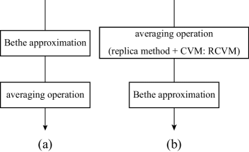
According to equation (8), in principle, we have to perform the averaging operation after constructing the Bethe free energy to obtain [Fbethe]𝒉subscriptdelimited-[]subscript𝐹bethe𝒉[F_{\mathrm{bethe}}]_{\bm{h}} (see figure 2(a)). However, it is not straightforward to directly integrate the Bethe free energy. Thus, we adopt another strategy.

In this paper, we propose an approximate method based on the idea of the RCVM Rizzo et al. (2010); Lage-Castellanos et al. (2013). Figure 2(b) shows the procedure of our method.
Refer to caption
Figure 2: Procedures of obtaining the quenched average of the Bethe free energy. (a) Principled procedure. (b) Procedure of the proposed method based on the RCVM.

In the method, we first take the average of the free energy using the replica method and CVM, namely, the RCVM (section III.1), and then, we apply the Bethe approximation to the resulting form of the RCVM (section III.2). If the exchange of the order of the two operations, the Bethe approximation and the quenched averaging operation, is allowed, we can expect to obtain a good approximation of the quenched average of the Bethe free energy.

III.1 Replica Cluster Variation Method

First, we obtain the quenched average of the true free energy of the MRF in equation (1), that is,

[F(𝒉,β)]𝒉=1βd𝒉(iVpi(hi))lnZ(𝒉,β).subscriptdelimited-[]𝐹𝒉𝛽𝒉1𝛽differential-d𝒉subscriptproduct𝑖𝑉subscript𝑝𝑖subscript𝑖𝑍𝒉𝛽\displaystyle[F(\bm{h},\beta)]_{\bm{h}}=-\frac{1}{\beta}\int\mathrm{d}\bm{h}\Big{(}\prod_{i\in V}p_{i}(h_{i})\Big{)}\ln Z(\bm{h},\beta).

In the context of the replica method Mezard et al. (1987); Nishimori (2001), we have

[F(𝒉,β)]𝒉=1βlimx0Zx1x,subscriptdelimited-[]𝐹𝒉𝛽𝒉1𝛽subscript𝑥0subscript𝑍𝑥1𝑥\displaystyle[F(\bm{h},\beta)]_{\bm{h}}=-\frac{1}{\beta}\lim_{x\to 0}\frac{Z_{x}-1}{x}, (9)

where

Zx:=d𝒉(iVpi(hi))Z(𝒉,β)x.assignsubscript𝑍𝑥differential-d𝒉subscriptproduct𝑖𝑉subscript𝑝𝑖subscript𝑖𝑍superscript𝒉𝛽𝑥\displaystyle Z_{x}:=\int\mathrm{d}\bm{h}\Big{(}\prod_{i\in V}p_{i}(h_{i})\Big{)}Z(\bm{h},\beta)^{x}.

By assuming that x𝑥x is a natural number, we obtain

Zx=𝒮xexpβ(iVei(𝑺i)+{i,j}Eα=1xψi.j(Siα,Sjα)),subscript𝑍𝑥subscriptsubscript𝒮𝑥𝛽subscript𝑖𝑉subscript𝑒𝑖subscript𝑺𝑖subscript𝑖𝑗𝐸superscriptsubscript𝛼1𝑥subscript𝜓formulae-sequence𝑖𝑗superscriptsubscript𝑆𝑖𝛼superscriptsubscript𝑆𝑗𝛼\displaystyle Z_{x}=\sum_{\mathcal{S}_{x}}\exp\beta\Big{(}\sum_{i\in V}e_{i}(\bm{S}_{i})+\sum_{\{i,j\}\in E}\sum_{\alpha=1}^{x}\psi_{i.j}(S_{i}^{\alpha},S_{j}^{\alpha})\Big{)},

where 𝒮x={SiαiV,α=1,2,,x}subscript𝒮𝑥conditional-setsuperscriptsubscript𝑆𝑖𝛼formulae-sequence𝑖𝑉𝛼12𝑥\mathcal{S}_{x}=\{S_{i}^{\alpha}\mid i\in V,\>\alpha=1,2,\ldots,x\}, 𝑺i={Siαα=1,2,,x}subscript𝑺𝑖conditional-setsuperscriptsubscript𝑆𝑖𝛼𝛼12𝑥\bm{S}_{i}=\{S_{i}^{\alpha}\mid\alpha=1,2,\ldots,x\}, and the function ei(𝑺i)subscript𝑒𝑖subscript𝑺𝑖e_{i}(\bm{S}_{i}) is defined by

ei(𝑺i):=1βlndhpi(h)exp(βα=1xϕi(Siα,h)).assignsubscript𝑒𝑖subscript𝑺𝑖1𝛽differential-dsubscript𝑝𝑖𝛽superscriptsubscript𝛼1𝑥subscriptitalic-ϕ𝑖superscriptsubscript𝑆𝑖𝛼\displaystyle e_{i}(\bm{S}_{i}):=\frac{1}{\beta}\ln\int\mathrm{d}h\,p_{i}(h)\exp\Big{(}\beta\sum_{\alpha=1}^{x}\phi_{i}(S_{i}^{\alpha},h)\Big{)}.

We regard 𝒵xsubscript𝒵𝑥\mathcal{Z}_{x} as the partition of the x𝑥x-replicated system and define the x𝑥x-replicated free energy as

Fxsubscript𝐹𝑥\displaystyle F_{x} :=1βlnZxassignabsent1𝛽subscript𝑍𝑥\displaystyle:=-\frac{1}{\beta}\ln Z_{x}
=iV𝑺iei(𝑺i)Qi(𝑺i)+α=1x𝑺αHint(𝑺α)Qα(𝑺α)absentsubscript𝑖𝑉subscriptsubscript𝑺𝑖subscript𝑒𝑖subscript𝑺𝑖subscript𝑄𝑖subscript𝑺𝑖superscriptsubscript𝛼1𝑥subscriptsuperscript𝑺𝛼subscript𝐻intsuperscript𝑺𝛼superscript𝑄𝛼superscript𝑺𝛼\displaystyle\>=-\sum_{i\in V}\sum_{\bm{S}_{i}}e_{i}(\bm{S}_{i})Q_{i}(\bm{S}_{i})+\sum_{\alpha=1}^{x}\sum_{\bm{S}^{\alpha}}H_{\mathrm{int}}(\bm{S}^{\alpha})Q^{\alpha}(\bm{S}^{\alpha})
+1β𝒮xPx(𝒮x)lnPx(𝒮x),1𝛽subscriptsubscript𝒮𝑥subscript𝑃𝑥subscript𝒮𝑥subscript𝑃𝑥subscript𝒮𝑥\displaystyle\quad\>+\frac{1}{\beta}\sum_{\mathcal{S}_{x}}P_{x}(\mathcal{S}_{x})\ln P_{x}(\mathcal{S}_{x}), (10)

where

Px(𝒮x)subscript𝑃𝑥subscript𝒮𝑥\displaystyle P_{x}(\mathcal{S}_{x}) :=1Zxexpβ(iVei(𝑺i)α=1xHint(𝑺α))assignabsent1subscript𝑍𝑥𝛽subscript𝑖𝑉subscript𝑒𝑖subscript𝑺𝑖superscriptsubscript𝛼1𝑥subscript𝐻intsuperscript𝑺𝛼\displaystyle:=\frac{1}{Z_{x}}\exp\beta\Big{(}\sum_{i\in V}e_{i}(\bm{S}_{i})-\sum_{\alpha=1}^{x}H_{\mathrm{int}}(\bm{S}^{\alpha})\Big{)}

is the Gibbs distribution of the x𝑥x-replicated system, and 𝑺α={SiαiV}superscript𝑺𝛼conditional-setsuperscriptsubscript𝑆𝑖𝛼𝑖𝑉\bm{S}^{\alpha}=\{S_{i}^{\alpha}\mid i\in V\}. The energy function Hint(𝑺)subscript𝐻int𝑺H_{\mathrm{int}}(\bm{S}) is defined by

Hint(𝑺):={i,j}Eψi.j(Si,Sj)assignsubscript𝐻int𝑺subscript𝑖𝑗𝐸subscript𝜓formulae-sequence𝑖𝑗subscript𝑆𝑖subscript𝑆𝑗\displaystyle H_{\mathrm{int}}(\bm{S}):=-\sum_{\{i,j\}\in E}\psi_{i.j}(S_{i},S_{j})

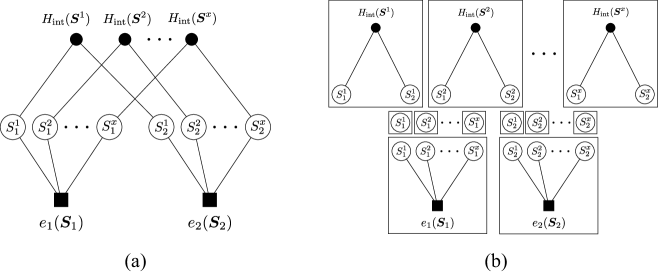
and is just the interaction term of the original system. The distributions, Qi(𝑺i)subscript𝑄𝑖subscript𝑺𝑖Q_{i}(\bm{S}_{i}) and Qα(𝑺α)superscript𝑄𝛼superscript𝑺𝛼Q^{\alpha}(\bm{S}^{\alpha}), are the marginal distributions of the distribution Px(𝒮x)subscript𝑃𝑥subscript𝒮𝑥P_{x}(\mathcal{S}_{x}). The factor graph representation of the x𝑥x-replicated system is shown in figure 3(a).
Refer to caption
Figure 3: (a) Factor graph representation of Px(𝒮x)subscript𝑃𝑥subscript𝒮𝑥P_{x}(\mathcal{S}_{x}) when n=2𝑛2n=2. (b) Cluster decomposition for (a). In the decomposition, the three different types of clusters are employed: the clusters consist of Siαsuperscriptsubscript𝑆𝑖𝛼S_{i}^{\alpha}, of 𝑺isubscript𝑺𝑖\bm{S}_{i}, and of 𝑺αsuperscript𝑺𝛼\bm{S}^{\alpha}.

In accordance with the cluster decomposition based on the CVM shown in figure 3(b), by using the marginal distributions, {Qi(𝑺i),Qα(𝑺α)}subscript𝑄𝑖subscript𝑺𝑖superscript𝑄𝛼superscript𝑺𝛼\{Q_{i}(\bm{S}_{i}),Q^{\alpha}(\bm{S}^{\alpha})\}, together with the one-variable marginal distributions of Px(𝒮x)subscript𝑃𝑥subscript𝒮𝑥P_{x}(\mathcal{S}_{x}), {Qiα(Siα)}superscriptsubscript𝑄𝑖𝛼superscriptsubscript𝑆𝑖𝛼\{Q_{i}^{\alpha}(S_{i}^{\alpha})\}, we approximate the Gibbs distribution of the x𝑥x-replicated system as

Px(𝒮x)(iVα=1xQiα(Siα))(iVQi(𝑺i))(α=1xQα(𝑺α))(iVα=1xQiα(Siα))2=(iVQi(𝑺i))(α=1xQα(𝑺α))iVα=1xQiα(Siα).subscript𝑃𝑥subscript𝒮𝑥subscriptproduct𝑖𝑉superscriptsubscriptproduct𝛼1𝑥superscriptsubscript𝑄𝑖𝛼superscriptsubscript𝑆𝑖𝛼subscriptproduct𝑖𝑉subscript𝑄𝑖subscript𝑺𝑖superscriptsubscriptproduct𝛼1𝑥superscript𝑄𝛼superscript𝑺𝛼superscriptsubscriptproduct𝑖𝑉superscriptsubscriptproduct𝛼1𝑥superscriptsubscript𝑄𝑖𝛼superscriptsubscript𝑆𝑖𝛼2subscriptproduct𝑖𝑉subscript𝑄𝑖subscript𝑺𝑖superscriptsubscriptproduct𝛼1𝑥superscript𝑄𝛼superscript𝑺𝛼subscriptproduct𝑖𝑉superscriptsubscriptproduct𝛼1𝑥superscriptsubscript𝑄𝑖𝛼superscriptsubscript𝑆𝑖𝛼\displaystyle P_{x}(\mathcal{S}_{x})\approx\frac{\big{(}\prod_{i\in V}\prod_{\alpha=1}^{x}Q_{i}^{\alpha}(S_{i}^{\alpha})\big{)}\big{(}\prod_{i\in V}Q_{i}(\bm{S}_{i})\big{)}\big{(}\prod_{\alpha=1}^{x}Q^{\alpha}(\bm{S}^{\alpha})\big{)}}{\big{(}\prod_{i\in V}\prod_{\alpha=1}^{x}Q_{i}^{\alpha}(S_{i}^{\alpha})\big{)}^{2}}=\frac{\big{(}\prod_{i\in V}Q_{i}(\bm{S}_{i})\big{)}\big{(}\prod_{\alpha=1}^{x}Q^{\alpha}(\bm{S}^{\alpha})\big{)}}{\prod_{i\in V}\prod_{\alpha=1}^{x}Q_{i}^{\alpha}(S_{i}^{\alpha})}. (11)

As in equation (3), Px(𝒮x)subscript𝑃𝑥subscript𝒮𝑥P_{x}(\mathcal{S}_{x}) is approximated by the product of the marginal distributions of the clusters divided by the product of the marginal distributions of the double-counted clusters. By applying this approximation to Px(𝒮x)subscript𝑃𝑥subscript𝒮𝑥P_{x}(\mathcal{S}_{x}) in the logarithmic function in the last term in equation (10), we obtain the expression of the variational free energy as

xRCVM[{Qi,Qα,Qiα}]superscriptsubscript𝑥RCVMdelimited-[]subscript𝑄𝑖superscript𝑄𝛼superscriptsubscript𝑄𝑖𝛼\displaystyle\mathcal{F}_{x}^{\mathrm{RCVM}}[\{Q_{i},Q^{\alpha},Q_{i}^{\alpha}\}] :=iV𝒱i[Qi]+α=1x𝒱int[Qα]assignabsentsubscript𝑖𝑉subscript𝒱𝑖delimited-[]subscript𝑄𝑖superscriptsubscript𝛼1𝑥subscript𝒱intdelimited-[]superscript𝑄𝛼\displaystyle:=\sum_{i\in V}\mathcal{V}_{i}[Q_{i}]+\sum_{\alpha=1}^{x}\mathcal{V}_{\mathrm{int}}[Q^{\alpha}]
1βiVα=1x1[Qiα],1𝛽subscript𝑖𝑉superscriptsubscript𝛼1𝑥subscript1delimited-[]superscriptsubscript𝑄𝑖𝛼\displaystyle\quad\>-\frac{1}{\beta}\sum_{i\in V}\sum_{\alpha=1}^{x}\mathcal{H}_{1}[Q_{i}^{\alpha}], (12)

where the functionals, 𝒱i[Qi]subscript𝒱𝑖delimited-[]subscript𝑄𝑖\mathcal{V}_{i}[Q_{i}] and 𝒱int[Qα]subscript𝒱intdelimited-[]superscript𝑄𝛼\mathcal{V}_{\mathrm{int}}[Q^{\alpha}], are defined as

𝒱i[Qi]subscript𝒱𝑖delimited-[]subscript𝑄𝑖\displaystyle\mathcal{V}_{i}[Q_{i}] :=𝑺iei(𝑺i)Qi(𝑺i)+1β𝑺iQi(𝑺i)lnQi(𝑺i),assignabsentsubscriptsubscript𝑺𝑖subscript𝑒𝑖subscript𝑺𝑖subscript𝑄𝑖subscript𝑺𝑖1𝛽subscriptsubscript𝑺𝑖subscript𝑄𝑖subscript𝑺𝑖subscript𝑄𝑖subscript𝑺𝑖\displaystyle:=-\sum_{\bm{S}_{i}}e_{i}(\bm{S}_{i})Q_{i}(\bm{S}_{i})+\frac{1}{\beta}\sum_{\bm{S}_{i}}Q_{i}(\bm{S}_{i})\ln Q_{i}(\bm{S}_{i}), (13)
𝒱int[Qα]subscript𝒱intdelimited-[]superscript𝑄𝛼\displaystyle\mathcal{V}_{\mathrm{int}}[Q^{\alpha}] :=𝑺αHint(𝑺α)Qα(𝑺)+1β𝑺αQα(𝑺α)lnQα(𝑺α).assignabsentsubscriptsuperscript𝑺𝛼subscript𝐻intsuperscript𝑺𝛼superscript𝑄𝛼𝑺1𝛽subscriptsuperscript𝑺𝛼superscript𝑄𝛼superscript𝑺𝛼superscript𝑄𝛼superscript𝑺𝛼\displaystyle:=\sum_{\bm{S}^{\alpha}}H_{\mathrm{int}}(\bm{S}^{\alpha})Q^{\alpha}(\bm{S})+\frac{1}{\beta}\sum_{\bm{S}^{\alpha}}Q^{\alpha}(\bm{S}^{\alpha})\ln Q^{\alpha}(\bm{S}^{\alpha}). (14)

In the context of the CVM, the x𝑥x-replicated free energy in equation (10) is approximated by the minimum of the variational free energy in equation (12) with respect to the marginal distributions {Qi,Qα,Qiα}subscript𝑄𝑖superscript𝑄𝛼superscriptsubscript𝑄𝑖𝛼\{Q_{i},Q^{\alpha},Q_{i}^{\alpha}\}, i.e., Fxmin{Qi,Qα,Qiα}xRCVM[{Qi,Qα,Qiα}]subscript𝐹𝑥subscriptsubscript𝑄𝑖superscript𝑄𝛼superscriptsubscript𝑄𝑖𝛼superscriptsubscript𝑥RCVMdelimited-[]subscript𝑄𝑖superscript𝑄𝛼superscriptsubscript𝑄𝑖𝛼F_{x}\approx\min_{\{Q_{i},Q^{\alpha},Q_{i}^{\alpha}\}}\mathcal{F}_{x}^{\mathrm{RCVM}}[\{Q_{i},Q^{\alpha},Q_{i}^{\alpha}\}]. Note that, at the minimum point, the normalization constraints for {Qi,Qα,Qiα}subscript𝑄𝑖superscript𝑄𝛼superscriptsubscript𝑄𝑖𝛼\{Q_{i},Q^{\alpha},Q_{i}^{\alpha}\} and the marginal constraints,

Qiα(Siα)superscriptsubscript𝑄𝑖𝛼superscriptsubscript𝑆𝑖𝛼\displaystyle Q_{i}^{\alpha}(S_{i}^{\alpha}) =𝑺i{Siα}Qi(𝑺i)absentsubscriptsubscript𝑺𝑖superscriptsubscript𝑆𝑖𝛼subscript𝑄𝑖subscript𝑺𝑖\displaystyle=\sum_{\bm{S}_{i}\setminus\{S_{i}^{\alpha}\}}Q_{i}(\bm{S}_{i}) (15)

and

Qiα(Siα)superscriptsubscript𝑄𝑖𝛼superscriptsubscript𝑆𝑖𝛼\displaystyle Q_{i}^{\alpha}(S_{i}^{\alpha}) =𝑺α{Siα}Qα(𝑺α),absentsubscriptsuperscript𝑺𝛼superscriptsubscript𝑆𝑖𝛼superscript𝑄𝛼superscript𝑺𝛼\displaystyle=\sum_{\bm{S}^{\alpha}\setminus\{S_{i}^{\alpha}\}}Q^{\alpha}(\bm{S}^{\alpha}), (16)

should hold.

In order to minimize the variational free energy with respect to {Qi(𝑺i)}subscript𝑄𝑖subscript𝑺𝑖\{Q_{i}(\bm{S}_{i})\}, by using the Lagrange multipliers, we perform the variational minimization of

[{Qi}]:=iV𝒱i[Qi]iVai(𝑺iQi(𝑺i)1)assigndelimited-[]subscript𝑄𝑖subscript𝑖𝑉subscript𝒱𝑖delimited-[]subscript𝑄𝑖subscript𝑖𝑉subscript𝑎𝑖subscriptsubscript𝑺𝑖subscript𝑄𝑖subscript𝑺𝑖1\displaystyle\mathcal{L}[\{Q_{i}\}]:=\sum_{i\in V}\mathcal{V}_{i}[Q_{i}]-\sum_{i\in V}a_{i}\Big{(}\sum_{\bm{S}_{i}}Q_{i}(\bm{S}_{i})-1\Big{)}
iVα=1xSiαΛiα(Siα)(𝑺i{Siα}Qi(𝑺i)Qiα(Siα))subscript𝑖𝑉superscriptsubscript𝛼1𝑥subscriptsuperscriptsubscript𝑆𝑖𝛼superscriptsubscriptΛ𝑖𝛼superscriptsubscript𝑆𝑖𝛼subscriptsubscript𝑺𝑖superscriptsubscript𝑆𝑖𝛼subscript𝑄𝑖subscript𝑺𝑖superscriptsubscript𝑄𝑖𝛼superscriptsubscript𝑆𝑖𝛼\displaystyle-\sum_{i\in V}\sum_{\alpha=1}^{x}\sum_{S_{i}^{\alpha}}\Lambda_{i}^{\alpha}(S_{i}^{\alpha})\Big{(}\sum_{\bm{S}_{i}\setminus\{S_{i}^{\alpha}\}}Q_{i}(\bm{S}_{i})-Q_{i}^{\alpha}(S_{i}^{\alpha})\Big{)}

with respect to {Qi(𝑺i)}subscript𝑄𝑖subscript𝑺𝑖\{Q_{i}(\bm{S}_{i})\}. From the result of this minimization, we obtain

Qi(𝑺i)expβ(ei(𝑺i)+α=1xΛiα(Siα)).proportional-tosubscript𝑄𝑖subscript𝑺𝑖𝛽subscript𝑒𝑖subscript𝑺𝑖superscriptsubscript𝛼1𝑥superscriptsubscriptΛ𝑖𝛼superscriptsubscript𝑆𝑖𝛼\displaystyle Q_{i}(\bm{S}_{i})\propto\exp\beta\Big{(}e_{i}(\bm{S}_{i})+\sum_{\alpha=1}^{x}\Lambda_{i}^{\alpha}(S_{i}^{\alpha})\Big{)}. (17)

The Lagrange multipliers, 𝚲i={Λiα(Si)α=1,2,,x}subscript𝚲𝑖conditional-setsuperscriptsubscriptΛ𝑖𝛼subscript𝑆𝑖𝛼12𝑥\bm{\Lambda}_{i}=\{\Lambda_{i}^{\alpha}(S_{i})\mid\alpha=1,2,\ldots,x\}, are determined such that they satisfy equation (15). By substituting equation (17) into equation (13), while noting the marginal constraints in equation (15), we obtain the partially minimized variational free energy,

xRCVM[{Qα,Qiα}]:=min{Qi}xRCVM[{Qi,Qα,Qiα}],assignsuperscriptsubscript𝑥RCVMdelimited-[]superscript𝑄𝛼superscriptsubscript𝑄𝑖𝛼subscriptsubscript𝑄𝑖superscriptsubscript𝑥RCVMdelimited-[]subscript𝑄𝑖superscript𝑄𝛼superscriptsubscript𝑄𝑖𝛼\displaystyle\mathcal{F}_{x}^{\mathrm{RCVM}}[\{Q^{\alpha},Q_{i}^{\alpha}\}]:=\min_{\{Q_{i}\}}\mathcal{F}_{x}^{\mathrm{RCVM}}[\{Q_{i},Q^{\alpha},Q_{i}^{\alpha}\}],

as

xRCVM[{Qα,Qiα}]=iVextr𝚲i{α=1xSiαΛiα(Siα)Qiα(Siα)\displaystyle\mathcal{F}_{x}^{\mathrm{RCVM}}[\{Q^{\alpha},Q_{i}^{\alpha}\}]=\sum_{i\in V}\underset{\bm{\Lambda}_{i}}{\mathrm{extr}}\Big{\{}\sum_{\alpha=1}^{x}\sum_{S_{i}^{\alpha}}\Lambda_{i}^{\alpha}(S_{i}^{\alpha})Q_{i}^{\alpha}(S_{i}^{\alpha})
1βlndhpi(h)α=1xSiαexpβ(ϕi(Siα,h)\displaystyle-\frac{1}{\beta}\ln\int\mathrm{d}h\,p_{i}(h)\prod_{\alpha=1}^{x}\sum_{S_{i}^{\alpha}}\exp\beta\big{(}\phi_{i}(S_{i}^{\alpha},h)
+Λiα(Siα))}+α=1x𝒱int[Qα]1βiVα=1x1[Qiα],\displaystyle+\Lambda_{i}^{\alpha}(S_{i}^{\alpha})\big{)}\Big{\}}+\sum_{\alpha=1}^{x}\mathcal{V}_{\mathrm{int}}[Q^{\alpha}]-\frac{1}{\beta}\sum_{i\in V}\sum_{\alpha=1}^{x}\mathcal{H}_{1}[Q_{i}^{\alpha}], (18)

where the notation “extr” denotes the extremum with respect to the assigned parameters.

III.2 Bethe Approximation and Replica Symmetric Ansatz

The functional 𝒱int[Qα]subscript𝒱intdelimited-[]superscript𝑄𝛼\mathcal{V}_{\mathrm{int}}[Q^{\alpha}] can be interpreted as the variational free energy for the interaction term of the original system (see equation (14)). Since this variational free energy is intractable in general, we approximate it by the Bethe approximation. As in equation (3), we approximate Qα(𝑺α)superscript𝑄𝛼superscript𝑺𝛼Q^{\alpha}(\bm{S}^{\alpha}) by

Qα(𝑺α)(iVQiα(Siα))({i,j}EQi,jα(Siα,Sjα)){i,j}EQiα(Siα)Qjα(Sjα),superscript𝑄𝛼superscript𝑺𝛼subscriptproduct𝑖𝑉superscriptsubscript𝑄𝑖𝛼superscriptsubscript𝑆𝑖𝛼subscriptproduct𝑖𝑗𝐸superscriptsubscript𝑄𝑖𝑗𝛼superscriptsubscript𝑆𝑖𝛼superscriptsubscript𝑆𝑗𝛼subscriptproduct𝑖𝑗𝐸superscriptsubscript𝑄𝑖𝛼superscriptsubscript𝑆𝑖𝛼superscriptsubscript𝑄𝑗𝛼superscriptsubscript𝑆𝑗𝛼\displaystyle Q^{\alpha}(\bm{S}^{\alpha})\approx\frac{\big{(}\prod_{i\in V}Q_{i}^{\alpha}(S_{i}^{\alpha})\big{)}\big{(}\prod_{\{i,j\}\in E}Q_{i,j}^{\alpha}(S_{i}^{\alpha},S_{j}^{\alpha})\big{)}}{\prod_{\{i,j\}\in E}Q_{i}^{\alpha}(S_{i}^{\alpha})Q_{j}^{\alpha}(S_{j}^{\alpha})}, (19)

where the distributions, Qiα(Siα)superscriptsubscript𝑄𝑖𝛼superscriptsubscript𝑆𝑖𝛼Q_{i}^{\alpha}(S_{i}^{\alpha}) and Qi,jα(Siα,Sjα)superscriptsubscript𝑄𝑖𝑗𝛼superscriptsubscript𝑆𝑖𝛼superscriptsubscript𝑆𝑗𝛼Q_{i,j}^{\alpha}(S_{i}^{\alpha},S_{j}^{\alpha}), are the marginal distributions of Qα(𝑺α)superscript𝑄𝛼superscript𝑺𝛼Q^{\alpha}(\bm{S}^{\alpha}), so that the marginal constraints,

SiαQi,jα(Siα,Sjα)subscriptsuperscriptsubscript𝑆𝑖𝛼superscriptsubscript𝑄𝑖𝑗𝛼superscriptsubscript𝑆𝑖𝛼superscriptsubscript𝑆𝑗𝛼\displaystyle\sum_{S_{i}^{\alpha}}Q_{i,j}^{\alpha}(S_{i}^{\alpha},S_{j}^{\alpha}) =Qjα(Sjα)absentsuperscriptsubscript𝑄𝑗𝛼superscriptsubscript𝑆𝑗𝛼\displaystyle=Q_{j}^{\alpha}(S_{j}^{\alpha})

and

SjαQi,jα(Siα,Sjα)subscriptsuperscriptsubscript𝑆𝑗𝛼superscriptsubscript𝑄𝑖𝑗𝛼superscriptsubscript𝑆𝑖𝛼superscriptsubscript𝑆𝑗𝛼\displaystyle\sum_{S_{j}^{\alpha}}Q_{i,j}^{\alpha}(S_{i}^{\alpha},S_{j}^{\alpha}) =Qiα(Siα),absentsuperscriptsubscript𝑄𝑖𝛼superscriptsubscript𝑆𝑖𝛼\displaystyle=Q_{i}^{\alpha}(S_{i}^{\alpha}),

are satisfied. By applying equation (19) to Qα(𝑺α)superscript𝑄𝛼superscript𝑺𝛼Q^{\alpha}(\bm{S}^{\alpha}) in the logarithmic function in the last term of equation (14), we obtain the Bethe approximation of 𝒱int[Qα]subscript𝒱intdelimited-[]superscript𝑄𝛼\mathcal{V}_{\mathrm{int}}[Q^{\alpha}] as

𝒱intbethe[{Qiα,Qi,jα}]superscriptsubscript𝒱intbethedelimited-[]superscriptsubscript𝑄𝑖𝛼superscriptsubscript𝑄𝑖𝑗𝛼\displaystyle\mathcal{V}_{\mathrm{int}}^{\mathrm{bethe}}[\{Q_{i}^{\alpha},Q_{i,j}^{\alpha}\}]
:={i,j}ESiα,Sjαψi,j(Siα,Sjα)Qi,jα(Siα,Sjα)assignabsentsubscript𝑖𝑗𝐸subscriptsuperscriptsubscript𝑆𝑖𝛼superscriptsubscript𝑆𝑗𝛼subscript𝜓𝑖𝑗superscriptsubscript𝑆𝑖𝛼superscriptsubscript𝑆𝑗𝛼superscriptsubscript𝑄𝑖𝑗𝛼superscriptsubscript𝑆𝑖𝛼superscriptsubscript𝑆𝑗𝛼\displaystyle:=-\sum_{\{i,j\}\in E}\sum_{S_{i}^{\alpha},S_{j}^{\alpha}}\psi_{i,j}(S_{i}^{\alpha},S_{j}^{\alpha})Q_{i,j}^{\alpha}(S_{i}^{\alpha},S_{j}^{\alpha})
+1βiV1[Qiα]+1β{i,j}E(2[Qi,jα]1[Qiα]1[Qjα]).1𝛽subscript𝑖𝑉subscript1delimited-[]superscriptsubscript𝑄𝑖𝛼1𝛽subscript𝑖𝑗𝐸subscript2delimited-[]superscriptsubscript𝑄𝑖𝑗𝛼subscript1delimited-[]superscriptsubscript𝑄𝑖𝛼subscript1delimited-[]superscriptsubscript𝑄𝑗𝛼\displaystyle+\frac{1}{\beta}\sum_{i\in V}\mathcal{H}_{1}[Q_{i}^{\alpha}]+\frac{1}{\beta}\sum_{\{i,j\}\in E}\big{(}\mathcal{H}_{2}[Q_{i,j}^{\alpha}]-\mathcal{H}_{1}[Q_{i}^{\alpha}]-\mathcal{H}_{1}[Q_{j}^{\alpha}]\big{)}. (20)

By substituting the Bethe approximation in equation (20) into equation (18), we obtain the Bethe approximation of equation (18): xRCVM[{Qα,Qiα}]xLBP[{Qiα,Qi,jα}]superscriptsubscript𝑥RCVMdelimited-[]superscript𝑄𝛼superscriptsubscript𝑄𝑖𝛼superscriptsubscript𝑥LBPdelimited-[]superscriptsubscript𝑄𝑖𝛼superscriptsubscript𝑄𝑖𝑗𝛼\mathcal{F}_{x}^{\mathrm{RCVM}}[\{Q^{\alpha},Q_{i}^{\alpha}\}]\approx\mathcal{F}_{x}^{\mathrm{LBP}}[\{Q_{i}^{\alpha},Q_{i,j}^{\alpha}\}]. After the Bethe approximation, we make the replica symmetric (RS) assumption Mezard et al. (1987); Nishimori (2001) in xLBP[{Qiα,Qi,jα}]superscriptsubscript𝑥LBPdelimited-[]superscriptsubscript𝑄𝑖𝛼superscriptsubscript𝑄𝑖𝑗𝛼\mathcal{F}_{x}^{\mathrm{LBP}}[\{Q_{i}^{\alpha},Q_{i,j}^{\alpha}\}], and subsequently, by taking the limit as x0𝑥0x\to 0, we finally reach the variational free energy expressed as

LBP(RS)[{Qi,Qi,j}]=iVextrΛi{SiΛi(Si)Qi(Si)\displaystyle\mathcal{F}^{\mathrm{LBP(RS)}}[\{Q_{i},Q_{i,j}\}]=\sum_{i\in V}\underset{\Lambda_{i}}{\mathrm{extr}}\Big{\{}\sum_{S_{i}}\Lambda_{i}(S_{i})Q_{i}(S_{i})
1βdhpi(h)lnSiexpβ(ϕi(Si,h)+Λi(Si))}\displaystyle-\frac{1}{\beta}\int\mathrm{d}h\,p_{i}(h)\ln\sum_{S_{i}}\exp\beta\big{(}\phi_{i}(S_{i},h)+\Lambda_{i}(S_{i})\big{)}\Big{\}}
{i,j}ESi,Sjψi,j(Si,Sj)Qi,j(Si,Sj)subscript𝑖𝑗𝐸subscriptsubscript𝑆𝑖subscript𝑆𝑗subscript𝜓𝑖𝑗subscript𝑆𝑖subscript𝑆𝑗subscript𝑄𝑖𝑗subscript𝑆𝑖subscript𝑆𝑗\displaystyle-\sum_{\{i,j\}\in E}\sum_{S_{i},S_{j}}\psi_{i,j}(S_{i},S_{j})Q_{i,j}(S_{i},S_{j})
+1β{i,j}E(2[Qi,j]1[Qi]1[Qj]).1𝛽subscript𝑖𝑗𝐸subscript2delimited-[]subscript𝑄𝑖𝑗subscript1delimited-[]subscript𝑄𝑖subscript1delimited-[]subscript𝑄𝑗\displaystyle+\frac{1}{\beta}\sum_{\{i,j\}\in E}\big{(}\mathcal{H}_{2}[Q_{i,j}]-\mathcal{H}_{1}[Q_{i}]-\mathcal{H}_{1}[Q_{j}]\big{)}. (21)

The detailed derivation of this variational free energy is shown in appendix A. We expect that the minimum of this variational free energy is the approximation of the quenched average of the Bethe free energy in equation (8): [Fbethe(𝒉,β)]𝒉FminLBP(RS)subscriptdelimited-[]subscript𝐹bethe𝒉𝛽𝒉superscriptsubscript𝐹minLBPRS[F_{\mathrm{bethe}}(\bm{h},\beta)]_{\bm{h}}\approx F_{\mathrm{min}}^{\mathrm{LBP(RS)}}, where

FminLBP(RS):=min{Qi,Qi,j}LBP(RS)[{Qi,Qi,j}].assignsuperscriptsubscript𝐹minLBPRSsubscriptsubscript𝑄𝑖subscript𝑄𝑖𝑗superscriptLBPRSdelimited-[]subscript𝑄𝑖subscript𝑄𝑖𝑗\displaystyle F_{\mathrm{min}}^{\mathrm{LBP(RS)}}:=\min_{\{Q_{i},Q_{i,j}\}}\mathcal{F}^{\mathrm{LBP(RS)}}[\{Q_{i},Q_{i,j}\}]. (22)

At the minimum of the variational free energy, LBP(RS)[{Qi,Qi,j}]superscriptLBPRSdelimited-[]subscript𝑄𝑖subscript𝑄𝑖𝑗\mathcal{F}^{\mathrm{LBP(RS)}}[\{Q_{i},Q_{i,j}\}], the normalization constraints,

SiQi(Si)=Si,SjQi,j(Si,Sj)=1,subscriptsubscript𝑆𝑖subscript𝑄𝑖subscript𝑆𝑖subscriptsubscript𝑆𝑖subscript𝑆𝑗subscript𝑄𝑖𝑗subscript𝑆𝑖subscript𝑆𝑗1\displaystyle\sum_{S_{i}}Q_{i}(S_{i})=\sum_{S_{i},S_{j}}Q_{i,j}(S_{i},S_{j})=1, (23)

and the marginal constraints,

SiQi,j(Si,Sj)=Qj(Sj)subscriptsubscript𝑆𝑖subscript𝑄𝑖𝑗subscript𝑆𝑖subscript𝑆𝑗subscript𝑄𝑗subscript𝑆𝑗\displaystyle\sum_{S_{i}}Q_{i,j}(S_{i},S_{j})=Q_{j}(S_{j}) (24)

and

SjQi,j(Si,Sj)=Qi(Si),subscriptsubscript𝑆𝑗subscript𝑄𝑖𝑗subscript𝑆𝑖subscript𝑆𝑗subscript𝑄𝑖subscript𝑆𝑖\displaystyle\sum_{S_{j}}Q_{i,j}(S_{i},S_{j})=Q_{i}(S_{i}), (25)

should hold.

III.3 Message-passing Equation

In this section, we show the message-passing equation for minimizing the variational free energy in equation (21) obtained in the previous section.

The message-passing equation for our method is obtained as

μji(Si)subscript𝜇𝑗𝑖subscript𝑆𝑖\displaystyle\mu_{j\to i}(S_{i}) SjQj(Sj)exp(βψi,j(Si,Sj))μij(Sj)1,proportional-toabsentsubscriptsubscript𝑆𝑗subscript𝑄𝑗subscript𝑆𝑗𝛽subscript𝜓𝑖𝑗subscript𝑆𝑖subscript𝑆𝑗subscript𝜇𝑖𝑗superscriptsubscript𝑆𝑗1\displaystyle\propto\sum_{S_{j}}Q_{j}(S_{j})\exp\big{(}\beta\psi_{i,j}(S_{i},S_{j})\big{)}\mathcal{\mu}_{i\to j}(S_{j})^{-1}, (26)
Qi(Si)subscript𝑄𝑖subscript𝑆𝑖\displaystyle Q_{i}(S_{i}) =dhpi(h)expβ(ϕi(Si,h)+Λi(Si))Siexpβ(ϕi(Si,h)+Λi(Si)),absentdifferential-dsubscript𝑝𝑖𝛽subscriptitalic-ϕ𝑖subscript𝑆𝑖subscriptΛ𝑖subscript𝑆𝑖subscriptsubscript𝑆𝑖𝛽subscriptitalic-ϕ𝑖subscript𝑆𝑖subscriptΛ𝑖subscript𝑆𝑖\displaystyle=\int\mathrm{d}h\,p_{i}(h)\frac{\exp\beta\big{(}\phi_{i}(S_{i},h)+\Lambda_{i}(S_{i})\big{)}}{\sum_{S_{i}}\exp\beta\big{(}\phi_{i}(S_{i},h)+\Lambda_{i}(S_{i})\big{)}}, (27)
βΛi(Si)𝛽subscriptΛ𝑖subscript𝑆𝑖\displaystyle\beta\Lambda_{i}(S_{i}) =kilnμki(Si).absentsubscript𝑘𝑖subscript𝜇𝑘𝑖subscript𝑆𝑖\displaystyle=\sum_{k\in\partial i}\ln\mu_{k\to i}(S_{i}). (28)

The quantity μij(Sj)subscript𝜇𝑖𝑗subscript𝑆𝑗\mu_{i\to j}(S_{j}) is the message from vertex i𝑖i to vertex j𝑗j, and the Lagrange multipliers {Λi(Si)}subscriptΛ𝑖subscript𝑆𝑖\{\Lambda_{i}(S_{i})\} in equation (28) satisfy the extremal conditions in the first term in equation (21). By using the messages and {Qi(Si)}subscript𝑄𝑖subscript𝑆𝑖\{Q_{i}(S_{i})\}, the two-vertex marginal distributions {Qi,j(Si,Sj)}subscript𝑄𝑖𝑗subscript𝑆𝑖subscript𝑆𝑗\{Q_{i,j}(S_{i},S_{j})\} are obtained as

Qi,j(Si,Sj)subscript𝑄𝑖𝑗subscript𝑆𝑖subscript𝑆𝑗\displaystyle Q_{i,j}(S_{i},S_{j}) Qi(Si)Qj(Sj)exp(βψi,j(Si,Sj))proportional-toabsentsubscript𝑄𝑖subscript𝑆𝑖subscript𝑄𝑗subscript𝑆𝑗𝛽subscript𝜓𝑖𝑗subscript𝑆𝑖subscript𝑆𝑗\displaystyle\propto Q_{i}(S_{i})Q_{j}(S_{j})\exp\big{(}\beta\psi_{i,j}(S_{i},S_{j})\big{)}
×μji(Si)1μij(Sj)1.absentsubscript𝜇𝑗𝑖superscriptsubscript𝑆𝑖1subscript𝜇𝑖𝑗superscriptsubscript𝑆𝑗1\displaystyle\quad\>\times\mu_{j\to i}(S_{i})^{-1}\mu_{i\to j}(S_{j})^{-1}. (29)

The detailed derivation of equations (26)–(29) is shown in appendix B. The order of the computational cost of the proposed message-passing equation is equivalent to that of standard LBP in section II.2.

When the distributions of the random fields are Dirac delta functions, pi(h)=δ(hhi)subscript𝑝𝑖𝛿subscript𝑖p_{i}(h)=\delta(h-h_{i}), namely, the fields are not the quenched parameters but the fixed parameters, the method presented in equations (26)–(29) is reduced to the standard LBP in equations (5)–(7). In this case, FminLBP(RS)superscriptsubscript𝐹minLBPRSF_{\mathrm{min}}^{\mathrm{LBP(RS)}} in equation (22) is equivalent to the Bethe free energy Fbethe(𝒉,β)subscript𝐹bethe𝒉𝛽F_{\mathrm{bethe}}(\bm{h},\beta).

After numerically solving the simultaneous equations in equations (26)–(29), by substituting the solutions, {Qi(Si)}subscript𝑄𝑖subscript𝑆𝑖\{Q_{i}(S_{i})\}, {Qi,j(Si,Sj)}subscript𝑄𝑖𝑗subscript𝑆𝑖subscript𝑆𝑗\{Q_{i,j}(S_{i},S_{j})\}, and {Λi(Si)}subscriptΛ𝑖subscript𝑆𝑖\{\Lambda_{i}(S_{i})\}, into equation (21), we obtain the minimum values of the variational free energy, FminLBP(RS)superscriptsubscript𝐹minLBPRSF_{\mathrm{min}}^{\mathrm{LBP(RS)}}, and regard it as the approximation of [Fbethe(𝒉,β)]𝒉subscriptdelimited-[]subscript𝐹bethe𝒉𝛽𝒉[F_{\mathrm{bethe}}(\bm{h},\beta)]_{\bm{h}} in equation (8).

For the moment, we suppose that the function ϕi(Si,hi)subscriptitalic-ϕ𝑖subscript𝑆𝑖subscript𝑖\phi_{i}(S_{i},h_{i}) can be divided as ϕi(Si,hi)=ϕi(0)(Si,hi)+ϕi(1)(Si)subscriptitalic-ϕ𝑖subscript𝑆𝑖subscript𝑖superscriptsubscriptitalic-ϕ𝑖0subscript𝑆𝑖subscript𝑖superscriptsubscriptitalic-ϕ𝑖1subscript𝑆𝑖\phi_{i}(S_{i},h_{i})=\phi_{i}^{(0)}(S_{i},h_{i})+\phi_{i}^{(1)}(S_{i}). The variations in the quenched average of the Bethe free energy in equation (8) with respect to ϕi(1)(Si)superscriptsubscriptitalic-ϕ𝑖1subscript𝑆𝑖\phi_{i}^{(1)}(S_{i}) and ψi,j(Si,Sj)subscript𝜓𝑖𝑗subscript𝑆𝑖subscript𝑆𝑗\psi_{i,j}(S_{i},S_{j}) are

δ[Fbethe]𝒉δϕi(1)(Si)=[bi(Si)]𝒉𝛿subscriptdelimited-[]subscript𝐹bethe𝒉𝛿superscriptsubscriptitalic-ϕ𝑖1subscript𝑆𝑖subscriptdelimited-[]subscript𝑏𝑖subscript𝑆𝑖𝒉\displaystyle\frac{\delta[F_{\mathrm{bethe}}]_{\bm{h}}}{\delta\phi_{i}^{(1)}(S_{i})}=-[b_{i}(S_{i})]_{\bm{h}} (30)

and

δ[Fbethe]𝒉δψi,j(Si,Sj)=[bi,j(Si,Sj)]𝒉,𝛿subscriptdelimited-[]subscript𝐹bethe𝒉𝛿subscript𝜓𝑖𝑗subscript𝑆𝑖subscript𝑆𝑗subscriptdelimited-[]subscript𝑏𝑖𝑗subscript𝑆𝑖subscript𝑆𝑗𝒉\displaystyle\frac{\delta[F_{\mathrm{bethe}}]_{\bm{h}}}{\delta\psi_{i,j}(S_{i},S_{j})}=-[b_{i,j}(S_{i},S_{j})]_{\bm{h}}, (31)

respectively, which are the quenched average of the beliefs obtained from LBP. On the other hand, the variations in FminLBP(RS)superscriptsubscript𝐹minLBPRSF_{\mathrm{min}}^{\mathrm{LBP(RS)}} with respect to ϕi(1)(Si)superscriptsubscriptitalic-ϕ𝑖1subscript𝑆𝑖\phi_{i}^{(1)}(S_{i}) and ψi,j(Si,Sj)subscript𝜓𝑖𝑗subscript𝑆𝑖subscript𝑆𝑗\psi_{i,j}(S_{i},S_{j}) are obtained as

δFminLBP(RS)δϕi(1)(Si)=Qi(Si)𝛿superscriptsubscript𝐹minLBPRS𝛿superscriptsubscriptitalic-ϕ𝑖1subscript𝑆𝑖subscript𝑄𝑖subscript𝑆𝑖\displaystyle\frac{\delta F_{\mathrm{min}}^{\mathrm{LBP(RS)}}}{\delta\phi_{i}^{(1)}(S_{i})}=-Q_{i}(S_{i}) (32)

and

δFminLBP(RS)δψi,j(Si,Sj)=Qi,j(Si,Sj),𝛿superscriptsubscript𝐹minLBPRS𝛿subscript𝜓𝑖𝑗subscript𝑆𝑖subscript𝑆𝑗subscript𝑄𝑖𝑗subscript𝑆𝑖subscript𝑆𝑗\displaystyle\frac{\delta F_{\mathrm{min}}^{\mathrm{LBP(RS)}}}{\delta\psi_{i,j}(S_{i},S_{j})}=-Q_{i,j}(S_{i},S_{j}), (33)

respectively. By comparing equations (30) and (31) with equations (32) and (33), it can be expected that, if FminLBP(RS)superscriptsubscript𝐹minLBPRSF_{\mathrm{min}}^{\mathrm{LBP(RS)}} is a good approximation of [Fbethe(𝒉,β)]𝒉subscriptdelimited-[]subscript𝐹bethe𝒉𝛽𝒉[F_{\mathrm{bethe}}(\bm{h},\beta)]_{\bm{h}}, the marginal distributions, Qi(Si)subscript𝑄𝑖subscript𝑆𝑖Q_{i}(S_{i}) and Qi,j(Si,Sj)subscript𝑄𝑖𝑗subscript𝑆𝑖subscript𝑆𝑗Q_{i,j}(S_{i},S_{j}), are also good approximations of the quenched averages of the beliefs, [bi(Si)]𝒉subscriptdelimited-[]subscript𝑏𝑖subscript𝑆𝑖𝒉[b_{i}(S_{i})]_{\bm{h}} and [bi,j(Si,Sj)]𝒉subscriptdelimited-[]subscript𝑏𝑖𝑗subscript𝑆𝑖subscript𝑆𝑗𝒉[b_{i,j}(S_{i},S_{j})]_{\bm{h}}, respectively.

III.4 Numerical Experiment

In this section, we describe the evaluation of the validity of our method by using numerical experiments. In the experiments, we used the model expressed as

P(𝑺𝒉)=1Z(𝒉)exp(iVhiSi+{i,j}EJijSiSj),𝑃conditional𝑺𝒉1𝑍𝒉subscript𝑖𝑉subscript𝑖subscript𝑆𝑖subscript𝑖𝑗𝐸subscript𝐽𝑖𝑗subscript𝑆𝑖subscript𝑆𝑗\displaystyle P(\bm{S}\mid\bm{h})=\frac{1}{Z(\bm{h})}\exp\Big{(}\sum_{i\in V}h_{i}S_{i}+\sum_{\{i,j\}\in E}J_{ij}S_{i}S_{j}\Big{)}, (34)

which is defined on a certain graph, where Sisubscript𝑆𝑖S_{i} takes q𝑞q real values in the interval [1,1]11[-1,1] as Si{2S/(q1)1S=0,1,2,,q1}subscript𝑆𝑖conditional-set2𝑆𝑞11𝑆012𝑞1S_{i}\in\{2S/(q-1)-1\mid S=0,1,2,\ldots,q-1\}, i.e., Si{+1,1}subscript𝑆𝑖11S_{i}\in\{+1,-1\} when q=2𝑞2q=2, Si{+1,0,1}subscript𝑆𝑖101S_{i}\in\{+1,0,-1\} when q=3𝑞3q=3, and so on. The fields 𝒉𝒉\bm{h} are i.i.d. random fields drawn from the Gaussian distribution with a mean of zero and a variance of σ2superscript𝜎2\sigma^{2}, 𝒩(hi0,σ2)𝒩conditionalsubscript𝑖0superscript𝜎2\mathcal{N}(h_{i}\mid 0,\sigma^{2}).

We compared the free energy per variable obtained by our method, FminLBP(RS)/nsuperscriptsubscript𝐹minLBPRS𝑛F_{\mathrm{min}}^{\mathrm{LBP(RS)}}/n, with the quenched average of the Bethe free energy (per variable) shown in equation (8), which was obtained by numerically averaging the Bethe free energy in equation (4) over the random fields, and we compared the behaviors of the quenched average of the magnetizations obtained by the two different methods. The magnetizations obtained from LBP and our method are given by MLBP:=n1iVSiSi[bi(Si)]𝒉assignsubscript𝑀LBPsuperscript𝑛1subscript𝑖𝑉subscriptsubscript𝑆𝑖subscript𝑆𝑖subscriptdelimited-[]subscript𝑏𝑖subscript𝑆𝑖𝒉M_{\mathrm{LBP}}:=n^{-1}\sum_{i\in V}\sum_{S_{i}}S_{i}[b_{i}(S_{i})]_{\bm{h}} and MRLBP:=n1iVSiSiQi(Si)assignsubscript𝑀RLBPsuperscript𝑛1subscript𝑖𝑉subscriptsubscript𝑆𝑖subscript𝑆𝑖subscript𝑄𝑖subscript𝑆𝑖M_{\mathrm{RLBP}}:=n^{-1}\sum_{i\in V}\sum_{S_{i}}S_{i}Q_{i}(S_{i}), respectively.

III.4.1 Square Lattice

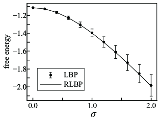
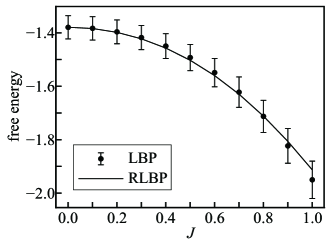
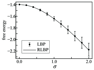
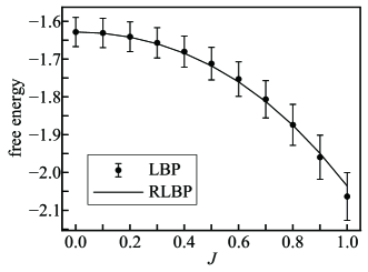
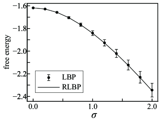
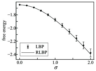
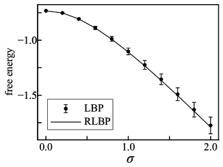
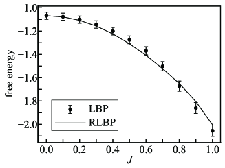
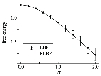
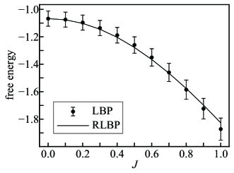
We show the results when the model in equation (34) is defined on a graph of an 8×8888\times 8 square lattice with the free boundary condition and when all of the interactions are unique, Jij=Jsubscript𝐽𝑖𝑗𝐽J_{ij}=J. Figures 46 show the plots for q=2𝑞2q=2, q=3𝑞3q=3, and q=4𝑞4q=4. “LBP” represents the results obtained by the numerically averaged Bethe free energy, and “RLBP” represents the results obtained by our method. Each plot of LBP is numerically averaged over 10000 realizations of the random fields.
Refer to caption
Refer to caption
Figure 4: Quenched Bethe free energies per variable for q=2𝑞2q=2. The left panel shows the free energies versus σ𝜎\sigma with J=0.2𝐽0.2J=0.2, and the right panel shows the free energies versus J𝐽J with σ=1𝜎1\sigma=1. The error bars are the standard deviation.
Refer to caption
Refer to caption
Figure 5: Quenched Bethe free energies per variable for q=3𝑞3q=3. The left panel shows the free energies versus σ𝜎\sigma with J=0.2𝐽0.2J=0.2, and the right panel shows the free energies versus J𝐽J with σ=1𝜎1\sigma=1. The error bars are the standard deviation.
Refer to caption
Refer to caption
Figure 6: Quenched Bethe free energies per variable for q=4𝑞4q=4. The left panel shows the free energies versus σ𝜎\sigma with J=0.2𝐽0.2J=0.2, and the right panel shows the free energies versus J𝐽J with σ=1𝜎1\sigma=1. The error bars are the standard deviation.

In almost all cases, the results of our method are consistent with the numerically averaged Bethe free energies, as expected. However, in the cases of large J𝐽J, mismatches between the two methods are observed.

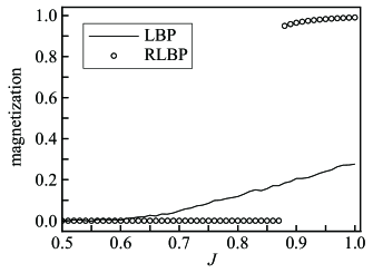
Figure 7 shows the plot of the quenched average of the magnetizations, MLBPsubscript𝑀LBPM_{\mathrm{LBP}} and MRLBPsubscript𝑀RLBPM_{\mathrm{RLBP}}, when the model shown in equation (34) is defined on a graph of a 14×14141414\times 14 square lattice with periodic boundary conditions and when q=2𝑞2q=2.

Refer to caption
Figure 7: Quenched magnetizations versus J𝐽J, where q=2𝑞2q=2 and σ=1𝜎1\sigma=1.

We observe that the two methods show the different nature of the magnetizations. The magnetization obtained by standard LBP continuously increases with the increase in J𝐽J, whereas that obtained by the proposed method drastically increases, like a first-order transition, around J0.88𝐽0.88J\approx 0.88. This different physical picture probably causes the mismatches between the two methods in the cases of large J𝐽J in figures 46.

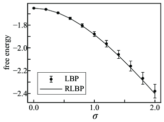
Our formulation allows for the approximate evaluation of the quenched average of Bethe free energy over the random fields with disordered interactions. We show the results when the model in equation (34) is defined on a graph of a 14×14141414\times 14 square lattice with free boundary conditions and when the interactions {Jij}subscript𝐽𝑖𝑗\{J_{ij}\} are independently drawn from 𝒩(Jij0,δ2)𝒩conditionalsubscript𝐽𝑖𝑗0superscript𝛿2\mathcal{N}(J_{ij}\mid 0,\delta^{2}). Figure 8 shows the results of the free energies versus σ𝜎\sigma for q=5𝑞5q=5.

Refer to caption
Refer to caption
Figure 8: Quenched Bethe free energies per variable versus σ𝜎\sigma for q=5𝑞5q=5. The left panel shows the free energies when δ=0.2𝛿0.2\delta=0.2, and the right panel shows the free energies when δ=0.4𝛿0.4\delta=0.4. The error bars are the standard deviation.

Each plot obtained by LBP is numerically averaged over 100 realizations of the random fields and over 200 realizations of the interactions, and that obtained by our method is averaged over 200 realizations of the interactions. Since the error bars of our method are quite small compared to LBP, we omit them in the figure. The results obtained by our method are consistent with the numerically averaged Bethe free energies.

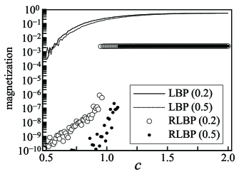
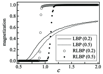
To see the effect of the disorder in the interactions on the behavior of the magnetization, we show the plot of the quenched average of the magnetizations when the model shown in equation (34) is defined on a graph of a 14×14141414\times 14 square lattice with periodic boundary conditions and when q=2𝑞2q=2 and the interactions {Jij}subscript𝐽𝑖𝑗\{J_{ij}\} are independently drawn from 𝒩(Jijc,δ2)𝒩conditionalsubscript𝐽𝑖𝑗𝑐superscript𝛿2\mathcal{N}(J_{ij}\mid c,\delta^{2}) in figure 9.

Refer to caption
Figure 9: Quenched magnetizations versus c𝑐c for δ=0.2𝛿0.2\delta=0.2 and δ=0.5𝛿0.5\delta=0.5 when q=2𝑞2q=2 and σ=1𝜎1\sigma=1.

We observe that the magnetizations obtained by our method show the first-order transition, as in figure 7. However, the values of the magnetizations after the transition are quite small compared to those in figure 7.

III.4.2 Random Regular Graph

A random regular graph (RRG) is a random graph in which the degrees of all vertices are fixed by the constant d𝑑d.

Refer to caption
Refer to caption
Figure 10: Quenched Bethe free energies per variable for q=2𝑞2q=2 on the RRG. The left panel shows the free energies versus σ𝜎\sigma with J=0.2𝐽0.2J=0.2, and the right panel shows the free energies versus J𝐽J with σ=1𝜎1\sigma=1. The error bars are the standard deviation.

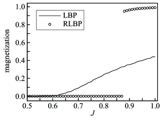
Figure 10 shows the results when the model in equation (34) is defined on an RRG with 200 vertices and d=4𝑑4d=4 and when Jij=Jsubscript𝐽𝑖𝑗𝐽J_{ij}=J and q=2𝑞2q=2. Each plot obtained by LBP is numerically averaged over 100 realizations of the random fields and over 100 realizations of the structure of graph, and that obtained by our method is averaged over 100 realizations of the structure of graph. Since the error bars of our method are quite small compared to LBP, we omit them in the figure, as in figure 8. The behaviors of the quenched magnetizations, MLBPsubscript𝑀LBPM_{\mathrm{LBP}} and MRLBPsubscript𝑀RLBPM_{\mathrm{RLBP}}, obtained by the two methods in this case are shown in figure 11.
Refer to caption
Figure 11: Quenched magnetizations versus J𝐽J on the RRG, where q=2𝑞2q=2 and σ=1𝜎1\sigma=1.

The behaviors of the quenched magnetizations in this figure are similar to those shown in figure 7.

LBP is asymptotically justified on an RRG Krzakala et al. (2010), because an RRG is quite sparse. Therefore, we can expect that the results obtained by LBP are close to the exact solutions. Except for the RS assumption, our method consists of two approximations: the approximation in equation (11) and the approximation in equation (19). Since the latter approximation is the Bethe approximation, it can be justified on a sparse graph such as an RRG. This suggests that the mismatch between the two methods in the right panel in figure 10 is mainly caused by the first approximation, and that the first approximation produces the metastable state that causes the first-order transition in figure 11.

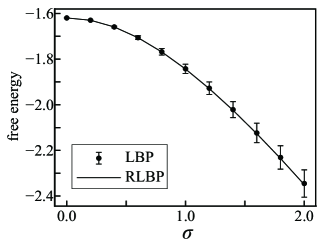
As in section III.4.1, we again see the case with the disordered interactions. Figure 12 shows the plots of the quenched Bethe free energies versus σ𝜎\sigma for q=5𝑞5q=5 when the model in equation (34) is defined on an RRG with 200 vertices and d=4𝑑4d=4 and when the interactions {Jij}subscript𝐽𝑖𝑗\{J_{ij}\} are independently drawn from 𝒩(Jij0,δ2)𝒩conditionalsubscript𝐽𝑖𝑗0superscript𝛿2\mathcal{N}(J_{ij}\mid 0,\delta^{2}). Each plot in the figure is obtained in the same manner as the case in figure 8.
Refer to caption
Refer to caption
Figure 12: Quenched Bethe free energies per variable versus σ𝜎\sigma for q=5𝑞5q=5 on the RRG. The left panel shows the free energies when δ=0.2𝛿0.2\delta=0.2, and the right panel shows the free energies when δ=0.4𝛿0.4\delta=0.4. The error bars are the standard deviation.

As is the case in figure 8, the results of our method are consistent with the numerically averaged Bethe free energies. Figure 13 shows the plot of the quenched average of the magnetizations when the model in equation (34) is defined on an RRG with 200 vertices and d=4𝑑4d=4 and when q=2𝑞2q=2 and {Jij}subscript𝐽𝑖𝑗\{J_{ij}\} are independently drawn from 𝒩(Jijc,δ2)𝒩conditionalsubscript𝐽𝑖𝑗𝑐superscript𝛿2\mathcal{N}(J_{ij}\mid c,\delta^{2}).

Refer to caption
Figure 13: Quenched magnetizations versus c𝑐c on the RRG for δ=0.2𝛿0.2\delta=0.2 and δ=0.5𝛿0.5\delta=0.5 when q=2𝑞2q=2 and σ=1𝜎1\sigma=1.

It can be observed that the transition of the magnetization obtained by our method is nearly continuous with the increase in the magnitude of the disorder. This suggests that the disorder in the interactions violates the metastable state of the quenched Bethe free energy obtained by our method in the case of an RRG.

III.5 Exactly Solvable Case – Ferromagnetic Mean-field Model in Random Fields

In this section, we consider the ferromagnetic mean-field model in random fields expressed as Schneider and Pytte (1977)

P(𝑺𝒉,β)expβ(iVϕ(Si,hi)+1ni<jg(Si)g(Sj)),proportional-to𝑃conditional𝑺𝒉𝛽𝛽subscript𝑖𝑉italic-ϕsubscript𝑆𝑖subscript𝑖1𝑛subscript𝑖𝑗𝑔subscript𝑆𝑖𝑔subscript𝑆𝑗\displaystyle P(\bm{S}\mid\bm{h},\beta)\propto\exp\beta\Big{(}\sum_{i\in V}\phi(S_{i},h_{i})+\frac{1}{n}\sum_{i<j}g(S_{i})g(S_{j})\Big{)}, (35)

where the second summation represents the summation over all of the distinct pairs of vertices, and {hi}subscript𝑖\{h_{i}\} represents the i.i.d. random fields drawn from the distribution ph(hi)subscript𝑝subscript𝑖p_{h}(h_{i}). By using the Hubbard–Stratonovich transformation, the free energy (per variable) of this model, f:=F(𝒉,β)/nassign𝑓𝐹𝒉𝛽𝑛f:=F(\bm{h},\beta)/n, can be expressed as

f𝑓\displaystyle f =1nβlndmexpn{β2m2\displaystyle=-\frac{1}{n\beta}\ln\int\mathrm{d}m\exp n\Big{\{}-\frac{\beta}{2}m^{2}
+1niVlnSexpβ(ϕ(S,hi)+mg(S)g(S)22n)}\displaystyle\quad\>+\frac{1}{n}\sum_{i\in V}\ln\sum_{S}\exp\beta\Big{(}\phi(S,h_{i})+mg(S)-\frac{g(S)^{2}}{2n}\Big{)}\Big{\}}
12nβlnnβ2π.12𝑛𝛽𝑛𝛽2𝜋\displaystyle\quad\>-\frac{1}{2n\beta}\ln\frac{n\beta}{2\pi}.

For a sufficiently large n𝑛n, we can compute the integration by using the saddle point method and the summation over iV𝑖𝑉i\in V in the exponent by using the law of large numbers, so that the free energy can be expressed as

f𝑓\displaystyle f =β2m21βdhph(h)lnSexpβ(ϕ(S,h)+mg(S))absent𝛽2superscript𝑚21𝛽differential-dsubscript𝑝subscript𝑆𝛽italic-ϕ𝑆𝑚𝑔𝑆\displaystyle=\frac{\beta}{2}m^{2}-\frac{1}{\beta}\int\mathrm{d}h\,p_{h}(h)\ln\sum_{S}\exp\beta\big{(}\phi(S,h)+mg(S)\big{)} (36)

in the thermodynamic limit, where m𝑚m is the solution to the saddle point equation:

m=dhph(h)Sg(S)expβ(ϕ(S,h)+mg(S))Sexpβ(ϕ(S,h)+mg(S)).𝑚differential-dsubscript𝑝subscript𝑆𝑔𝑆𝛽italic-ϕ𝑆𝑚𝑔𝑆subscript𝑆𝛽italic-ϕ𝑆𝑚𝑔𝑆\displaystyle m=\int\mathrm{d}h\,p_{h}(h)\frac{\sum_{S}g(S)\exp\beta\big{(}\phi(S,h)+mg(S)\big{)}}{\sum_{S}\exp\beta\big{(}\phi(S,h)+mg(S)\big{)}}. (37)

Since the free energy in equation (36) does not depend on {hi}subscript𝑖\{h_{i}\}, the quenched average of the free energy over the random fields, [F]𝒉/nsubscriptdelimited-[]𝐹𝒉𝑛[F]_{\bm{h}}/n, coincides with equation (36).

Since ψi,j(Si,Sj)=g(Si)g(Sj)/nsubscript𝜓𝑖𝑗subscript𝑆𝑖subscript𝑆𝑗𝑔subscript𝑆𝑖𝑔subscript𝑆𝑗𝑛\psi_{i,j}(S_{i},S_{j})=g(S_{i})g(S_{j})/n, the message-passing equation in equation (26) can be expanded as

lnμji(Si)subscript𝜇𝑗𝑖subscript𝑆𝑖\displaystyle\ln\mu_{j\to i}(S_{i})
=lnSjQj(Sj)exp(βψi,j(Si,Sj))μij(Sj)1+c0absentsubscriptsubscript𝑆𝑗subscript𝑄𝑗subscript𝑆𝑗𝛽subscript𝜓𝑖𝑗subscript𝑆𝑖subscript𝑆𝑗subscript𝜇𝑖𝑗superscriptsubscript𝑆𝑗1subscript𝑐0\displaystyle=\ln\sum_{S_{j}}Q_{j}(S_{j})\exp\big{(}\beta\psi_{i,j}(S_{i},S_{j})\big{)}\mu_{i\to j}(S_{j})^{-1}+c_{0}
=βng(Si)Sjg(Sj)Qj(Sj)μij(Sj)1SjQj(Sj)μij(Sj)1+c1+O(n2),absent𝛽𝑛𝑔subscript𝑆𝑖subscriptsubscript𝑆𝑗𝑔subscript𝑆𝑗subscript𝑄𝑗subscript𝑆𝑗subscript𝜇𝑖𝑗superscriptsubscript𝑆𝑗1subscriptsubscript𝑆𝑗subscript𝑄𝑗subscript𝑆𝑗subscript𝜇𝑖𝑗superscriptsubscript𝑆𝑗1subscript𝑐1𝑂superscript𝑛2\displaystyle=\frac{\beta}{n}\frac{g(S_{i})\sum_{S_{j}}g(S_{j})Q_{j}(S_{j})\mu_{i\to j}(S_{j})^{-1}}{\sum_{S_{j}}Q_{j}(S_{j})\mu_{i\to j}(S_{j})^{-1}}+c_{1}+O(n^{-2}), (38)

where c0subscript𝑐0c_{0} and c1subscript𝑐1c_{1} are constants unrelated to Sisubscript𝑆𝑖S_{i}. From this equation, we ensure that all of the messages are constants unrelated to 𝑺𝑺\bm{S} for a sufficiently large n𝑛n, because μji(Si)=exp(c1+O(n1))exp(c1)subscript𝜇𝑗𝑖subscript𝑆𝑖subscript𝑐1𝑂superscript𝑛1similar-to-or-equalssubscript𝑐1\mu_{j\to i}(S_{i})=\exp(c_{1}+O(n^{-1}))\simeq\exp(c_{1}). Therefore, from equations (28) and (38), we obtain

Λi(Si)=g(Si)njiSjg(Sj)Qj(Sj)+c2=mg(Si)+c2subscriptΛ𝑖subscript𝑆𝑖𝑔subscript𝑆𝑖𝑛subscript𝑗𝑖subscriptsubscript𝑆𝑗𝑔subscript𝑆𝑗subscript𝑄𝑗subscript𝑆𝑗subscript𝑐2𝑚𝑔subscript𝑆𝑖subscript𝑐2\displaystyle\Lambda_{i}(S_{i})=\frac{g(S_{i})}{n}\sum_{j\in\partial i}\sum_{S_{j}}g(S_{j})Q_{j}(S_{j})+c_{2}=mg(S_{i})+c_{2} (39)

for a sufficiently large n𝑛n, where c2subscript𝑐2c_{2} is a constant unrelated to Sisubscript𝑆𝑖S_{i}, and we redefine m:=n1iVSig(Si)Qj(Si)assign𝑚superscript𝑛1subscript𝑖𝑉subscriptsubscript𝑆𝑖𝑔subscript𝑆𝑖subscript𝑄𝑗subscript𝑆𝑖m:=n^{-1}\sum_{i\in V}\sum_{S_{i}}g(S_{i})Q_{j}(S_{i}). By substituting equation (39) into equation (27), we obtain the same expression for m𝑚m as equation (37). Since all of the messages are constants, from equation (29), we have

Qi,j(Si,Sj)=Qi(Si)Qj(Sj).subscript𝑄𝑖𝑗subscript𝑆𝑖subscript𝑆𝑗subscript𝑄𝑖subscript𝑆𝑖subscript𝑄𝑗subscript𝑆𝑗\displaystyle Q_{i,j}(S_{i},S_{j})=Q_{i}(S_{i})Q_{j}(S_{j}).

By substituting this equation and equation (39) into equation (21), we find that the equality f=minLBP(RS)/n𝑓superscriptsubscriptminLBPRS𝑛f=\mathcal{F}_{\mathrm{min}}^{\mathrm{LBP(RS)}}/n holds in the thermodynamic limit. From this result, we can conclude that our message-passing method can exactly compute the quenched average of the free energy of the model in equation (35) in the thermodynamic limit.

IV Application to Bayesian Image Restoration

In this section, we describe the estimation of the statistical performance of the Bayesian image restoration system using LBP by using the proposed method. In images, each pixel is allocated in a two-dimensional grid and has an intensity value corresponding to the color at its position. For an image 𝑰{IiiV}𝑰conditional-setsubscript𝐼𝑖𝑖𝑉\bm{I}\in\{I_{i}\mid i\in V\}, the entry Ii{0,1,,q1}subscript𝐼𝑖01𝑞1I_{i}\in\{0,1,\ldots,q-1\} represents the intensity of the i𝑖ith pixel.

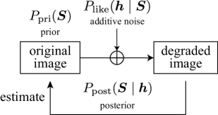
Suppose that the original image 𝑰𝑰\bm{I} is degraded to 𝒉𝒉\bm{h} through a specific noise process. In the Bayesian image restoration system, we assume that the original image is the sample drawn from the specific distribution Ppri(𝑺)subscript𝑃pri𝑺P_{\mathrm{pri}}(\bm{S}) known as the prior distribution. We observe only the degraded image as the input, and we want to estimate the original image from the input degraded image. To do the image restoration, we compute the posterior distribution of the original image, Ppost(𝑺𝒉)Plike(𝒉𝑺)Ppri(𝑺)proportional-tosubscript𝑃postconditional𝑺𝒉subscript𝑃likeconditional𝒉𝑺subscript𝑃pri𝑺P_{\mathrm{post}}(\bm{S}\mid\bm{h})\propto P_{\mathrm{like}}(\bm{h}\mid\bm{S})P_{\mathrm{pri}}(\bm{S}), where Plike(𝒉𝑺)subscript𝑃likeconditional𝒉𝑺P_{\mathrm{like}}(\bm{h}\mid\bm{S}) is the noise process referred to as the likelihood. We use the posterior distribution to produce the restored image as the output. The scheme of Bayesian image restoration is shown in figure 14.
Refer to caption
Figure 14: Scheme of Bayesian image restoration.

IV.1 Bayesian Image Restoration using LBP

For the original image 𝑰𝑰\bm{I}, suppose that the degraded image 𝒉𝒉\bm{h} is generated by adding additive white Gaussian noise, i.e., hi=Ii+ηisubscript𝑖subscript𝐼𝑖subscript𝜂𝑖h_{i}=I_{i}+\eta_{i}, where ηisubscript𝜂𝑖\eta_{i} is the random noise drawn from the Gaussian distribution 𝒩(η0,σ2)𝒩conditional𝜂0superscript𝜎2\mathcal{N}(\eta\mid 0,\sigma^{2}).

We define the prior distribution of the images 𝑺𝑺\bm{S} as

Ppri(𝑺α)exp(α{i,j}Eξ(Si,Sj)),proportional-tosubscript𝑃priconditional𝑺𝛼𝛼subscript𝑖𝑗𝐸𝜉subscript𝑆𝑖subscript𝑆𝑗\displaystyle P_{\mathrm{pri}}(\bm{S}\mid\alpha)\propto\exp\Big{(}\alpha\sum_{\{i,j\}\in E}\xi(S_{i},S_{j})\Big{)}, (40)

which is defined on a square lattice corresponding to the configuration of pixels. The energy function ξ(Si,Sj)𝜉subscript𝑆𝑖subscript𝑆𝑗\xi(S_{i},S_{j}) defines the relationship among neighboring pixels, and it often takes a form that emphasizes the smoothness among neighboring pixels, e.g., ξ(Si,Sj)=|SiSi|𝜉subscript𝑆𝑖subscript𝑆𝑗subscript𝑆𝑖subscript𝑆𝑖\xi(S_{i},S_{j})=-|S_{i}-S_{i}|. The positive parameter α𝛼\alpha controls the strength of the smoothness. For the original image, the distribution of the degraded image, i.e., the likelihood, is expressed as

Plike(𝒉𝑺=𝑰,σ2)=iV𝒩(hiIi,σ2).subscript𝑃likeconditional𝒉𝑺𝑰superscript𝜎2subscriptproduct𝑖𝑉𝒩conditionalsubscript𝑖subscript𝐼𝑖superscript𝜎2\displaystyle P_{\mathrm{like}}(\bm{h}\mid\bm{S}=\bm{I},\sigma^{2})=\prod_{i\in V}\mathcal{N}(h_{i}\mid I_{i},\sigma^{2}). (41)

From equations (40) and (41), given a specific degraded image 𝒉𝒉\bm{h}, the posterior distribution of the original image is obtained by

Ppost(𝑺𝒉,α,σ2)Plike(𝒉𝑺,σ2)Ppri(𝑺α)proportional-tosubscript𝑃postconditional𝑺𝒉𝛼superscript𝜎2subscript𝑃likeconditional𝒉𝑺superscript𝜎2subscript𝑃priconditional𝑺𝛼\displaystyle P_{\mathrm{post}}(\bm{S}\mid\bm{h},\alpha,\sigma^{2})\propto P_{\mathrm{like}}(\bm{h}\mid\bm{S},\sigma^{2})P_{\mathrm{pri}}(\bm{S}\mid\alpha)
exp(iV(Sihi)22σ2+α{i,j}Eξ(Si,Sj)).proportional-toabsentsubscript𝑖𝑉superscriptsubscript𝑆𝑖subscript𝑖22superscript𝜎2𝛼subscript𝑖𝑗𝐸𝜉subscript𝑆𝑖subscript𝑆𝑗\displaystyle\propto\exp\Big{(}-\sum_{i\in V}\frac{(S_{i}-h_{i})^{2}}{2\sigma^{2}}+\alpha\sum_{\{i,j\}\in E}\xi(S_{i},S_{j})\Big{)}. (42)

The posterior distribution is the special case of equation (1). The degraded image is regarded as the random fields in the posterior distribution.

In maximum posterior marginal (MPM) estimation, the i𝑖ith pixel of the restored image is obtained by

SiMPM:=argmaxSiPpost(Si𝒉,α,σ2),assignsuperscriptsubscript𝑆𝑖MPMargsubscriptsubscript𝑆𝑖subscript𝑃postconditionalsubscript𝑆𝑖𝒉𝛼superscript𝜎2\displaystyle S_{i}^{\mathrm{MPM}}:=\mathrm{arg}\max_{S_{i}}P_{\mathrm{post}}(S_{i}\mid\bm{h},\alpha,\sigma^{2}), (43)

where Ppost(Si𝒉,α,σ2)subscript𝑃postconditionalsubscript𝑆𝑖𝒉𝛼superscript𝜎2P_{\mathrm{post}}(S_{i}\mid\bm{h},\alpha,\sigma^{2}) is the marginal distribution of the posterior distribution in equation (42Tanaka (2002). In practice, we approximate the true marginal distributions by the beliefs obtained by LBP for the posterior distribution,

SiMPMSiMPM(LBP):=argmaxSibi(Si),superscriptsubscript𝑆𝑖MPMsuperscriptsubscript𝑆𝑖MPMLBPassignargsubscriptsubscript𝑆𝑖subscript𝑏𝑖subscript𝑆𝑖\displaystyle S_{i}^{\mathrm{MPM}}\approx S_{i}^{\mathrm{MPM(LBP)}}:=\mathrm{arg}\max_{S_{i}}b_{i}(S_{i}), (44)

where the belief bi(Si)subscript𝑏𝑖subscript𝑆𝑖b_{i}(S_{i}) is obtained by LBP described in section II.2 with ϕi(Si,hi)=(Sihi)2/2σ2subscriptitalic-ϕ𝑖subscript𝑆𝑖subscript𝑖superscriptsubscript𝑆𝑖subscript𝑖22superscript𝜎2\phi_{i}(S_{i},h_{i})=-(S_{i}-h_{i})^{2}/2\sigma^{2}, ψi,j(Si,Sj)=αξ(Si,Sj)subscript𝜓𝑖𝑗subscript𝑆𝑖subscript𝑆𝑗𝛼𝜉subscript𝑆𝑖subscript𝑆𝑗\psi_{i,j}(S_{i},S_{j})=\alpha\xi(S_{i},S_{j}), and β=1𝛽1\beta=1. The performance of the restoration is often measured by the mean square error (MSE) between the original image and the restored image,

D(𝑰,𝒉,α,σ2):=1niV(IiSiMPM(LBP))2.assign𝐷𝑰𝒉𝛼superscript𝜎21𝑛subscript𝑖𝑉superscriptsubscript𝐼𝑖superscriptsubscript𝑆𝑖MPMLBP2\displaystyle D(\bm{I},\bm{h},\alpha,\sigma^{2}):=\frac{1}{n}\sum_{i\in V}\big{(}I_{i}-S_{i}^{\mathrm{MPM(LBP)}}\big{)}^{2}. (45)

This MSE is for the specific input degraded image that is drawn from the likelihood in equation (41), and it should take different values for different degraded images in general.

For the original image 𝑰𝑰\bm{I}, we attempt to estimate the average value of the MSE in equation (45) over all possible degraded images,

Dav(𝑰,α,σ2):=[D(𝑰,𝒉,α,σ2)]𝒉,assignsubscript𝐷av𝑰𝛼superscript𝜎2subscriptdelimited-[]𝐷𝑰𝒉𝛼superscript𝜎2𝒉\displaystyle D_{\mathrm{av}}(\bm{I},\alpha,\sigma^{2}):=\big{[}D(\bm{I},\bm{h},\alpha,\sigma^{2})\big{]}_{\bm{h}}, (46)

where pi(h)=𝒩(hIi,σ2)subscript𝑝𝑖𝒩conditionalsubscript𝐼𝑖superscript𝜎2p_{i}(h)=\mathcal{N}(h\mid I_{i},\sigma^{2}), because the average value corresponds to the statistical performance of the presented Bayesian restoration system for the original image. By considering the input degraded image as the quenched parameter, the right-hand side of equation (46) can be regarded as the quenched average of the MSE obtained by LBP. Thus, we approximate it using the message-passing method presented in section III.3.

Using the proposed message-passing method, we approximate equation (46) as

Dav(𝑰,α,σ2)1niVdh𝒩(hIi,σ2)(Iiri(h))2,subscript𝐷av𝑰𝛼superscript𝜎21𝑛subscript𝑖𝑉differential-d𝒩conditionalsubscript𝐼𝑖superscript𝜎2superscriptsubscript𝐼𝑖subscript𝑟𝑖2\displaystyle D_{\mathrm{av}}(\bm{I},\alpha,\sigma^{2})\approx\frac{1}{n}\sum_{i\in V}\int\mathrm{d}h\,\mathcal{N}(h\mid I_{i},\sigma^{2})\big{(}I_{i}-r_{i}(h)\big{)}^{2}, (47)

where

ri(h)=argmaxS(ϕi(S,h)+Λi(S)).subscript𝑟𝑖argsubscript𝑆subscriptitalic-ϕ𝑖𝑆subscriptΛ𝑖𝑆\displaystyle r_{i}(h)=\mathrm{arg}\max_{S}\big{(}\phi_{i}(S,h)+\Lambda_{i}(S)\big{)}.

The detailed derivation of this approximation is shown in appendix C.

IV.2 Numerical Experiment

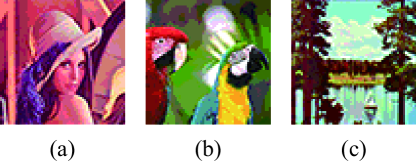
In this section, we describe the estimation of the performance of Bayesian image restoration for the 64×64646464\times 64 original colored images shown in figure 15. Colored images consist of three different channels: red, green, and blue (RGB) channels, 𝑰={𝑰red,𝑰green,𝑰blue}𝑰subscript𝑰redsubscript𝑰greensubscript𝑰blue\bm{I}=\{\bm{I}_{\mathrm{red}},\bm{I}_{\mathrm{green}},\bm{I}_{\mathrm{blue}}\}. The pixels in each channel in the original images have eight intensities, i.e., q=8𝑞8q=8. In the following experiments, we assume that the three different channels are independently degraded by the same noise process in equation (41), and we restore the generated degraded images, 𝒉={𝒉red,𝒉green,𝒉blue}𝒉subscript𝒉redsubscript𝒉greensubscript𝒉blue\bm{h}=\{\bm{h}_{\mathrm{red}},\bm{h}_{\mathrm{green}},\bm{h}_{\mathrm{blue}}\}, by separately applying the Bayesian image restoration based on the posterior distribution in equation (42) to the RGB channels. The value of σ2superscript𝜎2\sigma^{2} used in the restoration is the same as that used in the noise process, and we use the same values of the parameters, α𝛼\alpha and σ2superscript𝜎2\sigma^{2}, in the restorations for the three different channels. The total MSE of the restoration is obtained by the average of the MSEs of the RGB channels, i.e., D(𝑰,𝒉,α,σ2)={D(𝑰red,𝒉red,α,σ2)+D(𝑰green,𝒉green,α,σ2)+D(𝑰blue,𝒉blue,α,σ2)}/3𝐷𝑰𝒉𝛼superscript𝜎2𝐷subscript𝑰redsubscript𝒉red𝛼superscript𝜎2𝐷subscript𝑰greensubscript𝒉green𝛼superscript𝜎2𝐷subscript𝑰bluesubscript𝒉blue𝛼superscript𝜎23D(\bm{I},\bm{h},\alpha,\sigma^{2})=\{D(\bm{I}_{\mathrm{red}},\bm{h}_{\mathrm{red}},\alpha,\sigma^{2})+D(\bm{I}_{\mathrm{green}},\bm{h}_{\mathrm{green}},\alpha,\sigma^{2})+D(\bm{I}_{\mathrm{blue}},\bm{h}_{\mathrm{blue}},\alpha,\sigma^{2})\}/3.

Refer to caption
Figure 15: Original 3-bit colored images 𝑰𝑰\bm{I}: (a) lenna, (b) parrots, and (c) sailboat.

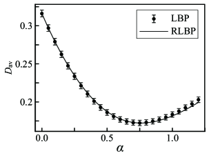
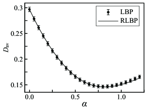
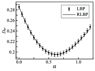
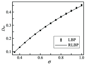
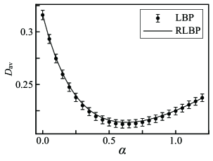
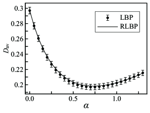
For the original colored images in figure 15, we evaluated the average of the MSE, Dav(𝑰,α,σ2)subscript𝐷av𝑰𝛼superscript𝜎2D_{\mathrm{av}}(\bm{I},\alpha,\sigma^{2}), by using two types of methods: LBP and the proposed analytical method in equation (47). In LBP, we approximated Dav(𝑰,α,σ2)subscript𝐷av𝑰𝛼superscript𝜎2D_{\mathrm{av}}(\bm{I},\alpha,\sigma^{2}) by the sample average of D(𝑰,𝒉,α,σ2)𝐷𝑰𝒉𝛼superscript𝜎2D(\bm{I},\bm{h},\alpha,\sigma^{2}) over 10000 different degraded images, which are generated from the original image 𝑰𝑰\bm{I} through the noise process shown in equation (41).

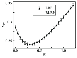
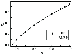
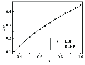
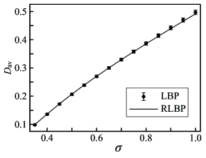
At first, we show the results obtained by setting the function ξ(Si,Sj)𝜉subscript𝑆𝑖subscript𝑆𝑗\xi(S_{i},S_{j}) as ξ(Si,Sj)=(SiSj)2/2𝜉subscript𝑆𝑖subscript𝑆𝑗superscriptsubscript𝑆𝑖subscript𝑆𝑗22\xi(S_{i},S_{j})=-(S_{i}-S_{j})^{2}/2 in the prior distribution in equation (40). In figures 16 and 17, we show the plots of Dav(𝑰,α,σ2)subscript𝐷av𝑰𝛼superscript𝜎2D_{\mathrm{av}}(\bm{I},\alpha,\sigma^{2}) versus α𝛼\alpha and σ𝜎\sigma, respectively, obtained by the two different methods: the sample average of the LBP restorations, “LBP,” and the proposed analytical method, “RLBP.” Figure 16 shows the plots of Dav(𝑰,α,σ2)subscript𝐷av𝑰𝛼superscript𝜎2D_{\mathrm{av}}(\bm{I},\alpha,\sigma^{2}) versus α𝛼\alpha when σ=0.5𝜎0.5\sigma=0.5, and figure 17 shows the plots of Dav(𝑰,α,σ2)subscript𝐷av𝑰𝛼superscript𝜎2D_{\mathrm{av}}(\bm{I},\alpha,\sigma^{2}) versus σ𝜎\sigma when α=0.4𝛼0.4\alpha=0.4. Each plot obtained by LBP restoration is averaged over 10000 realizations of the stochastically generated degraded image.
Refer to caption
Refer to caption
Refer to caption
Figure 16: Plots of Dav(𝑰,α,σ2)subscript𝐷av𝑰𝛼superscript𝜎2D_{\mathrm{av}}(\bm{I},\alpha,\sigma^{2}) versus α𝛼\alpha when σ=0.5𝜎0.5\sigma=0.5 and ξ(Si,Sj)=(SiSj)2/2𝜉subscript𝑆𝑖subscript𝑆𝑗superscriptsubscript𝑆𝑖subscript𝑆𝑗22\xi(S_{i},S_{j})=-(S_{i}-S_{j})^{2}/2 for the original images shown in figure 15: the left, middle, and right plots show the results for figures 15(a), 15(b), and 15(c), respectively. The error bars are the standard deviation.
Refer to caption
Refer to caption
Refer to caption
Figure 17: Plots of Dav(𝑰,α,σ2)subscript𝐷av𝑰𝛼superscript𝜎2D_{\mathrm{av}}(\bm{I},\alpha,\sigma^{2}) versus σ𝜎\sigma when α=0.4𝛼0.4\alpha=0.4 and ξ(Si,Sj)=(SiSj)2/2𝜉subscript𝑆𝑖subscript𝑆𝑗superscriptsubscript𝑆𝑖subscript𝑆𝑗22\xi(S_{i},S_{j})=-(S_{i}-S_{j})^{2}/2 for the original images shown in figure 15: the left, middle and right plots show the results for figures 15(a), 15(b), and 15(c), respectively. The error bars are the standard deviation.

We can observe that the results obtained by our method in equation (47) are in good agreement with those obtained by LBP restoration.

Next, we show the results obtained by setting the function ξ(Si,Sj)𝜉subscript𝑆𝑖subscript𝑆𝑗\xi(S_{i},S_{j}) as ξ(Si,Sj)=|SiSj|2𝜉subscript𝑆𝑖subscript𝑆𝑗superscriptsubscript𝑆𝑖subscript𝑆𝑗2\xi(S_{i},S_{j})=-|S_{i}-S_{j}|^{2}.

Refer to caption
Refer to caption
Refer to caption
Figure 18: Plots of Dav(𝑰,α,σ2)subscript𝐷av𝑰𝛼superscript𝜎2D_{\mathrm{av}}(\bm{I},\alpha,\sigma^{2}) versus α𝛼\alpha when σ=0.5𝜎0.5\sigma=0.5 and ξ(Si,Sj)=|SiSj|𝜉subscript𝑆𝑖subscript𝑆𝑗subscript𝑆𝑖subscript𝑆𝑗\xi(S_{i},S_{j})=-|S_{i}-S_{j}| for the original images shown in figure 15: the left, middle, and right plots show the results for figures 15(a), 15(b), and 15(c), respectively. The error bars are the standard deviation.
Refer to caption
Refer to caption
Refer to caption
Figure 19: Plots of Dav(𝑰,α,σ2)subscript𝐷av𝑰𝛼superscript𝜎2D_{\mathrm{av}}(\bm{I},\alpha,\sigma^{2}) versus σ𝜎\sigma when α=0.4𝛼0.4\alpha=0.4 and ξ(Si,Sj)=|SiSj|𝜉subscript𝑆𝑖subscript𝑆𝑗subscript𝑆𝑖subscript𝑆𝑗\xi(S_{i},S_{j})=-|S_{i}-S_{j}| for the original images shown in figure 15: the left, middle, and right plots show the results for figure 15(a), 15(b), and 15(c), respectively. The error bars are the standard deviation.

Figure 18 shows the plots of Dav(𝑰,α,σ2)subscript𝐷av𝑰𝛼superscript𝜎2D_{\mathrm{av}}(\bm{I},\alpha,\sigma^{2}) versus α𝛼\alpha when σ=0.5𝜎0.5\sigma=0.5, and figure 19 shows the plots of Dav(𝑰,α,σ2)subscript𝐷av𝑰𝛼superscript𝜎2D_{\mathrm{av}}(\bm{I},\alpha,\sigma^{2}) versus σ𝜎\sigma when α=0.4𝛼0.4\alpha=0.4. The results obtained by our method are in good agreement with those obtained by LBP restoration in figures 16 and 17.

V Conclusion and Remarks

In this paper, we proposed an analytical method based on the idea of the RCVM to approximately evaluate the quenched average of the Bethe free energy, obtained by LBP, of the pair-wise MRF in equation (1) in random fields 𝒉𝒉\bm{h}. Since our message-passing-type formulation allows any form of the functions ϕi(Si,hi)subscriptitalic-ϕ𝑖subscript𝑆𝑖subscript𝑖\phi_{i}(S_{i},h_{i}) and ψi,j(Si,Sj)subscript𝜓𝑖𝑗subscript𝑆𝑖subscript𝑆𝑗\psi_{i,j}(S_{i},S_{j}) in the Hamiltonian and allows any form of the distributions of the random fields {pi(hi)}subscript𝑝𝑖subscript𝑖\{p_{i}(h_{i})\}, except for the cases where correlations among fields exist, the proposed method is applicable to a wide range of applications in physics and in computer science. In the argument in section III.5, we found that this approximation is justified in the ferromagnetic mean-field model in random fields.

Although the results obtained by our analytical method in almost all cases were consistent with those obtained by the numerical method, as seen in the artificial model presented in section III.4 and in the Bayesian image restoration presented in section IV.2, some mismatches, especially in the behaviors of the phase transitions of the magnetizations in section III.4, between the results obtained by our method and by the numerical method were observed. As mentioned in section III.4.2, the mismatches are considered to be mainly caused by the approximation based on the CVM in equation (11). However, a detailed understanding of its mathematical meaning is still unclear, even though it is one of the most important components of our method, because the approximation is for the system replicated by the replica method; thus, the development of a mathematical understanding of how it affects the present method is not straightforward. It should be considered in future studies.

We employed the Bethe approximation in equation (19) for the purpose of evaluating the quenched average of the Bethe free energy. Our approximate framework, however, allows us to employ other mean-field approximations instead of the Bethe approximation, and the resulting form can be expected to be an approximation of an employed approximation method. Thus, in accordance with the presented framework, it is expected that we can evaluate the quenched averages of the employed mean-field methods for random fields.

Appendix A Derivation of Equation (21)

By substituting equation (20) into equation (18), we obtain the Bethe approximation of xRCVM[{Qα,Qiα}]superscriptsubscript𝑥RCVMdelimited-[]superscript𝑄𝛼superscriptsubscript𝑄𝑖𝛼\mathcal{F}_{x}^{\mathrm{RCVM}}[\{Q^{\alpha},Q_{i}^{\alpha}\}] as

xLBP[{Qiα,Qi,jα}]:=iVextr𝚲i{α=1xSiαΛiα(Siα)Qiα(Siα)\displaystyle\mathcal{F}_{x}^{\mathrm{LBP}}[\{Q_{i}^{\alpha},Q_{i,j}^{\alpha}\}]:=\sum_{i\in V}\underset{\bm{\Lambda}_{i}}{\mathrm{extr}}\Big{\{}\sum_{\alpha=1}^{x}\sum_{S_{i}^{\alpha}}\Lambda_{i}^{\alpha}(S_{i}^{\alpha})Q_{i}^{\alpha}(S_{i}^{\alpha})
1βlndhpi(h)α=1xSiαexpβ(ϕi(Siα,h)+Λiα(Siα))}\displaystyle-\frac{1}{\beta}\ln\int\mathrm{d}h\,p_{i}(h)\prod_{\alpha=1}^{x}\sum_{S_{i}^{\alpha}}\exp\beta\big{(}\phi_{i}(S_{i}^{\alpha},h)+\Lambda_{i}^{\alpha}(S_{i}^{\alpha})\big{)}\Big{\}}
+α=1x𝒱intbethe[{Qiα,Qi,jα}]1βiVα=1x1[Qiα].superscriptsubscript𝛼1𝑥superscriptsubscript𝒱intbethedelimited-[]superscriptsubscript𝑄𝑖𝛼superscriptsubscript𝑄𝑖𝑗𝛼1𝛽subscript𝑖𝑉superscriptsubscript𝛼1𝑥subscript1delimited-[]superscriptsubscript𝑄𝑖𝛼\displaystyle+\sum_{\alpha=1}^{x}\mathcal{V}_{\mathrm{int}}^{\mathrm{bethe}}[\{Q_{i}^{\alpha},Q_{i,j}^{\alpha}\}]-\frac{1}{\beta}\sum_{i\in V}\sum_{\alpha=1}^{x}\mathcal{H}_{1}[Q_{i}^{\alpha}]. (48)

At the minimum point of this variational free energy, we make the RS assumption; that is, the relations Qiα(Si)=Qi(Si)superscriptsubscript𝑄𝑖𝛼subscript𝑆𝑖subscript𝑄𝑖subscript𝑆𝑖Q_{i}^{\alpha}(S_{i})=Q_{i}(S_{i}) and Qi,jα(Si,Sj)=Qi,j(Si,Sj)superscriptsubscript𝑄𝑖𝑗𝛼subscript𝑆𝑖subscript𝑆𝑗subscript𝑄𝑖𝑗subscript𝑆𝑖subscript𝑆𝑗Q_{i,j}^{\alpha}(S_{i},S_{j})=Q_{i,j}(S_{i},S_{j}) hold for any α𝛼\alpha. Under this assumption, the minimum of xLBP[{Qiα,Qi,jα}]superscriptsubscript𝑥LBPdelimited-[]superscriptsubscript𝑄𝑖𝛼superscriptsubscript𝑄𝑖𝑗𝛼\mathcal{F}_{x}^{\mathrm{LBP}}[\{Q_{i}^{\alpha},Q_{i,j}^{\alpha}\}] is equivalent to the minimum of the RS variational free energy expressed as

xLBP(RS)[{Qi,Qi,j}]:=iVextr𝚲i{α=1xSiαΛiα(Siα)Qi(Siα)\displaystyle\mathcal{F}_{x}^{\mathrm{LBP(RS)}}[\{Q_{i},Q_{i,j}\}]:=\sum_{i\in V}\underset{\bm{\Lambda}_{i}}{\mathrm{extr}}\Big{\{}\sum_{\alpha=1}^{x}\sum_{S_{i}^{\alpha}}\Lambda_{i}^{\alpha}(S_{i}^{\alpha})Q_{i}(S_{i}^{\alpha})
1βlndhpi(h)α=1xSiαexpβ(ϕi(Siα,h)+Λiα(Siα))}\displaystyle-\frac{1}{\beta}\ln\int\mathrm{d}h\,p_{i}(h)\prod_{\alpha=1}^{x}\sum_{S_{i}^{\alpha}}\exp\beta\big{(}\phi_{i}(S_{i}^{\alpha},h)+\Lambda_{i}^{\alpha}(S_{i}^{\alpha})\big{)}\Big{\}}
+x𝒱intbethe[{Qi,Qi,j}]xβiV1[Qi].𝑥superscriptsubscript𝒱intbethedelimited-[]subscript𝑄𝑖subscript𝑄𝑖𝑗𝑥𝛽subscript𝑖𝑉subscript1delimited-[]subscript𝑄𝑖\displaystyle+x\mathcal{V}_{\mathrm{int}}^{\mathrm{bethe}}[\{Q_{i},Q_{i,j}\}]-\frac{x}{\beta}\sum_{i\in V}\mathcal{H}_{1}[Q_{i}]. (49)

From the convexity of the first term of this equation with respect to 𝚲isubscript𝚲𝑖\bm{\Lambda}_{i} and the extremal conditions of 𝚲isubscript𝚲𝑖\bm{\Lambda}_{i}, it can be ensured that the relation Λiα(Si)=Λi(Si)superscriptsubscriptΛ𝑖𝛼subscript𝑆𝑖subscriptΛ𝑖subscript𝑆𝑖\Lambda_{i}^{\alpha}(S_{i})=\Lambda_{i}(S_{i}) holds for any α𝛼\alpha at the extremal points of 𝚲isubscript𝚲𝑖\bm{\Lambda}_{i}. Therefore, equation (49) can be reduced to

xLBP(RS)[{Qi,Qi,j}]=iVextrΛi{xSiΛi(Si)Qi(Si)\displaystyle\mathcal{F}_{x}^{\mathrm{LBP(RS)}}[\{Q_{i},Q_{i,j}\}]=\sum_{i\in V}\underset{\Lambda_{i}}{\mathrm{extr}}\Big{\{}x\sum_{S_{i}}\Lambda_{i}(S_{i})Q_{i}(S_{i})
1βlndhpi(h)exp(xlnSiexpβ(ϕi(Si,h)+Λi(Si)))}\displaystyle-\frac{1}{\beta}\ln\int\mathrm{d}h\,p_{i}(h)\exp\Big{(}x\ln\sum_{S_{i}}\exp\beta\big{(}\phi_{i}(S_{i},h)+\Lambda_{i}(S_{i})\big{)}\Big{)}\Big{\}}
+x𝒱intbethe[{Qi,Qi,j}]xβiV1[Qi],𝑥superscriptsubscript𝒱intbethedelimited-[]subscript𝑄𝑖subscript𝑄𝑖𝑗𝑥𝛽subscript𝑖𝑉subscript1delimited-[]subscript𝑄𝑖\displaystyle+x\mathcal{V}_{\mathrm{int}}^{\mathrm{bethe}}[\{Q_{i},Q_{i,j}\}]-\frac{x}{\beta}\sum_{i\in V}\mathcal{H}_{1}[Q_{i}], (50)

and we regard the minimum of this variational free energy as the Bethe approximation of the true x𝑥x-replicated free energy in equation (10).

From equations (9), (10), and (50), our desired variational free energy is obtained by

LBP(RS)[{Qi,Qi,j}]superscriptLBPRSdelimited-[]subscript𝑄𝑖subscript𝑄𝑖𝑗\displaystyle\mathcal{F}^{\mathrm{LBP(RS)}}[\{Q_{i},Q_{i,j}\}]
:=1βlimx0exp(βxLBP(RS)[{Qi,Qi,j}])1x.assignabsent1𝛽subscript𝑥0𝛽superscriptsubscript𝑥LBPRSdelimited-[]subscript𝑄𝑖subscript𝑄𝑖𝑗1𝑥\displaystyle:=-\frac{1}{\beta}\lim_{x\to 0}\frac{\exp(-\beta\mathcal{F}_{x}^{\mathrm{LBP(RS)}}[\{Q_{i},Q_{i,j}\}])-1}{x}. (51)

This leads to equation (21).

Appendix B Derivation of the Message-passing Equation

To perform the conditional minimization of the variational free energy in equation (21), we use the Lagrange multipliers as

LBP(RS)[{Qi,Qi,j}]superscriptLBPRSdelimited-[]subscript𝑄𝑖subscript𝑄𝑖𝑗\displaystyle\mathcal{L}^{\mathrm{LBP(RS)}}[\{Q_{i},Q_{i,j}\}] :=LBP(RS)[{Qi,Qi,j}]iVai(SiQi(Si)1){i,j}Ebi,j(Si,SjQi,j(Si,Sj)1)assignabsentsuperscriptLBPRSdelimited-[]subscript𝑄𝑖subscript𝑄𝑖𝑗subscript𝑖𝑉subscript𝑎𝑖subscriptsubscript𝑆𝑖subscript𝑄𝑖subscript𝑆𝑖1subscript𝑖𝑗𝐸subscript𝑏𝑖𝑗subscriptsubscript𝑆𝑖subscript𝑆𝑗subscript𝑄𝑖𝑗subscript𝑆𝑖subscript𝑆𝑗1\displaystyle:=\mathcal{F}^{\mathrm{LBP(RS)}}[\{Q_{i},Q_{i,j}\}]-\sum_{i\in V}a_{i}\Big{(}\sum_{S_{i}}Q_{i}(S_{i})-1\Big{)}-\sum_{\{i,j\}\in E}b_{i,j}\Big{(}\sum_{S_{i},S_{j}}Q_{i,j}(S_{i},S_{j})-1\Big{)}
{i,j}E{Siλj,i(Si)(SjQi,j(Si,Sj)Qi(Si))+Sjλi,j(Sj)(SiQi,j(Si,Sj)Qj(Sj))},subscript𝑖𝑗𝐸subscriptsubscript𝑆𝑖subscript𝜆𝑗𝑖subscript𝑆𝑖subscriptsubscript𝑆𝑗subscript𝑄𝑖𝑗subscript𝑆𝑖subscript𝑆𝑗subscript𝑄𝑖subscript𝑆𝑖subscriptsubscript𝑆𝑗subscript𝜆𝑖𝑗subscript𝑆𝑗subscriptsubscript𝑆𝑖subscript𝑄𝑖𝑗subscript𝑆𝑖subscript𝑆𝑗subscript𝑄𝑗subscript𝑆𝑗\displaystyle\quad\>-\sum_{\{i,j\}\in E}\Big{\{}\sum_{S_{i}}\lambda_{j,i}(S_{i})\Big{(}\sum_{S_{j}}Q_{i,j}(S_{i},S_{j})-Q_{i}(S_{i})\Big{)}+\sum_{S_{j}}\lambda_{i,j}(S_{j})\Big{(}\sum_{S_{i}}Q_{i,j}(S_{i},S_{j})-Q_{j}(S_{j})\Big{)}\Big{\}},

where the Lagrange multipliers, {ai,bi,j}subscript𝑎𝑖subscript𝑏𝑖𝑗\{a_{i},b_{i,j}\} and {λi,j(Sj)}subscript𝜆𝑖𝑗subscript𝑆𝑗\{\lambda_{i,j}(S_{j})\}, correspond to the normalization constraints in equation (23) and the marginal constraints in equations (24) and (25), respectively. From the minimum conditions of LBP(RS)[{Qi,Qi,j}]superscriptLBPRSdelimited-[]subscript𝑄𝑖subscript𝑄𝑖𝑗\mathcal{L}^{\mathrm{LBP(RS)}}[\{Q_{i},Q_{i,j}\}] with respect to Qi(Si)subscript𝑄𝑖subscript𝑆𝑖Q_{i}(S_{i}) and Qi,j(Si,Sj)subscript𝑄𝑖𝑗subscript𝑆𝑖subscript𝑆𝑗Q_{i,j}(S_{i},S_{j}), we obtain

Qi(Si)expβ|i|(Λi(Si)+kiλk,i(Si))proportional-tosubscript𝑄𝑖subscript𝑆𝑖𝛽𝑖subscriptΛ𝑖subscript𝑆𝑖subscript𝑘𝑖subscript𝜆𝑘𝑖subscript𝑆𝑖\displaystyle Q_{i}(S_{i})\propto\exp\frac{\beta}{|\partial i|}\Big{(}\Lambda_{i}(S_{i})+\sum_{k\in\partial i}\lambda_{k,i}(S_{i})\Big{)} (52)

and

Qi,j(Si,Sj)expβ(ψi,j(Si,Sj)+λi,j(Sj)+λj,i(Si)),proportional-tosubscript𝑄𝑖𝑗subscript𝑆𝑖subscript𝑆𝑗𝛽subscript𝜓𝑖𝑗subscript𝑆𝑖subscript𝑆𝑗subscript𝜆𝑖𝑗subscript𝑆𝑗subscript𝜆𝑗𝑖subscript𝑆𝑖\displaystyle Q_{i,j}(S_{i},S_{j})\propto\exp\beta\big{(}\psi_{i,j}(S_{i},S_{j})+\lambda_{i,j}(S_{j})+\lambda_{j,i}(S_{i})\big{)}, (53)

respectively, where the notation |||\cdots| denotes the number of entries of the assigned set. By introducing the messages in the form

μji(Si)subscript𝜇𝑗𝑖subscript𝑆𝑖\displaystyle\mu_{j\to i}(S_{i}) :=exp{β|i|1(Λi(Si)β1lnQi(Si)\displaystyle:=\exp\Big{\{}\frac{\beta}{|\partial i|-1}\Big{(}\Lambda_{i}(S_{i})-\beta^{-1}\ln Q_{i}(S_{i})
+kiλk,i(Si))βλj,i(Si)},\displaystyle\quad\>+\sum_{k\in\partial i}\lambda_{k,i}(S_{i})\Big{)}-\beta\lambda_{j,i}(S_{i})\Big{\}},

we obtain

exp(βλj,i(Si))𝛽subscript𝜆𝑗𝑖subscript𝑆𝑖\displaystyle\exp\big{(}\beta\lambda_{j,i}(S_{i})\big{)} =Qi(Si)exp(βΛi(Si))absentsubscript𝑄𝑖subscript𝑆𝑖𝛽subscriptΛ𝑖subscript𝑆𝑖\displaystyle=Q_{i}(S_{i})\exp\big{(}-\beta\Lambda_{i}(S_{i})\big{)}
×ki{j}μki(Si).\displaystyle\quad\>\times\prod_{k\in\partial i\setminus\{j\}}\mu_{k\to i}(S_{i}). (54)

From equations (52) and (54), we obtain the relation

βΛi(Si)=kilnμki(Si)+ci,𝛽subscriptΛ𝑖subscript𝑆𝑖subscript𝑘𝑖subscript𝜇𝑘𝑖subscript𝑆𝑖subscript𝑐𝑖\displaystyle\beta\Lambda_{i}(S_{i})=\sum_{k\in\partial i}\ln\mu_{k\to i}(S_{i})+c_{i}, (55)

where cisubscript𝑐𝑖c_{i} is a constant unrelated to Sisubscript𝑆𝑖S_{i}. Since the value of cisubscript𝑐𝑖c_{i} does not affect our results, without loss of generality, we set {ci}subscript𝑐𝑖\{c_{i}\} to zeros.

By substituting equations (52) and (53) into the marginal constraints in equations (24) and (25) and using equation (54), we obtain the message-passing equation as

μji(Si)subscript𝜇𝑗𝑖subscript𝑆𝑖\displaystyle\mu_{j\to i}(S_{i}) SjQj(Sj)expβ(Λj(Sj)+ψi,j(Si,Sj))proportional-toabsentsubscriptsubscript𝑆𝑗subscript𝑄𝑗subscript𝑆𝑗𝛽subscriptΛ𝑗subscript𝑆𝑗subscript𝜓𝑖𝑗subscript𝑆𝑖subscript𝑆𝑗\displaystyle\propto\sum_{S_{j}}Q_{j}(S_{j})\exp\beta\big{(}-\Lambda_{j}(S_{j})+\psi_{i,j}(S_{i},S_{j})\big{)}
×kj{i}μkj(Sj)\displaystyle\quad\>\times\prod_{k\in\partial j\setminus\{i\}}\mu_{k\to j}(S_{j})
SjQj(Sj)exp(βψi,j(Si,Sj))μij(Sj)1.proportional-toabsentsubscriptsubscript𝑆𝑗subscript𝑄𝑗subscript𝑆𝑗𝛽subscript𝜓𝑖𝑗subscript𝑆𝑖subscript𝑆𝑗subscript𝜇𝑖𝑗superscriptsubscript𝑆𝑗1\displaystyle\propto\sum_{S_{j}}Q_{j}(S_{j})\exp\big{(}\beta\psi_{i,j}(S_{i},S_{j})\big{)}\mu_{i\to j}(S_{j})^{-1}. (56)

Here, from the first line to the second line of this equation, we use the relation in equation (55). From the extremal conditions for {Λi(Si)}subscriptΛ𝑖subscript𝑆𝑖\{\Lambda_{i}(S_{i})\} in the first term in equation (21), we obtain equation (27). From equations (53), (54), and (55), the two-vertex marginal distributions {Qi,j(Si,Sj)}subscript𝑄𝑖𝑗subscript𝑆𝑖subscript𝑆𝑗\{Q_{i,j}(S_{i},S_{j})\} can be expressed as equation (29).

Appendix C Approximation in Equation (47)

Using the belief obtained by LBP and any real value γ𝛾\gamma, we define the new distribution as

ζi(Siγ):=biγ(Si)Sibiγ(Si)assignsubscript𝜁𝑖conditionalsubscript𝑆𝑖𝛾superscriptsubscript𝑏𝑖𝛾subscript𝑆𝑖subscriptsubscript𝑆𝑖superscriptsubscript𝑏𝑖𝛾subscript𝑆𝑖\displaystyle\zeta_{i}(S_{i}\mid\gamma):=\frac{b_{i}^{\gamma}(S_{i})}{\sum_{S_{i}}b_{i}^{\gamma}(S_{i})}
=expγ(βϕi(Si,hi)+jilnMji(Si))Siexpγ(βϕi(Si,hi)+jilnMji(Si)).absent𝛾𝛽subscriptitalic-ϕ𝑖subscript𝑆𝑖subscript𝑖subscript𝑗𝑖subscript𝑀𝑗𝑖subscript𝑆𝑖subscriptsubscript𝑆𝑖𝛾𝛽subscriptitalic-ϕ𝑖subscript𝑆𝑖subscript𝑖subscript𝑗𝑖subscript𝑀𝑗𝑖subscript𝑆𝑖\displaystyle=\frac{\exp\gamma\big{(}\beta\phi_{i}(S_{i},h_{i})+\sum_{j\in\partial i}\ln M_{j\to i}(S_{i})\big{)}}{\sum_{S_{i}}\exp\gamma\big{(}\beta\phi_{i}(S_{i},h_{i})+\sum_{j\in\partial i}\ln M_{j\to i}(S_{i})\big{)}}. (57)

Assuming biγ(Si)superscriptsubscript𝑏𝑖𝛾subscript𝑆𝑖b_{i}^{\gamma}(S_{i}) has a unique maximum with respect to Sisubscript𝑆𝑖S_{i}, we obtain the equality

[(argmaxSibi(Si))k]𝒉=limγSiSik[ζi(Siγ)]𝒉,subscriptdelimited-[]superscriptargsubscriptsubscript𝑆𝑖subscript𝑏𝑖subscript𝑆𝑖𝑘𝒉subscript𝛾subscriptsubscript𝑆𝑖superscriptsubscript𝑆𝑖𝑘subscriptdelimited-[]subscript𝜁𝑖conditionalsubscript𝑆𝑖𝛾𝒉\displaystyle\Big{[}\big{(}\mathrm{arg}\max_{S_{i}}b_{i}(S_{i})\big{)}^{k}\Big{]}_{\bm{h}}=\lim_{\gamma\to\infty}\sum_{S_{i}}S_{i}^{k}\big{[}\zeta_{i}(S_{i}\mid\gamma)\big{]}_{\bm{h}}, (58)

for any k𝑘k.

As mentioned in section III.3, the distribution Qi(Si)subscript𝑄𝑖subscript𝑆𝑖Q_{i}(S_{i}) in equation (27),

Qi(Si)=dhpi(h)qi(Sih),subscript𝑄𝑖subscript𝑆𝑖differential-dsubscript𝑝𝑖subscript𝑞𝑖conditionalsubscript𝑆𝑖\displaystyle Q_{i}(S_{i})=\int\mathrm{d}h\,p_{i}(h)q_{i}(S_{i}\mid h),

where

qi(Sih):=expβ(ϕi(Si,h)+Λi(Si))Siexpβ(ϕi(Si,h)+Λi(Si)),assignsubscript𝑞𝑖conditionalsubscript𝑆𝑖𝛽subscriptitalic-ϕ𝑖subscript𝑆𝑖subscriptΛ𝑖subscript𝑆𝑖subscriptsubscript𝑆𝑖𝛽subscriptitalic-ϕ𝑖subscript𝑆𝑖subscriptΛ𝑖subscript𝑆𝑖\displaystyle q_{i}(S_{i}\mid h):=\frac{\exp\beta\big{(}\phi_{i}(S_{i},h)+\Lambda_{i}(S_{i})\big{)}}{\sum_{S_{i}}\exp\beta\big{(}\phi_{i}(S_{i},h)+\Lambda_{i}(S_{i})\big{)}},

is regarded as the approximation of the quenched average of the belief, [b(Si)]𝒉subscriptdelimited-[]𝑏subscript𝑆𝑖𝒉[b(S_{i})]_{\bm{h}}. According to equation (57), we define the distribution as

ρi(Sih,γ):=qi(Sih)γSiqi(Sih)γassignsubscript𝜌𝑖conditionalsubscript𝑆𝑖𝛾subscript𝑞𝑖superscriptconditionalsubscript𝑆𝑖𝛾subscriptsubscript𝑆𝑖subscript𝑞𝑖superscriptconditionalsubscript𝑆𝑖𝛾\displaystyle\rho_{i}(S_{i}\mid h,\gamma):=\frac{q_{i}(S_{i}\mid h)^{\gamma}}{\sum_{S_{i}}q_{i}(S_{i}\mid h)^{\gamma}}
=expγβ(ϕi(Si,h)+Λi(Si))Siexpγβ(ϕi(Si,h)+Λi(Si)).absent𝛾𝛽subscriptitalic-ϕ𝑖subscript𝑆𝑖subscriptΛ𝑖subscript𝑆𝑖subscriptsubscript𝑆𝑖𝛾𝛽subscriptitalic-ϕ𝑖subscript𝑆𝑖subscriptΛ𝑖subscript𝑆𝑖\displaystyle=\frac{\exp\gamma\beta\big{(}\phi_{i}(S_{i},h)+\Lambda_{i}(S_{i})\big{)}}{\sum_{S_{i}}\exp\gamma\beta\big{(}\phi_{i}(S_{i},h)+\Lambda_{i}(S_{i})\big{)}}.

As mentioned in section III.3, when the distributions of the random fields are Dirac delta functions, pi(h)=δ(hhi)subscript𝑝𝑖𝛿subscript𝑖p_{i}(h)=\delta(h-h_{i}), the proposed method is reduced to standard LBP. Thus, in this case, since qi(Sihi)=bi(Si)subscript𝑞𝑖conditionalsubscript𝑆𝑖subscript𝑖subscript𝑏𝑖subscript𝑆𝑖q_{i}(S_{i}\mid h_{i})=b_{i}(S_{i}), the equality ρi(Sihi,γ)=ζi(Siγ)subscript𝜌𝑖conditionalsubscript𝑆𝑖subscript𝑖𝛾subscript𝜁𝑖conditionalsubscript𝑆𝑖𝛾\rho_{i}(S_{i}\mid h_{i},\gamma)=\zeta_{i}(S_{i}\mid\gamma) holds. From this relation, it is expected that the quenched average of ζi(Siγ)subscript𝜁𝑖conditionalsubscript𝑆𝑖𝛾\zeta_{i}(S_{i}\mid\gamma) is approximated as

[ηi(Siγ)]𝒉dhpi(h)ρi(Sih,γ).subscriptdelimited-[]subscript𝜂𝑖conditionalsubscript𝑆𝑖𝛾𝒉differential-dsubscript𝑝𝑖subscript𝜌𝑖conditionalsubscript𝑆𝑖𝛾\displaystyle\big{[}\eta_{i}(S_{i}\mid\gamma)\big{]}_{\bm{h}}\approx\int\mathrm{d}h\,p_{i}(h)\rho_{i}(S_{i}\mid h,\gamma).

Using this approximation, we approximate the right-hand side of equation (58) by

limγSiSik[ζi(Siγ)]𝒉subscript𝛾subscriptsubscript𝑆𝑖superscriptsubscript𝑆𝑖𝑘subscriptdelimited-[]subscript𝜁𝑖conditionalsubscript𝑆𝑖𝛾𝒉\displaystyle\lim_{\gamma\to\infty}\sum_{S_{i}}S_{i}^{k}\big{[}\zeta_{i}(S_{i}\mid\gamma)\big{]}_{\bm{h}}
limγSiSikdhpi(h)ρi(Sih,γ)absentsubscript𝛾subscriptsubscript𝑆𝑖superscriptsubscript𝑆𝑖𝑘differential-dsubscript𝑝𝑖subscript𝜌𝑖conditionalsubscript𝑆𝑖𝛾\displaystyle\approx\lim_{\gamma\to\infty}\sum_{S_{i}}S_{i}^{k}\int\mathrm{d}h\,p_{i}(h)\rho_{i}(S_{i}\mid h,\gamma)
=dhpi(h)ri(h)k,absentdifferential-dsubscript𝑝𝑖subscript𝑟𝑖superscript𝑘\displaystyle=\int\mathrm{d}h\,p_{i}(h)r_{i}(h)^{k}, (59)

where

ri(h):=argmaxS(ϕi(S,h)+Λi(S)).assignsubscript𝑟𝑖argsubscript𝑆subscriptitalic-ϕ𝑖𝑆subscriptΛ𝑖𝑆\displaystyle r_{i}(h):=\mathrm{arg}\max_{S}\big{(}\phi_{i}(S,h)+\Lambda_{i}(S)\big{)}.

Using equations (44), (58), and (59), we obtain the approximation as

[(SiMPM(LBP))k]𝒉dhpi(h)ri(h)k,subscriptdelimited-[]superscriptsuperscriptsubscript𝑆𝑖MPMLBP𝑘𝒉differential-dsubscript𝑝𝑖subscript𝑟𝑖superscript𝑘\displaystyle\big{[}\big{(}S_{i}^{\mathrm{MPM(LBP)}}\big{)}^{k}\big{]}_{\bm{h}}\approx\int\mathrm{d}h\,p_{i}(h)r_{i}(h)^{k}, (60)

for any k𝑘k, where pi(h)=𝒩(hIi,σ2)subscript𝑝𝑖𝒩conditionalsubscript𝐼𝑖superscript𝜎2p_{i}(h)=\mathcal{N}(h\mid I_{i},\sigma^{2}). By using this approximation,

Dav(𝑰,α,σ2)subscript𝐷av𝑰𝛼superscript𝜎2\displaystyle D_{\mathrm{av}}(\bm{I},\alpha,\sigma^{2}) =1niV(Ii22Ii[SiMPM(LBP)]𝒉\displaystyle=\frac{1}{n}\sum_{i\in V}\Big{(}I_{i}^{2}-2I_{i}\big{[}S_{i}^{\mathrm{MPM(LBP)}}\big{]}_{\bm{h}}
[(SiMPM(LBP))2]𝒉)\displaystyle\quad\>-\big{[}\big{(}S_{i}^{\mathrm{MPM(LBP)}}\big{)}^{2}\big{]}_{\bm{h}}\Big{)}

is approximated by

Dav(𝑰,α,σ2)subscript𝐷av𝑰𝛼superscript𝜎2\displaystyle D_{\mathrm{av}}(\bm{I},\alpha,\sigma^{2}) 1niV(Ii22Iidhpi(h)ri(h)\displaystyle\approx\frac{1}{n}\sum_{i\in V}\Big{(}I_{i}^{2}-2I_{i}\int\mathrm{d}h\,p_{i}(h)r_{i}(h)
dhpi(h)ri(h)2)\displaystyle\quad\>-\int\mathrm{d}h\,p_{i}(h)r_{i}(h)^{2}\Big{)}
=1niVdhpi(h)(Iiri(h))2.absent1𝑛subscript𝑖𝑉differential-dsubscript𝑝𝑖superscriptsubscript𝐼𝑖subscript𝑟𝑖2\displaystyle=\frac{1}{n}\sum_{i\in V}\int\mathrm{d}h\,p_{i}(h)\big{(}I_{i}-r_{i}(h)\big{)}^{2}.

Acknowledgment

This work was supported by CREST, JST, and a Grant-In-Aid (Nos. 24700220 and 25280089) for Scientific Research from the Ministry of Education, Culture, Sports, Science and Technology, Japan.

References

  • Pearl (1988) J. Pearl, Probabilistic Reasoning in Intelligent Systems: Networks of Plausible Inference (San Francisco, CA: Morgan Kaufmann, 1988).
  • Opper and Saad (Eds.) M. Opper and D. Saad(Eds.), Advanced Mean Field Methods—Theory and Practice (MIT Press, 2001).
  • Mézard and Montanari (2009) M. Mézard and A. Montanari, Information, Physics and Computation (Oxford University Press, 2009).
  • Kabashima and Saad (1998) Y. Kabashima and D. Saad, Europhys. Lett. 44, 668 (1998).
  • Yedidia et al. (2005) J. S. Yedidia, W. T. Freeman,  and Y. Weiss, IEEE Transaction on Information Theory 51, 2282 (2005).
  • Schneider and Pytte (1977) T. Schneider and E. Pytte, Phys. Rev. B 15, 1519 (1977).
  • Krzakala et al. (2010) F. Krzakala, F. Ricci-Tersenghi,  and L. Zdeborová, Phys. Rev. Lett. 104, 207208 (2010).
  • Geman and Geman (1984) S. Geman and D. Geman, IEEE Trans. on Pattern Analysis and Machine Intelligence 6, 721 (1984).
  • Nishimori (2001) H. Nishimori, Statistical Physics of Spin Glass and Information Processing – Introduction– (Oxford University Press, 2001).
  • Tanaka (2002) K. Tanaka, J. Phys. A: Math. and Gen. 35, R81 (2002).
  • Kataoka et al. (2010) S. Kataoka, M. Yasuda,  and K. Tanaka, J. Phys. Soc. Jpn. 79, 025001 (2010).
  • Tanaka et al. (2010) K. Tanaka, S. Kataoka,  and M. Yasuda, J. Phys.: Conf. Ser. 233, 012013 (2010).
  • Rizzo et al. (2010) T. Rizzo, A. Lage-Castellanos, R. Mulet,  and F. Ricci-Tersenghi, J. Stat. Phys. 139, 375 (2010).
  • Lage-Castellanos et al. (2013) A. Lage-Castellanos, R. Mulet, F. Ricci-Tersenghi,  and T. Rizzo, J. Phys. A: Math. and Theor. 46, 135001 (2013).
  • Kikuchi (1951) R. Kikuchi, Phys. Rev. 81, 988 (1951).
  • Pelizzola (2005) A. Pelizzola, J. Phys. A: Math. and Gen. 38, R309 (2005).
  • Mezard et al. (1987) M. Mezard, G. Parisi,  and M. Virasoro, Spin Glass Theory and Beyond: An Introduction to the Replica Method and Its Applications (Singapore: World Scientific, 1987).