Inequalities on stellar rotational splittings derived from assumptions on the rotation profile

Abstract

Context. A number of pulsating stars with rotational splittings have been observed thanks to the CoRoT and Kepler missions. This is particularly true of evolved (sub-giant and giant) stars, and has led various groups to investigate their rotation profiles via different methods.

Aims. We would like to set up some criteria which will help us to know whether a decreasing rotation profile, or one which satisfies Rayleigh’s stability criterion, is compatible with a set of observed rotational splittings for a given reference model.

Methods. We derive inequalities on the rotational splittings using a reformulated version of the equation which relates the splittings to the rotation profile and kernels.

Results. These inequalities are tested out on some simple examples. The first examples show how they are able to reveal when a rotation profile is increasing somewhere or inconsistent with Rayleigh’s criterion in a main sequence star, depending on the profile and the $\ell$ values of the splittings. The next example illustrates how a slight mismatch between an observed evolved star and a reference model can lead to erroneous conclusions about the rotation profile. We also show how frequency differences between the star and the model, which should normally reveal this mismatch, can be masked by frequency corrections for near-surface effects.

1 Introduction

The CoRoT and Kepler space missions have obtained exquisite pulsation data for many stars (Baglin et al., 2009; Borucki et al., 2009). This has enabled the detection of rotational splittings in a number of stars, including subgiants and giants (Beck et al., 2012; Deheuvels et al., 2012; Mosser et al., 2012; Deheuvels et al., 2014), and a main sequence star (Kurtz et al., 2014). A number of prior studies have also used ground-based data to extract rotational splittings. Based on these splittings, the above authors have inverted or constrained the differential rotation profile, and hence constrained angular momentum transport within stars. In particular, the core of red giants rotate much more slowly than what is expected based on theory, thereby pointing to unknown powerful angular transport mechanisms which operate throughout the stellar lifetime (Eggenberger et al., 2012; Marques et al., 2013; Ceillier et al., 2013).

There are several inverse methods used to probe the internal rotation profile of a star. One of these, the regularised least-squares (RLS) method, searches for the optimal profile which reproduces the observed splittings. When carrying out such an inversion, it is necessary to introduce a priori information. Indeed, rotational splittings represent a finite number of measurements or constraints on the rotation profile, i.e., a function defined over the interval $[0,R]$, where $R$ is the stellar radius. As the method’s name suggests, this is typically done through a regularisation term which reduces the second order derivative of the resultant profile. Even then, the obtained solution is not always satisfactory. Indeed, as can be observed in, e.g., Fig. 15 of Deheuvels et al. (2012), the resultant profile may change signs. Physically, this would correspond to a star with an “onion” type structure with counter-rotating shell(s), as pointed out in Deheuvels et al. (2014). A second, potentially problematic, situation is when the gradient of the rotation rate becomes positive (see, e.g., Fig. 6 of Córsico et al., 2011). Although such a situation can occur and has been observed both at low latitudes in the sun (Schou et al., 1998) and in a terminal age main sequence A star (Kurtz et al., 2014), it seems unlikely in many cases, especially in evolved stars which are undergoing core contraction and envelope expansion. Therefore, it is important to search for inversion methods which impose a positive rotation profile and, optionally, one which decreases outwards. Before developing such a method, however, it is useful to check beforehand whether such a profile is compatible with the observations for the chosen reference model.

In the present paper, we investigate under what conditions it is possible to obtain a decreasing rotation profile, or one which satisfies Rayleigh’s stability criterion, for a set of observed rotational splittings, and a given reference model. In Section 2, we show how these assumptions on the rotation profile lead to inequalities on the rotational splittings. Section 3 then contains two test cases. The first one shows how such inequalities can detect when a rotation profile does not obey Rayleigh’s stability criterion, and the second illustrates how these can be used to reveal a mismatch between the reference model and the star, provided one assumes a decreasing rotation profile. A short discussion concludes the paper.

2 Inequalities on rotational splittings

In spherically symmetric non-rotating stars, the pulsation modes are described by three quantum number: the radial order, $n$, which corresponds to the number of nodes in the radial direction, the harmonic degree, $\ell$, which is the total number of nodal lines on the surface, and the azimuthal order, $m$, which gives the number of nodes around the equator. For each pair $(n,\ell)$ there are $2\ell+1$ modes with the azimuthal order ranging from $-\ell$ to $\ell$. These modes are degenerate, i.e., they all have the same frequency. If, however, the star is rotating, these modes will no longer be degenerate. Furthermore, if the rotation profile is slow and only depends on the radial coordinate, $r$, then, based on first order effects, these modes will be evenly spaced by a quantity known as the rotational splitting, $s_{n,\ell}$. Using the variational principle, it is possible to derive a relation between the rotational splitting and the rotation profile, $\Omega$ (e.g. Aerts et al., 2010):

$$s_{n,\ell}\equiv\frac{\omega_{n,\ell,m}-\omega_{n,\ell,0}}{m}=\left(1-C_{n,\ell}\right)\int_{0}^{R}K_{n,\ell}(r)\Omega(r)\mathrm{d}r,$$ (1)

where $\omega$ is the pulsation frequency, $C_{n,\ell}$ the Ledoux constant, $K_{n,\ell}$ the rotation kernel, and $R$ the stellar radius. In the above formula, we have assumed that the star is viewed from an inertial frame (as opposed to a co-rotating frame), and are making use of what could be called the “prograde convention”, i.e., modes with positive azimuthal orders are prograde. If the opposite convention is used, then the splitting is defined as $s_{n,\ell}\equiv\left(\omega_{n,\ell,-m}-\omega_{n,\ell,0}\right)/m$.

The Ledoux constant takes on the following expression (Ledoux, 1951):

$$C_{n,\ell}=\frac{\int_{0}^{R}\left(2\xi\eta+\eta^{2}\right)\rho r^{2}\mathrm{d}r}{\int_{0}^{R}\left[\xi^{2}+\ell(\ell+1)\eta^{2}\right]\rho r^{2}\mathrm{d}r},$$ (2)

where $\xi$ and $\eta$ are the radial and horizontal Lagrangian displacements, respectively, and $\rho$ the density profile of the star. Likewise, the rotation kernel can be expressed as follows:

$$K_{n,\ell}(r) = \frac{\left[\xi^{2}+\ell(\ell+1)\eta^{2}-2\xi\eta-\eta^{2}\right]\rho r^{2}}{\int_{0}^{R}\left[\xi^{2}+\ell(\ell+1)\eta^{2}-2\xi\eta-\eta^{2}\right]\rho r^{2}\mathrm{d}r}$$ (3)

$$= \frac{\left[(\xi-\eta)^{2}+(\ell^{2}+\ell-2)\eta^{2}\right]\rho r^{2}}{\int_{0}^{R}\left[(\xi-\eta)^{2}+(\ell^{2}+\ell-2)\eta^{2}\right]\rho r^{2}\mathrm{d}r}.$$

Bearing in mind that rotation kernels are only defined for non-radial modes $(\ell\geq 1)$, it is straightforward to see that $K_{n,\ell}(r)$ is positive for all $r$ values. Furthermore, $K_{n,\ell}$ is unimodular, i.e., $\int_{0}^{R}K_{n,\ell}(r)\mathrm{d}r=1$.

2.1 Rotation profiles with a negative gradient

2.1.1 Inequalities for the full domain

At this point, we introduce two assumptions concerning the rotation profile:

1. The gradient of the rotation profile is negative $(\frac{\mathrm{d}\Omega}{\mathrm{d}r}<0$). As mentioned in the introduction, there are stars where this is not the case (Schou et al., 1998; Kurtz et al., 2014), but we expect this to be true in many cases, especially in sub-giants and giants.

2. The surface rotation rate is positive. When combined with the previous assumption, this implies that the entire rotation profile is positive, which avoids onion-type structures with counter-rotating shells.

We return to Eq. (1) and do an integration by parts of the right hand side:

$$\frac{s_{i}}{1-C_{i}}=\Omega(R)-\int_{0}^{R}\left(\frac{\mathrm{d}\Omega}{\mathrm{d}r}\int_{0}^{r}K_{i}(r^{\prime})\mathrm{d}r^{\prime}\right)\mathrm{d}r,$$ (4)

where we have made use of the fact that $K_{n,\ell}$ is unimodular, cancelled out one of the terms, and used the index $i$ as shorthand for $(n,\ell)$. If the rotation profile has a discontinuity at $r_{d}$, then the integration by parts can be carried out on the domains $[0,r_{d}]$ and $[r_{d},R]$ separately:

$$\frac{s_{i}}{1-C_{i}} = \Omega(R)+\left[\Omega(r_{d}^{-})-\Omega(r_{d}^{+})\right]\int_{0}^{r_{d}}K_{i}(r)\mathrm{d}r$$ (5)

$$-\int_{0}^{r_{d}}\left(\frac{\mathrm{d}\Omega}{\mathrm{d}r}\int_{0}^{r}K_{i}(r^{\prime})\mathrm{d}r^{\prime}\right)\mathrm{d}r$$

$$-\int_{r_{d}}^{R}\left(\frac{\mathrm{d}\Omega}{\mathrm{d}r}\int_{0}^{r}K_{i}(r^{\prime})\mathrm{d}r^{\prime}\right)\mathrm{d}r.$$

We note that to be consistent with our first assumption, it makes more sense if $\Omega(r_{d}^{-})>\Omega(r_{d}^{+})$. Similar formulas can be obtained for multiple discontinuities. At this point, we introduce a first type of normalised rotational splitting:

$$s^{\prime}_{i}\equiv\frac{s_{i}}{1-C_{i}}.$$ (6)

A first, and rather trivial, inequality is immediately apparent from either Eqs. (4) or (5). Indeed, since $\frac{\mathrm{d}\Omega}{\mathrm{d}r}\leq 0$, then the last term(s) on the right-hand side is positive. Consequently, this leads to:

$$s^{\prime}_{i}\geq\Omega(R).$$ (7)

Such an inequality is obvious: the left-hand side is a weighted measure of the internal rotation rate, and the right-hand side the surface rotation rate. Given the assumption $\frac{\mathrm{d}\Omega}{\mathrm{d}r}\leq 0$, the surface rotation rate is necessarily smaller than the internal rotation rate.

At this point, we introduce a first type of integrated rotation kernel:

$$I_{i}(r)\equiv\int_{0}^{r}K_{i}(r^{\prime})\mathrm{d}r^{\prime}.$$ (8)

Given that $K_{i}$ is unimodular, we have $I_{i}(R)=1$. Furthermore, since $K_{i}$ is positive for all $r$ and only zero in isolated points, the function $I_{i}$ is strictly increasing. Given that $I_{i}(0)=0$ by construction, $I_{i}(r)$ is strictly positive for $r>0$. A visual inspection of such functions for a set of modes, such as is illustrated in Fig. 1, shows that these functions tend to “line up” rather than cross each other. In other words, if $I_{i}(r_{0})\leq I_{j}(r_{0})$ for a given $r_{0}$, where $i$ and $j$ represent two modes, then $I_{i}(r)\leq I_{j}(r)$ for all $r$ values. A similar behaviour certainly does not apply to the kernels themselves, hence the reason why we work with the integrated kernels. Now, it turns out that the integrated kernels do cross frequently (see Fig. 3), but the general trend still leads us in the right direction. Indeed, to make the argument more rigorous, one simply needs to find constants, $a$ and $b$, such that the following inequalities hold:

$$\forall r\in[0,R],\qquad aI_{j}(r)\leq I_{i}(r)\leq bI_{j}(r),$$ (9)

The optimal values of $a$ and $b$ will then simply be:

$$a=\min_{r\in[0,R]}\left(\frac{I_{i}(r)}{I_{j}(r)}\right),\qquad b=\max_{r\in[0,R]}\left(\frac{I_{i}(r)}{I_{j}(r)}\right).$$ (10)

Figure 2 shows the ratios of integrated kernels for two pairs of modes from which we determine $a$ and $b$. Already, it is straightforward to see that $a\leq 1\leq b$ by simply inserting $r=R$ in Eq. (9). Furthermore, if $a=1$ or $b=1$, this implies that the integrated kernels do not cross (although we do note that by construction, they will have the same values at $r=0$ and $r=R$, i.e. $0$ and $1$, respectively).

Figure 1: (colour online) Integrated normalised kernels of dipole modes for a 1 $M_{\odot}$ red-giant (model 1, see Sect. 3). The lower curve corresponds to a more p-like mode where as the top curves are for more g-like modes.

Figure 2: Ratios of integrated kernels for dipole modes. The top panel shows the ratio between the integrated kernels of a g-like mode and a p-like mode, whereas the bottom panel is for two g-like modes. As can be seen in the lower panel, the ratio crosses the value 1, which means that the two integrated kernels have crossed.

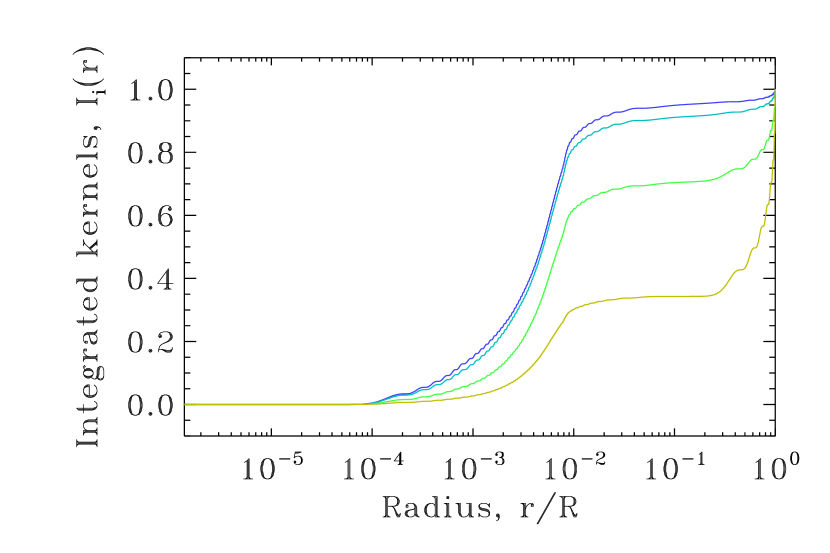
The behaviour in $r=0$ is more complicated. Indeed, one needs to consider the limit of $I_{i}(r)/I_{j}(r)$ in Eq. (10) when $r\rightarrow 0$. Hence, it is useful to know the behaviour of the rotation kernels when $r$ goes to $0$. For $\ell\geq 1$, the vertical and horizontal displacement behave as $\mathcal{O}(r^{\ell-1})$. Therefore, the rotation kernels scale as $r^{2\ell}$ when $r$ goes to $0$ as can be seen from Eq. (3). However, there is one exception to this rule. Indeed, when $r$ goes to $0$, the vertical and horizontal displacements satisfy the relation: $\xi\sim\ell\eta$. If we replace $\xi$ by $\ell\eta$ in Eq. (3), then we obtain the following expression for the numerator:

$$\left(2\ell^{2}-\ell-1\right)\eta^{2}\rho r^{2}=(2\ell+1)(\ell-1)\eta^{2}\rho r^{2}.$$ (11)

This expression is zero when $\ell=1$. Hence, in dipole modes, the lowest order terms cancel out and one needs to consider higher order terms. If we return to expression (3) and substitute $\ell=1$, then the second part of the numerator drops out and we are left with $(\xi-\eta)^{2}\rho r^{2}$. The next order term for $(\xi-\eta)$ behaves as $\mathcal{O}(r^{2})$ since only even powers of $r$ intervene in the displacement functions of dipole modes. When squared and multiplied by $\rho r^{2}$, this leads to an $\mathcal{O}(r^{6})$ behaviour, rather than the $\mathcal{O}(r^{2})$ behaviour initially expected. Finally, if we return to the general case, the integrated kernels will simply behave as $\mathcal{O}(r^{2\ell+1})$, except for dipole modes, for which $I_{i}(r)=\mathcal{O}(r^{7})$. Therefore, when considering the limit $I_{i}(r)/I_{j}(r)$, the modes $i$ and $j$ need to have the same $\ell$ value or else one needs to have $\ell=1$ and and the other $\ell=3$. Otherwise, the limit will either be $0$, thereby leading to $a=0$, or infinite, thereby leading to $b=\infty$.

If we now multiply Eq. (9) by $-\frac{\mathrm{d}\Omega}{\mathrm{d}r}$ and integrate over $[0,R]$, we obtain the following inequalities:

$$a\left[s^{\prime}_{j}-\Omega(R)\right]\leq\left[s^{\prime}_{i}-\Omega(R)\right]\leq b\left[s^{\prime}_{j}-\Omega(R)\right],$$ (12)

where we have made use of the assumption $\frac{\mathrm{d}\Omega}{\mathrm{d}r}<0$, and of Eq. (4), which assumes that $\Omega$ is continuous. Bearing in mind that $a\Omega(R)\leq\Omega(R)\leq b\Omega(R)$, one can simplify the terms proportional to the surface rotation rate, thereby leading us to our final set of inequalities:

$$as^{\prime}_{j}\leq s^{\prime}_{i}\leq bs^{\prime}_{j}.$$ (13)

Although simpler, this last equation is slightly less restrictive than the previous form. Hence, one should use Eq. (12) if the surface rotation rate is known. If the rotation profile, $\Omega$, is discontinuous at $r_{d}$, it is still possible to obtain the inequalities given in Eq. (13), provided that $\Omega(r_{d}^{-})>\Omega(r_{d}^{+})$, which is consistent with $\frac{\mathrm{d}\Omega}{\mathrm{d}r}<0$ as pointed out earlier. As will be discussed in Sect. 2.1.5, observational error bars also need to be taken into account when applying the above inequalities.

We note, in passing, that the quantities $R-r_{i}$ also obey the above inequalities, where $r_{i}=\int_{0}^{R}rK_{i}(r)\mathrm{d}r$. Indeed, an integration by part yields:

$$r_{i}=\int_{0}^{R}rK_{i}(r)\mathrm{d}r=R-\int_{0}^{R}I_{i}(r)\mathrm{d}r.$$ (14)

Hence, integrating Eq. (9) over $[0,R]$ leads to:

$$a(R-r_{j})\leq R-r_{i}\leq b(R-r_{j}).$$ (15)

If $a$ or $b$ is equal to $1$ for a given pair of modes (i.e. if their integrated kernels $I_{i}$ and $I_{j}$ do not cross, as noted above), then the slope of line connecting $(R-r_{i},s^{\prime}_{i})$ to $(R-r_{j},s^{\prime}_{j})$ must be positive. However, it turns out that integrated kernels do cross fairly frequently (as shown in Fig. 3), so one cannot rely on the slope to decide whether a particular pair of modes obey the above inequalities. Instead, one needs to apply the inequalities systematically. We nonetheless expect there to be a general trend in an $(R-r_{i},s^{\prime}_{i})$ diagram, based on these considerations.

Figure 3: Cumulative number of crossings between the $I_{i}(r)$ integrated kernels as a function of position, $r/R$. These crossings were calculated using the $\ell=1$ modes from Model 1, which is introduced in Sect. 3.2.

Bearing in mind that the original goal, as described in the Introduction, is to be able to find rotation profiles which are decreasing and which do not change signs, it is interesting to look at the above problem the other way around and see whether it is possible to construct such rotation profiles for given rotational splittings, assuming they obey the above inequalities. We begin by denoting $\gamma=\frac{s^{\prime}_{i}}{s^{\prime}_{j}}$. The quantity $\gamma$ is between $a$ and $b$ since the rotational splittings satisfy the above inequalities. Furthermore, the function $\frac{I_{i}(r)}{I_{j}(r)}$ ranges from $a$ to $b$, by definition of these constants. If this function is continuous, then there exists a point $r_{\gamma}$ such that $\frac{I_{i}(r_{\gamma})}{I_{j}(r_{\gamma})}=\gamma$. It is then straightforward to see that the following rotation profile reproduces the rotational splittings and satisfies the above constraints:

$$\Omega(r)=\left\{\begin{array}[]{ll}\frac{s^{\prime}_{i}}{I_{i}(r_{\gamma})}&\mbox{ if }0\leq r\leq r_{\gamma}\\ 0&\mbox{ if }r_{\gamma}<r\leq R\end{array}\right..$$ (16)

If the function $\frac{I_{i}(r)}{I_{j}(r)}$ never takes on the value $\gamma$ due to a discontinuity (for instance in a model with a discontinuous density profile), then one could define a rotation profile which is discontinuous at the points $r_{1}$ and $r_{2}$, defined such that $\frac{I_{i}(r_{1})}{I_{j}(r_{1})}\leq\gamma\leq\frac{I_{i}(r_{2})}{I_{j}(r_{2})}$, and solve the relevant system of equations to find by what amount the rotation profile changes at each discontinuity. A more serious difficulty occurs if $r_{\gamma}=0$ and no alternative $r$ values could be used to construct a solution. In such a situation, one can only get arbitrarily close to the solution by setting a discontinuity at $\epsilon$, finding the corresponding rotation profile, then decreasing $\epsilon$. Hence, in summary, the above inequalities provide a necessary and nearly sufficient condition on the rotational splittings of two modes for the existence of a decreasing and positive rotation profile.

Had the above inequalities not provided a nearly sufficient condition for the existence of such profiles, then one would be left wondering if a more stringent set of criteria could be deduced. However, the above results suggest that these are the most restrictive conditions one could find for a given pair of modes. As we will, however, see in a later section, they do not provide the most restrictive conditions for a set of 3 or more modes, as they apply to 2 modes at a time. Also, one must not forget that even if rotational splittings do obey the above inequalities, it does not guarantee that the true rotation profile is indeed decreasing everywhere. Indeed, for any set of rotational splittings, it is always possible to find rotation profiles which have a positive gradient somewhere in the star and/or a sign change.

2.1.2 Inequalities where the centre is excluded

If an upper bound on $-\frac{\mathrm{d}\Omega}{\mathrm{d}r}$ is known in the most central regions of the star, then it is possible to derive slightly different inequalities which exclude these regions and potentially lead to tighter constraints. We start by defining new constants, $a^{\star}$ and $b^{\star}$, as follows:

$$a^{\star}=\min_{r\in[r_{0},R]}\left(\frac{I_{i}(r)}{I_{j}(r)}\right),\qquad b^{\star}=\max_{r\in[r_{0},R]}\left(\frac{I_{i}(r)}{I_{j}(r)}\right).$$ (17)

where $r_{0}$ is the upper bound of the central region under consideration. Hence,

$$\forall r\in[r_{0},R],\qquad a^{\star}I_{j}(r)\leq I_{i}(r)\leq b^{\star}I_{j}(r).$$ (18)

We then multiply this equation by $-\frac{\mathrm{d}\Omega}{\mathrm{d}r}$ and integrate over $[r_{0},R]$. Remembering that

$$-\int_{r_{0}}^{R}\frac{\mathrm{d}\Omega}{\mathrm{d}r}I_{k}(r)\mathrm{d}r=s^{\prime}_{k}-\Omega(R)+\int_{0}^{r_{0}}\frac{\mathrm{d}\Omega}{\mathrm{d}r}I_{k}(r)\mathrm{d}r,$$ (19)

where $k$ corresponds to $i$ or $j$, we finally obtain, after some rearrangement and cancelling out the surface rotation terms:

$$a^{\star}s^{\prime}_{j} + \int_{0}^{r_{0}}\frac{\mathrm{d}\Omega}{\mathrm{d}r}\left[a^{\star}I_{j}(r)-I_{i}(r)\right]\mathrm{d}r\leq s^{\prime}_{i}$$ (20)

$$\leq b^{\star}s^{\prime}_{j}+\int_{0}^{r_{0}}\frac{\mathrm{d}\Omega}{\mathrm{d}r}\left[b^{\star}I_{j}(r)-I_{i}(r)\right]\mathrm{d}r.$$

At this point, we introduce $\mathcal{B}$, the upper bound on $-\frac{\mathrm{d}\Omega}{\mathrm{d}r}$ over the interval $[0,r_{0}]$. The first integral in the above expression can be bounded as follows:

$$-\int_{0}^{r_{0}} \frac{\mathrm{d}\Omega}{\mathrm{d}r} \left[a^{\star}I_{j}(r)-I_{i}(r)\right]\mathrm{d}r$$ (21)

$$\leq -\int_{0}^{r_{0}}\frac{\mathrm{d}\Omega}{\mathrm{d}r}\max\left[0,a^{\star}I_{j}(r)-I_{i}(r)\right]\mathrm{d}r$$

$$\leq \mathcal{B}\int_{0}^{r_{0}}\max\left[0,a^{\star}I_{j}(r)-I_{i}(r)\right]\mathrm{d}r,$$

where we have also made use of the assumption $\frac{\mathrm{d}\Omega}{\mathrm{d}r}\leq 0$ over the interval $[0,r_{0}]$. We note that, if we substitute $a$ for $a^{\star}$, then $\max\left[0,aI_{j}(r)-I_{i}(r)\right]$ is always zero, thereby cancelling out the right-hand side. The integral term would then drop out of Eq. (20). A similar manipulation with the second integral term leads to:

$$\int_{0}^{r_{0}} \frac{\mathrm{d}\Omega}{\mathrm{d}r} \left[b^{\star}I_{j}(r)-I_{i}(r)\right]\mathrm{d}r$$ (22)

$$\leq \mathcal{B}\int_{0}^{r_{0}}\max\left[0,I_{i}(r)-b^{\star}I_{j}(r)\right]\mathrm{d}r.$$

Once more, if we substitute $b$ for $b^{\star}$, the right-had side cancels out. When substituted into Eq. (20), these inequalities lead to:

$$a^{\star}s^{\prime}_{j} - \mathcal{B}\int_{0}^{r_{0}}\max\left[0,a^{\star}I_{j}(r)-I_{i}(r)\right]\mathrm{d}r\leq s^{\prime}_{i}$$ (23)

$$\leq b^{\star}s^{\prime}_{j}+\mathcal{B}\int_{0}^{r_{0}}\max\left[0,I_{i}(r)-b^{\star}I_{j}(r)\right]\mathrm{d}r.$$

The advantage of this equation over Eq. (13) is that the constants $a^{\star}$ and $b^{\star}$ may be much more constraining than $a$ and $b$, given that the latter may be overly affected by the very inner regions. In particular, this would allow comparisons between splittings for different $\ell$ values, for which the constants $a$ or $b$ could be $0$ or infinite, respectively. The drawback is trying to find an appropriate value for $\mathcal{B}$. One can expect $\mathcal{B}$ to become small in the central regions since $\frac{\mathrm{d}\Omega}{\mathrm{d}r}=\mathcal{O}(r)$.

In much the same way as was done above, one can check to see if the above inequalities provide a sufficient condition for obtaining a positive, decreasing rotation profile, subject to the supplementary condition $-\frac{\mathrm{d}\Omega}{\mathrm{d}r}\leq\mathcal{B}$ over the interval $0\leq r<r_{0}$. If $\frac{\mathrm{d}\Omega}{\mathrm{d}r}$ is prescribed over the interval $[0,r_{0}[$, one could apply a similar approach to what was done above and attempt to define a radial coordinate $r_{\gamma^{\star}}$ such that such that $\gamma^{\star}=\frac{s^{\prime}_{i}+\int_{0}^{r_{0}}\frac{\mathrm{d}\Omega}{\mathrm{d}r}I_{i}(r)\mathrm{d}r}{s^{\prime}_{j}+\int_{0}^{r_{0}}\frac{\mathrm{d}\Omega}{\mathrm{d}r}I_{j}(r)\mathrm{d}r}=\frac{I_{i}(r_{\gamma^{\star}})}{I_{j}(r_{\gamma^{\star}})}$. If such a point exists, then it is possible to construct a rotation profile which is decreasing and satisfies the rotational splittings. However, Eq. (23) does not guarantee that $\gamma^{\star}$ is between $a^{\star}$ and $b^{\star}$, and hence that $r_{\gamma^{\star}}$ exists. Only Eq. (20) provides such a guarantee. One may try to adjust the function $\frac{\mathrm{d}\Omega}{\mathrm{d}r}$ over the interval $[0,r_{0}[$, but would only succeed in enforcing either $a^{\star}\leq\gamma^{\star}$ or $\gamma^{\star}\leq b^{\star}$. One could then take on a different approach, and define the points $r_{a^{\star}}$ and $r_{b^{\star}}$ such that $\frac{I_{i}(r_{a^{\star}})}{I_{j}(r_{a^{\star}})}=a^{\star}$ and $\frac{I_{i}(r_{b^{\star}})}{I_{j}(r_{b^{\star}})}=b^{\star}$. As opposed to $r_{\gamma^{\star}}$, these points are guaranteed to exist. However, as described in Appendix A, if one defines a rotation profile with discontinuities at those points, and which reproduces the rotational splittings, only Eq. (20) guarantees that the rotation profile will decrease across these discontinuities. Hence, only Eq. (20) provides a necessary and sufficient condition for the rotation splittings to correspond to a positive decreasing rotation profile, provided it is decreasing over the interval $[0,r_{0}[$. Equation (23), in contrast, constitutes a necessary but insufficient condition on the rotational splittings.

2.1.3 Three or more modes

So far, we have only considered two modes in isolation. However, in typical stars, a larger number of rotational splittings are observed. Of course, one can always apply the above inequalities to every pair of rotational splittings. However, it is obvious that a more complicated strategy than what was described in the previous section is needed in order to construct a rotation profile which satisfies all of the rotational splittings simultaneously, and yet still has a negative gradient throughout the star. Indeed, certain properties of the rotation profile only emerge when a sufficient number of rotational splittings are used together. Hence, in what follows, we briefly explore a way of generalising the above inequalities to more than two modes. Let us consider an inequality of the following form:

$$\forall r\in[0,R],\,\,\,\,\sum_{i}a_{i}I_{i}(r)\leq\sum_{j}b_{j}I_{j}(r),$$ (24)

where we are assuming that the $a_{i}$ and $b_{j}$ are positive. Then using the same methodology as above, we deduce the following inequalities on the corresponding rotational splittings:

$$\sum_{i}a_{i}s^{\prime}_{i}\leq\sum_{j}b_{j}s^{\prime}_{j}.$$ (25)

We note that it was possible to remove the surface rotation rate because $\sum_{i}a_{i}\leq\sum_{j}b_{j}$ (as deduced from Eq. (24) for $r=R$). If one excludes the central region, $[0,r_{0}]$, then the following inequality is obtained:

$$\sum_{i}a_{i}s^{\prime}_{i}-\mathcal{B}\int_{0}^{r_{0}}\max\left[0,\sum_{i}a_{i}I_{i}(r)-\sum_{j}b_{j}I_{j}(r)\right]\mathrm{d}r\leq\sum_{j}b_{j}s^{\prime}_{j},$$ (26)

where $\mathcal{B}$ is an upper bound on $-\frac{\mathrm{d}\Omega}{\mathrm{d}r}$ over the interval $[0,r_{0}]$. One can also obtain the following condition by making use of the inequalities $\int_{0}^{r_{0}}\frac{\mathrm{d}\Omega}{\mathrm{d}r}I_{j}(r)\mathrm{d}r\leq 0$, thereby allowing us to remove these terms altogether:

$$\sum_{i}a_{i}\left(s^{\prime}_{i}-\mathcal{B}\int_{0}^{r_{0}}I_{i}(r)\mathrm{d}r\right)\leq\sum_{j}b_{j}s^{\prime}_{j}.$$ (27)

Although less restrictive than Eq. (26), this latter inequality has the advantage of being linear with respect to the coefficients $a_{i}$ and $b_{j}$.

The main difficulty in the above inequalities is finding the constants $a_{i}$ and $b_{j}$ in such a way as to provide tight constraints. For instance, one could choose a set of $b_{j}$ values, and search for $a_{i}$ values which maximise the left hand side of Eqs. (25) or (26) while respecting Eq. (24). Equation (24) could be applied at each mesh point, thereby providing a set of $N$ linear inequalities on the coefficients $a_{i}$, where $N$ is the number of mesh points. Maximising the left-hand side of Eq. (25) would then require methods from linear programming such as the simplex algorithm. A similar strategy can also be applied to Eq. (27). In contrast, maximising the left-hand side of Eq. (26) would require a method from mathematical optimisation, due to its non-linear form. In the next section, we carry out a comparison between these inequalities and inverse methods, thereby providing further insights into how to choose the coefficients $a_{i}$ and $b_{j}$.

2.1.4 Link with inverse methods

In order to understand the link between the above inequalities and inverse methods, we start with Eq. (24) and subtract $\sum_{i}a_{i}I_{i}(r)$ from both sides:

$$\forall r\in[0,R],\,\,\,\,0\leq\sum_{j}b_{j}I_{j}(r)-\sum_{i}a_{i}I_{i}(r)\equiv\mathcal{K}(r).$$ (28)

The right-hand side of this inequality is a linear combination of kernels that plays exactly the same role as an averaging kernel in inverse methods. There is, however, one key difference: $\mathcal{K}(r)$ needs to be positive everywhere, as indicated by the equation, in order for the inequality to carry through the integration onto the rotational splittings. In contrast, the averaging kernels from inverse methods are not obtained with such a goal in mind, and therefore frequently take on negative values.

This condition can be relaxed if one excludes the centre, or some other region(s) in the star. Indeed, in such a situation, the combined kernel, $\mathcal{K}$, only needs to be positive in those regions which have not been excluded. The upper bound on $-\frac{\mathrm{d}\Omega}{\mathrm{d}r}$ can then be used to constrain the supplementary terms which arise from the excluded regions, as is done, for instance, in Eq. (26). Hence, one could, in principle, take a set of inversion coefficients, exclude the regions where the averaging kernel is negative, and deduce inequalities on the rotational splittings for a given upper bound, $\mathcal{B}$. Conversely, one could search for the limiting value of $\mathcal{B}$ beyond which the inequalities break down. If the averaging kernel is well localised, one will have primarily tested whether the rotation gradient is negative in that particular region. This approach could also be combined with a simplex method, as described above, in order to find tighter constraints on the splittings.

2.1.5 Error bars

In practise, it will be necessary to take into account error bars on observed rotational splittings. As will be described in this section, this introduces complications when interpreting the above inequalities. Indeed, if one of the inequalities is not satisfied, one can only deduce that the rotation profile has a positive gradient with some probability that needs to be determined. In order to illustrate this, we start with Eq. (25) as a generic form for the inequalities, group the non-zero terms together on the left-hand side, and introduce error terms:

$$\underbrace{\sum_{i}a_{i}s^{\prime}_{i}-\sum_{j}b_{j}s^{\prime}_{j}}_{s^{\prime}}+\underbrace{\sum_{i}a_{i}\varepsilon^{\prime}_{i}-\sum_{j}b_{j}\varepsilon^{\prime}_{j}}_{\varepsilon^{\prime}}\leq 0,$$ (29)

where $\varepsilon^{\prime}_{i}$ is the error realisation on a given normalised splitting, $s^{\prime}$ represents the combined splittings, and $\varepsilon^{\prime}$ the combined errors. For a true violation of the inequality, one needs $s^{\prime}>0$. However, since only the measurement $s^{\prime}+\varepsilon^{\prime}$ is available, one has to evaluate the probability that $s^{\prime}+\varepsilon^{\prime}>\varepsilon^{\prime}$. An obvious approach is to compare the $1\sigma$ error bar on $\varepsilon^{\prime}$, which we will denote $\sigma^{\prime}$, with the measurement. This can be obtained as a quadratic sum of the individual $1\sigma$ error bars:

$$\sigma^{\prime}=\sqrt{\sum_{i}a_{i}^{2}(\sigma^{\prime}_{i})^{2}+\sum_{j}b_{j}^{2}(\sigma^{\prime}_{j})^{2}},$$ (30)

where the $\sigma^{\prime}_{i}$ are the $1\sigma$ error bars on the individual normalised splittings. Hence, if $s^{\prime}+\varepsilon^{\prime}$ is equal to $3\sigma^{\prime}$, and $\varepsilon^{\prime}$ follows a normal distribution, the probability that the inequality is violated is $99.87\,\%$ (where we’ve taken into account the fact that there is violation in only one of wings of the distribution for $\varepsilon^{\prime}$). It would be tempting to conclude that this is the probability that the rotation profile has a positive gradient. However, one will typically test a large number of inequalities which increases the chances of finding large deviations on one of the $\varepsilon^{\prime}$ values and hence of having a false alarm. Given the correlations between the different inequalities, it is not straightforward how to calculate the probability of a false alarm. As will be described in Sect. 3, we will carry out Monte-Carlo simulations to estimate such a probability.

2.2 Rotation profiles subject to Rayleigh’s stability criterion

2.2.1 Inequalities for the full domain

A different set of inequalities can be obtained from Rayleigh’s stability criterion. According to this criterion, the angular momentum must increase with the distance to the rotation axis: otherwise, the fluid will be dynamically unstable and can free up energy by redistributing its angular momentum (e.g. Rieutord, 1997). Mathematically, this is expressed by the condition:

$$\frac{\partial(\varpi^{4}\Omega^{2})}{\partial\varpi}>0,$$ (31)

where $\varpi$ is the distance to the rotation axis. If we furthermore assume that the rotation profile only depends on $r$, this criterion then becomes:

$$\frac{\mathrm{d}(r^{4}\Omega^{2})}{\mathrm{d}r}>0,\qquad\mbox{{i.e.}}\qquad\frac{\mathrm{d}\ln|\Omega|}{\mathrm{d}\ln r}>-2.$$ (32)

Hence, this criterion gives the maximum rate at which a rotation profile can decrease before the fluid becomes unstable. We note that such a criterion is incompatible with a sign change in the rotation profile, except at discontinuities. However, in realistic stars, viscosity, even though it is small, would remove true discontinuities, thereby suppressing sign changes. If a discontinuity were present in the rotation profile, it would be stable only if the absolute value of the rotation rate increases outward across the discontinuity, which is the opposite from what was considered in the previous section (if we ignore sign changes). Finally, in real stars, this criterion is only one of the terms in the more general Solberg-Hoiland criterion for convective stability (e.g. Maeder, 2009). Hence there could be situations where an unstable rotation profile is stabilised by, say, a $\mu$ gradient.

At this point, we will assume that the rotation profile does not change signs. Accordingly, we will see the consequences of the inequality $\frac{\mathrm{d}(r^{2}\Omega)}{\mathrm{d}r}>0$ rather than those of Eq. (32). In order to derive inequalities on the rotational splittings, we start from Eq. (1), do an integration by part, and divide both sides by $\int_{0}^{R}\frac{K_{i}(r)}{r^{2}}\mathrm{d}r$:

$$\frac{s_{i}}{\left(1-C_{i}\right)\int_{0}^{R}\frac{K_{i}(r)}{r^{2}}\mathrm{d}r}=R^{2}\Omega(R)-\int_{0}^{R}\frac{\mathrm{d}(r^{2}\Omega)}{\mathrm{d}r}\left[\frac{\int_{0}^{r}\frac{K_{i}(r^{\prime})}{(r^{\prime})^{2}}\mathrm{d}r^{\prime}}{\int_{0}^{R}\frac{K_{i}(r^{\prime})}{(r^{\prime})^{2}}\mathrm{d}r^{\prime}}\right]\mathrm{d}r.$$ (33)

If a discontinuity is present, for instance at $r=r_{d}$, one would obtain the following formula:

$$\frac{s_{i}}{\left(1-C_{i}\right)\int_{0}^{R}\frac{K_{i}(r)}{r^{2}}\mathrm{d}r} = R^{2}\Omega(R)+r_{d}^{2}\left[\Omega(r_{d}^{-})-\Omega(r_{d}^{+})\right]\frac{\int_{0}^{r_{d}}\frac{K_{i}(r)}{r^{2}}\mathrm{d}r}{\int_{0}^{R}\frac{K_{i}(r)}{r^{2}}\mathrm{d}r}$$ (34)

$$-\int_{0}^{r_{d}}\frac{\mathrm{d}(r^{2}\Omega)}{\mathrm{d}r}\left[\frac{\int_{0}^{r}\frac{K_{i}(r^{\prime})}{(r^{\prime})^{2}}\mathrm{d}r^{\prime}}{\int_{0}^{R}\frac{K_{i}(r^{\prime})}{(r^{\prime})^{2}}\mathrm{d}r^{\prime}}\right]\mathrm{d}r$$

$$-\int_{r_{d}}^{R}\frac{\mathrm{d}(r^{2}\Omega)}{\mathrm{d}r}\left[\frac{\int_{0}^{r}\frac{K_{i}(r^{\prime})}{(r^{\prime})^{2}}\mathrm{d}r^{\prime}}{\int_{0}^{R}\frac{K_{i}(r^{\prime})}{(r^{\prime})^{2}}\mathrm{d}r^{\prime}}\right]\mathrm{d}r.$$

Of course, the difference $\Omega(r_{d}^{-})-\Omega(r_{d}^{+})$ would have to be negative, in keeping with Rayleigh’s criterion. We note, in passing, that the rotation kernels, $K_{i}$, behave as $r^{n}$ in the centre, where $n\geq 4$. Hence the ratio, $K_{i}(r)/r^{2}$ always goes to zero in the centre. From now on, we will use the following notation to designate a second type of normalised rotational splitting:

$$\tilde{s}_{i}\equiv\frac{s_{i}}{\left(1-C_{i}\right)\int_{0}^{R}\frac{K_{i}(r)}{r^{2}}\mathrm{d}r}.$$ (35)

A first inequality can be found straight away, in much the same way as was done above. The second term on the right-hand side of Eq. (33) is negative, given the assumption $\frac{\mathrm{d}(r^{2}\Omega)}{\mathrm{d}r}>0$. This leads to the following inequality:

$$\tilde{s}_{i}<R^{2}\Omega(R).$$ (36)

This inequality sets a lower limit on the surface rotation rate based on the internal rotation rate, as measured by the rotational splitting. This is consistent with Rayleigh’s criterion which gives the maximum rate at which the rotation profile can decrease.

We then introduce a second type of integrated kernel:

$$J_{i}(r)\equiv\frac{\int_{0}^{r}\frac{K_{i}(r^{\prime})}{(r^{\prime})^{2}}\mathrm{d}r^{\prime}}{\int_{0}^{R}\frac{K_{i}(r)}{r^{2}}\mathrm{d}r}.$$ (37)

Examples of this type of integrated kernel are shown in Fig. 4.

Figure 4: (colour online) Second type of integrated normalised kernels for the same modes as in Fig. 1 (the same colour scheme is used in both figures). These integrated kernels are very similar, so it is difficult to distinguish them, even though there’s a mixture of p-like and g-like modes.

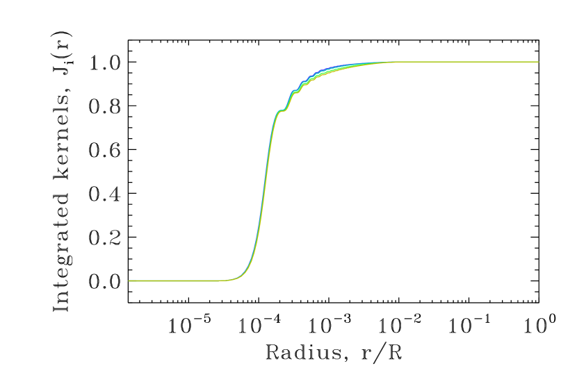
As was done above, we find, for a given pair of modes $(i,j)$, inequalities of the following form:

$$\forall r\in[0,R],\qquad\tilde{a}J_{j}(r)\leq J_{i}(r)\leq\tilde{b}J_{j}(r),$$ (38)

where

$$\tilde{a}=\min_{r\in[0,R]}\left(\frac{J_{i}(r)}{J_{j}(r)}\right),\qquad\tilde{b}=\max_{r\in[0,R]}\left(\frac{J_{i}(r)}{J_{j}(r)}\right).$$ (39)

Figure 5 illustrates ratios of the second type of integrated kernels, from which we can determine $\tilde{a}$ and $\tilde{b}$. Once more, we obtain the relations $\tilde{a}\leq 1\leq\tilde{b}$ by inserting $r=1$ into Eq. (38). In order to avoid having $\tilde{a}=0$ or $\tilde{b}=\infty$, the integrated kernels $J_{i}$ and $J_{j}$ need to have the same behaviour in the centre. Hence, the $\ell$ values of modes $i$ and $j$, should be the same or should be $1$ and $3$.

Figure 5: Ratios of second type of integrated kernels for the same pairs of modes as in Fig. 2.

We then multiply Eq. (38) by $-\frac{\mathrm{d}(r^{2}\Omega)}{\mathrm{d}r}$ and integrate over the interval $[0,R]$. This yields, taking into account the sign change:

$$\tilde{a}\left[\tilde{s}_{j}-\Omega(R)R^{2}\right]\geq\left[\tilde{s}_{i}-\Omega(R)R^{2}\right]\geq\tilde{b}\left[\tilde{s}_{j}-\Omega(R)R^{2}\right],$$ (40)

where we have made use of Eq. (33). This time, given the inverted inequalities, the surface terms cannot simply be cancelled out and must therefore be kept. Furthermore, because of the inequality given in Eq. (36), the terms in Eq. (40) are negative. Hence, we rearrange this inequality so as to make positive terms appear, thereby leading us to our final form:

$$\tilde{b}\tilde{s}_{j}-(\tilde{b}-1)\Omega(R)R^{2}\leq\tilde{s}_{i}\leq\tilde{a}\tilde{s}_{j}+(1-\tilde{a})\Omega(R)R^{2},$$ (41)

where $\delta\tilde{s}_{j}$ is the error bar on the normalised splitting, $\tilde{s}_{j}$. Had we worked with a discontinuous profile, the same inequalities would be obtained, as long as the rotation rate increases across the discontinuities (which is the opposite to what we assumed in the previous section). Otherwise, supplementary terms for each discontinuity where the rotation rate decreases would need to be included, but again we emphasise that such discontinuities would not satisfy Rayleigh’s stability criterion.

In analogy with what was done above, we introduce the quantity $\tilde{r}_{i}$, defined as follows:

$$\tilde{r}_{i}=\frac{\int_{0}^{R}r\frac{K_{i}(r)}{r^{2}}\mathrm{d}r}{\int_{0}^{R}\frac{K_{i}(r)}{r^{2}}\mathrm{d}r}.$$ (42)

Carrying out an integration by parts leads to the following equality:

$$\tilde{r}_{i}=R-\int_{0}^{R}J_{i}(r)\mathrm{d}r.$$ (43)

Combining Eq. (43) with the inequalities in Eq. (38) then yields:

$$\tilde{a}(R-\tilde{r}_{j})\leq R-\tilde{r}_{i}\leq\tilde{b}(R-\tilde{r}_{j}).$$ (44)

Hence, the quantities $R-\tilde{r}_{i}$ obey the opposite inequalities to the normalised splittings $\tilde{s}_{i}$. Accordingly, if $\tilde{a}=1$ or $\tilde{b}=1$ (i.e. if the integrated kernels $J_{i}(r)$ and $J_{j}(r)$ do not cross), then the slope of the line connecting $(R-\tilde{r}_{i},\tilde{s}_{i})$ to $(R-\tilde{r}_{j},\tilde{s}_{j})$ is negative. However, the integrated kernels do cross frequently, as illustrated in Fig. 6, so one should instead look at the general trend in an $(R-\tilde{r}_{i},\tilde{s}_{i})$ diagram. Only a systematic application of the inequalities will yield conclusive results.

Figure 6: Cumulative number of crossings of between the $J_{i}(r)$ integrated kernels as a function of position, $r/R$. These crossings were calculated using the $\ell=1$ modes from Model 1, which is introduced in Sect. 3.2.

One can then try to see if the above conditions are sufficient for the existence of a rotation profile which satisfies Rayleigh’s criterion. This time, in keeping with the inequalities, we must assume the surface rotation rate is imposed. As was done previously, we introduce the ratio $\tilde{\gamma}=\frac{R^{2}\Omega(R)-\tilde{s}_{i}}{R^{2}\Omega(R)-\tilde{s}_{j}}$ and its corresponding radial coordinate, $r_{\tilde{\gamma}}$, defined such that $\tilde{\gamma}=\frac{J_{i}(r_{\tilde{\gamma}})}{J_{j}(r_{\tilde{\gamma}})}$. This radial coordinate is guaranteed to exist provided the function $\frac{J_{i}(r)}{J_{j}(r)}$ is continuous. We then define a rotation profile which is discontinuous at $r_{\tilde{\gamma}}$ and where $\frac{\mathrm{d}(r^{2}\Omega)}{\mathrm{d}r}=0$ everywhere else:

$$\Omega(r)=\left\{\begin{array}[]{ll}\frac{\mu}{r^{2}}&\mbox{ if }0\leq r\leq r_{\tilde{\gamma}}\\ \frac{\mu+\lambda}{r^{2}}&\mbox{ if }r_{\tilde{\gamma}}<r\leq R\end{array}\right..$$ (45)

The constants $\mu$ and $\lambda$ are obtained by imposing the correct surface rotation rate and rotational splittings. This leads to:

$$\lambda=\frac{R^{2}\Omega(R)-\tilde{s}_{i}}{J_{i}(r_{\tilde{\gamma}})},\qquad\mu=R^{2}\Omega(R)-\frac{R^{2}\Omega(R)-\tilde{s}_{i}}{J_{i}(r_{\tilde{\gamma}})}.$$ (46)

It is straightforward to show that $\lambda$ is positive, using Eq. (36). However, it is not clear whether $\mu$ is positive or not, meaning the above rotation profile might be negative in the centre. Also, we were not able to show that $|\mu|<|\mu+\lambda|$ which is needed to ensure that the absolute value of $\Omega$ increases across the discontinuity, and hence that Rayleigh’s criterion is verified. Instead, the above rotation profile only satisfies the criterion $\frac{\mathrm{d}(r^{2}\Omega)}{\mathrm{d}r}\geq 0$, which is slightly less restrictive than the condition we obtained when we assumed the rotation profile doesn’t change signs in addition to Rayleigh’s criterion. Accordingly, if $\mu$ is positive, then $|\mu|\leq|\mu+\lambda|$ and Rayleigh’s criterion is nearly satisfied (i.e. $\frac{\mathrm{d}(r^{4}\Omega^{2})}{\mathrm{d}r}\geq 0$). Hence, this simple strategy is unable to produce a fool-proof solution solely based on the above inequalities and seems to indicate that these do not provide a sufficient, or nearly sufficient, condition for the existence of a rotation profile which satisfies Rayleigh’s criterion.

2.2.2 Inequalities where the centre is excluded

If an upper bound on $\frac{\mathrm{d}(r^{2}\Omega)}{\mathrm{d}r}$ in the central regions is known, then it is possible to derive some slightly different inequalities, much like in the previous section. We begin by introducing the quantities $\tilde{a}^{\star}$ and $\tilde{b}^{\star}$:

$$\tilde{a}^{\star}=\min_{r\in[r_{0},R]}\left(\frac{J_{i}(r)}{J_{j}(r)}\right),\qquad\tilde{b}^{\star}=\max_{r\in[r_{0},R]}\left(\frac{J_{i}(r)}{J_{j}(r)}\right).$$ (47)

Then, following a similar reasoning as in the previous section, we finally obtain:

$$\tilde{b}^{\star} \tilde{s}_{j}-(\tilde{b}^{\star}\!-\!1)\Omega(R)R^{2}-\tilde{\mathcal{B}}\!\!\int_{0}^{r_{0}}\!\!\!\!\!\max\left[0,J_{i}(r)-\tilde{b}^{\star}J_{j}(r)\right]\mathrm{d}r$$ (48)

$$\leq \tilde{s}_{i}$$

$$\leq \tilde{a}^{\star}\tilde{s}_{j}+(1-\tilde{a}^{\star})\Omega(R)R^{2}+\tilde{\mathcal{B}}\!\!\int_{0}^{r_{0}}\!\!\!\!\!\max\left[0,\tilde{a}^{\star}J_{j}(r)-J_{i}(r)\right]\mathrm{d}r,$$

where $\tilde{\mathcal{B}}$ denotes the upper bound on $\frac{\mathrm{d}(r^{2}\Omega)}{\mathrm{d}r}$ over the interval $[0,r_{0}]$. We do note that to first order, $\frac{\mathrm{d}(r^{2}\Omega)}{\mathrm{d}r}$ behaves as $2r\Omega$ in the centre.

3 Applications

3.1 Direct application of the inequalities

A natural and straightforward application of the above inequalities is to see whether the rotation profile of a given star has a positive gradient and/or fails to respect Rayleigh’s criterion. In what follows, we will therefore test these inequalities in artificial situations to see how effective they are.

We start by using Model S (Christensen-Dalsgaard et al., 1996) and impose the following rotation profile:

$$\Omega(x)=A+B\tanh\left(\frac{x-x_{0}}{d}\right)-C\tanh\left(\frac{x-x_{1}}{d}\right),$$ (49)

where $A=B=1.25$, $C=1.5$, $x_{0}=0.220$, $x_{1}=0.432$, and $d=0.05$. This rotation profile and its derivatives are displayed in the upper panel of Fig. 7. As can be seen, it has a positive gradient in the first $33\%$ of the star, and does not satisfy Rayleigh’s criterion over a narrow region around $0.45\,R$. We then considered a set of $44$ modes with harmonic degrees $\ell=1-3$ from which we calculated “observed” rotational splittings. We assumed these splittings follow a normal distribution, and their $1\sigma$ error bars are $0.0067\,\mu$Hz, which is somewhat smaller than what is achieved with the Kepler satellite.

Figure 7: (Colour online) (Upper panel) Rotation profile and associated derivatives used in first test case on Model S. (Middle panel) Combined kernel from simplex method which led to a detection of a positive gradient. (Bottom panel) SOLA inversion results on $\frac{\mathrm{d}\Omega}{\mathrm{d}x}$ along with $1\sigma$ error bars.

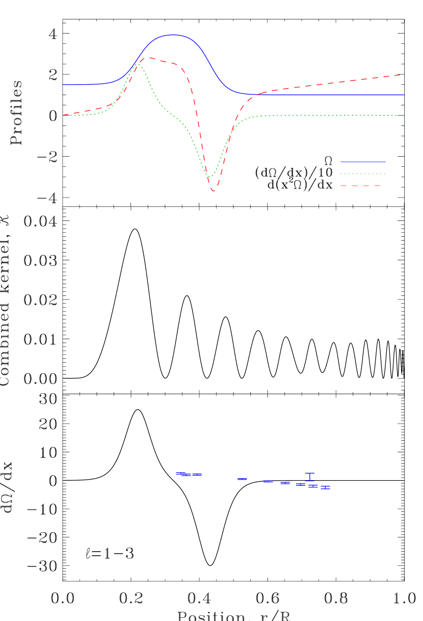
A systematic application of the inequalities (13) and (23) to all pairs of modes with degrees $\ell=1$ to $3$ did not reveal a negative gradient. However, using Eq. (25), we were able to place tighter constraints on the splittings. We systematically applied this equation, in which each splitting was isolated to one side, then the other, of the inequality, and a simplex algorithm used to optimise the coefficients of the remaining splittings. This approach allowed us to deduce lower and upper bounds on each splitting, and to show that the rotational splitting of the $\ell=3$ mode with the lowest radial order ($n=13$) is approximately $4.99\sigma$ beyond the bound predicted by Eq. (25), i.e. we showed that $s^{\prime}/\sigma^{\prime}=4.99$. A naive interpretation of this would lead to the conclusion that the probability of a false alarm is $3.0\times 10^{-7}$. However, as discussed in Sect. 2.1.5, this does not take into account the fact that we are testing multiple inequalities, which increases the probability of having a large deviation on one of them. We therefore carried out a Monte Carlo test with $10^{6}$ realisations of the splittings. We calculated the maximal value of $\varepsilon^{\prime}/\sigma^{\prime}$ for each realisation, using the coefficients from the inequalities based on the mode pairs and based on the simplex approach, and counted the number of times the threshold $4.99$ was exceeded. This occurred in 166 cases, thereby implying a probability of $1.7\times 10^{-4}$ for a false alarm, i.e. substantially larger than the above value. A similar test, using splittings from a decreasing profile, yielded a probability of $1.5\times 10^{-4}$, thereby showing the result is robust. Even then, this new value is likely to be an underestimate, because the Monte Carlo simulation was carried out for fixed coefficients. Ideally, one would want to repeat the simplex calculation for each realisation of the splittings, since the results are optimised for the given set of splittings. However, the numerical cost of such an approach is too high to obtain a result in a reasonable amount of time.

Figure 8: (Colour online) Rotational splittings and $1\sigma$ error bars (solid red lines), constraints deduced from inequalities on pairs of modes (dotted blue lines), and constraints from multiple modes using simplex method (dashed green lines). The lighter lines denote the $1\sigma$ error bars. Right panel: zoom on $\ell=3$ mode where an inequality breaks down by $4.99\sigma$ (as indicated by the arrow).

The reason why the inequality failed for the $\ell=3$ mode is straightforward to understand. The middle panel of Fig. 7 shows the resultant combined kernel, $\mathcal{K}$. This kernel has a maximum amplitude where the rotation profile increases sharply and a low amplitude near the sharp decrease. Hence, the integral of the product $-\frac{\mathrm{d}\Omega}{\mathrm{d}r}\mathcal{K}$ is negative which leads to a break-down of the inequalities for sufficiently small error bars. The lower panel of Fig. 7 shows the results obtained from a SOLA inversion of $\frac{\mathrm{d}\Omega}{\mathrm{d}x}$. Given that only the $\ell=1$ to $3$ modes were used, the averaging kernels are poorly localised and the resultant inverted profile a poor match to $\frac{\mathrm{d}\Omega}{\mathrm{d}x}$, which inspires little confidence in the inversion. Nonetheless, the inversion does detect a positive gradient with a $2.87\sigma$ margin. Hence, the above inequalities, in conjunction with the simplex method, have yielded firmer results than the inversion.

In contrast to the tests based on finding a positive gradient, those based on Rayleigh’s criterion failed to detect a decrease in the angular momentum. Possible explanations for this failure is that the region with this decrease is either too narrow, or poorly located, given the set of modes we considered.

We also considered a second rotation profile with model S:

$$\Omega(x)=\frac{A}{1+\left(\frac{x}{C}\right)^{2}}+\frac{B}{1+\left(\frac{x^{2}-D^{2}}{E^{2}}\right)^{2}}$$ (50)

where $x=r/R$, $A=1\,\mu$Hz, $B=0.5\,\mu$Hz, $C=0.3$, $D=0.4$, and $E=0.2$. This rotation profile has been designed to have a positive gradient in a localised region, fail Rayleigh’s criterion in another region, and have a zero derivative in the centre, as expected from regularity conditions. Figure 9 illustrates this rotation profile, as well as $\mathrm{d}\Omega/\mathrm{d}x$ and $\mathrm{d}(x^{2}\Omega)/\mathrm{d}x$.

Figure 9: (Colour online) The rotation profile, as based on Eq. (50), and its derivatives.

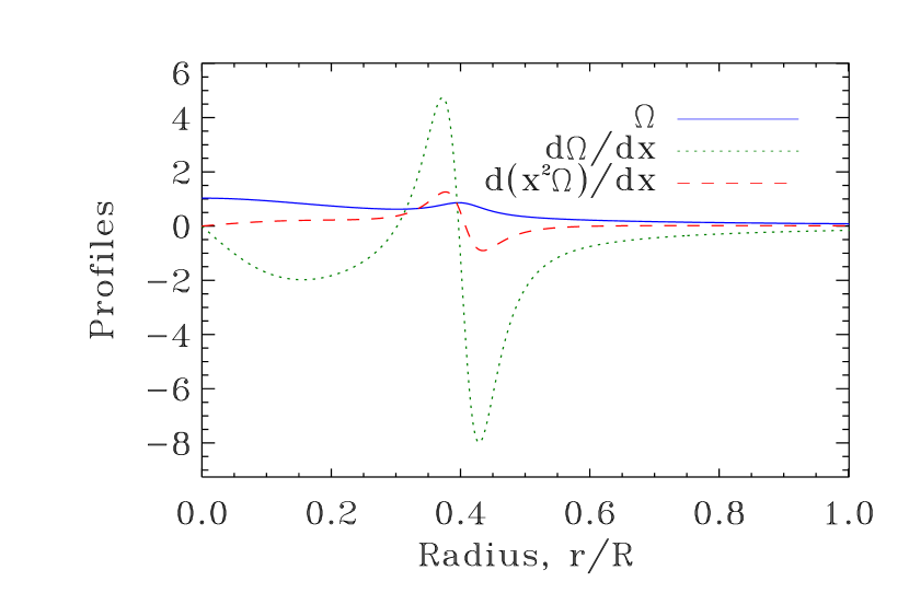
A set of $282$ modes with $\ell$ ranging from $1$ to $20$ were calculated using the ADIPLS pulsation code (Christensen-Dalsgaard, 2008). Such an extensive set is naturally out of reach for stars other than the sun, given cancellation effects, but is what is needed to carry out a sufficiently detailed inversion of the rotation profile. Rotational splittings were calculated using the above profile, and their $1\sigma$ bars were set to $0.0033\,\mu$Hz, which is smaller than what is currently achieved with the Kepler mission.

Figure 10 shows the result of a SOLA inversion (Pijpers & Thompson, 1992, 1994) of the gradient of the rotation profile. The $1\sigma$ error bars are displayed in this plot. The positive gradient shows up clearly.

Figure 10: (Colour online) Inverted rotation profile gradient. The continuous line shows the actual rotation profile gradient, whereas the blue crosses indicate inversion results and associated $1\sigma$ error bars.

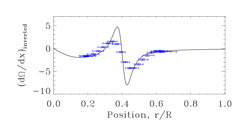
In contrast to the inversions, a systematic application of the inequalities (13) and (23) to all pairs of modes did not reveal a positive gradient. The same also applied to tests based on multiple modes, as described above (we limited ourselves to modes with $\ell=1$ to $10$, given the numerical cost of the simplex algorithm). We also applied a heuristic approach which consisted in recuperating the inversion coefficients and adjusting them so as to have a positive combined kernel everywhere. This strategy was to no avail even if the error bars were set to nearly 0. A possible explanation for these failures is the fact that the rotation profile decreases only over a very narrow region.

One may also see whether it is possible to show that the underlying profile does not satisfy Rayleigh’s criterion. Figure 11 shows inversion results for the gradient of the angular momentum, using the integrated kernels defined in Eq. (37). As can be seen for the full set of modes (upper panel), the inversion is able to detect the region which does not satisfy Rayleigh’s criterion.

Figure 11: (Colour online) Inverted profile for the gradient of the angular momentum, using $\ell=1$ to $20$ modes (upper panel) and only $\ell=8$ modes (lower panel). The continuous line shows the actual gradient, whereas the blue crosses indicate inversion results and associated $1\sigma$ error bars. For the sake of clarity, the horizontal error bars (obtained from the averaging kernels) have been omitted in the lower panel.

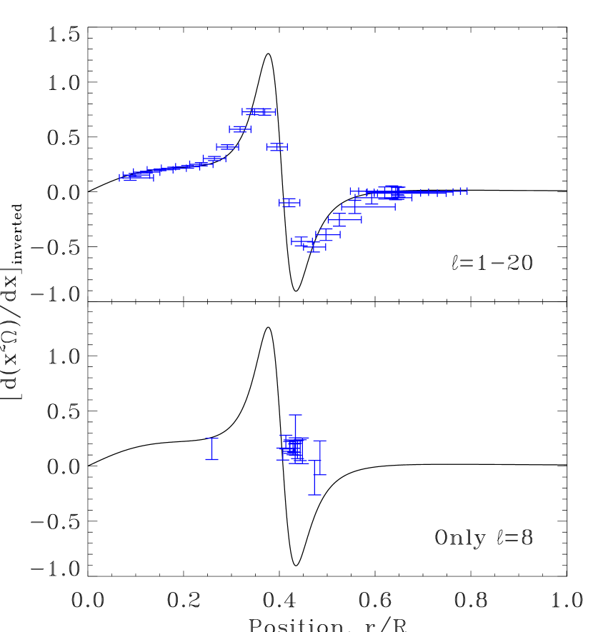
We then systematically applied the inequalities (41) for each pair of modes. Figure 12 shows the maximal values of $\varepsilon^{\prime}/\sigma^{\prime}$ as a function of the harmonic degree. Three different cases are investigated. The solid line shows what happens if we use the exact surface rotation rate, $\Omega(R)=0.0836\,\mu$Hz. Deviations bigger than $4\sigma$ start to appear at $\ell=8$. The false alarm probability, based on a Monte Carlo simulation is below $10^{-5}$ (i.e. none of the $10^{5}$ realisations produced a large enough value of $\varepsilon^{\prime}/\sigma^{\prime}$). The dotted line corresponds to the case where the overestimate $\Omega(R)=0.5\,\mu$Hz is used. This time, the deviations exceeded $4\sigma$ for $\ell\geq 17$. The false alarm probability is $1.4\times 10^{-3}$. Finally, the dashed line shows what happens when the centre is excluded, using $r_{0}=0.01$ and $\tilde{\mathcal{B}}/R=1.0\,\mu$Hz (which is nearly 50 times too large), and still keeping $\Omega(R)=0.5\,\mu$Hz. Deviations greater than $4\sigma$ appear at $\ell=9$. The false alarm probability turned out to be $1.3\times 10^{-3}$. We also carried out a Monte Carlo test with $10^{6}$ realisations in the first case (i.e. with the exact surface rotation rate, over the whole domain) using only $\ell=8$ modes. This yielded a false alarm probability of $2.1\times 10^{-4}$ (we note that the maximum value of $\varepsilon^{\prime}/\sigma^{\prime}$ is $4.61$ in this case). In contrast, an inversion based on just these modes yields rather poor and inconclusive results due to poorly localised averaging kernels as illustrated in the lower panel of Fig. 11 (we do note that one of the points in the inversion does suggest a decrease in the angular momentum, but even the $1\sigma$ error bar allows for a positive gradient).

Figure 12: Maximal values of $\varepsilon^{\prime}/\sigma^{\prime}$ as a function of $\ell$ for inequalities based on Rayleigh’s criterion. Three different test cases are investigated (see text for details).

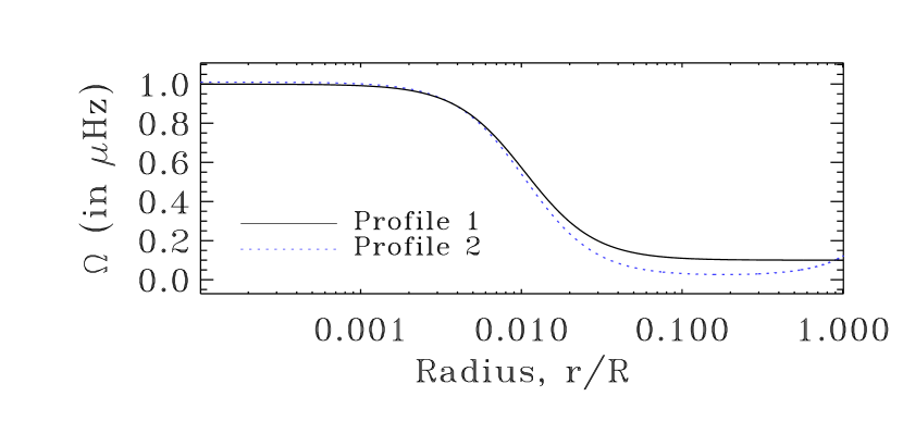
One can also investigate the use of these inequalities in red giant stars. However, these seem to be less effective for such stars, since the rotation kernels are mainly sensitive to the core or surface regions and hardly in between. Accordingly, it is not too difficult to construct pairs of rotation profiles, one of which is decreasing the other not, and which produce essentially the same rotational splittings (i.e. to within some error bar). Figure 13 shows such a pair – the corresponding rotational splittings, when calculated in Model 1 (or Model 2 – these models are introduced in the following section), are within $0.01\,\mu$Hz. Indeed, as explained in Goupil et al. (2013), the rotational splittings of red-giants are primarily sensitive to the average core and surface rotation rates. Obviously, the above inequalities will not detect a positive gradient in such a situation, since there exists at least one decreasing rotation profile which reproduces the splittings within the error bars. Including higher $\ell$ modes doesn’t seem like a viable solution, as these are harder to detect and will experience a stronger trapping, either in the p- or g-mode cavities. In order to cause one of the inequalities to break down, one needs to have a rotation profile which is increasing throughout most of the star. However, this will probably cause the splittings of the p-like modes to be comparable or larger than those of the g-like modes – already a very strong indication of an increasing rotation rate prior to any tests or inversions. In the following section, we nonetheless show how the above inequalities can be useful when studying red giants.

Figure 13: (Colour online) Rotation profiles which give the similar splittings (to within $0.01\,\mu$Hz) in Model 1 (from Sect. 3.2). Profile 1 is also used to calculate the “observed” rotational splittings (using Model 2) in Sect. 3.2.

3.2 The effects of a mismatch between an observed star and the reference model

At this point a natural question arises: if the above inequalities break down is this necessarily caused by a positive gradient in the rotation profile, or can there be other causes? In what follows, we will show a situation where a slight mismatch between an “observed” star and a reference model leads to one of the inequalities breaking down, in spite of having a rotation profile where the gradient is negative everywhere. To do so, we start off with two very close 1 M_⊙ models of red-giant stars. The second model is the same as the first, except for an ad-hoc $50\%$ decrease of the density near the surface. This is achieved by multiplying the density profile by the following function:

$$f(r)=1+\frac{A\left\{1+\tanh\left[\frac{\lambda(r-r_{d})}{R}\right]\right\}}{2},$$ (51)

where $r_{d}=0.995$, $\lambda=2\times 10^{3}$, and $A=-0.5$. Table 1 gives the characteristics of these two models. We note in passing that the mass difference between these two models corresponds to $73\%$ of Mercury’s mass. Figure 14 shows the inertia of their $\ell=0$ and $1$ modes as a function of frequency, where $I_{n,\ell}=\int_{0}^{M}\|\@vec{\xi}\|^{2}\mathrm{d}m/[M\xi^{2}(R)]$.

Table 1: Characteristics of the two models. The second column gives the characteristics of Model 1, whereas the third column gives the relative difference between Models 2 and 1.

Quantity	Model 1	Relative difference
Mass (in M⊙)	$1.000$	$-1.22\times 10^{-7}$
Radius (in R⊙)	$4.107$	$0$
$\sqrt{GM/R^{3}}$ (in $\mu$Hz)	$12.00$	$-6.1\times 10^{-8}$

Figure 14: (colour online) Inertias of $\ell=0$ and $1$ modes in models 1 and 2 as a function of frequency.

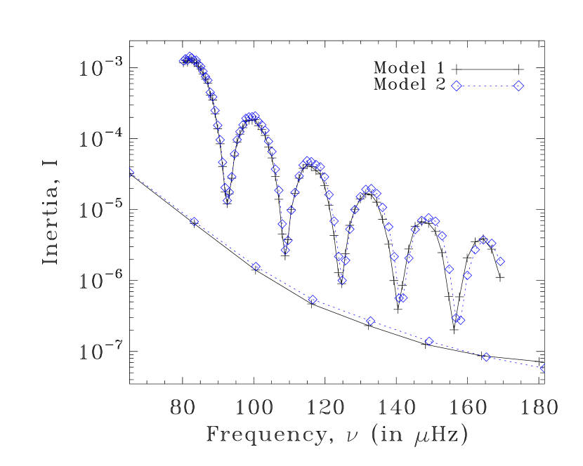
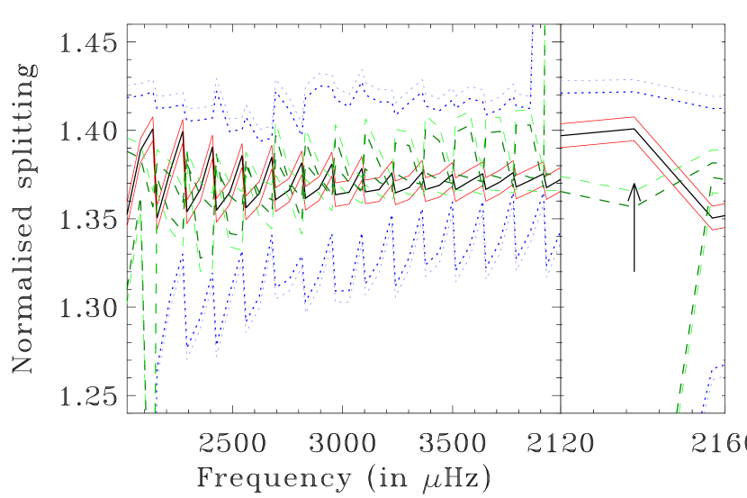
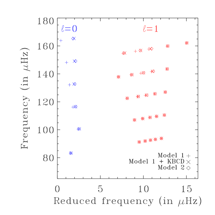
In what follows, the frequencies of Model 2 will be treated as the observations, and Model 1 will be used as a reference model. Furthermore, the “observed” frequency spectrum will include all of the $\ell=0$ modes over a given frequency range, and only a subset of the $\ell=1$ modes. Indeed, only the most p-like dipole modes are expected to be visible in observed stars. We therefore selected the dipole modes at local minima of the inertia curve as well as the adjacent 2 modes on either side. Figure 15 shows an echelle diagram with the frequencies from both models. We assume $1\sigma$ error bars of $0.01$ $\mu$Hz on the frequencies, which is typical for the Kepler mission. Table 2 gives the value of $\chi^{2}_{\mathrm{red}}=\frac{1}{M}\sum_{i=1}^{M}\left(\frac{\nu^{\mathrm{ref}}_{i}-\nu^{\mathrm{obs}}_{i}}{\sigma_{i}}\right)^{2}$ where $M$ is the number of frequencies. This quantity characterises the departure of the frequency spectrum of Model 1 from that of Model 2.

Figure 15: Echelle diagram comparing the frequencies of Model 1 (with and without the KBCD surface corrections) and Model 2.

Table 2: Seismic $\chi^{2}_{\mathrm{red}}$ values for Model 1, with and without the KBCD surface corrections.

Frequency set	$\chi^{2}_{\mathrm{red}}$
Model 1	1364.5
Model 1 + KBCD	19.4

As can be seen from Table 2, the pulsation spectrum of Model 1 is a poor fit to the observations. Our observational error bars would therefore exclude Model 1 immediately. However, surface corrections based on Kjeldsen et al. (2008) (KBCD, hereafter) are frequently included in seismic studies of observed stars. We therefore applied such corrections to the frequencies of Model 1, using the following formula:

$$\nu_{n,\ell}^{\mathrm{corrected}}=\nu_{n,\ell}+\frac{a_{\mathrm{KBCD}}\left(\frac{\nu_{n,\ell}}{\nu_{0}}\right)^{b_{\mathrm{KBCD}}}}{Q_{n,\ell}}$$ (52)

where $\nu_{n,\ell}$ are the original frequencies, $\nu_{n,\ell}^{\mathrm{corrected}}$ the corrected frequencies, $\nu_{0}$ a reference frequency, $a_{\mathrm{KBCD}}$ a multiplicative constant, $b_{\mathrm{KBCD}}$ the exponent used in KBCD’s power law, and $Q_{n,\ell}$ the mode’s inertia, divided by the inertia of an $\ell=0$ mode interpolated to the same frequency (e.g. Aerts et al., 2010, page 470). We choose the values $\nu_{0}=125\,\mu$Hz, which is in the middle of the frequency range, $a_{\mathrm{KBCD}}=0.40315$ in order to reproduce as accurately as possible the frequency deviations in Model 2, and $b_{\mathrm{KBCD}}=4.9$, the value obtained in KBCD after calibrating Model S to the sun. The division by $Q_{n,\ell}$ is a later addition to the formula, which proved to be necessary in the case of red giants, due to the large variations of the inertia of non-radial modes (e.g. Deheuvels et al., 2012). The second line of Table 2 shows the impact of including this surface correction. Although the $\chi^{2}_{\mathrm{red}}$ is still above $1$ and is worse than the best fitting models in Deheuvels et al. (2012), it is better than any of the best fits found in Deheuvels et al. (2014). Hence, such a model would probably be retained as a viable reference model with which to study the “observed” star (i.e. Model 2).

We calculate rotational splittings in Model 2, using the following rotation profile:

$$\Omega(r)=A+\frac{B}{1+C(r/R)^{2}}$$ (53)

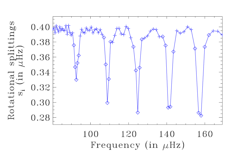
where $A=0.1$ $\mu$Hz, $B=0.9$ $\mu$Hz and $C=9\times 10^{3}$. We note that this rotation profile decreases with $r$, but still satisfies Rayleigh’s stability criterion. This rotation profile is illustrated in Fig. 13 (see Profile 1). The resultant rotational splittings for model 2 are shown in Fig. 16, and these will serve as our observations. We assume $1\sigma$ error bars of $0.007$ $\mu$Hz on these splittings, which is approximately $\sqrt{2}$ times smaller than the error bars on the frequencies, which is what you would expect from generalised $\ell=1$ splittings.

Figure 16: Rotational splittings in model 2. The diamonds correspond to the splittings which were used in this study, whereas the crosses represent those which were discarded.

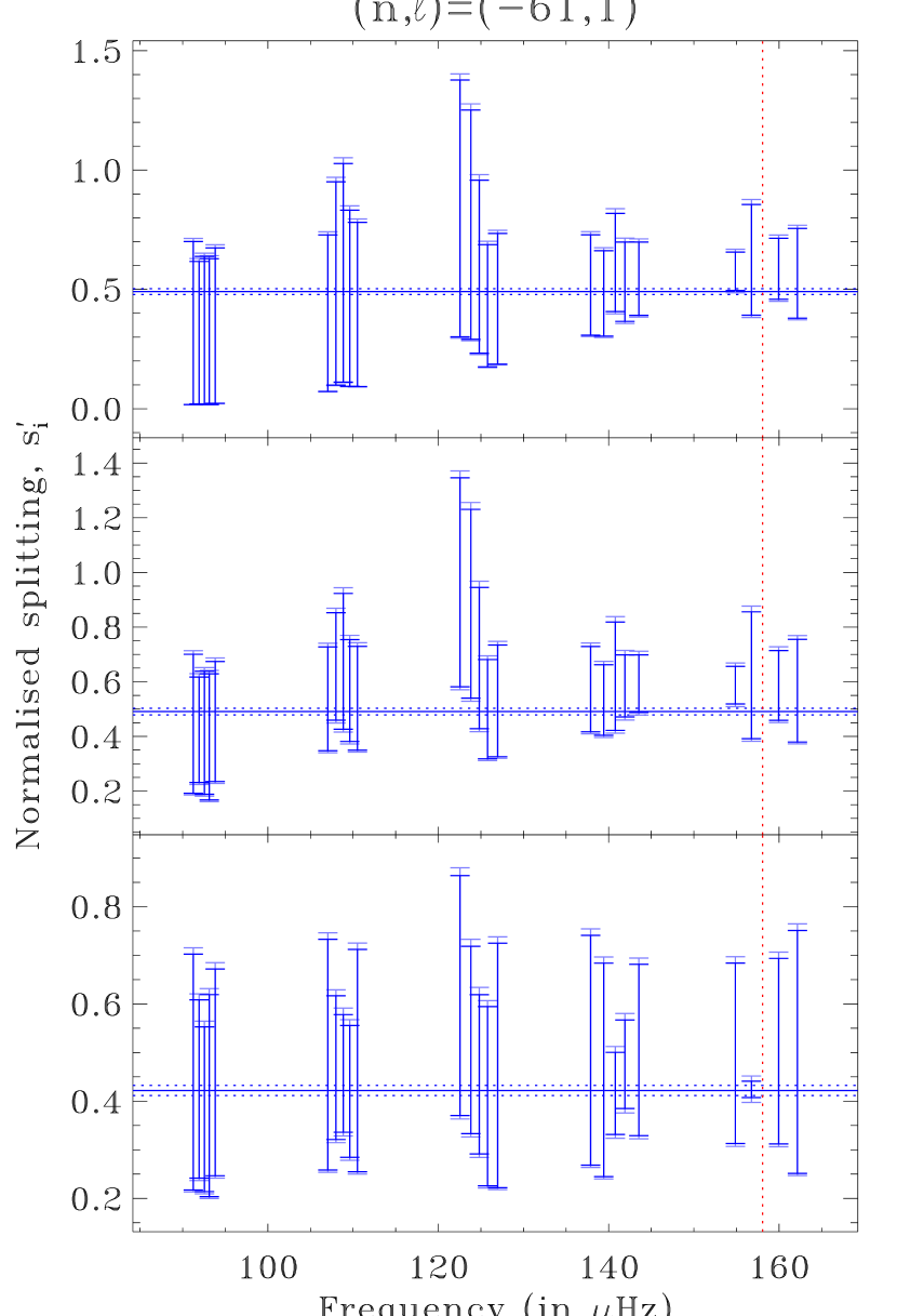
Then, we systematically apply Eq. (13) to every pair of dipole modes. For each mode, we end up with $N-1$ upper and lower bounds, where $N$ is the number of rotational splittings. Figure 17 (upper panel) shows the bounds which are obtained for one of the p-like modes in Model 1. According to this approach, this splitting is compatible with the lower and upper bounds from the other modes to within the $1.22\sigma$. However, if the centre is excluded, as explained in Sect. 2.1.2, then it is possible to find an inequality which breaks down by $5.87\sigma$. The middle panel of Figure 17 shows the bounds obtained for the same mode, but using Eq. 23 with $r_{0}=2\times 10^{-4}R$ and $R\mathcal{B}=5\times 10^{5}\,\mu$Hz. We note that the actual upper bound over the interval $[0,r_{0}]$ is $R\mathcal{B}=3.270\,\mu$Hz, i.e. more than 5 orders of magnitude smaller. A Monte-Carlo simulation based on the coefficients deduced from inequalities on mode pairs found three cases where $\varepsilon^{\prime}/\sigma^{\prime}>5.87$ in $10^{6}$ realisations, thereby indicating a false alarm probability of $3\times 10^{-6}$. The lower panel shows what happens when applying the same tests using Model 2 as a reference model. This time we set $R\mathcal{B}=3.270\,\mu$Hz to be as restrictive as possible. Even then, none of the inequalities break down, which is consistent with the fact that we are using the true model and the rotation profile is decreasing.

Figure 17: (colour online) Upper and lower bounds on a given splitting, deduced from the $N-1$ other rotational splittings, assuming that the rotation profile decreases. In the upper and middle panels, Model 1 has been used as the reference model, whereas in the lower panel, Model 2 is the reference model. In the lower two panels, a more restrictive set of inequalities is obtained by excluding the centre, as described in Sect. 2.1.2. The frequency of the original mode is shown by the red vertical dotted line, whereas the blue horizontal dotted and solid lines indicate its rotational splitting plus or minus the error bar. The dark blue solid vertical segments indicate the upper and lower bounds deduced from the other modes, and the $1\sigma$ error bars are indicated by the light blue extensions.

It is relatively straightforward to understand why Model 1 leads to a break down of one of the inequalities. Indeed, as can be seen in Fig. 14, the mode inertias of Models 1 and 2 do not match very well, especially for the high frequency p-like dipole modes. This modification of mode inertias stems from the fact that surface effects act differently on p and g-modes and will therefore shift the former with respect to the latter. This, in turn, modifies the avoided crossings which occur between them, and hence, the inertias of the resultant modes. Such an effect is likely to be strongest in red giant stars where the spacing between consecutive g-modes can be comparable to the frequency shifts caused by surface effects. In contrast, applying a surface correction recipe like the one described in KBCD merely corrects the frequencies and not the inertias. This leads to inconsistencies between the mode inertias and period spacings, as illustrated in Fig. 18, and could mask mismatches between observations and what seems to be the best-fitting model(s).

Figure 18: Normalised mode inertias as a function of averaged periods spacings (defined as $\pi_{n}=(1/\nu_{n-1}-1/\nu_{n+1})/2$, where $n$ is the radial order). The lower panel corresponds to Model 1 with a $90\,\%$ decrease in density near the surface, whereas the upper panel uses Model 1 with KBCD surface corrections, adjusted so as to match (as best as possible) the frequencies of the modified model. The increased scatter at low inertias in the upper panel illustrates the mismatch between period spacings and mode inertias.

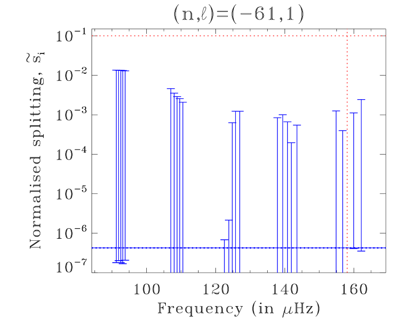
One can also apply the tests based on Rayleigh’s criterion. We therefore systematically applied Eq. (41) using the exact surface rotation rate, to every pair of modes. However, this set of inequalities turns out to be far less stringent than the first set of inequalities. Accordingly, none of them break down, even when the centre is excluded, as described in Sect. 2.2.2, using the most restrictive value of $\tilde{\mathcal{B}}$ possible. Figure 19 shows lower and upper bounds for the rotational splitting of the dipole mode $(n,\ell)=(-61,1)$ with $r_{0}/R=2\times 10^{-4}$ and $\tilde{\mathcal{B}}/R=4.037\times 10^{-4}\,\mu$Hz.

Figure 19: (colour online) Same as Fig. 17 but using the inequalities based on Rayleigh’s criterion. The centre has also been excluded, as described in the text, thereby leading to more stringent conditions. The horizontal red dotted line near the top of the figure is an upper limit deduced from the surface rotation rate. The error bars which extend off the bottom of the plot go to negative values.

One could then turn the inequalities based on Rayleigh’s criterion the other way around and search for a lower bound on the surface rotation rate. Equation (36) already provides a first condition. Applying this condition using Model 1 as the reference model leads to $\Omega(R)>6.54\times 10^{-7}\,\mu$Hz whereas Model 2 (the true model) leads to $\Omega(R)>6.04\times 10^{-7}\,\mu$Hz. The true surface rotation rate is more than 5 orders of magnitude larger, with $\Omega(R)=0.10010\,\mu$Hz. However one can also rearrange Eq. (48) to obtain a more restrictive condition:

$$\frac{\tilde{b}^{\star}\tilde{s}_{j}-\tilde{s}_{i}-\tilde{\mathcal{B}}\!\!\int_{0}^{r_{0}}\!\!\max\left[0,J_{i}(r)-\tilde{b}^{\star}J_{j}(r)\right]\mathrm{d}r}{R^{2}(\tilde{b}^{\star}-1)} \leq \Omega(R)$$ (54)

$$\frac{\tilde{s}_{i}-\tilde{a}^{\star}\tilde{s}_{j}-\tilde{\mathcal{B}}\!\!\int_{0}^{r_{0}}\!\!\max\left[0,\tilde{a}^{\star}J_{j}(r)-J_{i}(r)\right]\mathrm{d}r}{R^{2}(1-\tilde{a}^{\star})} \leq \Omega(R)$$ (55)

Applying these conditions using $r_{0}=2\times 10^{-4}$ and $\tilde{\mathcal{B}}/R=4.037\times 10^{-4}\,\mu$Hz yields $\Omega(R)\geq 4.89\times 10^{-4}\,\mu$Hz for Model 1 and $\Omega(R)\geq 1.52\times 10^{-5}\,\mu$Hz for Model 2, which is still 3 to 4 orders of magnitude below the true value, and furthermore, very model dependant. Hence, even this way around, the inequalities based on Rayleigh’s criterion only provide very weak constraints and one would probably be better off either trying to measure the rotation rate through photometric modulation induced by spots (if present) or through spectroscopy. Alternatively, one could apply the relation derived by Goupil et al. (2013) which relates the ratio between the average surface and core rotation rates of red giants to the slope of the rotational splittings as a function of $\zeta$, the ratio of the kinetic energy of the mode in the g-mode cavity to the total kinetic energy. Such a relation has already been tested on $6$ subgiants observed by Kepler and shown to agree, in most cases, with results based on inversions (Deheuvels et al., 2014).

4 Discussion

In this article, we have derived various inequalities which can be used to check whether a rotation profile has a negative gradient or satisfies Rayleigh’s stability criterion, for a given reference model. We explored how these inequalities may be used in practical situations by investigating various test cases. In the first test case, a rotation profile which satisfies neither the assumption $\frac{\mathrm{d}\Omega}{\mathrm{d}r}\leq 0$ everywhere nor Rayleigh’s criterion was imposed on Model S (Christensen-Dalsgaard et al., 1996). A set of $44$ splittings for modes with $\ell=1$ to $3$ were used in the various tests. The above inequalities were able to detect the presence of a positive gradient, but were unable to show a violation of Rayleigh’s criterion. Although an inversion also suggested the presence of a positive gradient, the resultant conclusions remained less firm than those derived by the inequalities. A second test case, also based upon Model S, used a different profile which also contained a region positive gradient on the rotation profile and one where the angular momentum is decreasing. This second case used a set of $282$ modes (with $\ell=1$ to $20$), thereby enabling a clear detection of both of these regions using inversions. In contrast, the above inequalities failed to detect the positive gradient in the rotation profile, probably as a result of the narrowness of this region. However, these were able to detect a violation of Rayleigh’s criterion, even in situations where inversions yielded poor results, provided modes with $\ell\geq 8$ were included. We expect that this lower limit on the $\ell$ value is dependant on both the way in which the rotation profile violates Rayleigh’s criterion and on the size of the error bars on the rotational splittings.

We also looked at other ways in which the inequalities may break down. For this purpose, we considered two models of red-giants which were identical except for an ad-hoc near-surface modification of the density profile in the second model. The first model was then used as a reference model in trying to interpret the rotational splittings of the second model, which were based on a rotation profile which has a negative gradient everywhere and which obeys Rayleigh’s criterion. It turned out that one of the inequalities based on the rotation profile’s gradient was violated, whereas all of the inequalities based on Rayleigh’s criterion were satisfied. The reason for this is that the mode inertias differ in the two models, especially at high frequencies. This may come as a surprise since only the outer $0.5\,\%$ or so is different between the two models. However, as argued above, near-surface effects shifts the frequencies of p-like modes relative to those of the g-like modes, thereby modifying the avoided crossings which occur between the two, and hence the resultant inertias. Frequency correction recipes for near-surface effects, such as the one presented in Kjeldsen et al. (2008), are able to mask the frequency differences between the two models, but they do not correct the mode inertias, thereby leading to erroneous conclusions on the rotation profile as shown in this test case.

This leads to the natural question as to what to do if one or several inequalities are violated by a set of observed rotational splittings. In answer to this question, one needs to consider the following options. First, a different, more suitable, reference model needs to be found. We expect that in the case of red giants, the above inequalities could be quite constraining, due to very different mode trappings, and may therefore provide an indirect way of testing the structure of the reference model. Furthermore, such stars are the most likely candidates to having a rotation profile which decreases outward due to the spin-up of the core as it contracts and the slowing down of the envelope as it expands. Of course, a direct comparison of the non-radial mode frequencies will very likely provide tighter constraints, but so far, no one has yet fitted a red-giant model to within $1\sigma$ of a set observed frequencies. Hence, if one adopts less stringent constraints on the selection of the model, and/or if frequency surface-corrections are included, the above criteria will be useful in determining beforehand whether or not the chosen reference model is compatible with a decreasing rotation profile. The second option, is to consider that the rotation profile doesn’t have a negative gradient throughout the star and/or violates Rayleigh’s stability criterion (depending on which inequalities are not satisfied). As was already stated in the introduction, there is convincing evidence of stars where the gradient of the rotation profile is positive, at least in localised regions (Schou et al., 1998; Kurtz et al., 2014). This raises the open questions as to how often such a situation occurs, and whether even a red giant couldn’t have a localised region with a positive rotation gradient, for example, in the outer convective envelope. However, one must not forget that the above criteria are not necessarily the most effective at detecting a rotation profile with a positive gradient. Accordingly, a mismatch between the reference model and the observed star may be a more likely explanation, which brings us back to the first option. A last option would be to consider that the rotation profile is too rapid to be described by first order effects, thereby violating the assumptions in this work. In such a situation, it would no longer be possible to apply linear inversion theory, except perhaps on generalised rotational splittings (defined as the frequency difference between prograde modes and their retrograde counterparts) of acoustic modes in stars with nearly uniform rotation profiles (Reese et al., 2009). Recent works (Reese et al., 2006; Ballot et al., 2010; Ouazzani et al., 2013) have, however, shown up to what point a first order description of the effects of rotation are valid, and can therefore be used to decide whether or not the criteria described in this paper are applicable.

Appendix A Attempting to construct a decreasing rotation profile when Eq. (23) is satisfied

We start by introducing the following radial coordinates:

$$r_{a^{\star}}=\operatorname*{arg\,min}_{r\in[r_{0},R]}\left(\frac{I_{i}(r)}{I_{j}(r)}\right),\qquad r_{b^{\star}}=\operatorname*{arg\,max}_{r\in[r_{0},R]}\left(\frac{I_{i}(r)}{I_{j}(r)}\right).$$ (56)

and define a profile as follows (where we have assumed $r_{a^{\star}}<r_{b^{\star}}$):

$$\Omega(r)=\left\{\begin{array}[]{ll}\lambda+\mu&\mbox{ if }r_{0}\leq r\leq r_{a^{\star}}\\ \mu&\mbox{ if }r_{a^{\star}}<r\leq r_{b^{\star}}\\ 0&\mbox{ if }r_{b^{\star}}<r\leq R\end{array}\right..$$ (57)

A similar solution can be obtained if $r_{b^{\star}}<r_{a^{\star}}$. In this definition, we have deliberately postponed defining the rotation profile over the interval $[0,r_{0}[$, except that we will impose its continuity at $r_{0}$ (except if $r_{0}=r_{a^{\star}}$). Inserting this expression into Eq. (19) then yields the following system:

$$s^{\prime}_{i}+\int_{0}^{r_{0}}\frac{\mathrm{d}\Omega}{\mathrm{d}r}I_{i}(r)\mathrm{d}r = \lambda I_{i}(r_{a^{\star}})+\mu I_{i}(r_{b^{\star}}),$$ (58)

$$s^{\prime}_{j}+\int_{0}^{r_{0}}\frac{\mathrm{d}\Omega}{\mathrm{d}r}I_{j}(r)\mathrm{d}r = \lambda I_{j}(r_{a^{\star}})+\mu I_{j}(r_{b^{\star}}),$$ (59)

the solution of which is:

$$\lambda = \frac{1}{I_{j}(r_{a^{\star}})}\left\{\frac{b^{\star}s^{\prime}_{j}-s^{\prime}_{i}+\int_{0}^{r_{0}}\frac{\mathrm{d}\Omega}{\mathrm{d}r}\left[b^{\star}I_{j}(r)-I_{i}(r)\right]\mathrm{d}r}{b^{\star}-a^{\star}}\right\},$$ (60)

$$\mu = \frac{1}{I_{j}(r_{b^{\star}})}\left\{\frac{s^{\prime}_{i}-a^{\star}s^{\prime}_{j}+\int_{0}^{r_{0}}\frac{\mathrm{d}\Omega}{\mathrm{d}r}\left[I_{i}(r)-a^{\star}I_{j}(r)\right]\mathrm{d}r}{b^{\star}-a^{\star}}\right\}.$$ (61)

From this we deduce that Eq. (20) is a sufficient condition to ensure that $\lambda$ and $\mu$ are positive, and hence that $\Omega$ is decreasing. In contrast, Eq. (23), does not ensure that $\lambda$ and $\mu$ are positive. To see this, we re-express the numerator of Eq. (60) as follows:

$$\underbrace{b^{\star}s^{\prime}_{j}-s^{\prime}_{i}-\int_{0}^{r_{0}}\frac{\mathrm{d}\Omega}{\mathrm{d}r}\max\left[0,I_{i}(r)-b^{\star}I_{j}(r)\right]\mathrm{d}r}_{I}$$

$$\underbrace{-\int_{0}^{r_{0}}\frac{\mathrm{d}\Omega}{\mathrm{d}r}\min\left[0,I_{i}(r)-b^{\star}I_{j}(r)\right]\mathrm{d}r}_{II}.$$

In order to ensure that the term $I$ is positive according to Eq. (23), one needs to set $\frac{\mathrm{d}\Omega}{\mathrm{d}r}$ to $-\mathcal{B}$ over the interval where $I_{i}(r)-b^{\star}I_{j}(r)$ is positive. Term $II$ is necessarily smaller or equal to zero. In order to cancel it out, $\frac{\mathrm{d}\Omega}{\mathrm{d}r}$ needs to be zero over the interval where $I_{i}(r)-b^{\star}I_{j}(r)$ is negative. Likewise, in order to ensure that $\mu$ is positive, one would need to make sure $\frac{\mathrm{d}\Omega}{\mathrm{d}r}=-\mathcal{B}$ when $a^{\star}I_{i}(r)-I_{j}(r)$ is positive, and $\frac{\mathrm{d}\Omega}{\mathrm{d}r}=0$ otherwise. However, there is no guarantee that these two sets of conditions are compatible.