Schwarz waveform relaxation method for one dimensional Schrödinger equation with general potential

C. Besse christophe.besse@math.univ-toulouse.fr F. Xing feng.xing@unice.fr Institut de Mathématiques de Toulouse UMR5219, Université de Toulouse; CNRS, UPS IMT, F-31062 Toulouse Cedex 9, France. Maison de la Simulation, CEA Saclay France & Laboratoire Paul Painlevé, Université Lille Nord de France.
Abstract

In this paper, we apply the Schwarz Waveform Relaxation (SWR) method to the one dimensional Schrödinger equation with a general linear or a nonlinear potential. We propose a new algorithm for the Schrödinger equation with time independent linear potential, which is robust and scalable up to 500 subdomains. It reduces significantly computation time compared with the classical algorithms. Concerning the case of time dependent linear potential or the nonlinear potential, we use a preprocessed linear operator for the zero potential case as preconditioner which lead to a preconditioned algorithm. This ensures high scalability. Besides, some newly constructed absorbing boundary conditions are used as the transmission condition and compared numerically.

keywords:
Schrödinger equation, Schwarz Waveform Relaxation method, Absorbing boundary conditions, Parallel algorithms.
journal: Journal of Computational Physics

1 Introduction

Schwarz waveform relaxation method (SWR) is one class of the domain decomposition methods for time dependent partial differential equations. The time-space domain is decomposed into subdomains. The solution is computed on each subdomain for whole time interval and exchange the time-space boundary value. Some articles are devoted to this method for linear Schrödinger equation [1, 2], advection reaction diffusion equations [3, 4, 5], wave equations [6, 7] and Maxwell’s equation [8].

This paper deals with the SWR method without overlap for the one dimensional Schrödinger equation defined on a bounded spatial domain (a0,b0)subscript𝑎0subscript𝑏0(a_{0},b_{0}), a0,b0subscript𝑎0subscript𝑏0a_{0},b_{0}\in\mathbb{R} and t(0,T)𝑡0𝑇t\in(0,T). The Schrödinger equation with homogeneous Neumann boundary condition reads

{u:=(it+xx+𝒱)u=0,(t,x)(0,T)×(a0,b0),u(0,x)=u0(x),x(a0,b0),𝐧u(t,x)=0,x=a0,b0,casesformulae-sequenceassign𝑢𝑖subscript𝑡subscript𝑥𝑥𝒱𝑢0𝑡𝑥0𝑇subscript𝑎0subscript𝑏0missing-subexpressionformulae-sequence𝑢0𝑥subscript𝑢0𝑥𝑥subscript𝑎0subscript𝑏0missing-subexpressionformulae-sequencesubscript𝐧𝑢𝑡𝑥0𝑥subscript𝑎0subscript𝑏0missing-subexpression\left\{\begin{array}[]{ll}\mathscr{L}u:=(i\partial_{t}+\partial_{xx}+\mathscr{V})u=0,\ (t,x)\in(0,T)\times(a_{0},b_{0}),\\ u(0,x)=u_{0}(x),\ x\in(a_{0},b_{0}),\\ \partial_{\mathbf{n}}u(t,x)=0,\ x=a_{0},b_{0},\end{array}\right. (1)

where \mathscr{L} is the Schrödinger operator, 𝐧subscript𝐧\partial_{\mathbf{n}} is the normal directive, the initial value u0L2()subscript𝑢0superscript𝐿2u_{0}\in L^{2}(\mathbb{R}) and 𝒱𝒱\mathscr{V} is a real potential. We consider both linear and nonlinear potentials:

  1. 1.

    𝒱=V(t,x)𝒱𝑉𝑡𝑥\mathscr{V}=V(t,x),

  2. 2.

    𝒱=f(u)𝒱𝑓𝑢\mathscr{V}=f(u), ex. 𝒱=|u|2𝒱superscript𝑢2\mathscr{V}=|u|^{2}.

In order to perform domain decomposition method, the time-space domain (0,T)×(a0,b0)0𝑇subscript𝑎0subscript𝑏0(0,T)\times(a_{0},b_{0}) is decomposed into N𝑁N subdomains Θj=(0,T)×ΩjsubscriptΘ𝑗0𝑇subscriptΩ𝑗\Uptheta_{j}=(0,T)\times\Omega_{j}, Ωj=(aj,bj)subscriptΩ𝑗subscript𝑎𝑗subscript𝑏𝑗\Omega_{j}=(a_{j},b_{j}) without overlap as shown in Figure 1 for N=3𝑁3N=3.

x𝑥xt𝑡ta0=a1subscript𝑎0subscript𝑎1a_{0}=a_{1}b1=a2subscript𝑏1subscript𝑎2b_{1}=a_{2}b2=a3subscript𝑏2subscript𝑎3b_{2}=a_{3}b2=b0subscript𝑏2subscript𝑏0b_{2}=b_{0}T𝑇T(0,T)×Ω10𝑇subscriptΩ1(0,T)\times\Omega_{1}(0,T)×Ω20𝑇subscriptΩ2(0,T)\times\Omega_{2}(0,T)×Ω30𝑇subscriptΩ3(0,T)\times\Omega_{3}𝐧2subscript𝐧2\mathbf{n}_{2}𝐧2subscript𝐧2\mathbf{n}_{2}
Figure 1: Domain decomposition without overlap, N=3𝑁3N=3.

The classical SWR algorithm consists in applying the sequence of iterations for j=2,3,,N1𝑗23𝑁1j=2,3,...,N-1

{ujk+1=0,(t,x)Θj,ujk+1(0,x)=u0(x),xΩj,Bjujk+1=Bjuj1k,x=aj,Bjujk+1=Bjuj+1k,x=bj.casessuperscriptsubscript𝑢𝑗𝑘10𝑡𝑥subscriptΘ𝑗subscriptsuperscript𝑢𝑘1𝑗0𝑥subscript𝑢0𝑥𝑥subscriptΩ𝑗subscript𝐵𝑗superscriptsubscript𝑢𝑗𝑘1subscript𝐵𝑗superscriptsubscript𝑢𝑗1𝑘𝑥subscript𝑎𝑗subscript𝐵𝑗superscriptsubscript𝑢𝑗𝑘1subscript𝐵𝑗superscriptsubscript𝑢𝑗1𝑘𝑥subscript𝑏𝑗\left\{\begin{array}[]{ll}\mathscr{L}u_{j}^{k+1}=0,&(t,x)\in\Uptheta_{j},\\[2.84526pt] u^{k+1}_{j}(0,x)=u_{0}(x),&x\in\Omega_{j},\\[2.84526pt] B_{j}u_{j}^{k+1}=B_{j}u_{j-1}^{k},&x=a_{j},\\[2.84526pt] B_{j}u_{j}^{k+1}=B_{j}u_{j+1}^{k},&x=b_{j}.\end{array}\right. (2)

The two extremal subdomains require special treatment since the Neumann boundary condition is imposed in (1) at the points a0subscript𝑎0a_{0} and b0subscript𝑏0b_{0}.

{u1k+1=0,(t,x)Θ1,u1k+1(0,x)=u0(x),xΩ1,𝐧1u1k+1=0,x=a1,B1u1k+1=B1u2k,x=b1,casesformulae-sequencesuperscriptsubscript𝑢1𝑘10𝑡𝑥subscriptΘ1missing-subexpressionformulae-sequencesubscriptsuperscript𝑢𝑘110𝑥subscript𝑢0𝑥𝑥subscriptΩ1missing-subexpressionformulae-sequencesubscriptsubscript𝐧1superscriptsubscript𝑢1𝑘10𝑥subscript𝑎1missing-subexpressionformulae-sequencesubscript𝐵1superscriptsubscript𝑢1𝑘1subscript𝐵1superscriptsubscript𝑢2𝑘𝑥subscript𝑏1missing-subexpression\displaystyle\left\{\begin{array}[]{ll}\mathscr{L}u_{1}^{k+1}=0,(t,x)\in\Uptheta_{1},\\[2.84526pt] u^{k+1}_{1}(0,x)=u_{0}(x),x\in\Omega_{1},\\[2.84526pt] \partial_{\mathbf{n}_{1}}u_{1}^{k+1}=0,x=a_{1},\\[2.84526pt] B_{1}u_{1}^{k+1}=B_{1}u_{2}^{k},x=b_{1},\end{array}\right. {uNk+1=0,(t,x)ΘN,uNk+1(0,x)=u0(x),xΩN,BNuNk+1=BNuN1k,x=aN,𝐧NuNk+1=0,x=bN.casesformulae-sequencesuperscriptsubscript𝑢𝑁𝑘10𝑡𝑥subscriptΘ𝑁missing-subexpressionformulae-sequencesubscriptsuperscript𝑢𝑘1𝑁0𝑥subscript𝑢0𝑥𝑥subscriptΩ𝑁missing-subexpressionformulae-sequencesubscript𝐵𝑁superscriptsubscript𝑢𝑁𝑘1subscript𝐵𝑁superscriptsubscript𝑢𝑁1𝑘𝑥subscript𝑎𝑁missing-subexpressionformulae-sequencesubscriptsubscript𝐧𝑁superscriptsubscript𝑢𝑁𝑘10𝑥subscript𝑏𝑁missing-subexpression\displaystyle\left\{\begin{array}[]{ll}\mathscr{L}u_{N}^{k+1}=0,(t,x)\in\Uptheta_{N},\\[2.84526pt] u^{k+1}_{N}(0,x)=u_{0}(x),x\in\Omega_{N},\\[2.84526pt] B_{N}u_{N}^{k+1}=B_{N}u_{N-1}^{k},x=a_{N},\\[2.84526pt] \partial_{\mathbf{n}_{N}}u_{N}^{k+1}=0,x=b_{N}.\end{array}\right.

The notation ujksuperscriptsubscript𝑢𝑗𝑘u_{j}^{k} denotes the solution on subdomain Θj=(0,T)×(aj,bj)subscriptΘ𝑗0𝑇subscript𝑎𝑗subscript𝑏𝑗\Uptheta_{j}=(0,T)\times(a_{j},b_{j}) at iteration k=0,1,2,𝑘012k=0,1,2,... of the SWR algorithm. The boundary information is transmitted with adjacent subdomains Θj1subscriptΘ𝑗1\Uptheta_{j-1} and Θj+1subscriptΘ𝑗1\Uptheta_{j+1} through the transmission operators Bjsubscript𝐵𝑗B_{j}.

The transmission condition is one of the key issues for this method. For the linear Schrödinger equation, the SWR method with or without overlap is introduced and analyzed by Halpern and Szeftel in [1]. For the decomposition without overlap, if 𝒱𝒱\mathscr{V} is a constant, they use an optimal transmission condition given by the underlying transparent boundary condition. However, the transparent boundary condition is not always available for a variable potential. Robin transmission condition and quasi-optimal transmission condition are therefore used and are named as optimized Schwarz waveform relaxation algorithm and quasi-optimal Schwarz waveform relaxation algorithm respectively. In both cases, the transmission operator is written as

Bj=𝐧j+Sj,subscript𝐵𝑗subscriptsubscript𝐧𝑗subscript𝑆𝑗B_{j}=\partial_{\mathbf{n}_{j}}+S_{j}, (3)

where the operator Sjsubscript𝑆𝑗S_{j} is

Robin:Sj=ip,p+,Quasi-optimal:Sj=itV|aj,bj,:Robinformulae-sequencesubscript𝑆𝑗𝑖𝑝𝑝superscriptQuasi-optimal:subscript𝑆𝑗𝑖subscript𝑡evaluated-at𝑉subscript𝑎𝑗subscript𝑏𝑗\text{Robin}:\ S_{j}=-ip,\ p\in\mathbb{R}^{+},\quad\text{Quasi-optimal}:\ S_{j}=\sqrt{-i\partial_{t}-V|_{a_{j},b_{j}}},

and 𝐧jsubscript𝐧𝑗\mathbf{n}_{j} denotes the outwardly unit normal vector at ajsubscript𝑎𝑗a_{j} or bjsubscript𝑏𝑗b_{j}. Recently, Antoine, Lorin and Bandrauk [9] consider the general Schrödinger equation. On the interface between subdomains, they propose to use recent absorbing conditions as transmission condition, which is also an idea that we follow in this paper.

In recent years, some absorbing operators for one dimensional Schrödinger equation have been constructed by using some adaptations of pseudo-differential techniques [10, 11, 12, 13]. We use them here as the transmission operators in (3) and expect to get good convergence properties.

We are also interested in this article about the effectivness of the method on parallel computers. Another import issue for the method is therefore the scalability. As we know, without additional considerations, the more subdomains are used to decomposed (a0,b0)subscript𝑎0subscript𝑏0(a_{0},b_{0}), the more iterations are required for SWR algorithm to reach convergence. Thus, the total computation time could hardly decrease significantly. In this paper, we propose two solutions: a new scalable algorithm if the potential is independent of time and a preconditioned algorithm for general potentials.

This paper is organized as follows. In section 2, we present the transmission conditions which are used in this paper for the classical SWR algorithm, and the discretization that plays an important role for the analyses of the interface problem in Section 3. In Section 4 and 5, we present the new algorithm for time independent linear potential and the preconditioned algorithm for general potentials. Some numerical results are shown in Section 6. Finally, we draw a conclusion in the last section.

2 SWR algorithm and discretization

2.1 Transmission conditions

The transmission conditions on boundary points ajsubscript𝑎𝑗a_{j} and bjsubscript𝑏𝑗b_{j} are given thanks to the relation

Bj=𝐧j+Sj,subscript𝐵𝑗subscriptsubscript𝐧𝑗subscript𝑆𝑗B_{j}=\partial_{\mathbf{n}_{j}}+S_{j}, (4)

where the operators Sjsubscript𝑆𝑗S_{j} could take different forms. Besides the Robin transmission condition, we propose in this paper to use the operators Sjsubscript𝑆𝑗S_{j} coming from the artificial boundary conditions for (1) defined in [13, 11, 12, 14] for a linear or nonlinear potential 𝒱(t,x,u)𝒱𝑡𝑥𝑢\mathscr{V}(t,x,u). The authors propose three families of conditions written as

𝐧u+SlMu=0,subscript𝐧𝑢superscriptsubscript𝑆𝑙𝑀𝑢0\partial_{\mathbf{n}}u+S_{l}^{M}u=0,

on the boundary of considered computation domain, M𝑀M denotes the order of the artificial boundary conditions. We index by l𝑙l these families of boundary conditions: l=0𝑙0l=0 for potential strategy, l=1𝑙1l=1 for gauge change strategy and l=2𝑙2l=2 for Padé approximation strategy. We recall here the definition of operators SlMsuperscriptsubscript𝑆𝑙𝑀S_{l}^{M} for the different strategies.

Potential strategy l=0𝑙0l=0 ([13])

Order 2::Order2absent\displaystyle\mathrm{Order}\ 2: S02=eiπ4t1/2,superscriptsubscript𝑆02superscript𝑒𝑖𝜋4superscriptsubscript𝑡12\displaystyle\quad S_{0}^{2}=e^{-i\frac{\pi}{4}}\partial_{t}^{1/2},
Order 3::Order3absent\displaystyle\mathrm{Order}\ 3: S03=S02eiπ4𝒱2It1/2,superscriptsubscript𝑆03superscriptsubscript𝑆02superscript𝑒𝑖𝜋4𝒱2superscriptsubscript𝐼𝑡12\displaystyle\quad S_{0}^{3}=S_{0}^{2}-e^{i\frac{\pi}{4}}\frac{\mathscr{V}}{2}I_{t}^{1/2},
Order 4::Order4absent\displaystyle\mathrm{Order}\ 4: S04=S03i𝐧𝒱4It,superscriptsubscript𝑆04superscriptsubscript𝑆03𝑖subscript𝐧𝒱4subscript𝐼𝑡\displaystyle\quad S_{0}^{4}=S_{0}^{3}-i\frac{\partial_{\mathbf{n}}\mathscr{V}}{4}I_{t},

where the fractional half-order derivative operator t1/2superscriptsubscript𝑡12\partial_{t}^{1/2} applied to a function hh is defined by

t1/2h(t)=1πt0th(s)ts𝑑s,superscriptsubscript𝑡12𝑡1𝜋subscript𝑡superscriptsubscript0𝑡𝑠𝑡𝑠differential-d𝑠\partial_{t}^{1/2}h(t)=\frac{1}{\sqrt{\pi}}\partial_{t}\int_{0}^{t}\frac{h(s)}{\sqrt{t-s}}ds,

the half-order integration operator It1/2superscriptsubscript𝐼𝑡12I_{t}^{1/2} and the integration operator are given by

It1/2h(t)=1π0th(s)ts𝑑s,Ith(t)=0th(s)𝑑s.formulae-sequencesuperscriptsubscript𝐼𝑡12𝑡1𝜋superscriptsubscript0𝑡𝑠𝑡𝑠differential-d𝑠subscript𝐼𝑡𝑡superscriptsubscript0𝑡𝑠differential-d𝑠I_{t}^{1/2}h(t)=\frac{1}{\sqrt{\pi}}\int_{0}^{t}\frac{h(s)}{\sqrt{t-s}}ds,\ \ I_{t}h(t)=\int_{0}^{t}h(s)ds.

Gauge change strategy l=1𝑙1l=1 ([11, 12])

Order 2::Order2absent\displaystyle\mathrm{Order}\ 2: S12=eiπ4ei𝒱(t,x)t1/2(ei𝒱(t,x)),\displaystyle\quad S_{1}^{2}=e^{-i\frac{\pi}{4}}e^{i\mathcal{V}(t,x)}\partial_{t}^{1/2}(e^{-i\mathcal{V}(t,x)}\cdot),
Order 4::Order4absent\displaystyle\mathrm{Order}\ 4: S14=S12isgn(𝐧𝒱)|𝐧𝒱|2ei𝒱(t,x)It(|𝐧𝒱|2ei𝒱(t,x)),\displaystyle\quad S_{1}^{4}=S_{1}^{2}-i\mathrm{sgn}(\partial_{\mathbf{n}}\mathscr{V})\frac{\sqrt{|\partial_{\mathbf{n}}\mathscr{V}|}}{2}e^{i\mathcal{V}(t,x)}I_{t}(\frac{\sqrt{|\partial_{\mathbf{n}}\mathscr{V}|}}{2}e^{-i\mathcal{V}(t,x)}\cdot),

where sgn()𝑠𝑔𝑛sgn(\cdot) is the sign function and

𝒱(t,x)=0t𝒱(s,x,u(s,x))𝑑s.𝒱𝑡𝑥superscriptsubscript0𝑡𝒱𝑠𝑥𝑢𝑠𝑥differential-d𝑠\mathcal{V}(t,x)=\int_{0}^{t}\mathscr{V}(s,x,u(s,x))ds.

Padé approximation strategy l=2𝑙2l=2 ([11, 12])

Order 2::Order2absent\displaystyle\mathrm{Order}\ 2: S22=iit+𝒱,superscriptsubscript𝑆22𝑖𝑖subscript𝑡𝒱\displaystyle\quad S_{2}^{2}=-i\sqrt{i\partial_{t}+\mathscr{V}},
Order 4::Order4absent\displaystyle\mathrm{Order}\ 4: S24=S22+sgn(𝐧𝒱)|𝐧𝒱|2(it+𝒱)1(|𝐧𝒱|2).\displaystyle\quad S_{2}^{4}=S_{2}^{2}+\mathrm{sgn}(\partial_{\mathbf{n}}\mathscr{V})\frac{\sqrt{|\partial_{\mathbf{n}}\mathscr{V}|}}{2}\big{(}i\partial_{t}+\mathscr{V}\big{)}^{-1}\Big{(}\frac{\sqrt{|\partial_{\mathbf{n}}\mathscr{V}|}}{2}\cdot\Big{)}.

2.2 Discretization

The aim of this subsection is to present the discretization of the Schrödinger equation with a linear potential 𝒱=V(t,x)𝒱𝑉𝑡𝑥\mathscr{V}=V(t,x) or a nonlinear potential 𝒱=f(u)𝒱𝑓𝑢\mathscr{V}=f(u).

2.2.1 Case of linear potential

First, we describe the discretization of the linear Schrödinger equation. We discretize the time interval (0,T)0𝑇(0,T) uniformly with NTsubscript𝑁𝑇N_{T} intervals and define Δt=T/NTΔ𝑡𝑇subscript𝑁𝑇\Delta t=T/N_{T} to be the time step. A semi-discrete approximation adapted to the Schrödinger equation on (0,T)×(aj,bj),j=1,2,,Nformulae-sequence0𝑇subscript𝑎𝑗subscript𝑏𝑗𝑗12𝑁(0,T)\times(a_{j},b_{j}),j=1,2,...,N is given by the semi-discrete Crank-Nicolson scheme

iuj,nkuj,n1kΔt+xxuj,nk+uj,n1k2+Vn+Vn12uj,nk+uj,n1k2=0, 1nNT,formulae-sequence𝑖superscriptsubscript𝑢𝑗𝑛𝑘superscriptsubscript𝑢𝑗𝑛1𝑘Δ𝑡subscript𝑥𝑥superscriptsubscript𝑢𝑗𝑛𝑘superscriptsubscript𝑢𝑗𝑛1𝑘2subscript𝑉𝑛subscript𝑉𝑛12superscriptsubscript𝑢𝑗𝑛𝑘superscriptsubscript𝑢𝑗𝑛1𝑘201𝑛subscript𝑁𝑇i\frac{u_{j,n}^{k}-u_{j,n-1}^{k}}{\Delta t}+\partial_{xx}\frac{u_{j,n}^{k}+u_{j,n-1}^{k}}{2}+\frac{V_{n}+V_{n-1}}{2}\frac{u_{j,n}^{k}+u_{j,n-1}^{k}}{2}=0,\ 1\leqslant n\leqslant N_{T},

and uj,0k=u(0,x)superscriptsubscript𝑢𝑗0𝑘𝑢0𝑥u_{j,0}^{k}=u(0,x) for x(aj,bj)𝑥subscript𝑎𝑗subscript𝑏𝑗x\in(a_{j},b_{j}). The unknown function uj,nk(x)superscriptsubscript𝑢𝑗𝑛𝑘𝑥u_{j,n}^{k}(x) is an approximation of the solution ujk(nΔt,x)superscriptsubscript𝑢𝑗𝑘𝑛Δ𝑡𝑥u_{j}^{k}(n\Delta t,x) to the Schrödinger equation at time tn=nΔtsubscript𝑡𝑛𝑛Δ𝑡t_{n}=n\Delta t on subdomain ΩjsubscriptΩ𝑗\Omega_{j} and at iteration k𝑘k. We define the approximation of the potential Vn(x)=V(tn,x)subscript𝑉𝑛𝑥𝑉subscript𝑡𝑛𝑥V_{n}(x)=V(t_{n},x).

For implementation issue, it is useful to introduce new variables vj,nk=(uj,nk+uj,n1k)/2superscriptsubscript𝑣𝑗𝑛𝑘superscriptsubscript𝑢𝑗𝑛𝑘superscriptsubscript𝑢𝑗𝑛1𝑘2v_{j,n}^{k}=(u_{j,n}^{k}+u_{j,n-1}^{k})/2 with vj,0k=uj,0ksubscriptsuperscript𝑣𝑘𝑗0subscriptsuperscript𝑢𝑘𝑗0v^{k}_{j,0}=u^{k}_{j,0}. The scheme could be written as

2ivj,nkΔt+xxvj,nk+Wnvj,nk=2iuj,n1kΔt,2𝑖superscriptsubscript𝑣𝑗𝑛𝑘Δ𝑡subscript𝑥𝑥superscriptsubscript𝑣𝑗𝑛𝑘subscript𝑊𝑛superscriptsubscript𝑣𝑗𝑛𝑘2𝑖superscriptsubscript𝑢𝑗𝑛1𝑘Δ𝑡2i\frac{v_{j,n}^{k}}{\Delta t}+\partial_{xx}v_{j,n}^{k}+W_{n}v_{j,n}^{k}=2i\frac{u_{j,n-1}^{k}}{\Delta t}, (5)

with Wn=(Vn+Vn1)/2subscript𝑊𝑛subscript𝑉𝑛subscript𝑉𝑛12W_{n}=(V_{n}+V_{n-1})/2. The spatial approximation is realized thanks to a classical P1subscript𝑃1P_{1} finite element method. The use of transmission condition gives the following boundary conditions for each subdomain

{𝐧jvj,nk+S¯vj,nk=𝐧jvj1,nk1+S¯vj1,nk1,x=aj,𝐧jvj,nk+S¯vj,nk=𝐧jvj+1,nk1+S¯vj+1,nk1,x=bj,casesformulae-sequencesubscriptsubscript𝐧𝑗subscriptsuperscript𝑣𝑘𝑗𝑛¯𝑆subscriptsuperscript𝑣𝑘𝑗𝑛subscriptsubscript𝐧𝑗subscriptsuperscript𝑣𝑘1𝑗1𝑛¯𝑆subscriptsuperscript𝑣𝑘1𝑗1𝑛𝑥subscript𝑎𝑗missing-subexpressionformulae-sequencesubscriptsubscript𝐧𝑗subscriptsuperscript𝑣𝑘𝑗𝑛¯𝑆subscriptsuperscript𝑣𝑘𝑗𝑛subscriptsubscript𝐧𝑗subscriptsuperscript𝑣𝑘1𝑗1𝑛¯𝑆subscriptsuperscript𝑣𝑘1𝑗1𝑛𝑥subscript𝑏𝑗missing-subexpression\hskip 2.84544pt\ \left\{\begin{array}[]{ll}\partial_{\mathbf{n}_{j}}v^{k}_{j,n}+\overline{S}v^{k}_{j,n}=\partial_{\mathbf{n}_{j}}v^{k-1}_{j-1,n}+\overline{S}v^{k-1}_{j-1,n},\ x=a_{j},\\[5.69054pt] \partial_{\mathbf{n}_{j}}v^{k}_{j,n}+\overline{S}v^{k}_{j,n}=\partial_{\mathbf{n}_{j}}v^{k-1}_{j+1,n}+\overline{S}v^{k-1}_{j+1,n},\ x=b_{j},\end{array}\right. (6)

with special treatments for the two extreme subdomains

𝐧1v1,nk=0,x=a1,𝐧NvN,nk=0,x=bN,formulae-sequencesubscriptsubscript𝐧1subscriptsuperscript𝑣𝑘1𝑛0formulae-sequence𝑥subscript𝑎1formulae-sequencesubscriptsubscript𝐧𝑁subscriptsuperscript𝑣𝑘𝑁𝑛0𝑥subscript𝑏𝑁\partial_{\mathbf{n}_{1}}v^{k}_{1,n}=0,\ x=a_{1},\quad\partial_{\mathbf{n}_{N}}v^{k}_{N,n}=0,\ x=b_{N},

where S¯¯𝑆\overline{S} is a semi-discretization of S𝑆S. For each strategy, S¯¯𝑆\overline{S} is given by

Potential strategy l=0𝑙0l=0

Order2:S¯02vj,nk\displaystyle\mathrm{Order}\quad 2:\quad\overline{S}_{0}^{2}v_{j,n}^{k} =eiπ/42Δts=0nβnsvj,sk,absentsuperscript𝑒𝑖𝜋42Δ𝑡superscriptsubscript𝑠0𝑛subscript𝛽𝑛𝑠subscriptsuperscript𝑣𝑘𝑗𝑠\displaystyle=e^{-i\pi/4}\sqrt{\frac{2}{\Delta t}}\sum_{s=0}^{n}\beta_{n-s}v^{k}_{j,s},
Order3:S¯03vj,nk\displaystyle\mathrm{Order}\quad 3:\quad\overline{S}_{0}^{3}v_{j,n}^{k} =S¯02vj,nkeiπ/4Δt2Wn2s=0nαnsvj,sk,absentsuperscriptsubscript¯𝑆02superscriptsubscript𝑣𝑗𝑛𝑘superscript𝑒𝑖𝜋4Δ𝑡2subscript𝑊𝑛2superscriptsubscript𝑠0𝑛subscript𝛼𝑛𝑠subscriptsuperscript𝑣𝑘𝑗𝑠\displaystyle=\overline{S}_{0}^{2}v_{j,n}^{k}-e^{i\pi/4}\sqrt{\frac{\Delta t}{2}}\frac{W_{n}}{2}\sum_{s=0}^{n}\alpha_{n-s}v^{k}_{j,s},
Order4:S¯04vj,nk\displaystyle\mathrm{Order}\quad 4:\quad\overline{S}_{0}^{4}v_{j,n}^{k} =S¯03vj,nki𝐧jWn4Δt2s=0nγnsvj,sk,absentsuperscriptsubscript¯𝑆03superscriptsubscript𝑣𝑗𝑛𝑘𝑖subscriptsubscript𝐧𝑗subscript𝑊𝑛4Δ𝑡2superscriptsubscript𝑠0𝑛subscript𝛾𝑛𝑠subscriptsuperscript𝑣𝑘𝑗𝑠\displaystyle=\overline{S}_{0}^{3}v_{j,n}^{k}-i\frac{\partial_{\mathbf{n}_{j}}W_{n}}{4}\frac{\Delta t}{2}\sum_{s=0}^{n}\gamma_{n-s}v^{k}_{j,s},

where

(α0,α1,α2,α3,α4,α5,)=(1,1,12,12,38,38,35246,),βs=(1)sαs,s0,(γ0,γ1,γ2,γ3,)=(1,2,2,2,).formulae-sequencesubscript𝛼0subscript𝛼1subscript𝛼2subscript𝛼3subscript𝛼4subscript𝛼5111212383835246formulae-sequencesubscript𝛽𝑠superscript1𝑠subscript𝛼𝑠formulae-sequencefor-all𝑠0subscript𝛾0subscript𝛾1subscript𝛾2subscript𝛾31222\begin{split}&(\alpha_{0},\alpha_{1},\alpha_{2},\alpha_{3},\alpha_{4},\alpha_{5},...)=(1,1,\frac{1}{2},\frac{1}{2},\frac{3}{8},\frac{3}{8},\frac{3\cdot 5}{2\cdot 4\cdot 6},...),\ \beta_{s}=(-1)^{s}\alpha_{s},\forall s\geqslant 0,\\ &(\gamma_{0},\gamma_{1},\gamma_{2},\gamma_{3},...)=(1,2,2,2,...).\end{split}

Gauge change strategy l=1𝑙1l=1

Order2::Order2absent\displaystyle\mathrm{Order}\quad 2:\quad S¯12vj,nk=eiπ/4ei𝒲n2Δts=0nβnsei𝒲svj,sk,superscriptsubscript¯𝑆12superscriptsubscript𝑣𝑗𝑛𝑘superscript𝑒𝑖𝜋4superscript𝑒𝑖subscript𝒲𝑛2Δ𝑡superscriptsubscript𝑠0𝑛subscript𝛽𝑛𝑠superscript𝑒𝑖subscript𝒲𝑠superscriptsubscript𝑣𝑗𝑠𝑘\displaystyle\overline{S}_{1}^{2}v_{j,n}^{k}=e^{-i\pi/4}e^{i\mathcal{W}_{n}}\sqrt{\frac{2}{\Delta t}}\sum_{s=0}^{n}\beta_{n-s}e^{-i\mathcal{W}_{s}}v_{j,s}^{k},
Order4::Order4absent\displaystyle\mathrm{Order}\quad 4:\quad S¯14vj,nk=S¯12vj,nksuperscriptsubscript¯𝑆14superscriptsubscript𝑣𝑗𝑛𝑘superscriptsubscript¯𝑆12superscriptsubscript𝑣𝑗𝑛𝑘\displaystyle\overline{S}_{1}^{4}v_{j,n}^{k}=\overline{S}_{1}^{2}v_{j,n}^{k}
isgn(𝐧jWn)|𝐧jWn|2ei𝒲nΔt2s=0nγns|𝐧jWs|2ei𝒲svj,sk,𝑖𝑠𝑔𝑛subscriptsubscript𝐧𝑗subscript𝑊𝑛subscriptsubscript𝐧𝑗subscript𝑊𝑛2superscript𝑒𝑖subscript𝒲𝑛Δ𝑡2superscriptsubscript𝑠0𝑛subscript𝛾𝑛𝑠subscriptsubscript𝐧𝑗subscript𝑊𝑠2superscript𝑒𝑖subscript𝒲𝑠superscriptsubscript𝑣𝑗𝑠𝑘\displaystyle-isgn(\partial_{\mathbf{n}_{j}}W_{n})\frac{\sqrt{|\partial_{\mathbf{n}_{j}}W_{n}|}}{2}e^{i\mathcal{W}_{n}}\frac{\Delta t}{2}\sum_{s=0}^{n}\gamma_{n-s}\frac{\sqrt{|\partial_{\mathbf{n}_{j}}W_{s}|}}{2}e^{-i\mathcal{W}_{s}}v_{j,s}^{k},

where 𝒲n=𝒱n+𝒱n12subscript𝒲𝑛subscript𝒱𝑛subscript𝒱𝑛12\mathcal{W}_{n}=\frac{\mathcal{V}_{n}+\mathcal{V}_{n-1}}{2} and 𝒱n(x)=0tnV(s,x)𝑑ssubscript𝒱𝑛𝑥superscriptsubscript0subscript𝑡𝑛𝑉𝑠𝑥differential-d𝑠\mathcal{V}_{n}(x)=\int_{0}^{t_{n}}V(s,x)ds.

Padé approximation strategy l=2𝑙2l=2

S¯22vj,nk=superscriptsubscript¯𝑆22superscriptsubscript𝑣𝑗𝑛𝑘absent\displaystyle\overline{S}_{2}^{2}v_{j,n}^{k}= i(s=0masm)vj,nk+is=1masmdsm12iΔt+Wn+dsmvj,nk𝑖superscriptsubscript𝑠0𝑚superscriptsubscript𝑎𝑠𝑚superscriptsubscript𝑣𝑗𝑛𝑘𝑖superscriptsubscript𝑠1𝑚superscriptsubscript𝑎𝑠𝑚superscriptsubscript𝑑𝑠𝑚12𝑖Δ𝑡subscript𝑊𝑛superscriptsubscript𝑑𝑠𝑚superscriptsubscript𝑣𝑗𝑛𝑘\displaystyle-i\big{(}\sum_{s=0}^{m}a_{s}^{m}\big{)}v_{j,n}^{k}+i\sum_{s=1}^{m}a_{s}^{m}d_{s}^{m}\frac{1}{\frac{2i}{\Delta t}+W_{n}+d_{s}^{m}}v_{j,n}^{k}
+is=1masmdsm2iΔt2iΔt+Wn+dkmφj,n1s,𝑖superscriptsubscript𝑠1𝑚superscriptsubscript𝑎𝑠𝑚superscriptsubscript𝑑𝑠𝑚2𝑖Δ𝑡2𝑖Δ𝑡subscript𝑊𝑛superscriptsubscript𝑑𝑘𝑚superscriptsubscript𝜑𝑗𝑛1𝑠\displaystyle+i\sum_{s=1}^{m}a_{s}^{m}d_{s}^{m}\frac{\frac{2i}{\Delta t}}{\frac{2i}{\Delta t}+W_{n}+d_{k}^{m}}\varphi_{j,n-1}^{s},
S¯24vj,nk=superscriptsubscript¯𝑆24superscriptsubscript𝑣𝑗𝑛𝑘absent\displaystyle\overline{S}_{2}^{4}v_{j,n}^{k}= S¯22vj,nk+𝐧jWn412iΔt+Wnvj,nksuperscriptsubscript¯𝑆22superscriptsubscript𝑣𝑗𝑛𝑘subscriptsubscript𝐧𝑗subscript𝑊𝑛412𝑖Δ𝑡subscript𝑊𝑛superscriptsubscript𝑣𝑗𝑛𝑘\displaystyle\overline{S}_{2}^{2}v_{j,n}^{k}+\frac{\partial_{\mathbf{n}_{j}}W_{n}}{4}\frac{1}{\frac{2i}{\Delta t}+W_{n}}v_{j,n}^{k}
+sgn(𝐧jWn)|𝐧jWn|22iΔt2iΔt+Wnψj,n1,𝑠𝑔𝑛subscriptsubscript𝐧𝑗subscript𝑊𝑛subscriptsubscript𝐧𝑗subscript𝑊𝑛22𝑖Δ𝑡2𝑖Δ𝑡subscript𝑊𝑛subscript𝜓𝑗𝑛1\displaystyle+sgn(\partial_{\mathbf{n}_{j}}W_{n})\frac{\sqrt{|\partial_{\mathbf{n}_{j}}W_{n}|}}{2}\frac{\frac{2i}{\Delta t}}{\frac{2i}{\Delta t}+W_{n}}\psi_{j,n-1},

where φj,ns,ϕj,n,s=1,2,,mformulae-sequencesuperscriptsubscript𝜑𝑗𝑛𝑠subscriptitalic-ϕ𝑗𝑛𝑠12𝑚\varphi_{j,n}^{s},\phi_{j,n},s=1,2,...,m are introduced as auxiliary functions

{φj,n12s=12iΔt+Wn+dsmvj,nk+2iΔt2iΔt+Wn+dsmφj,n1s,s=1,2,,mφj,ns=2φj,n12sφj,n1s,φj,0s=0,casesformulae-sequencesuperscriptsubscript𝜑𝑗𝑛12𝑠12𝑖Δ𝑡subscript𝑊𝑛superscriptsubscript𝑑𝑠𝑚superscriptsubscript𝑣𝑗𝑛𝑘2𝑖Δ𝑡2𝑖Δ𝑡subscript𝑊𝑛superscriptsubscript𝑑𝑠𝑚superscriptsubscript𝜑𝑗𝑛1𝑠𝑠12𝑚superscriptsubscript𝜑𝑗𝑛𝑠2superscriptsubscript𝜑𝑗𝑛12𝑠superscriptsubscript𝜑𝑗𝑛1𝑠superscriptsubscript𝜑𝑗0𝑠0\left\{\begin{array}[]{l}\varphi_{j,n-\frac{1}{2}}^{s}=\frac{1}{\frac{2i}{\Delta t}+W_{n}+d_{s}^{m}}v_{j,n}^{k}+\frac{\frac{2i}{\Delta t}}{\frac{2i}{\Delta t}+W_{n}+d_{s}^{m}}\varphi_{j,n-1}^{s},\ s=1,2,...,m\\ \varphi_{j,n}^{s}=2\varphi_{j,n-\frac{1}{2}}^{s}-\varphi_{j,n-1}^{s},\\ \varphi_{j,0}^{s}=0,\end{array}\right.

and

{ψn12=|𝐧jWn|212iΔt+Wnvj,nk+2iΔt2iΔt+Wnψj,n1,ψj,n=2ψj,n12ψj,n1,ψj,0=0.casessubscript𝜓𝑛12subscriptsubscript𝐧𝑗subscript𝑊𝑛212𝑖Δ𝑡subscript𝑊𝑛superscriptsubscript𝑣𝑗𝑛𝑘2𝑖Δ𝑡2𝑖Δ𝑡subscript𝑊𝑛subscript𝜓𝑗𝑛1subscript𝜓𝑗𝑛2subscript𝜓𝑗𝑛12subscript𝜓𝑗𝑛1subscript𝜓𝑗00\left\{\begin{array}[]{l}\psi_{n-\frac{1}{2}}=\frac{\sqrt{|\partial_{\mathbf{n}_{j}}W_{n}|}}{2}\frac{1}{\frac{2i}{\Delta t}+W_{n}}v_{j,n}^{k}+\frac{\frac{2i}{\Delta t}}{\frac{2i}{\Delta t}+W_{n}}\psi_{j,n-1},\\ \psi_{j,n}=2\psi_{j,n-\frac{1}{2}}-\psi_{j,n-1},\\ \psi_{j,0}=0.\end{array}\right.

We also recall here the Robin transmission condition and its approximation

S=Sp=ip,S¯vj,nk=S¯pvj,nk=ipvj,nk,p+.formulae-sequence𝑆subscript𝑆𝑝𝑖𝑝¯𝑆superscriptsubscript𝑣𝑗𝑛𝑘subscript¯𝑆𝑝superscriptsubscript𝑣𝑗𝑛𝑘𝑖𝑝superscriptsubscript𝑣𝑗𝑛𝑘𝑝superscriptS=S_{p}=-ip,\quad\overline{S}v_{j,n}^{k}=\overline{S}_{p}v_{j,n}^{k}=-ip\cdot v_{j,n}^{k},\quad p\in\mathbb{R}^{+}.

We propose below to rewrite (6) by using fluxes, which are defined at interfaces by

lj,nk=𝐧jvj,nk(aj)+S¯vj,nk(aj),rj,nk=𝐧jvj,nk(bj)+S¯vj,nk(bj),j=1,2,,N,formulae-sequencesuperscriptsubscript𝑙𝑗𝑛𝑘subscriptsubscript𝐧𝑗subscriptsuperscript𝑣𝑘𝑗𝑛subscript𝑎𝑗¯𝑆subscriptsuperscript𝑣𝑘𝑗𝑛subscript𝑎𝑗formulae-sequencesuperscriptsubscript𝑟𝑗𝑛𝑘subscriptsubscript𝐧𝑗subscriptsuperscript𝑣𝑘𝑗𝑛subscript𝑏𝑗¯𝑆subscriptsuperscript𝑣𝑘𝑗𝑛subscript𝑏𝑗𝑗12𝑁\displaystyle l_{j,n}^{k}=\partial_{\mathbf{n}_{j}}v^{k}_{j,n}(a_{j})+\overline{S}v^{k}_{j,n}(a_{j}),\ r_{j,n}^{k}=\partial_{\mathbf{n}_{j}}v^{k}_{j,n}(b_{j})+\overline{S}v^{k}_{j,n}(b_{j}),\ j=1,2,...,N,

with the exception for l1,nk=rN,nk=0superscriptsubscript𝑙1𝑛𝑘superscriptsubscript𝑟𝑁𝑛𝑘0l_{1,n}^{k}=r_{N,n}^{k}=0. It is obvious that, on each subdomain, the boundary conditions are

{𝐧jvj,nk+S¯vj,nk=lj,nk,x=aj,𝐧jvj,nk+S¯vj,nk=rj,nk,x=bj.casesformulae-sequencesubscriptsubscript𝐧𝑗subscriptsuperscript𝑣𝑘𝑗𝑛¯𝑆subscriptsuperscript𝑣𝑘𝑗𝑛superscriptsubscript𝑙𝑗𝑛𝑘𝑥subscript𝑎𝑗missing-subexpressionformulae-sequencesubscriptsubscript𝐧𝑗subscriptsuperscript𝑣𝑘𝑗𝑛¯𝑆subscriptsuperscript𝑣𝑘𝑗𝑛superscriptsubscript𝑟𝑗𝑛𝑘𝑥subscript𝑏𝑗missing-subexpression\left\{\begin{array}[]{ll}\partial_{\mathbf{n}_{j}}v^{k}_{j,n}+\overline{S}v^{k}_{j,n}=l_{j,n}^{k},\ x=a_{j},\\[5.69054pt] \partial_{\mathbf{n}_{j}}v^{k}_{j,n}+\overline{S}v^{k}_{j,n}=r_{j,n}^{k},\ x=b_{j}.\end{array}\right. (7)

For the transmission condition S02superscriptsubscript𝑆02S_{0}^{2}, S03superscriptsubscript𝑆03S_{0}^{3}, S12superscriptsubscript𝑆12S_{1}^{2} and S22superscriptsubscript𝑆22S_{2}^{2} which do not contain the normal derivative of potential Wnsubscript𝑊𝑛W_{n}, using (6), we have

r1,nksuperscriptsubscript𝑟1𝑛𝑘\displaystyle r_{1,n}^{k} =𝐧1v1,nk(b1)+S¯vj,nk(b1)=𝐧1v2,nk1(a2)+S¯v2,nk1(a2)absentsubscriptsubscript𝐧1subscriptsuperscript𝑣𝑘1𝑛subscript𝑏1¯𝑆subscriptsuperscript𝑣𝑘𝑗𝑛subscript𝑏1subscriptsubscript𝐧1subscriptsuperscript𝑣𝑘12𝑛subscript𝑎2¯𝑆subscriptsuperscript𝑣𝑘12𝑛subscript𝑎2\displaystyle=\partial_{\mathbf{n}_{1}}v^{k}_{1,n}(b_{1})+\overline{S}v^{k}_{j,n}(b_{1})=\partial_{\mathbf{n}_{1}}v^{k-1}_{2,n}(a_{2})+\overline{S}v^{k-1}_{2,n}(a_{2})
(𝐧2v2,nk1(a2)+S¯v2,nk1(a2))+2S¯v2,nk1(a2)=l2,nk1+2S¯v2,nk1(a2).subscriptsubscript𝐧2subscriptsuperscript𝑣𝑘12𝑛subscript𝑎2¯𝑆subscriptsuperscript𝑣𝑘12𝑛subscript𝑎22¯𝑆subscriptsuperscript𝑣𝑘12𝑛subscript𝑎2superscriptsubscript𝑙2𝑛𝑘12¯𝑆subscriptsuperscript𝑣𝑘12𝑛subscript𝑎2\displaystyle-\Big{(}\partial_{\mathbf{n}_{2}}v^{k-1}_{2,n}(a_{2})+\overline{S}v^{k-1}_{2,n}(a_{2})\Big{)}+2\overline{S}v^{k-1}_{2,n}(a_{2})=-l_{2,n}^{k-1}+2\overline{S}v^{k-1}_{2,n}(a_{2}).

The transmission conditions could therefore be rewritten as

{l1,nk=0,lj,nk=rj1,nk1+2S¯vj1,nk1(bj1),j=2,,N,r1,Nk=0,rj,nk=lj+1,nk1+2S¯vj+1,nk1(aj+1),j=1,2,,N1.casesformulae-sequencesuperscriptsubscript𝑙1𝑛𝑘0formulae-sequencesuperscriptsubscript𝑙𝑗𝑛𝑘superscriptsubscript𝑟𝑗1𝑛𝑘12¯𝑆superscriptsubscript𝑣𝑗1𝑛𝑘1subscript𝑏𝑗1𝑗2𝑁missing-subexpressionformulae-sequencesuperscriptsubscript𝑟1𝑁𝑘0formulae-sequencesuperscriptsubscript𝑟𝑗𝑛𝑘superscriptsubscript𝑙𝑗1𝑛𝑘12¯𝑆superscriptsubscript𝑣𝑗1𝑛𝑘1subscript𝑎𝑗1𝑗12𝑁1missing-subexpression\left\{\begin{array}[]{ll}l_{1,n}^{k}=0,\ \ l_{j,n}^{k}=-r_{j-1,n}^{k-1}+2\overline{S}v_{j-1,n}^{k-1}(b_{j-1}),\ j=2,...,N,\\[5.69054pt] r_{1,N}^{k}=0,\ r_{j,n}^{k}=-l_{j+1,n}^{k-1}+2\overline{S}v_{j+1,n}^{k-1}(a_{j+1}),\ j=1,2,...,N-1.\end{array}\right. (8)

Dealing with the transmission conditions S04superscriptsubscript𝑆04S_{0}^{4}, S14superscriptsubscript𝑆14S_{1}^{4} and S24superscriptsubscript𝑆24S_{2}^{4}, we could also obtain similar formulas to (8). We can therefore replace the boundary conditions (6) for the N𝑁N local problems (5) by (7) and fluxes definition (8).

Let us denote by 𝐯j,nksuperscriptsubscript𝐯𝑗𝑛𝑘\mathbf{v}_{j,n}^{k} (resp. 𝐮j,nksuperscriptsubscript𝐮𝑗𝑛𝑘\mathbf{u}_{j,n}^{k}) the nodal P1subscript𝑃1P_{1} interpolation vector of vj,nksuperscriptsubscript𝑣𝑗𝑛𝑘v_{j,n}^{k} (resp. uj,nksuperscriptsubscript𝑢𝑗𝑛𝑘u_{j,n}^{k}) with Njsubscript𝑁𝑗N_{j} nodes, 𝕄jsubscript𝕄𝑗\mathbb{M}_{j} the mass matrix, 𝕊jsubscript𝕊𝑗\mathbb{S}_{j} the stiffness matrix and 𝕄j,Wnsubscript𝕄𝑗subscript𝑊𝑛\mathbb{M}_{j,W_{n}} the generalized mass matrix with respect to ajbjWnvϕ𝑑xsuperscriptsubscriptsubscript𝑎𝑗subscript𝑏𝑗subscript𝑊𝑛𝑣italic-ϕdifferential-d𝑥\int_{a_{j}}^{b_{j}}W_{n}v\phi dx, j=1,2,,N𝑗12𝑁j=1,2,...,N. Thus, the matrix formulation of the N𝑁N local problems is given by

(𝔸j,n𝔹j,n)𝐯j,nk=2iΔt𝕄j𝐮j,n1k+𝐛j,nkQjT(lnk,rnk)T,subscript𝔸𝑗𝑛subscript𝔹𝑗𝑛superscriptsubscript𝐯𝑗𝑛𝑘2𝑖Δ𝑡subscript𝕄𝑗superscriptsubscript𝐮𝑗𝑛1𝑘superscriptsubscript𝐛𝑗𝑛𝑘superscriptsubscript𝑄𝑗𝑇superscriptsuperscriptsubscript𝑙𝑛𝑘superscriptsubscript𝑟𝑛𝑘𝑇(\mathbb{A}_{j,n}-\mathbb{B}_{j,n})\mathbf{v}_{j,n}^{k}=\frac{2i}{\Delta t}\mathbb{M}_{j}\mathbf{u}_{j,n-1}^{k}+\mathbf{b}_{j,n}^{k}-Q_{j}^{T}(l_{n}^{k},r_{n}^{k})^{T}, (9)

where 𝔸j,n=2iΔt𝕄j𝕊j+𝕄j,Wnsubscript𝔸𝑗𝑛2𝑖Δ𝑡subscript𝕄𝑗subscript𝕊𝑗subscript𝕄𝑗subscript𝑊𝑛\mathbb{A}_{j,n}=\frac{2i}{\Delta t}\mathbb{M}_{j}-\mathbb{S}_{j}+\mathbb{M}_{j,W_{n}} and "Tsuperscript𝑇\cdot^{T}" is the standard notation of the transpose of a matrix or a vector. The restriction matrix Qjsubscript𝑄𝑗Q_{j} is defined by

Qj=(1000000001)2×Nj.subscript𝑄𝑗matrix1000000001superscript2subscript𝑁𝑗Q_{j}=\begin{pmatrix}1&0&0&\cdots&0&0\\ 0&0&0&\cdots&0&1\end{pmatrix}\in\mathbb{C}^{2\times N_{j}}.

𝔹j,nNj×Njsubscript𝔹𝑗𝑛superscriptsubscript𝑁𝑗subscript𝑁𝑗\mathbb{B}_{j,n}\in\mathbb{C}^{N_{j}\times N_{j}} (resp. 𝐛j,nkNjsuperscriptsubscript𝐛𝑗𝑛𝑘superscriptsubscript𝑁𝑗\mathbf{b}_{j,n}^{k}\in\mathbb{C}^{N_{j}}) represent the boundary matrix (resp. vector) associated with the boundary condition at time step n𝑛n, which depends on the transmission condition. The discrete form of the transmission condition (8) is given by

{lj,nk=rj1,nk+2S~(Qj1,r𝐯j1,nk),j=1,2,,N1,rj,nk=lj+1,nk+2S~(Qj+1,l𝐯j+1,nk),j=2,3,,N.casesformulae-sequencesuperscriptsubscript𝑙𝑗𝑛𝑘superscriptsubscript𝑟𝑗1𝑛𝑘2~𝑆subscript𝑄𝑗1𝑟superscriptsubscript𝐯𝑗1𝑛𝑘𝑗12𝑁1missing-subexpressionformulae-sequencesuperscriptsubscript𝑟𝑗𝑛𝑘superscriptsubscript𝑙𝑗1𝑛𝑘2~𝑆subscript𝑄𝑗1𝑙superscriptsubscript𝐯𝑗1𝑛𝑘𝑗23𝑁missing-subexpression\left\{\begin{array}[]{ll}l_{j,n}^{k}=-r_{j-1,n}^{k}+2\widetilde{S}(Q_{j-1,r}\mathbf{v}_{j-1,n}^{k}),\ j=1,2,...,N-1,\\[5.69054pt] r_{j,n}^{k}=-l_{j+1,n}^{k}+2\widetilde{S}(Q_{j+1,l}\mathbf{v}_{j+1,n}^{k}),\ j=2,3,...,N.\end{array}\right. (10)

where Qj,l=(1,0,,0,0)Njsubscript𝑄𝑗𝑙1000superscriptsubscript𝑁𝑗Q_{j,l}=(1,0,\cdots,0,0)\in\mathbb{C}^{N_{j}}, Qj,r=(0,0,,0,1)Njsubscript𝑄𝑗𝑟0001superscriptsubscript𝑁𝑗Q_{j,r}=(0,0,\cdots,0,1)\in\mathbb{C}^{N_{j}}. S~~𝑆\widetilde{S} is the fully discrete version of S¯¯𝑆\overline{S}. For example the transmission condition S02superscriptsubscript𝑆02S_{0}^{2} leads to

S~02(Qj,l𝐯j,nk)=eiπ/42Δts=0nβns(Qj,l𝐯j,sk),superscriptsubscript~𝑆02subscript𝑄𝑗𝑙superscriptsubscript𝐯𝑗𝑛𝑘superscript𝑒𝑖𝜋42Δ𝑡superscriptsubscript𝑠0𝑛subscript𝛽𝑛𝑠subscript𝑄𝑗𝑙subscriptsuperscript𝐯𝑘𝑗𝑠\displaystyle\widetilde{S}_{0}^{2}(Q_{j,l}\mathbf{v}_{j,n}^{k})=e^{-i\pi/4}\sqrt{\frac{2}{\Delta t}}\sum_{s=0}^{n}\beta_{n-s}(Q_{j,l}\mathbf{v}^{k}_{j,s}),
S~02(Qj,r𝐯j,nk)=eiπ/42Δts=0nβns(Qj,r𝐯j,sk).superscriptsubscript~𝑆02subscript𝑄𝑗𝑟superscriptsubscript𝐯𝑗𝑛𝑘superscript𝑒𝑖𝜋42Δ𝑡superscriptsubscript𝑠0𝑛subscript𝛽𝑛𝑠subscript𝑄𝑗𝑟subscriptsuperscript𝐯𝑘𝑗𝑠\displaystyle\widetilde{S}_{0}^{2}(Q_{j,r}\mathbf{v}_{j,n}^{k})=e^{-i\pi/4}\sqrt{\frac{2}{\Delta t}}\sum_{s=0}^{n}\beta_{n-s}(Q_{j,r}\mathbf{v}^{k}_{j,s}).

2.2.2 Case of nonlinear potential

If the potential is nonlinear 𝒱=f(u)𝒱𝑓𝑢\mathscr{V}=f(u), we propose to use the usual scheme developed by Durán- Sanz Serna [15]

iuj,nkuj,n1kΔt+xxuj,nk+uj,n1k2+f(uj,nk+uj,n1k2)uj,nk+uj,n1k2=0, 1nNT,formulae-sequence𝑖superscriptsubscript𝑢𝑗𝑛𝑘superscriptsubscript𝑢𝑗𝑛1𝑘Δ𝑡subscript𝑥𝑥superscriptsubscript𝑢𝑗𝑛𝑘superscriptsubscript𝑢𝑗𝑛1𝑘2𝑓superscriptsubscript𝑢𝑗𝑛𝑘superscriptsubscript𝑢𝑗𝑛1𝑘2superscriptsubscript𝑢𝑗𝑛𝑘superscriptsubscript𝑢𝑗𝑛1𝑘201𝑛subscript𝑁𝑇i\frac{u_{j,n}^{k}-u_{j,n-1}^{k}}{\Delta t}+\partial_{xx}\frac{u_{j,n}^{k}+u_{j,n-1}^{k}}{2}+f(\frac{u_{j,n}^{k}+u_{j,n-1}^{k}}{2})\frac{u_{j,n}^{k}+u_{j,n-1}^{k}}{2}=0,\ 1\leqslant n\leqslant N_{T},

By using the notations defined in the previous subsection, this schema reads as

2ivj,nkΔt+xxvj,nk+f(vj,nk)vj,nk=2iuj,n1kΔt.2𝑖superscriptsubscript𝑣𝑗𝑛𝑘Δ𝑡subscript𝑥𝑥superscriptsubscript𝑣𝑗𝑛𝑘𝑓superscriptsubscript𝑣𝑗𝑛𝑘superscriptsubscript𝑣𝑗𝑛𝑘2𝑖superscriptsubscript𝑢𝑗𝑛1𝑘Δ𝑡2i\frac{v_{j,n}^{k}}{\Delta t}+\partial_{xx}v_{j,n}^{k}+f(v_{j,n}^{k})v_{j,n}^{k}=2i\frac{u_{j,n-1}^{k}}{\Delta t}. (11)

As in the previous subsection, we use a P1subscript𝑃1P_{1} finite element method to deal with the space variable approximation. Since the problem is nonlinear, the computation of vj,nksuperscriptsubscript𝑣𝑗𝑛𝑘v_{j,n}^{k} is made by a fixed point procedure. At a given time t=tn𝑡subscript𝑡𝑛t=t_{n}, we take 𝜻j0=𝐯j,n1ksuperscriptsubscript𝜻𝑗0subscriptsuperscript𝐯𝑘𝑗𝑛1\bm{\zeta}_{j}^{0}=\mathbf{v}^{k}_{j,n-1} and compute the solution 𝐯j,nksubscriptsuperscript𝐯𝑘𝑗𝑛\mathbf{v}^{k}_{j,n} as the limit of the iterative scheme with respect to s𝑠s:

(2iΔt𝕄j𝕊j𝔹j,n)𝜻js+1=2iΔt𝕄j𝐮j,n1k𝐛j,f(ζjs)+𝐛j,nkQjT(lnk,rnk)T,2𝑖Δ𝑡subscript𝕄𝑗subscript𝕊𝑗subscript𝔹𝑗𝑛subscriptsuperscript𝜻𝑠1𝑗2𝑖Δ𝑡subscript𝕄𝑗superscriptsubscript𝐮𝑗𝑛1𝑘subscript𝐛𝑗𝑓subscriptsuperscript𝜁𝑠𝑗superscriptsubscript𝐛𝑗𝑛𝑘superscriptsubscript𝑄𝑗𝑇superscriptsubscriptsuperscript𝑙𝑘𝑛subscriptsuperscript𝑟𝑘𝑛𝑇\left(\frac{2i}{\Delta t}\mathbb{M}_{j}-\mathbb{S}_{j}-\mathbb{B}_{j,n}\right)\bm{\zeta}^{s+1}_{j}\\ =\frac{2i}{\Delta t}\mathbb{M}_{j}\mathbf{u}_{j,n-1}^{k}-\mathbf{b}_{j,f(\zeta^{s}_{j})}+\mathbf{b}_{j,n}^{k}-Q_{j}^{T}(l^{k}_{n},r^{k}_{n})^{T}, (12)

where 𝐛j,f(v)subscript𝐛𝑗𝑓𝑣\mathbf{b}_{j,f(v)} is the vector associated with ajbjf(v)vϕ𝑑xsuperscriptsubscriptsubscript𝑎𝑗subscript𝑏𝑗𝑓𝑣𝑣italic-ϕdifferential-d𝑥\int_{a_{j}}^{b_{j}}f(v)v\phi dx. The matrix 𝔹j,nsubscript𝔹𝑗𝑛\mathbb{B}_{j,n} and the vector 𝐛j,nksuperscriptsubscript𝐛𝑗𝑛𝑘\mathbf{b}_{j,n}^{k} depend on the transmission operator. The discrete form of the transmission conditions is similar to (10) obtained for linear potential.

3 Interface problem

The N𝑁N problems (9) and (12) on each subdomain could be written globally. Let us define the global interface vector gksuperscript𝑔𝑘g^{k} at iteration k𝑘k by

gk=(r1,1k,r1,2k,,r1,NTkj=1,,lj,1k,,lj,NTk,rj,1k,,rj,NTkj,,lN,1k,lN,2k,,lN,NTkj=N)T.superscript𝑔𝑘superscriptsubscriptsuperscriptsubscript𝑟11𝑘superscriptsubscript𝑟12𝑘superscriptsubscript𝑟1subscript𝑁𝑇𝑘𝑗1subscriptsuperscriptsubscript𝑙𝑗1𝑘superscriptsubscript𝑙𝑗subscript𝑁𝑇𝑘superscriptsubscript𝑟𝑗1𝑘superscriptsubscript𝑟𝑗subscript𝑁𝑇𝑘𝑗subscriptsuperscriptsubscript𝑙𝑁1𝑘superscriptsubscript𝑙𝑁2𝑘superscriptsubscript𝑙𝑁subscript𝑁𝑇𝑘𝑗𝑁𝑇g^{k}=\big{(}\underbrace{r_{1,1}^{k},r_{1,2}^{k},...,r_{1,N_{T}}^{k}}_{j=1},\cdots,\underbrace{l_{j,1}^{k},...,l_{j,N_{T}}^{k},r_{j,1}^{k},...,r_{j,N_{T}}^{k}}_{j},\cdots,\underbrace{l_{N,1}^{k},l_{N,2}^{k},...,l_{N,N_{T}}^{k}}_{j=N}\big{)}^{T}.

Considering the transmission conditions with flux (10), it is not hard to see that there exist an operator \mathcal{R} such that

gk+1=gk.superscript𝑔𝑘1superscript𝑔𝑘g^{k+1}=\mathcal{R}g^{k}. (13)

The interface operator \mathcal{R} is linear or nonlinear depending on the linearity of 𝒱𝒱\mathscr{V}. We focus below on the interface problem for the linear potential 𝒱=V(t,x)𝒱𝑉𝑡𝑥\mathscr{V}=V(t,x), especially for 𝒱=V(x)𝒱𝑉𝑥\mathscr{V}=V(x).

For the transmission conditions presented in Section 2, we are going to show that if 𝒱=V(t,x)𝒱𝑉𝑡𝑥\mathscr{V}=V(t,x), then

gk+1=gk=gk+d,superscript𝑔𝑘1superscript𝑔𝑘superscript𝑔𝑘𝑑g^{k+1}=\mathcal{R}g^{k}=\mathcal{L}g^{k}+d, (14)

where \mathcal{L} is a block matrix

=(X2,1X2,2X1,4X3,1X3,2X2,3X2,4X3,3X3,4XN1,1XN1,2XN,1XN1,3XN1,4),matrixmissing-subexpressionsuperscript𝑋21superscript𝑋22missing-subexpressionmissing-subexpressionmissing-subexpressionsuperscript𝑋14missing-subexpressionmissing-subexpressionmissing-subexpressionsuperscript𝑋31superscript𝑋32missing-subexpressionsuperscript𝑋23superscript𝑋24missing-subexpressionmissing-subexpressionmissing-subexpressionmissing-subexpressionmissing-subexpressionmissing-subexpressionmissing-subexpressionmissing-subexpressionsuperscript𝑋33superscript𝑋34missing-subexpressionmissing-subexpressionmissing-subexpressionmissing-subexpressionmissing-subexpressionmissing-subexpressionsuperscript𝑋𝑁11superscript𝑋𝑁12missing-subexpressionmissing-subexpressionmissing-subexpressionmissing-subexpressionmissing-subexpressionmissing-subexpressionmissing-subexpressionmissing-subexpressionmissing-subexpressionmissing-subexpressionmissing-subexpressionmissing-subexpressionmissing-subexpressionsuperscript𝑋𝑁1missing-subexpressionmissing-subexpressionmissing-subexpressionmissing-subexpressionmissing-subexpressionmissing-subexpressionsuperscript𝑋𝑁13superscript𝑋𝑁14\mathcal{L}=\begin{pmatrix}&X^{2,1}&X^{2,2}&&&\\ X^{1,4}\\ &&&X^{3,1}&X^{3,2}\\ &X^{2,3}&X^{2,4}\\ &&&&&\cdots\\ &&&X^{3,3}&X^{3,4}\\ &&&&&&X^{N-1,1}&X^{N-1,2}\\ &&&&&\cdots\\ &&&&&&&&X^{N,1}\\ &&&&&&X^{N-1,3}&X^{N-1,4}\end{pmatrix}, (15)

with Xj,pNT×NTsuperscript𝑋𝑗𝑝superscriptsubscript𝑁𝑇subscript𝑁𝑇X^{j,p}\in\mathbb{C}^{N_{T}\times N_{T}}, j=1,2,,N𝑗12𝑁j=1,2,...,N, p=1,2,3,4𝑝1234p=1,2,3,4 and d𝑑d is a vector

d=(d1,rT,d2,lT,d2,rT,,dN,lT)T(2N2)×NT,dj,l,dj,rNT.formulae-sequence𝑑superscriptsuperscriptsubscript𝑑1𝑟𝑇superscriptsubscript𝑑2𝑙𝑇superscriptsubscript𝑑2𝑟𝑇superscriptsubscript𝑑𝑁𝑙𝑇𝑇superscript2𝑁2subscript𝑁𝑇subscript𝑑𝑗𝑙subscript𝑑𝑗𝑟superscriptsubscript𝑁𝑇d=\big{(}d_{1,r}^{T},d_{2,l}^{T},d_{2,r}^{T},\cdots,d_{N,l}^{T}\big{)}^{T}\in\mathbb{C}^{(2N-2)\times N_{T}},\ d_{j,l},\ d_{j,r}\in\mathbb{C}^{N_{T}}. (16)

It is easy to see that the formula (14) is equivalent to

  1. 1.

    for j=1𝑗1j=1,

    (l2,1k+1l2,2k+1l2,NTk+1)=X1,4(r1,1kr1,2kr1,NTk)+d2,l,matrixsuperscriptsubscript𝑙21𝑘1superscriptsubscript𝑙22𝑘1superscriptsubscript𝑙2subscript𝑁𝑇𝑘1superscript𝑋14matrixsuperscriptsubscript𝑟11𝑘superscriptsubscript𝑟12𝑘superscriptsubscript𝑟1subscript𝑁𝑇𝑘subscript𝑑2𝑙\begin{pmatrix}l_{2,1}^{k+1}\\ l_{2,2}^{k+1}\\ \vdots\\ l_{2,N_{T}}^{k+1}\end{pmatrix}=X^{1,4}\begin{pmatrix}r_{1,1}^{k}\\ r_{1,2}^{k}\\ \vdots\\ r_{1,N_{T}}^{k}\end{pmatrix}+d_{2,l},
  2. 2.

    for j=2,,N1𝑗2𝑁1j=2,...,N-1,

    (rj1,1k+1rj1,2k+1rj1,NTk+1)=Xj,1(lj,1klj,2klj,NTk)+Xj,2(rj,1krj,2krj,NTk)+dj1,r,(lj+1,1k+1lj+1,2k+1lj+1,NTk+1)=Xj,3(lj,1klj,2klj,NTk)+Xj,4(rj,1krj,2krj,NTk)+dj+1,l,formulae-sequencematrixsuperscriptsubscript𝑟𝑗11𝑘1superscriptsubscript𝑟𝑗12𝑘1superscriptsubscript𝑟𝑗1subscript𝑁𝑇𝑘1superscript𝑋𝑗1matrixsuperscriptsubscript𝑙𝑗1𝑘superscriptsubscript𝑙𝑗2𝑘superscriptsubscript𝑙𝑗subscript𝑁𝑇𝑘superscript𝑋𝑗2matrixsuperscriptsubscript𝑟𝑗1𝑘superscriptsubscript𝑟𝑗2𝑘superscriptsubscript𝑟𝑗subscript𝑁𝑇𝑘subscript𝑑𝑗1𝑟matrixsuperscriptsubscript𝑙𝑗11𝑘1superscriptsubscript𝑙𝑗12𝑘1superscriptsubscript𝑙𝑗1subscript𝑁𝑇𝑘1superscript𝑋𝑗3matrixsuperscriptsubscript𝑙𝑗1𝑘superscriptsubscript𝑙𝑗2𝑘superscriptsubscript𝑙𝑗subscript𝑁𝑇𝑘superscript𝑋𝑗4matrixsuperscriptsubscript𝑟𝑗1𝑘superscriptsubscript𝑟𝑗2𝑘superscriptsubscript𝑟𝑗subscript𝑁𝑇𝑘subscript𝑑𝑗1𝑙\begin{split}&\begin{pmatrix}r_{j-1,1}^{k+1}\\ r_{j-1,2}^{k+1}\\ \vdots\\ r_{j-1,N_{T}}^{k+1}\end{pmatrix}=X^{j,1}\begin{pmatrix}l_{j,1}^{k}\\ l_{j,2}^{k}\\ \vdots\\ l_{j,N_{T}}^{k}\end{pmatrix}+X^{j,2}\begin{pmatrix}r_{j,1}^{k}\\ r_{j,2}^{k}\\ \vdots\\ r_{j,N_{T}}^{k}\end{pmatrix}+d_{j-1,r},\\ &\begin{pmatrix}l_{j+1,1}^{k+1}\\ l_{j+1,2}^{k+1}\\ \vdots\\ l_{j+1,N_{T}}^{k+1}\end{pmatrix}=X^{j,3}\begin{pmatrix}l_{j,1}^{k}\\ l_{j,2}^{k}\\ \vdots\\ l_{j,N_{T}}^{k}\end{pmatrix}+X^{j,4}\begin{pmatrix}r_{j,1}^{k}\\ r_{j,2}^{k}\\ \vdots\\ r_{j,N_{T}}^{k}\end{pmatrix}+d_{j+1,l},\end{split} (17)
  3. 3.

    for j=N𝑗𝑁j=N,

    (rN1,1k+1rN1,2k+1rN1,NTk+1)=XN,1(lN,1klN,2klN,NTk)+dN1,r.matrixsuperscriptsubscript𝑟𝑁11𝑘1superscriptsubscript𝑟𝑁12𝑘1superscriptsubscript𝑟𝑁1subscript𝑁𝑇𝑘1superscript𝑋𝑁1matrixsuperscriptsubscript𝑙𝑁1𝑘superscriptsubscript𝑙𝑁2𝑘superscriptsubscript𝑙𝑁subscript𝑁𝑇𝑘subscript𝑑𝑁1𝑟\begin{pmatrix}r_{N-1,1}^{k+1}\\ r_{N-1,2}^{k+1}\\ \vdots\\ r_{N-1,N_{T}}^{k+1}\end{pmatrix}=X^{N,1}\begin{pmatrix}l_{N,1}^{k}\\ l_{N,2}^{k}\\ \vdots\\ l_{N,N_{T}}^{k}\end{pmatrix}+d_{N-1,r}.
Proposition 1

For the transmission condition involving the operator S02superscriptsubscript𝑆02S_{0}^{2}, in the case of linear potential 𝒱=V(t,x)𝒱𝑉𝑡𝑥\mathscr{V}=V(t,x), if we assume that the matrices 𝔸j,n𝔹j,nsubscript𝔸𝑗𝑛subscript𝔹𝑗𝑛\mathbb{A}_{j,n}-\mathbb{B}_{j,n} n=1,2,,NT𝑛12subscript𝑁𝑇n=1,2,...,N_{T} are not singular, then the N𝑁N equations (9) could be written in the global form of interface problem (14)

gk+1=gk+d.superscript𝑔𝑘1superscript𝑔𝑘𝑑g^{k+1}=\mathcal{L}g^{k}+d.
Proof 1

First, according to (9), we have

(𝔸j,1𝔹j,1)𝐯j,1k=2iΔt𝕄j𝐮j,0+eiπ4QjT2Δtβ1Qj𝐯j,0kQjT(lj,1k,rj,1k)T,subscript𝔸𝑗1subscript𝔹𝑗1superscriptsubscript𝐯𝑗1𝑘2𝑖Δ𝑡subscript𝕄𝑗subscript𝐮𝑗0superscript𝑒𝑖𝜋4superscriptsubscript𝑄𝑗𝑇2Δ𝑡subscript𝛽1subscript𝑄𝑗superscriptsubscript𝐯𝑗0𝑘superscriptsubscript𝑄𝑗𝑇superscriptsuperscriptsubscript𝑙𝑗1𝑘superscriptsubscript𝑟𝑗1𝑘𝑇\displaystyle(\mathbb{A}_{j,1}-\mathbb{B}_{j,1})\mathbf{v}_{j,1}^{k}=\frac{2i}{\Delta t}\mathbb{M}_{j}\mathbf{u}_{j,0}+e^{-\frac{i\pi}{4}}Q_{j}^{T}\sqrt{\frac{2}{\Delta t}}\beta_{1}Q_{j}\mathbf{v}_{j,0}^{k}-Q_{j}^{T}(l_{j,1}^{k},r_{j,1}^{k})^{T},
(𝔸j,n𝔹j,n)𝐯j,nk=2iΔt𝕄j𝐮j,n1k+eiπ42ΔtQjTq=0n1β2qQj𝐯j,qkQjT(lj,nk,rj,nk)Tsubscript𝔸𝑗𝑛subscript𝔹𝑗𝑛superscriptsubscript𝐯𝑗𝑛𝑘2𝑖Δ𝑡subscript𝕄𝑗superscriptsubscript𝐮𝑗𝑛1𝑘superscript𝑒𝑖𝜋42Δ𝑡superscriptsubscript𝑄𝑗𝑇superscriptsubscript𝑞0𝑛1subscript𝛽2𝑞subscript𝑄𝑗superscriptsubscript𝐯𝑗𝑞𝑘superscriptsubscript𝑄𝑗𝑇superscriptsuperscriptsubscript𝑙𝑗𝑛𝑘superscriptsubscript𝑟𝑗𝑛𝑘𝑇\displaystyle(\mathbb{A}_{j,n}-\mathbb{B}_{j,n})\mathbf{v}_{j,n}^{k}=\frac{2i}{\Delta t}\mathbb{M}_{j}\mathbf{u}_{j,n-1}^{k}+e^{-\frac{i\pi}{4}}\sqrt{\frac{2}{\Delta t}}Q_{j}^{T}\sum_{q=0}^{n-1}\beta_{2-q}Q_{j}\mathbf{v}_{j,q}^{k}-Q_{j}^{T}(l_{j,n}^{k},r_{j,n}^{k})^{T}
=4iΔt𝕄j𝐯j,n1k2iΔt𝕄j𝐮j,n2k+eiπ42ΔtQjTq=0n1β2qQj𝐯j,qkQjT(lj,nk,rj,nk)T,absent4𝑖Δ𝑡subscript𝕄𝑗superscriptsubscript𝐯𝑗𝑛1𝑘2𝑖Δ𝑡subscript𝕄𝑗superscriptsubscript𝐮𝑗𝑛2𝑘superscript𝑒𝑖𝜋42Δ𝑡superscriptsubscript𝑄𝑗𝑇superscriptsubscript𝑞0𝑛1subscript𝛽2𝑞subscript𝑄𝑗superscriptsubscript𝐯𝑗𝑞𝑘superscriptsubscript𝑄𝑗𝑇superscriptsuperscriptsubscript𝑙𝑗𝑛𝑘superscriptsubscript𝑟𝑗𝑛𝑘𝑇\displaystyle\quad=\frac{4i}{\Delta t}\mathbb{M}_{j}\mathbf{v}_{j,n-1}^{k}-\frac{2i}{\Delta t}\mathbb{M}_{j}\mathbf{u}_{j,n-2}^{k}+e^{-\frac{i\pi}{4}}\sqrt{\frac{2}{\Delta t}}Q_{j}^{T}\sum_{q=0}^{n-1}\beta_{2-q}Q_{j}\mathbf{v}_{j,q}^{k}-Q_{j}^{T}(l_{j,n}^{k},r_{j,n}^{k})^{T},
=q=1n1((1)n1q4iΔt𝕄j+eiπ/42ΔtβnqQjTQj)𝐯j,qk,absentsuperscriptsubscript𝑞1𝑛1superscript1𝑛1𝑞4𝑖Δ𝑡subscript𝕄𝑗superscript𝑒𝑖𝜋42Δ𝑡subscript𝛽𝑛𝑞superscriptsubscript𝑄𝑗𝑇subscript𝑄𝑗superscriptsubscript𝐯𝑗𝑞𝑘\displaystyle\quad=\sum_{q=1}^{n-1}\Big{(}(-1)^{n-1-q}\frac{4i}{\Delta t}\mathbb{M}_{j}+e^{-i\pi/4}\sqrt{\frac{2}{\Delta t}}\beta_{n-q}Q_{j}^{T}Q_{j}\Big{)}\mathbf{v}_{j,q}^{k},
+((1)n12iΔt𝕄j+eiπ/42ΔtβnQjTQj)𝐮j,0QjT(lj,nk,rj,nk)T,n2,superscript1𝑛12𝑖Δ𝑡subscript𝕄𝑗superscript𝑒𝑖𝜋42Δ𝑡subscript𝛽𝑛superscriptsubscript𝑄𝑗𝑇subscript𝑄𝑗subscript𝐮𝑗0superscriptsubscript𝑄𝑗𝑇superscriptsuperscriptsubscript𝑙𝑗𝑛𝑘superscriptsubscript𝑟𝑗𝑛𝑘𝑇𝑛2\displaystyle\quad\quad+\Big{(}(-1)^{n-1}\frac{2i}{\Delta t}\mathbb{M}_{j}+e^{-i\pi/4}\sqrt{\frac{2}{\Delta t}}\beta_{n}Q_{j}^{T}Q_{j}\Big{)}\mathbf{u}_{j,0}-Q_{j}^{T}(l_{j,n}^{k},r_{j,n}^{k})^{T},\ n\geqslant 2,

where we recall that 𝐯j,0k=𝐮j,0superscriptsubscript𝐯𝑗0𝑘subscript𝐮𝑗0\mathbf{v}_{j,0}^{k}=\mathbf{u}_{j,0}. Thus, we could see that

𝐯j,nk=superscriptsubscript𝐯𝑗𝑛𝑘absent\displaystyle\mathbf{v}_{j,n}^{k}= (𝔸j,n𝔹j,n)1QjT(lj,nk,rj,nk)Tsuperscriptsubscript𝔸𝑗𝑛subscript𝔹𝑗𝑛1superscriptsubscript𝑄𝑗𝑇superscriptsuperscriptsubscript𝑙𝑗𝑛𝑘superscriptsubscript𝑟𝑗𝑛𝑘𝑇\displaystyle-(\mathbb{A}_{j,n}-\mathbb{B}_{j,n})^{-1}Q_{j}^{T}(l_{j,n}^{k},r_{j,n}^{k})^{T}
+(𝔸j,n𝔹j,n)1q=1n1((1)n1q4iΔt𝕄j+eiπ/42ΔtβnqQjTQj)𝐯j,qksuperscriptsubscript𝔸𝑗𝑛subscript𝔹𝑗𝑛1superscriptsubscript𝑞1𝑛1superscript1𝑛1𝑞4𝑖Δ𝑡subscript𝕄𝑗superscript𝑒𝑖𝜋42Δ𝑡subscript𝛽𝑛𝑞superscriptsubscript𝑄𝑗𝑇subscript𝑄𝑗superscriptsubscript𝐯𝑗𝑞𝑘\displaystyle+(\mathbb{A}_{j,n}-\mathbb{B}_{j,n})^{-1}\sum_{q=1}^{n-1}\Big{(}(-1)^{n-1-q}\frac{4i}{\Delta t}\mathbb{M}_{j}+e^{-i\pi/4}\sqrt{\frac{2}{\Delta t}}\beta_{n-q}Q_{j}^{T}Q_{j}\Big{)}\mathbf{v}_{j,q}^{k} (18)
+(𝔸j,n𝔹j,n)1((1)n12iΔt𝕄j+eiπ/42ΔtβnQjTQj)𝐮j,0.superscriptsubscript𝔸𝑗𝑛subscript𝔹𝑗𝑛1superscript1𝑛12𝑖Δ𝑡subscript𝕄𝑗superscript𝑒𝑖𝜋42Δ𝑡subscript𝛽𝑛superscriptsubscript𝑄𝑗𝑇subscript𝑄𝑗subscript𝐮𝑗0\displaystyle+(\mathbb{A}_{j,n}-\mathbb{B}_{j,n})^{-1}\Big{(}(-1)^{n-1}\frac{2i}{\Delta t}\mathbb{M}_{j}+e^{-i\pi/4}\sqrt{\frac{2}{\Delta t}}\beta_{n}Q_{j}^{T}Q_{j}\Big{)}\mathbf{u}_{j,0}.

By induction on n𝑛n, it is easy to see that 𝐯j,nksuperscriptsubscript𝐯𝑗𝑛𝑘\mathbf{v}_{j,n}^{k} is a linear function of lj,sksuperscriptsubscript𝑙𝑗𝑠𝑘l_{j,s}^{k} and rj,sk,s=1,2,,nformulae-sequencesuperscriptsubscript𝑟𝑗𝑠𝑘𝑠12𝑛r_{j,s}^{k},s=1,2,...,n. Then considering the formulas (10), in order to finish the proof, we need only verify that S~(Qj,l𝐯j,nk)~𝑆subscript𝑄𝑗𝑙superscriptsubscript𝐯𝑗𝑛𝑘\widetilde{S}(Q_{j,l}\mathbf{v}_{j,n}^{k}) and S~(Qj,r𝐯j,nk)~𝑆subscript𝑄𝑗𝑟superscriptsubscript𝐯𝑗𝑛𝑘\widetilde{S}(Q_{j,r}\mathbf{v}_{j,n}^{k}) are linear functions of 𝐯j,sk,s=1,2,,nformulae-sequencesuperscriptsubscript𝐯𝑗𝑠𝑘𝑠12𝑛\mathbf{v}_{j,s}^{k},s=1,2,...,n.

Proposition 2

For any transmission condition presented in Section 2, assuming that the matrices 𝔸j,n𝔹j,nsubscript𝔸𝑗𝑛subscript𝔹𝑗𝑛\mathbb{A}_{j,n}-\mathbb{B}_{j,n}, n=1,2,,NT𝑛12subscript𝑁𝑇n=1,2,...,N_{T} are not singular, then the interface problem in the case of linear potential 𝒱=V(t,x)𝒱𝑉𝑡𝑥\mathscr{V}=V(t,x) could be written in the global form (14).

Proof 2

The proof is quite similar than that of the previous proposition. For each transmission condition, we only need to recalculate the expression of 𝐯j,nksuperscriptsubscript𝐯𝑗𝑛𝑘\mathbf{v}_{j,n}^{k}.

We now turn to the structure of sub-blocks for 𝒱=V(x)𝒱𝑉𝑥\mathscr{V}=V(x) and j=2,3,,N1,𝑗23𝑁1j=2,3,...,N-1,

Xj,1={xn,sj,1}1n,sNT,Xj,2={xn,sj,2}1n,sNT,formulae-sequencesuperscript𝑋𝑗1subscriptsubscriptsuperscript𝑥𝑗1𝑛𝑠formulae-sequence1𝑛𝑠subscript𝑁𝑇superscript𝑋𝑗2subscriptsubscriptsuperscript𝑥𝑗2𝑛𝑠formulae-sequence1𝑛𝑠subscript𝑁𝑇\displaystyle X^{j,1}=\{x^{j,1}_{n,s}\}_{1\leqslant n,s\leqslant N_{T}},\quad X^{j,2}=\{x^{j,2}_{n,s}\}_{1\leqslant n,s\leqslant N_{T}},
Xj,3={xn,sj,3}1n,sNT,Xj,4={xn,sj,4}1n,sNT.formulae-sequencesuperscript𝑋𝑗3subscriptsubscriptsuperscript𝑥𝑗3𝑛𝑠formulae-sequence1𝑛𝑠subscript𝑁𝑇superscript𝑋𝑗4subscriptsubscriptsuperscript𝑥𝑗4𝑛𝑠formulae-sequence1𝑛𝑠subscript𝑁𝑇\displaystyle X^{j,3}=\{x^{j,3}_{n,s}\}_{1\leqslant n,s\leqslant N_{T}},\quad X^{j,4}=\{x^{j,4}_{n,s}\}_{1\leqslant n,s\leqslant N_{T}}.

and X1,4={xn,s1,4}1n,sNTsuperscript𝑋14subscriptsubscriptsuperscript𝑥14𝑛𝑠formulae-sequence1𝑛𝑠subscript𝑁𝑇X^{1,4}=\{x^{1,4}_{n,s}\}_{1\leqslant n,s\leqslant N_{T}} and XN1,1={xn,sN1,1}1n,sNTsuperscript𝑋𝑁11subscriptsubscriptsuperscript𝑥𝑁11𝑛𝑠formulae-sequence1𝑛𝑠subscript𝑁𝑇X^{N-1,1}=\{x^{N-1,1}_{n,s}\}_{1\leqslant n,s\leqslant N_{T}}. For 5 time steps, this structure is described below

(××××),NT=5.matrixsubscript𝑁𝑇5\begin{pmatrix}{\color[rgb]{1,0,0}\definecolor[named]{pgfstrokecolor}{rgb}{1,0,0}{\star}}\\ {\color[rgb]{0,0,1}\definecolor[named]{pgfstrokecolor}{rgb}{0,0,1}{\times}}&{\color[rgb]{1,0,0}\definecolor[named]{pgfstrokecolor}{rgb}{1,0,0}{\star}}\\ {\color[rgb]{0,1,0}\definecolor[named]{pgfstrokecolor}{rgb}{0,1,0}{\circ}}&{\color[rgb]{0,0,1}\definecolor[named]{pgfstrokecolor}{rgb}{0,0,1}{\times}}&{\color[rgb]{1,0,0}\definecolor[named]{pgfstrokecolor}{rgb}{1,0,0}{\star}}\\ {\color[rgb]{0,0,0}\definecolor[named]{pgfstrokecolor}{rgb}{0,0,0}\pgfsys@color@gray@stroke{0}\pgfsys@color@gray@fill{0}{\triangleleft}}&{\color[rgb]{0,1,0}\definecolor[named]{pgfstrokecolor}{rgb}{0,1,0}{\circ}}&{\color[rgb]{0,0,1}\definecolor[named]{pgfstrokecolor}{rgb}{0,0,1}{\times}}&{\color[rgb]{1,0,0}\definecolor[named]{pgfstrokecolor}{rgb}{1,0,0}{\star}}\\ {\color[rgb]{.5,0,.5}\definecolor[named]{pgfstrokecolor}{rgb}{.5,0,.5}{\diamond}}&{\color[rgb]{0,0,0}\definecolor[named]{pgfstrokecolor}{rgb}{0,0,0}\pgfsys@color@gray@stroke{0}\pgfsys@color@gray@fill{0}{\triangleleft}}&{\color[rgb]{0,1,0}\definecolor[named]{pgfstrokecolor}{rgb}{0,1,0}{\circ}}&{\color[rgb]{0,0,1}\definecolor[named]{pgfstrokecolor}{rgb}{0,0,1}{\times}}&{\color[rgb]{1,0,0}\definecolor[named]{pgfstrokecolor}{rgb}{1,0,0}{\star}}\end{pmatrix},\ N_{T}=5.

thus, each sub-diagonal have an identical element.

Proposition 3

For the transmission condition involving the operator S02superscriptsubscript𝑆02S_{0}^{2}, if 𝒱=V(x)𝒱𝑉𝑥\mathscr{V}=V(x) and assuming that 𝔸j,n𝔹j,nsubscript𝔸𝑗𝑛subscript𝔹𝑗𝑛\mathbb{A}_{j,n}-\mathbb{B}_{j,n}, n=1,2,,NT𝑛12subscript𝑁𝑇n=1,2,...,N_{T} are not singular, then the matrices X1,4superscript𝑋14X^{1,4} Xj,1,Xj,2,Xj,3,Xj,4,j=2,3,,N1formulae-sequencesuperscript𝑋𝑗1superscript𝑋𝑗2superscript𝑋𝑗3superscript𝑋𝑗4𝑗23𝑁1X^{j,1},X^{j,2},X^{j,3},X^{j,4},j=2,3,...,N-1 and XN,1superscript𝑋𝑁1X^{N,1} are lower triangular matrices and they satisfy

xn,s1,4=xn1,s11,4,xn,sj,1=xn1,s1j,1,xn,sj,2=xn1,s1j,2,xn,sj,3=xn1,s1j,3,xn,sj,4=xn1,s1j,4,j=2,3,,N1,xn,sN,1=xn1,s1N,1,formulae-sequencesubscriptsuperscript𝑥14𝑛𝑠subscriptsuperscript𝑥14𝑛1𝑠1formulae-sequencesubscriptsuperscript𝑥𝑗1𝑛𝑠subscriptsuperscript𝑥𝑗1𝑛1𝑠1formulae-sequencesubscriptsuperscript𝑥𝑗2𝑛𝑠subscriptsuperscript𝑥𝑗2𝑛1𝑠1formulae-sequencesubscriptsuperscript𝑥𝑗3𝑛𝑠subscriptsuperscript𝑥𝑗3𝑛1𝑠1formulae-sequencesubscriptsuperscript𝑥𝑗4𝑛𝑠subscriptsuperscript𝑥𝑗4𝑛1𝑠1formulae-sequence𝑗23𝑁1subscriptsuperscript𝑥𝑁1𝑛𝑠subscriptsuperscript𝑥𝑁1𝑛1𝑠1\begin{split}&x^{1,4}_{n,s}=x^{1,4}_{n-1,s-1},\\ &x^{j,1}_{n,s}=x^{j,1}_{n-1,s-1},\ x^{j,2}_{n,s}=x^{j,2}_{n-1,s-1},\\ &x^{j,3}_{n,s}=x^{j,3}_{n-1,s-1},\ x^{j,4}_{n,s}=x^{j,4}_{n-1,s-1},j=2,3,...,N-1,\\ &x^{N,1}_{n,s}=x^{N,1}_{n-1,s-1},\end{split}

for 2snNT2𝑠𝑛subscript𝑁𝑇2\leqslant s\leqslant n\leqslant N_{T}.

Proof 3

Without loss of generality, we consider here j=2,3,,N1𝑗23𝑁1j=2,3,...,N-1. First, we design

𝕐n,qj={(𝔸j,n𝔹j,n)1,q=n,(𝔸j,n𝔹j,n)1((1)n1q4iΔt𝕄j+eiπ42ΔtβnqQjTQj),q=1,2,,n1.superscriptsubscript𝕐𝑛𝑞𝑗casessuperscriptsubscript𝔸𝑗𝑛subscript𝔹𝑗𝑛1𝑞𝑛missing-subexpressionformulae-sequencesuperscriptsubscript𝔸𝑗𝑛subscript𝔹𝑗𝑛1superscript1𝑛1𝑞4𝑖Δ𝑡subscript𝕄𝑗superscript𝑒𝑖𝜋42Δ𝑡subscript𝛽𝑛𝑞superscriptsubscript𝑄𝑗𝑇subscript𝑄𝑗𝑞12𝑛1missing-subexpression\mathbb{Y}_{n,q}^{j}=\left\{\begin{array}[]{ll}-(\mathbb{A}_{j,n}-\mathbb{B}_{j,n})^{-1},\ q=n,\\ (\mathbb{A}_{j,n}-\mathbb{B}_{j,n})^{-1}\Big{(}(-1)^{n-1-q}\frac{4i}{\Delta t}\mathbb{M}_{j}+e^{\frac{-i\pi}{4}}\sqrt{\frac{2}{\Delta t}}\beta_{n-q}Q_{j}^{T}Q_{j}\Big{)},\ q=1,2,...,n-1.\end{array}\right.

If the linear potential 𝒱=V(x)𝒱𝑉𝑥\mathscr{V}=V(x) is independent of time, then it is easy to see

𝔸j,1=𝔸j,2==𝔸j,NT,𝔹j,1=𝔹j,2==𝔹j,NT.formulae-sequencesubscript𝔸𝑗1subscript𝔸𝑗2subscript𝔸𝑗subscript𝑁𝑇subscript𝔹𝑗1subscript𝔹𝑗2subscript𝔹𝑗subscript𝑁𝑇\mathbb{A}_{j,1}=\mathbb{A}_{j,2}=\cdots=\mathbb{A}_{j,N_{T}},\ \mathbb{B}_{j,1}=\mathbb{B}_{j,2}=\cdots=\mathbb{B}_{j,N_{T}}.

Thus for 2snNT2𝑠𝑛subscript𝑁𝑇2\leqslant s\leqslant n\leqslant N_{T},

𝕐n,sj=𝕐n1,s1j.superscriptsubscript𝕐𝑛𝑠𝑗superscriptsubscript𝕐𝑛1𝑠1𝑗\mathbb{Y}_{n,s}^{j}=\mathbb{Y}_{n-1,s-1}^{j}. (19)

Then, according to (1), we have

𝐯j,nk=𝕐n,njQjT(lj,nk,rj,nk)T+q=1n1𝕐n,qj𝐯j,qk+𝕌j,n𝐮j,0.superscriptsubscript𝐯𝑗𝑛𝑘superscriptsubscript𝕐𝑛𝑛𝑗superscriptsubscript𝑄𝑗𝑇superscriptsuperscriptsubscript𝑙𝑗𝑛𝑘superscriptsubscript𝑟𝑗𝑛𝑘𝑇superscriptsubscript𝑞1𝑛1superscriptsubscript𝕐𝑛𝑞𝑗superscriptsubscript𝐯𝑗𝑞𝑘subscript𝕌𝑗𝑛subscript𝐮𝑗0\mathbf{v}_{j,n}^{k}=\mathbb{Y}_{n,n}^{j}Q_{j}^{T}(l_{j,n}^{k},r_{j,n}^{k})^{T}+\sum_{q=1}^{n-1}\mathbb{Y}_{n,q}^{j}\mathbf{v}_{j,q}^{k}+\mathbb{U}_{j,n}\mathbf{u}_{j,0}. (20)

where 𝕌j,n=(𝔸j,n𝔹j,n)1(2iΔt(1)n1𝕄j+eiπ/42ΔtβnQjTQj)subscript𝕌𝑗𝑛superscriptsubscript𝔸𝑗𝑛subscript𝔹𝑗𝑛12𝑖Δ𝑡superscript1𝑛1subscript𝕄𝑗superscript𝑒𝑖𝜋42Δ𝑡subscript𝛽𝑛superscriptsubscript𝑄𝑗𝑇subscript𝑄𝑗\mathbb{U}_{j,n}=(\mathbb{A}_{j,n}-\mathbb{B}_{j,n})^{-1}\Big{(}\frac{2i}{\Delta t}(-1)^{n-1}\mathbb{M}_{j}+e^{-i\pi/4}\sqrt{\frac{2}{\Delta t}}\beta_{n}Q_{j}^{T}Q_{j}\Big{)}. By induction, we can obtain an expression of 𝐯j,nksuperscriptsubscript𝐯𝑗𝑛𝑘\mathbf{v}_{j,n}^{k}:

𝐯j,nk=q=1n𝕃n,qjQjT(lj,qk,rj,qk)T+Uj,n𝐮j,0,superscriptsubscript𝐯𝑗𝑛𝑘superscriptsubscript𝑞1𝑛superscriptsubscript𝕃𝑛𝑞𝑗superscriptsubscript𝑄𝑗𝑇superscriptsuperscriptsubscript𝑙𝑗𝑞𝑘superscriptsubscript𝑟𝑗𝑞𝑘𝑇subscript𝑈𝑗𝑛subscript𝐮𝑗0\mathbf{v}_{j,n}^{k}=\sum_{q=1}^{n}\mathbb{L}_{n,q}^{j}Q_{j}^{T}(l_{j,q}^{k},r_{j,q}^{k})^{T}+U_{j,n}\mathbf{u}_{j,0}, (21)

where 𝕃n,qjsuperscriptsubscript𝕃𝑛𝑞𝑗\mathbb{L}_{n,q}^{j}, q=1,2,,n𝑞12𝑛q=1,2,...,n and Uj,nsubscript𝑈𝑗𝑛U_{j,n} are matrix. For example, 𝕃n,nj=𝕐n,njsuperscriptsubscript𝕃𝑛𝑛𝑗superscriptsubscript𝕐𝑛𝑛𝑗\mathbb{L}_{n,n}^{j}=\mathbb{Y}_{n,n}^{j}. We are going to show that for 2snNT2𝑠𝑛subscript𝑁𝑇2\leqslant s\leqslant n\leqslant N_{T},

𝕃n,sj=𝕃n1,s1j.superscriptsubscript𝕃𝑛𝑠𝑗superscriptsubscript𝕃𝑛1𝑠1𝑗\mathbb{L}_{n,s}^{j}=\mathbb{L}_{n-1,s-1}^{j}. (22)

Replacing 𝐯j,qksuperscriptsubscript𝐯𝑗𝑞𝑘\mathbf{v}_{j,q}^{k} in (20) by (21), we have

𝐯j,nk=superscriptsubscript𝐯𝑗𝑛𝑘absent\displaystyle\mathbf{v}_{j,n}^{k}= 𝕐n,njQjT(lj,nk,rj,nk)T+q=1n1𝕐n,qj(p=1q𝕃q,pjQjT(lj,pk,nj,pk)T+Uj,q𝐮j,0)+𝕌j,n𝐮j,0superscriptsubscript𝕐𝑛𝑛𝑗superscriptsubscript𝑄𝑗𝑇superscriptsuperscriptsubscript𝑙𝑗𝑛𝑘superscriptsubscript𝑟𝑗𝑛𝑘𝑇superscriptsubscript𝑞1𝑛1superscriptsubscript𝕐𝑛𝑞𝑗superscriptsubscript𝑝1𝑞superscriptsubscript𝕃𝑞𝑝𝑗superscriptsubscript𝑄𝑗𝑇superscriptsuperscriptsubscript𝑙𝑗𝑝𝑘superscriptsubscript𝑛𝑗𝑝𝑘𝑇subscript𝑈𝑗𝑞subscript𝐮𝑗0subscript𝕌𝑗𝑛subscript𝐮𝑗0\displaystyle\mathbb{Y}_{n,n}^{j}Q_{j}^{T}(l_{j,n}^{k},r_{j,n}^{k})^{T}+\sum_{q=1}^{n-1}\mathbb{Y}_{n,q}^{j}\Big{(}\sum_{p=1}^{q}\mathbb{L}_{q,p}^{j}Q_{j}^{T}(l_{j,p}^{k},n_{j,p}^{k})^{T}+U_{j,q}\mathbf{u}_{j,0}\Big{)}+\mathbb{U}_{j,n}\mathbf{u}_{j,0}
=\displaystyle= 𝕐n,njQjT(lj,nk,rj,nk)T+p=1n1(q=pn1𝕐n,qj𝕃q,pj)QjT(lj,pk,rj,pk)T+(q=1n1𝕐n,qjUj,q+𝕌j,n)𝐮j,0.superscriptsubscript𝕐𝑛𝑛𝑗superscriptsubscript𝑄𝑗𝑇superscriptsuperscriptsubscript𝑙𝑗𝑛𝑘superscriptsubscript𝑟𝑗𝑛𝑘𝑇superscriptsubscript𝑝1𝑛1superscriptsubscript𝑞𝑝𝑛1superscriptsubscript𝕐𝑛𝑞𝑗superscriptsubscript𝕃𝑞𝑝𝑗superscriptsubscript𝑄𝑗𝑇superscriptsuperscriptsubscript𝑙𝑗𝑝𝑘superscriptsubscript𝑟𝑗𝑝𝑘𝑇superscriptsubscript𝑞1𝑛1superscriptsubscript𝕐𝑛𝑞𝑗subscript𝑈𝑗𝑞subscript𝕌𝑗𝑛subscript𝐮𝑗0\displaystyle\mathbb{Y}_{n,n}^{j}Q_{j}^{T}(l_{j,n}^{k},r_{j,n}^{k})^{T}+\sum_{p=1}^{n-1}\Big{(}\sum_{q=p}^{n-1}\mathbb{Y}_{n,q}^{j}\mathbb{L}_{q,p}^{j}\Big{)}Q_{j}^{T}(l_{j,p}^{k},r_{j,p}^{k})^{T}+\Big{(}\sum_{q=1}^{n-1}\mathbb{Y}_{n,q}^{j}U_{j,q}+\mathbb{U}_{j,n}\Big{)}\mathbf{u}_{j,0}.

Comparing the above formula with (21), we have

𝕃n,s={𝕐n,nj,q=sn1𝕐n,qj𝕃q,sj,1s<n,𝕃n1,s1={𝕐n1,n1j,q=s1n2𝕐n1,qj𝕃q,s1j,2s<n.subscript𝕃𝑛𝑠casessuperscriptsubscript𝕐𝑛𝑛𝑗missing-subexpressionsuperscriptsubscript𝑞𝑠𝑛1superscriptsubscript𝕐𝑛𝑞𝑗superscriptsubscript𝕃𝑞𝑠𝑗1𝑠𝑛missing-subexpressionsubscript𝕃𝑛1𝑠1casessuperscriptsubscript𝕐𝑛1𝑛1𝑗missing-subexpressionsuperscriptsubscript𝑞𝑠1𝑛2superscriptsubscript𝕐𝑛1𝑞𝑗superscriptsubscript𝕃𝑞𝑠1𝑗2𝑠𝑛missing-subexpression\mathbb{L}_{n,s}=\left\{\begin{array}[]{ll}\begin{aligned} \mathbb{Y}_{n,n}^{j},\end{aligned}\\ \begin{aligned} \sum_{q=s}^{n-1}\mathbb{Y}_{n,q}^{j}\mathbb{L}_{q,s}^{j},1\leqslant s<n,\end{aligned}\end{array}\right.\Rightarrow\mathbb{L}_{n-1,s-1}=\left\{\begin{array}[]{ll}\begin{aligned} \mathbb{Y}_{n-1,n-1}^{j},\end{aligned}\\ \begin{aligned} \sum_{q=s-1}^{n-2}\mathbb{Y}_{n-1,q}^{j}\mathbb{L}_{q,s-1}^{j},2\leqslant s<n.\end{aligned}\end{array}\right. (23)

By using (19) and by induction on n𝑛n, we get

𝕃n,n=𝕐n,n=𝕐n1,n1=𝕃n1,n1,subscript𝕃𝑛𝑛subscript𝕐𝑛𝑛subscript𝕐𝑛1𝑛1subscript𝕃𝑛1𝑛1\displaystyle\mathbb{L}_{n,n}=\mathbb{Y}_{n,n}=\mathbb{Y}_{n-1,n-1}=\mathbb{L}_{n-1,n-1},
𝕃n,s=q=sn1𝕐n,qj𝕃q,sj=q=sn1𝕐n1,q1j𝕃q1,s1j=q=s1n2𝕐n1,qj𝕃q,s1j=𝕃n1,s1,2s<n.formulae-sequencesubscript𝕃𝑛𝑠superscriptsubscript𝑞𝑠𝑛1superscriptsubscript𝕐𝑛𝑞𝑗superscriptsubscript𝕃𝑞𝑠𝑗superscriptsubscript𝑞𝑠𝑛1superscriptsubscript𝕐𝑛1𝑞1𝑗superscriptsubscript𝕃𝑞1𝑠1𝑗superscriptsubscript𝑞𝑠1𝑛2superscriptsubscript𝕐𝑛1𝑞𝑗superscriptsubscript𝕃𝑞𝑠1𝑗subscript𝕃𝑛1𝑠12𝑠𝑛\displaystyle\mathbb{L}_{n,s}=\sum_{q=s}^{n-1}\mathbb{Y}_{n,q}^{j}\mathbb{L}_{q,s}^{j}=\sum_{q=s}^{n-1}\mathbb{Y}_{n-1,q-1}^{j}\mathbb{L}_{q-1,s-1}^{j}=\sum_{q=s-1}^{n-2}\mathbb{Y}_{n-1,q}^{j}\mathbb{L}_{q,s-1}^{j}=\mathbb{L}_{n-1,s-1},2\leqslant s<n.

The formula (22) is thus demonstrated.

Then we replace 𝐯j,knsuperscriptsubscript𝐯𝑗𝑘𝑛\mathbf{v}_{j,k}^{n} in the first two formulas of (10) by (21). We get

lj+1,nk+1=superscriptsubscript𝑙𝑗1𝑛𝑘1absent\displaystyle l_{j+1,n}^{k+1}= rj,nk+2eiπ/42Δtp=1nβnpq=1p𝕃p,qjQjT(lj,qk,rj,qk)T+Rl,j,nksuperscriptsubscript𝑟𝑗𝑛𝑘2superscript𝑒𝑖𝜋42Δ𝑡superscriptsubscript𝑝1𝑛subscript𝛽𝑛𝑝superscriptsubscript𝑞1𝑝superscriptsubscript𝕃𝑝𝑞𝑗superscriptsubscript𝑄𝑗𝑇superscriptsuperscriptsubscript𝑙𝑗𝑞𝑘superscriptsubscript𝑟𝑗𝑞𝑘𝑇superscriptsubscript𝑅𝑙𝑗𝑛𝑘\displaystyle-r_{j,n}^{k}+2e^{-i\pi/4}\sqrt{\frac{2}{\Delta t}}\sum_{p=1}^{n}\beta_{n-p}\sum_{q=1}^{p}\mathbb{L}_{p,q}^{j}Q_{j}^{T}(l_{j,q}^{k},r_{j,q}^{k})^{T}+R_{l,j,n}^{k}
=\displaystyle= rj,nk+2eiπ/42Δtq=1nQj,r(p=qnβnp𝕃p,qj)QjT(lj,qk,rj,qk)T+Rl,j,nk,superscriptsubscript𝑟𝑗𝑛𝑘2superscript𝑒𝑖𝜋42Δ𝑡superscriptsubscript𝑞1𝑛subscript𝑄𝑗𝑟superscriptsubscript𝑝𝑞𝑛subscript𝛽𝑛𝑝superscriptsubscript𝕃𝑝𝑞𝑗superscriptsubscript𝑄𝑗𝑇superscriptsuperscriptsubscript𝑙𝑗𝑞𝑘superscriptsubscript𝑟𝑗𝑞𝑘𝑇superscriptsubscript𝑅𝑙𝑗𝑛𝑘\displaystyle-r_{j,n}^{k}+2e^{-i\pi/4}\sqrt{\frac{2}{\Delta t}}\sum_{q=1}^{n}Q_{j,r}\Big{(}\sum_{p=q}^{n}\beta_{n-p}\mathbb{L}_{p,q}^{j}\Big{)}Q_{j}^{T}(l_{j,q}^{k},r_{j,q}^{k})^{T}+R_{l,j,n}^{k}, (24)
rj1,nk+1=superscriptsubscript𝑟𝑗1𝑛𝑘1absent\displaystyle r_{j-1,n}^{k+1}= lj,nk+2eiπ/42Δtq=1nQj,l(p=qnβnp𝕃p,qj)QjT(lj,qk,rj,qk)T+Rr,j,nk,superscriptsubscript𝑙𝑗𝑛𝑘2superscript𝑒𝑖𝜋42Δ𝑡superscriptsubscript𝑞1𝑛subscript𝑄𝑗𝑙superscriptsubscript𝑝𝑞𝑛subscript𝛽𝑛𝑝superscriptsubscript𝕃𝑝𝑞𝑗superscriptsubscript𝑄𝑗𝑇superscriptsuperscriptsubscript𝑙𝑗𝑞𝑘superscriptsubscript𝑟𝑗𝑞𝑘𝑇superscriptsubscript𝑅𝑟𝑗𝑛𝑘\displaystyle-l_{j,n}^{k}+2e^{-i\pi/4}\sqrt{\frac{2}{\Delta t}}\sum_{q=1}^{n}Q_{j,l}\Big{(}\sum_{p=q}^{n}\beta_{n-p}\mathbb{L}_{p,q}^{j}\Big{)}Q_{j}^{T}(l_{j,q}^{k},r_{j,q}^{k})^{T}+R_{r,j,n}^{k},

where we denotes the terms that are independent of lj,sksuperscriptsubscript𝑙𝑗𝑠𝑘l_{j,s}^{k} and rj,sksuperscriptsubscript𝑟𝑗𝑠𝑘r_{j,s}^{k}, s=1,2,,NT𝑠12subscript𝑁𝑇s=1,2,...,N_{T} by remainder terms Rl,rsubscript𝑅𝑙𝑟R_{l,r} to make the proof more readable.

Moreover, according to (17), we have

l2,nk+1=s=1NTxn,s1,4r1,sk+d2,l,n,rN1,nk+1=s=1NTxn,sN,1lN,sk+dN1,r,n,formulae-sequencesuperscriptsubscript𝑙2𝑛𝑘1superscriptsubscript𝑠1subscript𝑁𝑇subscriptsuperscript𝑥14𝑛𝑠superscriptsubscript𝑟1𝑠𝑘subscript𝑑2𝑙𝑛superscriptsubscript𝑟𝑁1𝑛𝑘1superscriptsubscript𝑠1subscript𝑁𝑇subscriptsuperscript𝑥𝑁1𝑛𝑠superscriptsubscript𝑙𝑁𝑠𝑘subscript𝑑𝑁1𝑟𝑛\displaystyle l_{2,n}^{k+1}=\sum_{s=1}^{N_{T}}x^{1,4}_{n,s}r_{1,s}^{k}+d_{2,l,n},\ r_{N-1,n}^{k+1}=\sum_{s=1}^{N_{T}}x^{N,1}_{n,s}l_{N,s}^{k}+d_{N-1,r,n},
rj1,nk+1=s=1NTxn,sj,1lj,sk+s=1NTxn,sj,2rj,sk+dj1,r,n,superscriptsubscript𝑟𝑗1𝑛𝑘1superscriptsubscript𝑠1subscript𝑁𝑇subscriptsuperscript𝑥𝑗1𝑛𝑠superscriptsubscript𝑙𝑗𝑠𝑘superscriptsubscript𝑠1subscript𝑁𝑇subscriptsuperscript𝑥𝑗2𝑛𝑠superscriptsubscript𝑟𝑗𝑠𝑘subscript𝑑𝑗1𝑟𝑛\displaystyle r_{j-1,n}^{k+1}=\sum_{s=1}^{N_{T}}x^{j,1}_{n,s}l_{j,s}^{k}+\sum_{s=1}^{N_{T}}x^{j,2}_{n,s}r_{j,s}^{k}+d_{j-1,r,n},
lj+1,nk+1=s=1NTxn,sj,3lj,sk+s=1NTxn,sj,4rj,sk+dj+1,l,n.superscriptsubscript𝑙𝑗1𝑛𝑘1superscriptsubscript𝑠1subscript𝑁𝑇subscriptsuperscript𝑥𝑗3𝑛𝑠superscriptsubscript𝑙𝑗𝑠𝑘superscriptsubscript𝑠1subscript𝑁𝑇subscriptsuperscript𝑥𝑗4𝑛𝑠superscriptsubscript𝑟𝑗𝑠𝑘subscript𝑑𝑗1𝑙𝑛\displaystyle l_{j+1,n}^{k+1}=\sum_{s=1}^{N_{T}}x^{j,3}_{n,s}l_{j,s}^{k}+\sum_{s=1}^{N_{T}}x^{j,4}_{n,s}r_{j,s}^{k}+d_{j+1,l,n}.

where dj1,l,nsubscript𝑑𝑗1𝑙𝑛d_{j-1,l,n} and dj+1,r,nsubscript𝑑𝑗1𝑟𝑛d_{j+1,r,n} denote the n𝑛n-th element of dj1,lsubscript𝑑𝑗1𝑙d_{j-1,l} and dj+1,rsubscript𝑑𝑗1𝑟d_{j+1,r} respectively.

Comparing the above formula with (3), we have for 1n<sNT1𝑛𝑠subscript𝑁𝑇1\leqslant n<s\leqslant N_{T},

xn,sj,1=xn,sj,2=xn,sj,3=xn,sj,4=0,subscriptsuperscript𝑥𝑗1𝑛𝑠subscriptsuperscript𝑥𝑗2𝑛𝑠subscriptsuperscript𝑥𝑗3𝑛𝑠subscriptsuperscript𝑥𝑗4𝑛𝑠0x^{j,1}_{n,s}=x^{j,2}_{n,s}=x^{j,3}_{n,s}=x^{j,4}_{n,s}=0,

and for 1snNT1𝑠𝑛subscript𝑁𝑇1\leqslant s\leqslant n\leqslant N_{T},

xn,sj,1=1+2c2Qj,l(p=snβnp𝕃p,sj)Qj,lT,xn,sj,2=2c2Qj,l(p=snβnp𝕃p,sj)Qj,rT,formulae-sequencesubscriptsuperscript𝑥𝑗1𝑛𝑠12subscript𝑐2subscript𝑄𝑗𝑙superscriptsubscript𝑝𝑠𝑛subscript𝛽𝑛𝑝superscriptsubscript𝕃𝑝𝑠𝑗superscriptsubscript𝑄𝑗𝑙𝑇subscriptsuperscript𝑥𝑗2𝑛𝑠2subscript𝑐2subscript𝑄𝑗𝑙superscriptsubscript𝑝𝑠𝑛subscript𝛽𝑛𝑝superscriptsubscript𝕃𝑝𝑠𝑗superscriptsubscript𝑄𝑗𝑟𝑇\displaystyle x^{j,1}_{n,s}=-1+2c_{2}Q_{j,l}\Big{(}\sum_{p=s}^{n}\beta_{n-p}\mathbb{L}_{p,s}^{j}\Big{)}Q_{j,l}^{T},\ x^{j,2}_{n,s}=2c_{2}Q_{j,l}\Big{(}\sum_{p=s}^{n}\beta_{n-p}\mathbb{L}_{p,s}^{j}\Big{)}Q_{j,r}^{T},
xn,sj,3=2c2Qj,r(p=snβnp𝕃p,sj)Qj,lT,xn,sj,4=1+2c2Qj,r(p=snβnp𝕃p,sj)Qj,rT,formulae-sequencesubscriptsuperscript𝑥𝑗3𝑛𝑠2subscript𝑐2subscript𝑄𝑗𝑟superscriptsubscript𝑝𝑠𝑛subscript𝛽𝑛𝑝superscriptsubscript𝕃𝑝𝑠𝑗superscriptsubscript𝑄𝑗𝑙𝑇subscriptsuperscript𝑥𝑗4𝑛𝑠12subscript𝑐2subscript𝑄𝑗𝑟superscriptsubscript𝑝𝑠𝑛subscript𝛽𝑛𝑝superscriptsubscript𝕃𝑝𝑠𝑗superscriptsubscript𝑄𝑗𝑟𝑇\displaystyle x^{j,3}_{n,s}=2c_{2}Q_{j,r}\Big{(}\sum_{p=s}^{n}\beta_{n-p}\mathbb{L}_{p,s}^{j}\Big{)}Q_{j,l}^{T},\ x^{j,4}_{n,s}=-1+2c_{2}Q_{j,r}\Big{(}\sum_{p=s}^{n}\beta_{n-p}\mathbb{L}_{p,s}^{j}\Big{)}Q_{j,r}^{T},

where c2=eiπ/42Δtsubscript𝑐2superscript𝑒𝑖𝜋42Δ𝑡c_{2}=e^{-i\pi/4}\sqrt{\frac{2}{\Delta t}} and we use QjT(lj,qk,rj,qk)T=Qj,lTlj,qk+Qj,rTrj,qksuperscriptsubscript𝑄𝑗𝑇superscriptsuperscriptsubscript𝑙𝑗𝑞𝑘superscriptsubscript𝑟𝑗𝑞𝑘𝑇superscriptsubscript𝑄𝑗𝑙𝑇superscriptsubscript𝑙𝑗𝑞𝑘superscriptsubscript𝑄𝑗𝑟𝑇superscriptsubscript𝑟𝑗𝑞𝑘Q_{j}^{T}(l_{j,q}^{k},r_{j,q}^{k})^{T}=Q_{j,l}^{T}l_{j,q}^{k}+Q_{j,r}^{T}r_{j,q}^{k}.

Finally, using (22), we have for 2snNT2𝑠𝑛subscript𝑁𝑇2\leqslant s\leqslant n\leqslant N_{T},

xn,sj,1subscriptsuperscript𝑥𝑗1𝑛𝑠\displaystyle x^{j,1}_{n,s} =1+2eiπ/42ΔtQj,l(p=snβnp𝕃p,sj)Qj,lTabsent12superscript𝑒𝑖𝜋42Δ𝑡subscript𝑄𝑗𝑙superscriptsubscript𝑝𝑠𝑛subscript𝛽𝑛𝑝superscriptsubscript𝕃𝑝𝑠𝑗superscriptsubscript𝑄𝑗𝑙𝑇\displaystyle=-1+2e^{-i\pi/4}\sqrt{\frac{2}{\Delta t}}Q_{j,l}\Big{(}\sum_{p=s}^{n}\beta_{n-p}\mathbb{L}_{p,s}^{j}\Big{)}Q_{j,l}^{T}
=1+2eiπ/42ΔtQj,l(p=snβnp𝕃p1,s1j)Qj,lTabsent12superscript𝑒𝑖𝜋42Δ𝑡subscript𝑄𝑗𝑙superscriptsubscript𝑝𝑠𝑛subscript𝛽𝑛𝑝superscriptsubscript𝕃𝑝1𝑠1𝑗superscriptsubscript𝑄𝑗𝑙𝑇\displaystyle=-1+2e^{-i\pi/4}\sqrt{\frac{2}{\Delta t}}\ Q_{j,l}\Big{(}\sum_{p=s}^{n}\beta_{n-p}\mathbb{L}_{p-1,s-1}^{j}\Big{)}Q_{j,l}^{T}
=1+2eiπ/42ΔtQj,l(p=s1n1βn1p𝕃p,sj)Qj,lT=xn1,s1j,1.absent12superscript𝑒𝑖𝜋42Δ𝑡subscript𝑄𝑗𝑙superscriptsubscript𝑝𝑠1𝑛1subscript𝛽𝑛1𝑝superscriptsubscript𝕃𝑝𝑠𝑗superscriptsubscript𝑄𝑗𝑙𝑇subscriptsuperscript𝑥𝑗1𝑛1𝑠1\displaystyle=-1+2e^{-i\pi/4}\sqrt{\frac{2}{\Delta t}}Q_{j,l}\Big{(}\sum_{p=s-1}^{n-1}\beta_{n-1-p}\mathbb{L}_{p,s}^{j}\Big{)}Q_{j,l}^{T}=x^{j,1}_{n-1,s-1}.

In the same way, we can prove that xn,sj,2=xn1,s1j,2subscriptsuperscript𝑥𝑗2𝑛𝑠subscriptsuperscript𝑥𝑗2𝑛1𝑠1x^{j,2}_{n,s}=x^{j,2}_{n-1,s-1}, xn,sj,3=xn1,s1j,3subscriptsuperscript𝑥𝑗3𝑛𝑠subscriptsuperscript𝑥𝑗3𝑛1𝑠1x^{j,3}_{n,s}=x^{j,3}_{n-1,s-1} and xn,sj,4=xn1,s1j,4subscriptsuperscript𝑥𝑗4𝑛𝑠subscriptsuperscript𝑥𝑗4𝑛1𝑠1x^{j,4}_{n,s}=x^{j,4}_{n-1,s-1}.

Proposition 4

With any transmission condition presented in Section 2, if 𝒱=V(x)𝒱𝑉𝑥\mathscr{V}=V(x) and assuming that 𝔸j,n𝔹j,nsubscript𝔸𝑗𝑛subscript𝔹𝑗𝑛\mathbb{A}_{j,n}-\mathbb{B}_{j,n}, n=1,2,,NT𝑛12subscript𝑁𝑇n=1,2,...,N_{T} are not singular, then the matrices X1,4superscript𝑋14X^{1,4}, Xj,1superscript𝑋𝑗1X^{j,1}, Xj,2superscript𝑋𝑗2X^{j,2}, Xj,3superscript𝑋𝑗3X^{j,3}, Xj,4superscript𝑋𝑗4X^{j,4}, j=2,3,,N1𝑗23𝑁1j=2,3,...,N-1 and XN,1superscript𝑋𝑁1X^{N,1} are lower triangular matrices and they satisfy

xn,s1,4=xn1,s11,4,xn,sj,1=xn1,s1j,1,xn,sj,2=xn1,s1j,2,xn,sj,3=xn1,s1j,3,xn,sj,4=xn1,s1j,4,j=2,3,,N1,xn,sN,1=xn1,s1N,1,formulae-sequencesubscriptsuperscript𝑥14𝑛𝑠subscriptsuperscript𝑥14𝑛1𝑠1formulae-sequencesubscriptsuperscript𝑥𝑗1𝑛𝑠subscriptsuperscript𝑥𝑗1𝑛1𝑠1formulae-sequencesubscriptsuperscript𝑥𝑗2𝑛𝑠subscriptsuperscript𝑥𝑗2𝑛1𝑠1formulae-sequencesubscriptsuperscript𝑥𝑗3𝑛𝑠subscriptsuperscript𝑥𝑗3𝑛1𝑠1formulae-sequencesubscriptsuperscript𝑥𝑗4𝑛𝑠subscriptsuperscript𝑥𝑗4𝑛1𝑠1formulae-sequence𝑗23𝑁1subscriptsuperscript𝑥𝑁1𝑛𝑠subscriptsuperscript𝑥𝑁1𝑛1𝑠1\begin{split}&x^{1,4}_{n,s}=x^{1,4}_{n-1,s-1},\\ &x^{j,1}_{n,s}=x^{j,1}_{n-1,s-1},\ x^{j,2}_{n,s}=x^{j,2}_{n-1,s-1},\\ &x^{j,3}_{n,s}=x^{j,3}_{n-1,s-1},\ x^{j,4}_{n,s}=x^{j,4}_{n-1,s-1},j=2,3,...,N-1,\\ &x^{N,1}_{n,s}=x^{N,1}_{n-1,s-1},\end{split}

for 2snNT2𝑠𝑛subscript𝑁𝑇2\leqslant s\leqslant n\leqslant N_{T}.

Proof 4

The proof is similar to that of Proposition 3. We only need to recompute 𝐯j,nksuperscriptsubscript𝐯𝑗𝑛𝑘\mathbf{v}_{j,n}^{k} and 𝕐n,qjsubscriptsuperscript𝕐𝑗𝑛𝑞\mathbb{Y}^{j}_{n,q} for each transmission condition.

4 New algorithm for time independent linear potential

The standard implementation of the SWR method for the time-independent equations leads to the following classical algorithm

1:  Initialize the iteration by g0superscript𝑔0g^{0},
2:  Solve Schrödinger on each subdomain with gksuperscript𝑔𝑘g^{k}.
3:  Exchange values at interfaces and compute gk+1superscript𝑔𝑘1g^{k+1}.
4:  Do again steps 2 and 3 until error gk+1gk<εnormsuperscript𝑔𝑘1superscript𝑔𝑘𝜀||g^{k+1}-g^{k}||<\varepsilon, ε1much-less-than𝜀1\varepsilon\ll 1.
Algorithm 1 Classical algorithm

As we can see, the classical algorithm requires to solve K𝐾K times the Schrödinger equation on each subdomain, where K𝐾K corresponds to the number of iterations required to reach convergence. We are going to present a new algorithm for 𝒱=V(x)𝒱𝑉𝑥\mathscr{V}=V(x) which is more efficient. As we will see, it will require to solve the Schrödinger equation on each subdomain only four times in total. This new algorithm is equivalent to the classical algorithm, but it reduces significantly the calculations.

Before giving this new algorithm, we could see that the classical algorithm is based on (13): gk+1=gksuperscript𝑔𝑘1superscript𝑔𝑘g^{k+1}=\mathcal{R}g^{k}, where the operator \mathcal{R} includes the steps 2 and 3. We have shown in Proposition 2 that

gk+1=gk=gk+d.superscript𝑔𝑘1superscript𝑔𝑘superscript𝑔𝑘𝑑g^{k+1}=\mathcal{R}g^{k}=\mathcal{L}g^{k}+d. (25)

It is easy to see that (25) is nothing but the fix point method to solve the equation

(I)g=d.𝐼𝑔𝑑(I-\mathcal{L})g=d. (26)

A big advantage to interpret (25) as a fixed point method to solve(26) is that we can use any other iterative methods to solve this linear system. So we can use Krylov methods (ex. Gmres, Bicgstab) [16], which could accelerate the convergence prospectively. To use the Krylov methods or fixed point method, it is enough to define the application of I𝐼I-\mathcal{L} to vector g𝑔g by

(I)g=Ig+d.𝐼𝑔𝐼𝑔𝑑(I-\mathcal{L})g=I-\mathcal{R}g+d.

The classical algorithm could then be rewritten with

1:  Build d=𝟎𝑑0d=\mathcal{R}\cdot\mathbf{0} in (26) explicitly,
2:  Define the application of I𝐼I-\mathcal{L} to vector in (26),
3:  Solve the linear system (26) by an iterative method (fixed point or Krylov).
4:  Solve the Schrödinger equation on each subdomain for each time step using the boundary conditions obtained at step 3.
Algorithm 2 Classical algorithm, version 2

If the fixed point method is used in Step 3, we recover the first version of the classical algorithm. The second version of the classical algorithm allows the use of Krylov methods to accelerate convergence. However, applying (I)𝐼(I-\mathcal{L}) to vector g𝑔g is still a very expensive operation. With the help of Propositions 3 and 4, we propose a new algorithm

1:  Build \mathcal{L} and d𝑑d in (26) explicitly,
2:  Solve (26) by an iterative method,
3:  Solve Schrödinger equation on each subdomain using the boundary conditions obtained at step 2.
Algorithm 3 New algorithm

We show beloa the construction of the matrix \mathcal{L} and the vector d𝑑d. As it will be seenn, their computation is not costly. Regarding the implementation, we then show how \mathcal{L} and d𝑑d are stored for use of parallelism. Here, we use the PETSc library [17]. Using the matrix form in PETSc, the memory required for each MPI process [18] is independent of the number of subdomains.

4.1 Construction of the matrix \mathcal{L} and the vector d𝑑d

We use the formulas (9) and (10) for the constructions. Numerically, we consider lj,nksuperscriptsubscript𝑙𝑗𝑛𝑘l_{j,n}^{k} and rj,nksuperscriptsubscript𝑟𝑗𝑛𝑘r_{j,n}^{k} as inputs, and lj1,nk+1superscriptsubscript𝑙𝑗1𝑛𝑘1l_{j-1,n}^{k+1} and rj+1,nk+1superscriptsubscript𝑟𝑗1𝑛𝑘1r_{j+1,n}^{k+1} as outputs:

inputs: lj,nk,rj,nk(10)outputs: lj1,nk+1,rj+1,nk+1.formulae-sequenceinputs: superscriptsubscript𝑙𝑗𝑛𝑘superscriptsubscript𝑟𝑗𝑛𝑘(10)outputs: superscriptsubscript𝑙𝑗1𝑛𝑘1superscriptsubscript𝑟𝑗1𝑛𝑘1\text{inputs: }l_{j,n}^{k},r_{j,n}^{k}\longrightarrow\text{(\ref{TransmissionCond_disc})}\longrightarrow\text{outputs: }l_{j-1,n}^{k+1},r_{j+1,n}^{k+1}.

It is easy to see that

d=(d1,rT,d2,lT,d2,rT,,dN,lT)T=𝟎,𝑑superscriptsuperscriptsubscript𝑑1𝑟𝑇superscriptsubscript𝑑2𝑙𝑇superscriptsubscript𝑑2𝑟𝑇superscriptsubscript𝑑𝑁𝑙𝑇𝑇0d=\big{(}d_{1,r}^{T},d_{2,l}^{T},d_{2,r}^{T},\cdots,d_{N,l}^{T}\big{)}^{T}=\mathcal{R}\cdot\bf{0},

where 𝟎0\bf{0} is the zero vector. The elements of d𝑑d are obtained by

dj1,r=(rj1,1k+1rj1,2k+1rj1,NTk+1),dj+1,l=(lj+1,1k+1lj+1,2k+1lj+1,NTk+1),formulae-sequencesubscript𝑑𝑗1𝑟matrixsuperscriptsubscript𝑟𝑗11𝑘1superscriptsubscript𝑟𝑗12𝑘1superscriptsubscript𝑟𝑗1subscript𝑁𝑇𝑘1subscript𝑑𝑗1𝑙matrixsuperscriptsubscript𝑙𝑗11𝑘1superscriptsubscript𝑙𝑗12𝑘1superscriptsubscript𝑙𝑗1subscript𝑁𝑇𝑘1d_{j-1,r}=\begin{pmatrix}r_{j-1,1}^{k+1}\\ r_{j-1,2}^{k+1}\\ \vdots\\ r_{j-1,N_{T}}^{k+1}\end{pmatrix},\quad d_{j+1,l}=\begin{pmatrix}l_{j+1,1}^{k+1}\\ l_{j+1,2}^{k+1}\\ \vdots\\ l_{j+1,N_{T}}^{k+1}\end{pmatrix},

where the scalars rj1,sk+1,lj+1,sk+1,s=1,2,,NTformulae-sequencesuperscriptsubscript𝑟𝑗1𝑠𝑘1superscriptsubscript𝑙𝑗1𝑠𝑘1𝑠12subscript𝑁𝑇r_{j-1,s}^{k+1},l_{j+1,s}^{k+1},s=1,2,...,N_{T} are given by the formula (10) with

lj,sk=rj,sk=0,s=1,2,,NT.formulae-sequencesubscriptsuperscript𝑙𝑘𝑗𝑠subscriptsuperscript𝑟𝑘𝑗𝑠0𝑠12subscript𝑁𝑇l^{k}_{j,s}=r^{k}_{j,s}=0,s=1,2,...,N_{T}.

The equation is solved numerically on each subdomain only one time. Note that this construction works for 𝒱=V(t,x)𝒱𝑉𝑡𝑥\mathscr{V}=V(t,x).

According to Propositions 4 and 3, if 𝒱=V(x)𝒱𝑉𝑥\mathscr{V}=V(x), in order to build the matrix \mathcal{L}, it is enough to compute the first columns of blocks X1,4superscript𝑋14X^{1,4}, Xj,1superscript𝑋𝑗1X^{j,1}, Xj,2superscript𝑋𝑗2X^{j,2}, Xj,3superscript𝑋𝑗3X^{j,3}, Xj,4superscript𝑋𝑗4X^{j,4}, j=2,3,,N1𝑗23𝑁1j=2,3,...,N-1 and XN,1superscript𝑋𝑁1X^{N,1}.

The first column of Xj,1superscript𝑋𝑗1X^{j,1} is

Xj,1(100)=(Xj,1(100)+Xj,2(000)+dj1,r)dj1,r=(rj1,1k+1rj1,2k+1rj1,NTk+1)dj1,r.superscript𝑋𝑗1matrix100superscript𝑋𝑗1matrix100superscript𝑋𝑗2matrix000subscript𝑑𝑗1𝑟subscript𝑑𝑗1𝑟matrixsuperscriptsubscript𝑟𝑗11𝑘1superscriptsubscript𝑟𝑗12𝑘1superscriptsubscript𝑟𝑗1subscript𝑁𝑇𝑘1subscript𝑑𝑗1𝑟X^{j,1}\begin{pmatrix}1\\ 0\\ \vdots\\ 0\end{pmatrix}=\Big{(}X^{j,1}\begin{pmatrix}1\\ 0\\ \vdots\\ 0\end{pmatrix}+X^{j,2}\begin{pmatrix}0\\ 0\\ \vdots\\ 0\end{pmatrix}+d_{j-1,r}\Big{)}-d_{j-1,r}=\begin{pmatrix}r_{j-1,1}^{k+1}\\ r_{j-1,2}^{k+1}\\ \vdots\\ r_{j-1,N_{T}}^{k+1}\end{pmatrix}-d_{j-1,r}.

The first column of Xj,3superscript𝑋𝑗3X^{j,3} is

Xj,3(100)=(Xj,3(100)+Xj,4(000)+dj+1,l)dj+1,l=(lj+1,1k+1lj+1,2k+1lj+1,NTk+1)dj+1,l.superscript𝑋𝑗3matrix100superscript𝑋𝑗3matrix100superscript𝑋𝑗4matrix000subscript𝑑𝑗1𝑙subscript𝑑𝑗1𝑙matrixsuperscriptsubscript𝑙𝑗11𝑘1superscriptsubscript𝑙𝑗12𝑘1superscriptsubscript𝑙𝑗1subscript𝑁𝑇𝑘1subscript𝑑𝑗1𝑙X^{j,3}\begin{pmatrix}1\\ 0\\ \vdots\\ 0\end{pmatrix}=\Big{(}X^{j,3}\begin{pmatrix}1\\ 0\\ \vdots\\ 0\end{pmatrix}+X^{j,4}\begin{pmatrix}0\\ 0\\ \vdots\\ 0\end{pmatrix}+d_{j+1,l}\Big{)}-d_{j+1,l}=\begin{pmatrix}l_{j+1,1}^{k+1}\\ l_{j+1,2}^{k+1}\\ \vdots\\ l_{j+1,N_{T}}^{k+1}\end{pmatrix}-d_{j+1,l}.

The scalars rj1,sk+1,lj+1,sk+1,s=1,2,,NTformulae-sequencesuperscriptsubscript𝑟𝑗1𝑠𝑘1superscriptsubscript𝑙𝑗1𝑠𝑘1𝑠12subscript𝑁𝑇r_{j-1,s}^{k+1},l_{j+1,s}^{k+1},s=1,2,...,N_{T} are computed by the formula (10) with

lj,sk=rj,sk=0,s=1,2,,NTexcept forlj,1k=1.formulae-sequencesubscriptsuperscript𝑙𝑘𝑗𝑠subscriptsuperscript𝑟𝑘𝑗𝑠0formulae-sequence𝑠12subscript𝑁𝑇except forsuperscriptsubscript𝑙𝑗1𝑘1l^{k}_{j,s}=r^{k}_{j,s}=0,s=1,2,...,N_{T}\ \text{except for}\ l_{j,1}^{k}=1.

The equation is solved numerically only one time on the subdomain (aj,bj)subscript𝑎𝑗subscript𝑏𝑗(a_{j},b_{j}).

In the same way, the first columns of Xj,2superscript𝑋𝑗2X^{j,2} and Xj,4superscript𝑋𝑗4X^{j,4} are

Xj,2(100)=(Xj,2(100)+Xj,4(000)+dj1,r)dj1,r=(rj1,1k+1rj1,2k+1rj1,NTk+1)dj1,r,superscript𝑋𝑗2matrix100superscript𝑋𝑗2matrix100superscript𝑋𝑗4matrix000subscript𝑑𝑗1𝑟subscript𝑑𝑗1𝑟matrixsuperscriptsubscript𝑟𝑗11𝑘1superscriptsubscript𝑟𝑗12𝑘1superscriptsubscript𝑟𝑗1subscript𝑁𝑇𝑘1subscript𝑑𝑗1𝑟X^{j,2}\begin{pmatrix}1\\ 0\\ \vdots\\ 0\end{pmatrix}=\Big{(}X^{j,2}\begin{pmatrix}1\\ 0\\ \vdots\\ 0\end{pmatrix}+X^{j,4}\begin{pmatrix}0\\ 0\\ \vdots\\ 0\end{pmatrix}+d_{j-1,r}\Big{)}-d_{j-1,r}=\begin{pmatrix}r_{j-1,1}^{k+1}\\ r_{j-1,2}^{k+1}\\ \vdots\\ r_{j-1,N_{T}}^{k+1}\end{pmatrix}-d_{j-1,r},

and

Xj,4(100)=(Xj,2(000)+Xj,4(100)+dj+1,l)dj+1,l=(lj+1,1k+1lj+1,2k+1lj+1,NTk+1)dj+1,l,superscript𝑋𝑗4matrix100superscript𝑋𝑗2matrix000superscript𝑋𝑗4matrix100subscript𝑑𝑗1𝑙subscript𝑑𝑗1𝑙matrixsuperscriptsubscript𝑙𝑗11𝑘1superscriptsubscript𝑙𝑗12𝑘1superscriptsubscript𝑙𝑗1subscript𝑁𝑇𝑘1subscript𝑑𝑗1𝑙X^{j,4}\begin{pmatrix}1\\ 0\\ \vdots\\ 0\end{pmatrix}=\Big{(}X^{j,2}\begin{pmatrix}0\\ 0\\ \vdots\\ 0\end{pmatrix}+X^{j,4}\begin{pmatrix}1\\ 0\\ \vdots\\ 0\end{pmatrix}+d_{j+1,l}\Big{)}-d_{j+1,l}=\begin{pmatrix}l_{j+1,1}^{k+1}\\ l_{j+1,2}^{k+1}\\ \vdots\\ l_{j+1,N_{T}}^{k+1}\end{pmatrix}-d_{j+1,l},

where the scalars rj1,sk+1,lj+1,sk+1,s=1,2,,NTformulae-sequencesuperscriptsubscript𝑟𝑗1𝑠𝑘1superscriptsubscript𝑙𝑗1𝑠𝑘1𝑠12subscript𝑁𝑇r_{j-1,s}^{k+1},l_{j+1,s}^{k+1},s=1,2,...,N_{T} are obtained by the formula (10), but with

lj,sk=rj,sk=0,s=1,2,,NTexcept forrj,1k=1.formulae-sequencesubscriptsuperscript𝑙𝑘𝑗𝑠subscriptsuperscript𝑟𝑘𝑗𝑠0formulae-sequence𝑠12subscript𝑁𝑇except forsuperscriptsubscript𝑟𝑗1𝑘1l^{k}_{j,s}=r^{k}_{j,s}=0,s=1,2,...,N_{T}\ \text{except for}\ r_{j,1}^{k}=1.

The equation is solved numerically on each subdomain (aj,bj)subscript𝑎𝑗subscript𝑏𝑗(a_{j},b_{j}) only one time.

In conclusion, it is sufficient to solve the equation (2) on each subdomain three times to construct explicitly the interface problem. The construction is inexpensive. In total, the equation (2) is solved on each subdomain four times in the new algorithm. Numerically, we will compare the classical and the new algorithms in Section 6.1.

4.2 Storage of the matrix \mathcal{L} and the vector d𝑑d for massive parallel computing

Thanks to the peculiar form of the matrix \mathcal{L}, we can build it on parallel computers through an MPI implementation. The transpose of \mathcal{L} is stored in a distributed manner using the library PETSc. As we can see below, the first block column of \mathcal{L} is in MPI process 0. The second and third blocks columns are in MPI process 1, and so on for other processes. The consumed memory for each process is at most the sum of 4 blocks. The size of each block is NT×NTsubscript𝑁𝑇subscript𝑁𝑇N_{T}\times N_{T}. Each block contain (NT+1)×NT/2subscript𝑁𝑇1subscript𝑁𝑇2(N_{T}+1)\times N_{T}/2 non zero elements according to Propositions 2 and 1.

=(MPI 0MPI 1MPI 2MPIN2MPIN1X2,1X2,2X1,4X3,1X3,2X2,3X2,4X3,3X3,4XN1,1XN1,2XN,1XN1,3XN1,4).matrixsuperscriptabsentMPI 0superscriptabsentMPI1superscriptabsentMPI2missing-subexpressionsuperscriptabsentMPI𝑁2superscriptabsentMPI𝑁1missing-subexpressionsuperscript𝑋21superscript𝑋22missing-subexpressionmissing-subexpressionmissing-subexpressionsuperscript𝑋14missing-subexpressionmissing-subexpressionmissing-subexpressionsuperscript𝑋31superscript𝑋32missing-subexpressionsuperscript𝑋23superscript𝑋24missing-subexpressionmissing-subexpressionmissing-subexpressionmissing-subexpressionmissing-subexpressionmissing-subexpressionmissing-subexpressionmissing-subexpressionsuperscript𝑋33superscript𝑋34missing-subexpressionmissing-subexpressionmissing-subexpressionmissing-subexpressionmissing-subexpressionmissing-subexpressionsuperscript𝑋𝑁11superscript𝑋𝑁12missing-subexpressionmissing-subexpressionmissing-subexpressionmissing-subexpressionmissing-subexpressionmissing-subexpressionmissing-subexpressionmissing-subexpressionmissing-subexpressionmissing-subexpressionmissing-subexpressionmissing-subexpressionmissing-subexpressionsuperscript𝑋𝑁1missing-subexpressionmissing-subexpressionmissing-subexpressionmissing-subexpressionmissing-subexpressionmissing-subexpressionsuperscript𝑋𝑁13superscript𝑋𝑁14\mathcal{L}=\begin{pmatrix}\lx@intercol\overbrace{\hskip 20.00003pt}^{\mathrm{MPI}\ 0}\hfil\lx@intercol&\lx@intercol\overbrace{\hskip 50.00008pt}^{\mathrm{MPI}\ 1}\hfil\lx@intercol&\lx@intercol\overbrace{\hskip 50.00008pt}^{\mathrm{MPI}\ 2}\hfil\lx@intercol&&\lx@intercol\overbrace{\hskip 80.00012pt}^{\mathrm{MPI}\ N-2}\hfil\lx@intercol&\lx@intercol\overbrace{\hskip 20.00003pt}^{\mathrm{MPI}\ N-1}\hfil\lx@intercol\\ &X^{2,1}&X^{2,2}&&&\\ X^{1,4}\\ &&&X^{3,1}&X^{3,2}\\ &X^{2,3}&X^{2,4}\\ &&&&&\cdots\\ &&&X^{3,3}&X^{3,4}\\ &&&&&&X^{N-1,1}&X^{N-1,2}\\ &&&&&\cdots\\ &&&&&&&&X^{N,1}\\ &&&&&&X^{N-1,3}&X^{N-1,4}\end{pmatrix}. (27)

The vector d𝑑d can also be stored in PETSc form. The first block is in MPI process 0, the second and the third are in MPI process 1, and so on. The last block is in MPI process N1𝑁1N-1. Each MPI process contain at most 2×NT2subscript𝑁𝑇2\times N_{T} elements.

d=(d1,rTMPI 0,d2,lT,d2,rTMPI 1,,dj,lT,dj,rTMPI j1,,dN,lTMPI N1)T.𝑑superscriptsubscriptsuperscriptsubscript𝑑1𝑟𝑇MPI 0subscriptsuperscriptsubscript𝑑2𝑙𝑇superscriptsubscript𝑑2𝑟𝑇MPI 1subscriptsuperscriptsubscript𝑑𝑗𝑙𝑇superscriptsubscript𝑑𝑗𝑟𝑇MPI j1subscriptsuperscriptsubscript𝑑𝑁𝑙𝑇MPI N1𝑇d=\big{(}\underbrace{d_{1,r}^{T}}_{\text{MPI 0}},\underbrace{d_{2,l}^{T},d_{2,r}^{T}}_{\text{MPI 1}},\cdots,\underbrace{d_{j,l}^{T},d_{j,r}^{T}}_{\text{MPI $j-1$}},\cdots,\underbrace{d_{N,l}^{T}}_{\text{MPI $N-1$}}\big{)}^{T}.

5 Preconditioned algorithm for general potentials

In Section 3, we have established the interface problem (13) for Schrödinger equation with time dependent or nonlinear potential. However, it is not possible to construct the interface matrix \mathcal{L} without much computation since the Propositions 3 and 4 only hold for time independent linear potential. Thus, the new algorithm is not suitable here. Instead, to reduce the number of iterations required for convergence, we propose to add a preconditioner P1superscript𝑃1P^{-1} (P𝑃P is a non singular matrix) in (13) which leads to the preconditioned algorithm:

  1. 1.

    for 𝒱=V(t,x)𝒱𝑉𝑡𝑥\mathscr{V}=V(t,x),

    gk+1=IP1(I)gk,superscript𝑔𝑘1𝐼superscript𝑃1𝐼superscript𝑔𝑘\displaystyle g^{k+1}=I-P^{-1}(I-\mathcal{R})g^{k}, (28)
    P1(I)=P1d,superscript𝑃1𝐼superscript𝑃1𝑑\displaystyle P^{-1}(I-\mathcal{L})=P^{-1}d, (29)
  2. 2.

    for 𝒱=f(u)𝒱𝑓𝑢\mathscr{V}=f(u),

    gk+1=IP1(Inl)gk.superscript𝑔𝑘1𝐼superscript𝑃1𝐼subscript𝑛𝑙superscript𝑔𝑘g^{k+1}=I-P^{-1}(I-\mathcal{R}_{nl})g^{k}. (30)

We now turn to explain which preconditioner is used. The interface problem for the free Schrödinger equation (without potential) is

gk+1=0gk+d,superscript𝑔𝑘1subscript0superscript𝑔𝑘𝑑g^{k+1}=\mathcal{L}_{0}g^{k}+d,

where the symbol 0subscript0\mathcal{L}_{0} is used to highlight here the potential is zero. The transmission condition is the same as that for (1). We propose for time dependent or nonlinear potential the preconditioner as

P=I0.𝑃𝐼subscript0P=I-\mathcal{L}_{0}.

We have two reasons to believe that this is a good choice.

  1. 1.

    The matrix 0subscript0\mathcal{L}_{0} can be constructed easily since a zero potential is independent of time. Therefore, the construction of 0subscript0\mathcal{L}_{0} only needs to solve the free Schrödinger equation two times on each subdomains. This construction is therefore scalable.

  2. 2.

    Intuitively, the Schrödinger operator without potential is a roughly approximating of the Schrödinger operator with potential:

    it+xxit+xxu+𝒱,𝑖subscript𝑡subscript𝑥𝑥𝑖subscript𝑡subscript𝑥𝑥𝑢𝒱i\partial_{t}+\partial_{xx}\approx i\partial_{t}+\partial_{xx}u+\mathscr{V},

    thus

    P=I0I,P=I0I(nlnl𝟎).formulae-sequence𝑃𝐼subscript0𝐼𝑃𝐼subscript0𝐼subscript𝑛𝑙subscript𝑛𝑙0P=I-\mathcal{L}_{0}\approx I-\mathcal{L},\quad P=I-\mathcal{L}_{0}\approx I-(\mathcal{R}_{nl}-\mathcal{R}_{nl}\cdot\mathbf{0}).

Next, we present the application of preconditioner. The transpose of P𝑃P is stored in PETSc form. For any vector y𝑦y, the vector x:=P1yassign𝑥superscript𝑃1𝑦x:=P^{-1}y is computed by solving the linear system

Px=(I0)x=yxTPT=yT.𝑃𝑥𝐼subscript0𝑥𝑦superscript𝑥𝑇superscript𝑃𝑇superscript𝑦𝑇Px=(I-\mathcal{L}_{0})x=y\ \Leftrightarrow\ x^{T}P^{T}=y^{T}. (31)

We do not explicitly construct the matrix P1superscript𝑃1P^{-1} as the inverse of a distributed matrix numerically is too expensive. The linear system (31) is solved by the Krylov methods (Gmres or Bicgstab) initialized by zero vector using the library PETSc. We will see in Section 6.3 that the computation time for applying this preconditioner is quite small compared with the computation time for solving the Schrödinger equation on subdomains.

6 Numerical results

The physical domain (a0,b0)=(21,21)subscript𝑎0subscript𝑏02121(a_{0},b_{0})=(-21,21) is decomposed into N𝑁N equal subdomains without overlap. We fix in this section the final time to T=0.5𝑇0.5T=0.5, the time step to Δt=0.001Δ𝑡0.001\Delta t=0.001 and the mesh size to Δx=105Δ𝑥superscript105\Delta x=10^{-5} without special statement. The potentials that we consider in this part and the corresponding initial data are

  1. 1.

    time independent linear potential: 𝒱=x2𝒱superscript𝑥2\mathscr{V}=-x^{2}, u0(x)=e(x+10)2+20i(x+10)subscript𝑢0𝑥superscript𝑒superscript𝑥10220𝑖𝑥10u_{0}(x)=e^{-(x+10)^{2}+20i(x+10)},

  2. 2.

    time dependent linear potential: 𝒱=5tx𝒱5𝑡𝑥\mathscr{V}=5tx, u0(x)=e(x+10)2+20i(x+10)subscript𝑢0𝑥superscript𝑒superscript𝑥10220𝑖𝑥10u_{0}(x)=e^{-(x+10)^{2}+20i(x+10)},

  3. 3.

    nonlinear potential: 𝒱=|u|2𝒱superscript𝑢2\mathscr{V}=|u|^{2}, u0(x)=2sech(2(x+10))e20i(x+10)subscript𝑢0𝑥2sech2𝑥10superscript𝑒20𝑖𝑥10u_{0}(x)=2\mathrm{sech}\big{(}\sqrt{2}(x+10)\big{)}e^{20i(x+10)},

which give rise to solutions that propagates to the right side and undergoes dispersion. Since the matrices 𝕄jsubscript𝕄𝑗\mathbb{M}_{j}, 𝕊jsubscript𝕊𝑗\mathbb{S}_{j} and 𝕄j,Wnsubscript𝕄𝑗subscript𝑊𝑛\mathbb{M}_{j,W_{n}} are both tri-diagonal symmetric in one dimension, the consumed memory is low. It is thus possible to solve numerically the Schrödinger equation on the entire domain (0,T)×(a0,b0)0𝑇subscript𝑎0subscript𝑏0(0,T)\times(a_{0},b_{0}) with a standard machine. The modulus of solutions at the final time t=T𝑡𝑇t=T are presented in Figure 2 for 𝒱=x2𝒱superscript𝑥2\mathscr{V}=-x^{2} and 𝒱=|u|2𝒱superscript𝑢2\mathscr{V}=|u|^{2}.

Refer to caption
Refer to caption
Figure 2: |u0,0|subscript𝑢00|u_{0,0}| et |u0,NT|subscript𝑢0subscript𝑁𝑇|u_{0,N_{T}}| on (a0,b0)subscript𝑎0subscript𝑏0(a_{0},b_{0}), 𝒱=x2𝒱superscript𝑥2\mathscr{V}=-x^{2} (left) and 𝒱=|u|2𝒱superscript𝑢2\mathscr{V}=|u|^{2} (right), Δt=0.001Δ𝑡0.001\Delta t=0.001, Δx=105Δ𝑥superscript105\Delta x=10^{-5}.

We use a cluster consisting of 92 nodes (16 cores/node, Intel Sandy Bridge E5-2670, 32GB/node) to implement the SWR algorithms. We fix one MPI process per subdomain and 16 MPI processes per node. The communications are handled by PETSc and Intel MPI. The linear systems (9) and (12) related to the Schrödinger equation are solved by the LU direct method using the MKL Pardiso library. The convergence condition for our SWR algorithm is gk+1gk<1010normsuperscript𝑔𝑘1superscript𝑔𝑘superscript1010\parallel g^{k+1}-g^{k}\parallel<10^{-10}. Two types of initial vectors g0superscript𝑔0g^{0} are considered in this article. One is the zero vector, another is the random vector. According to our tests, the zero initial vector makes the algorithms to converge faster, but obviously it could not include all the frequencies. As mentioned in [19], using the zero initial vector could give wrong conclusions associated with the convergence. Thus, the zero vector is used when one wants to evaluate the computation time, while the random vector is used when comparing the transmission conditions.

6.1 Comparison of classical and new algorithms

We are interested in this part to observe the robustness of the algorithms, to know whether they converge or not for the time independent potential 𝒱=x2𝒱superscript𝑥2\mathscr{V}=-x^{2}. Similarly, we will observe the computation time and the high scalability of the algorithms. We denote by Trefsuperscript𝑇refT^{\mathrm{ref}} the computation time required to solve numerically on a single processor the Schrödinger equation on the entire domain and Tclssuperscript𝑇clsT^{\mathrm{cls}} (resp. Tnewsuperscript𝑇newT^{\mathrm{new}}) the computation time of the classical (resp. new) algorithm for N𝑁N subdomains. We test the algorithms for N=2,10,100,500,1000𝑁2101005001000N=2,10,100,500,1000 subdomains with the transmission condition S02superscriptsubscript𝑆02S_{0}^{2}. The reason for using S02superscriptsubscript𝑆02S_{0}^{2} for these tests will be explained in Remark 1. The initial vector here is the zero vector.

First, the convergence history and the computation time for the algorithms are shown in Figure 3 and Table 1 where the fixed point method is used on the interface problem. The algorithms converge for 500 sub domains, but not for 1000 sub domains.
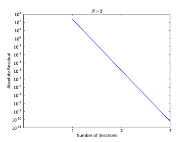
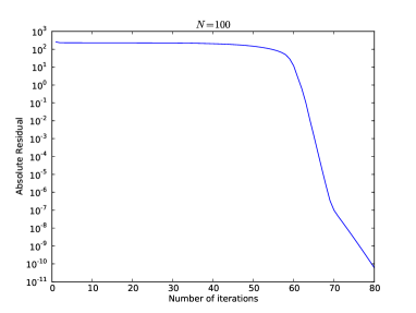
Refer to caption
Refer to caption
Figure 3: Convergence history, N=2,100𝑁2100N=2,100, 𝒱=x2𝒱superscript𝑥2\mathscr{V}=-x^{2}, Δt=0.001Δ𝑡0.001\Delta t=0.001, Δx=105Δ𝑥superscript105\Delta x=10^{-5}, Fixed point.
Table 1: Computation time in seconds, 𝒱=x2𝒱superscript𝑥2\mathscr{V}=-x^{2}, Δt=0.001Δ𝑡0.001\Delta t=0.001, Δx=105Δ𝑥superscript105\Delta x=10^{-5}, Fixed point.
N𝑁N 2 10 100 500
Trefsuperscript𝑇refT^{\mathrm{ref}} 403.56
Tclssuperscript𝑇clsT^{\mathrm{cls}} 773.07 2937.77 359.30 284.78
Tnewsuperscript𝑇newT^{\mathrm{new}} 773.72 178.30 18.19 4.76

Next, we use the Krylov methods (Gmres or Bicgstab) on the interface problem instead of the fixed point method. Table 2 present the computation time.

Table 2: Computation time in seconds, 𝒱=x2𝒱superscript𝑥2\mathscr{V}=-x^{2}, Δt=0.001Δ𝑡0.001\Delta t=0.001, Δx=105Δ𝑥superscript105\Delta x=10^{-5}, Gmres and Bicgstab.
N𝑁N 2 10 100 500 1000
Trefsuperscript𝑇refT^{\mathrm{ref}} 403.56
Gmres Tclssuperscript𝑇clsT^{\mathrm{cls}} 771.82 2577.51 2249.54 907.06 739.65
Tnewsuperscript𝑇newT^{\mathrm{new}} 777.42 177.20 18.95 6.86 8.17
Bicgstab Tclssuperscript𝑇clsT^{\mathrm{cls}} 774.19 2760.11 679.72 799.09 845.65
Tnewsuperscript𝑇newT^{\mathrm{new}} 774.44 177.02 18.18 6.83 7.12

As we can see, the use of Krylov methods allows to obtain robust scalable SWR algorithms. The algorithms converge for 1000 subdomains and are scalable up to 500 subdomains. Besides their computation times are lower than the ones of the classical algorithm. Roughly speaking, in Table 1 and Table 2 we have

Tcls=Tsub×Niter+,superscript𝑇clssubscript𝑇subsubscript𝑁iter\displaystyle T^{\mathrm{cls}}=T_{\mathrm{sub}}\times N_{\mathrm{iter}}+...,
Tnew=Tsub×4+TLd+,superscript𝑇newsubscript𝑇sub4subscript𝑇𝐿𝑑\displaystyle T^{\mathrm{new}}=T_{\mathrm{sub}}\times 4+T_{Ld}+...,

where Tsubsubscript𝑇subT_{\mathrm{sub}} is the computation time for solving the equation on one subdomain, TLdsubscript𝑇𝐿𝑑T_{Ld} is the computation time for solving the interface problem, “...” represent the negligible part of computation time such as the construction of matrices for the finite element method. If the number of subdomains N𝑁N is not so large, then TsubTLdmuch-greater-thansubscript𝑇subsubscript𝑇𝐿𝑑T_{\mathrm{sub}}\gg T_{Ld} and the minimum of Nitersubscript𝑁iterN_{\mathrm{iter}} is 3 in all our tests. If the number of subdomains N𝑁N is large, then TLdTsubsimilar-tosubscript𝑇𝐿𝑑subscript𝑇subT_{Ld}\sim T_{\mathrm{sub}} and Niter4much-greater-thansubscript𝑁iter4N_{\mathrm{iter}}\gg 4. It is for this reason that the new algorithm takes less computation time. However, as the number of subdomains increase, TLdsubscript𝑇𝐿𝑑T_{Ld} becomes larger. Thus, the new algorithm loses scalability if the number of subdomains is large.

In conclusion, the new algorithm with Krylov methods is robust and it takes much less computation time than the classical algorithm.

6.2 Comparison of classical and preconditioned algorithms

In this part, we are interested in observing the robustness, the computation time and the scalability of the preconditioned and non-preconditioned (classical) algorithms for time dependent potential 𝒱=5tx𝒱5𝑡𝑥\mathscr{V}=5tx and nonlinear potential 𝒱=|u|2𝒱superscript𝑢2\mathscr{V}=|u|^{2}. We denote by Npcsubscript𝑁pcN_{\mathrm{pc}} the number of iterations required to obtain convergence with the preconditioned algorithm and Tpcsubscript𝑇pcT_{\mathrm{pc}} the computation time of the preconditioned algorithm. The transmission condition used in this section is S02superscriptsubscript𝑆02S_{0}^{2}. We use the zero vector as the initial vector g0subscript𝑔0g_{0}.

First, we present in Figure 4 the convergence history for 𝒱=5tx𝒱5𝑡𝑥\mathscr{V}=5tx. If N𝑁N is not large, then there is no big difference between the classical algorithm and the preconditioned algorithm. However, if N𝑁N is large, then as at each iteration, one subdomain communicate only with two adjacent subdomains, we can see that the non-preconditioned algorithm converges very slowly in the first interations. The convergence of the preconditioned algorithm improves greatly since the preconditioner allows communication with remote subdomains.
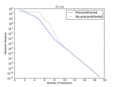
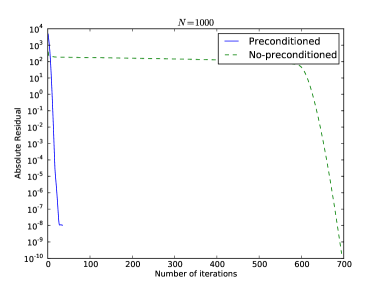
Refer to caption
Refer to caption
Figure 4: Convergence history, N=10,1000𝑁101000N=10,1000, 𝒱=5tx𝒱5𝑡𝑥\mathscr{V}=5tx, Δt=0.001Δ𝑡0.001\Delta t=0.001, Δx=105Δ𝑥superscript105\Delta x=10^{-5}.

The number of iterations required for convergence and the computation time are presented in Table 3 for N=10𝑁10N=10, N=100𝑁100N=100, N=500𝑁500N=500 and N=1000𝑁1000N=1000. We can see that the preconditioner allows to decrease significantly both the number of iterations and the computation time. The strong scalability of the classical algorithm is very low. Indeed, the number of iterations required increases with the number of subdomains. The preconditioned algorithm is much more scalable (up to 500 subdomains). However, it loses scalability from N=500𝑁500N=500 to N=1000𝑁1000N=1000. There are two reasons. One is that the number of iterations required for N=1000𝑁1000N=1000 is a little bit more than that for N=500𝑁500N=500. The other one is linked to the implementation of the preconditioner. Indeed, the time Tpcsubscript𝑇pcT_{\mathrm{pc}} consists of three major parts: the application of \mathcal{R} to vectors (step 1, denoted by T1subscript𝑇1T_{1}), the construction of the preconditioner (denoted by T3csubscript𝑇3𝑐T_{3c}) and the application of preconditioner (step 3, denoted by T3subscript𝑇3T_{3}). We have thereby

TpcT1+T3c+T3.subscript𝑇pcsubscript𝑇1subscript𝑇3𝑐subscript𝑇3T_{\mathrm{pc}}\approx T_{1}+T_{3c}+T_{3}. (32)

If N𝑁N is not very large, T1T3cT3similar-tosubscript𝑇1subscript𝑇3𝑐much-greater-thansubscript𝑇3T_{1}\sim T_{3c}\gg T_{3}. By increasing the number of subdomains, T1subscript𝑇1T_{1} and T3csubscript𝑇3𝑐T_{3c} decreases and T3subscript𝑇3T_{3} increases. Thus, if N𝑁N is large, T3subscript𝑇3T_{3} is not negligible compared to T1subscript𝑇1T_{1} and T3csubscript𝑇3𝑐T_{3c}. However, it is not very convenient to estimate T1subscript𝑇1T_{1} and T3subscript𝑇3T_{3} in our codes because we use the "free-matrix" solvers in the PETSc library. To confirm our explanation, we make tests using a coarser mesh in space (Δt=0.001Δ𝑡0.001\Delta t=0.001, Δx=104Δ𝑥superscript104\Delta x=10^{-4}). The size of the interface problem (13) is the same, thus T3subscript𝑇3T_{3} should be similar to that of the previous tests (Δt=0.001Δ𝑡0.001\Delta t=0.001, Δx=105Δ𝑥superscript105\Delta x=10^{-5}). But the size of the problem on a subdomain is ten times smaller. Thus, T1subscript𝑇1T_{1} and T3csubscript𝑇3𝑐T_{3c} are both smaller. The preconditioned algorithm should be less scalable. The results are shown in Table 4. It can be seen that the computation time Tpcsubscript𝑇pcT_{\mathrm{pc}} for N=1000𝑁1000N=1000 is larger than for N=500𝑁500N=500 and the preconditioned algorithm is not very scalable from N=100𝑁100N=100 to N=500𝑁500N=500. Despite this remark, we could conclude from our tests that the preconditioned algorithm reduces a lot the number of iterations and the computing time compared to the classical algorithm.

Table 3: Number of iterations required and computation time of the classical algorithm and the preconditioned algorithm, 𝒱=5tx𝒱5𝑡𝑥\mathscr{V}=5tx, Δt=0.001Δ𝑡0.001\Delta t=0.001, Δx=105Δ𝑥superscript105\Delta x=10^{-5}.
N𝑁N 10 100 500 1000
Nnopcsubscript𝑁nopcN_{\mathrm{nopc}} 17 71 349 695
Npcsubscript𝑁pcN_{\mathrm{pc}} 17 32 31 35
Trefsuperscript𝑇refT^{\mathrm{ref}} 6496.3
Tnopcsubscript𝑇nopcT_{\mathrm{nopc}} 10123.1 3217.0 2466.5 2238.0
Tpcsubscript𝑇pcT_{\mathrm{pc}} 10128.9 1432.7 250.0 170.7
Table 4: Number of iterations required and computation time of the classical algorithm and the preconditioned algorithm, 𝒱=5tx𝒱5𝑡𝑥\mathscr{V}=5tx, Δt=0.001Δ𝑡0.001\Delta t=0.001, Δx=104Δ𝑥superscript104\Delta x=10^{-4}.
N𝑁N 10 100 500 1000
Nnopcsubscript𝑁nopcN_{\mathrm{nopc}} 17 71 349 695
Npcsubscript𝑁pcN_{\mathrm{pc}} 17 32 26 25
Trefsuperscript𝑇refT^{\mathrm{ref}} 507.5
Tnopcsubscript𝑇nopcT_{\mathrm{nopc}} 681.9 223.8 210.2 191.2
Tpcsubscript𝑇pcT_{\mathrm{pc}} 694.3 107.6 38.4 54.5

Next, we reproduce the same tests for the nonlinear potential 𝒱=|u|2𝒱superscript𝑢2\mathscr{V}=|u|^{2}. The convergence history is presented in Figure 5. We show the number of iterations and the computation time in Table 5. The conclusions are quite similar.
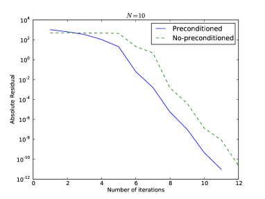
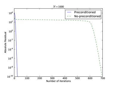
Refer to caption
Refer to caption
Figure 5: Convergence history, N=10,1000𝑁101000N=10,1000, 𝒱=|u|2𝒱superscript𝑢2\mathscr{V}=|u|^{2}, Δt=0.001Δ𝑡0.001\Delta t=0.001, Δx=105Δ𝑥superscript105\Delta x=10^{-5}.
Table 5: Number of iterations required and computation time of the classical algorithm and the preconditioned algorithm, 𝒱=|u|2𝒱superscript𝑢2\mathscr{V}=|u|^{2}, Δt=0.001Δ𝑡0.001\Delta t=0.001, Δx=105Δ𝑥superscript105\Delta x=10^{-5}.
N𝑁N 10 100 500 1000
Nnopcsubscript𝑁nopcN_{\mathrm{nopc}} 12 71 349 694
Npcsubscript𝑁pcN_{\mathrm{pc}} 11 22 25 26
Trefsuperscript𝑇refT^{\mathrm{ref}} 3200.8
Tnopcsubscript𝑇nopcT_{\mathrm{nopc}} 2582.3 1332.2 1248.0 1129.7
Tpcsubscript𝑇pcT_{\mathrm{pc}} 2446.7 408.2 117.6 83.8

6.3 Comparison of the transmission conditions

In this part, we compare the transmission conditions which are presented in Section 2 in the framework of the new algorithm for 𝒱=x2𝒱superscript𝑥2\mathscr{V}=-x^{2} and the preconditioned algorithm for 𝒱=|u|2𝒱superscript𝑢2\mathscr{V}=|u|^{2}. The theoretical optimal parameter p𝑝p in the transmission condition Robin being not at hand, we seek the best parameter numerically. We use in the subsection the random vector as the initial vector g0subscript𝑔0g_{0} to make sure that all frequencies are present.

6.3.1 Case of linear potential

We first consider the linear potential 𝒱=x2𝒱superscript𝑥2\mathscr{V}=-x^{2}. We compare the number of iterations, the total computation time to perform a complete simulation and the computation time required (TLdsubscript𝑇𝐿𝑑T_{Ld}) to solve the interface problem in Table 6 for N=2𝑁2N=2 using the fixed point method, Gmres and Bicgstab methods on the interface problem. As can be seen, the total computation times are almost identical. The required computation time for solving the interface problem is relatively close to zero compared with the total computation time. Therefore, we are interested rather in the number of iterations. We can make the following observations

  1. 1.

    the number of iterations required for the Robin transmission condition is greater compared to the other three strategies,

  2. 2.

    in each strategy, the number of iterations is not sensitive to order,

  3. 3.

    for the Padé approximation strategy, the number of iterations decrease as the parameter of Padé (m𝑚m) increase.

Table 6: Comparison of transmission conditions for N=2𝑁2N=2, V=x2𝑉superscript𝑥2V=-x^{2}, Δt=103Δ𝑡superscript103\Delta t=10^{-3}, Δx=105Δ𝑥superscript105\Delta x=10^{-5}.
Fixed point Gmres Bicgstab
Strategy Nitersubscript𝑁iterN_{\mathrm{iter}} TLdsubscript𝑇𝐿𝑑T_{Ld} Ttotalsubscript𝑇totalT_{\mathrm{total}} Nitersubscript𝑁iterN_{\mathrm{iter}} TLdsubscript𝑇𝐿𝑑T_{Ld} Ttotalsubscript𝑇totalT_{\mathrm{total}} Nitersubscript𝑁iterN_{\mathrm{iter}} TLdsubscript𝑇𝐿𝑑T_{Ld} Ttotalsubscript𝑇totalT_{\mathrm{total}}
S0Msuperscriptsubscript𝑆0𝑀S_{0}^{M} S02superscriptsubscript𝑆02S_{0}^{2} 6 0.005 775.7 5 0.002 774.2 3 0.002 773.8
S03superscriptsubscript𝑆03S_{0}^{3} 6 0.002 774.2 5 0.002 779.6 3 0.002 773.3
S04superscriptsubscript𝑆04S_{0}^{4} 6 0.002 769.0 5 0.002 774.2 3 0.002 773.6
S1Msuperscriptsubscript𝑆1𝑀S_{1}^{M} S12superscriptsubscript𝑆12S_{1}^{2} 6 0.002 773.4 5 0.002 773.2 3 0.002 773.8
S14superscriptsubscript𝑆14S_{1}^{4} 6 0.002 773.9 5 0.002 773.6 3 0.002 774.5
S2Msuperscriptsubscript𝑆2𝑀S_{2}^{M} S22,20superscriptsubscript𝑆2220S_{2}^{2,20} 191 0.062 773.3 28 0.010 774.5 16 0.011 773.1
S22,50superscriptsubscript𝑆2250S_{2}^{2,50} 76 0.025 773.6 27 0.010 773.3 15 0.010 773.6
S22,100superscriptsubscript𝑆22100S_{2}^{2,100} 39 0.013 776.3 23 0.008 775.2 13 0.009 773.6
S24,20superscriptsubscript𝑆2420S_{2}^{4,20} 181 0.059 769.9 28 0.010 774.6 15 0.010 773.6
S24,50superscriptsubscript𝑆2450S_{2}^{4,50} 77 0.025 776.0 27 0.010 773.5 15 0.010 773.3
S24,100superscriptsubscript𝑆24100S_{2}^{4,100} 39 0.013 775.4 23 0.008 773.8 13 0.009 774.8
Robin 1112 0.360 774.7 47 0.017 776.4 27 0.018 777.4
  • 1.

    * the parameters for the transmission condition Robin are p=44𝑝44p=44 (fixed point), p=5𝑝5p=5 (Gmres) and p=5𝑝5p=5 (Bicgstab).

We make the same tests for N=500𝑁500N=500, the results are shown in Table 7. We could see that

  1. 1.

    in each strategy, the number of iterations is not sensitive to order,

  2. 2.

    for the Padé approximation strategy, if the parameter m𝑚m is small, then the algorithm is not robust,

  3. 3.

    the Krylov methods (Gmres and Bicgstab) could not always reduce the number of iterations.

Table 7: Comparison of transmission conditions for N=500𝑁500N=500, V=x2𝑉superscript𝑥2V=-x^{2}, Δt=103Δ𝑡superscript103\Delta t=10^{-3}, Δx=105Δ𝑥superscript105\Delta x=10^{-5}.
Fixed point Gmres Bicgstab
Strategy Nitersubscript𝑁iterN_{\mathrm{iter}} TLdsubscript𝑇𝐿𝑑T_{Ld} Ttotalsubscript𝑇totalT_{\mathrm{total}} Nitersubscript𝑁iterN_{\mathrm{iter}} TLdsubscript𝑇𝐿𝑑T_{Ld} Ttotalsubscript𝑇totalT_{\mathrm{total}} Nitersubscript𝑁iterN_{\mathrm{iter}} TLdsubscript𝑇𝐿𝑑T_{Ld} Ttotalsubscript𝑇totalT_{\mathrm{total}}
S0Msuperscriptsubscript𝑆0𝑀S_{0}^{M} S02superscriptsubscript𝑆02S_{0}^{2} 357 0.775 4.68 1023 2.883 6.91 368 1.646 5.51
S03superscriptsubscript𝑆03S_{0}^{3} 337 0.734 4.62 977 2.620 6.55 345 1.831 5.77
S04superscriptsubscript𝑆04S_{0}^{4} 337 0.733 4.65 978 2.681 6.54 350 1.739 5.73
S1Msuperscriptsubscript𝑆1𝑀S_{1}^{M} S12superscriptsubscript𝑆12S_{1}^{2} 341 0.745 4.62 1010 2.364 6.20 353 2.102 6.00
S14superscriptsubscript𝑆14S_{1}^{4} 340 0.743 4.63 1023 3.454 7.19 351 2.225 6.06
S2Msuperscriptsubscript𝑆2𝑀S_{2}^{M} S22,20superscriptsubscript𝑆2220S_{2}^{2,20} - 1240 3.368 7.34 440 2.626 6.64
S22,50superscriptsubscript𝑆2250S_{2}^{2,50} - 997 2.320 6.30 352 2.240 6.16
S22,100superscriptsubscript𝑆22100S_{2}^{2,100} 336 0.735 4.62 998 3.055 7.03 333 1.603 5.62
S24,20superscriptsubscript𝑆2420S_{2}^{4,20} - 1216 3.349 7.31 464 2.044 6.05
S24,50superscriptsubscript𝑆2450S_{2}^{4,50} - 1043 3.907 7.85 336 1.756 5.63
S24,100superscriptsubscript𝑆24100S_{2}^{4,100} 336 0.733 4.60 1024 2.424 6.35 334 1.989 5.95
Robin 1690 3.628 7.52 1060 3.000 6.80 318 1.41 5.32
  • 1.

    *: the parameters for the transmission condition Robin are p=45𝑝45p=45 (fixed point), p=19𝑝19p=19 (Gmres) and p=6𝑝6p=6 (Bicgstab).

  • 2.

    -: the algorithm does not converge before 2000 iterations.

We could conclude that if the number of subdomains N𝑁N is not very large, the potential strategy in order 2 with Bicgstab method on the interface problem is a good choice. If N𝑁N is large, the Bicgstab method also allows most of the algorithms to converge, but it is difficult to have a general conclusion for the transmission conditions in the framework of new algorithm.

6.3.2 Case of nonlinear potential

Now we turn to compare the transmission conditions for the nonlinear potential 𝒱=|u|2𝒱superscript𝑢2\mathscr{V}=|u|^{2} in the framework of the preconditioned algorithm. First, we study the influence of the parameter p𝑝p in the Robin transmission condition. The number of iterations and the computation time are shown in Table 8. It is clear that the convergence is not sensitive to this parameter.

Table 8: Influence of parameter p𝑝p in the transmission conditions Robin, N=2,10,100𝑁210100N=2,10,100, 𝒱=|u|2𝒱superscript𝑢2\mathscr{V}=|u|^{2}, Δt=0.001Δ𝑡0.001\Delta t=0.001, Δx=104Δ𝑥superscript104\Delta x=10^{-4}.
Robin N=2𝑁2N=2 N=10𝑁10N=10 N=100𝑁100N=100
p𝑝p Nitersubscript𝑁iterN_{\mathrm{iter}} Ttotalsubscript𝑇totalT_{\mathrm{total}} Nitersubscript𝑁iterN_{\mathrm{iter}} Ttotalsubscript𝑇totalT_{\mathrm{total}} Nitersubscript𝑁iterN_{\mathrm{iter}} Ttotalsubscript𝑇totalT_{\mathrm{total}}
555 9 1042.6 12 257.9 21 55.7
101010 8 920.3 11 230.9 22 50.6
151515 8 920.3 11 228.7 22 46.7
202020 8 914.5 11 226.1 22 43.7
252525 8 913.0 11 226.4 22 43.6
303030 8 919.2 11 227.6 22 43.9
353535 8 922.1 11 231.8 22 44.4
404040 8 922.8 12 250.2 22 45.0
454545 8 921.7 12 252.5 22 46.0
505050 8 928.3 12 253.3 22 46.7

Next we compare the three strategies. The numericals results are presented in Table 9. The transmission conditions S04superscriptsubscript𝑆04S_{0}^{4}, S14superscriptsubscript𝑆14S_{1}^{4} and S24superscriptsubscript𝑆24S_{2}^{4} include the evaluation of f(u)𝑓𝑢f(u). We don’t find a suitable discretization of this term such that the continuity of 𝐯jsubscript𝐯𝑗\mathbf{v}_{j} at the interfaces ensure the continuity of 𝐧jf(u)subscriptsubscript𝐧𝑗𝑓𝑢\partial_{\mathbf{n}_{j}}f(u). Thus we could not obtain the solution 𝐮j,nsubscript𝐮𝑗𝑛\mathbf{u}_{j,n} that satisfy 𝐮j,n=Rj𝐮0,nsubscript𝐮𝑗𝑛subscript𝑅𝑗subscript𝐮0𝑛\mathbf{u}_{j,n}=R_{j}\mathbf{u}_{0,n}. We could see that the number of iterations is not sensitive to the transmission condition and its order. However the computation time for the Padé strategy is greater than other strategies. On each subdomain, the non linearity is approximated by a fixed point procedure (see formula (12)). This fixed point procedure converges more slowly using the Padé strategy than the other strategies. This observation is also found in [14]. In conclusion, in the nonlinear case, we also think that the potential strategy of order 2 (S02superscriptsubscript𝑆02S_{0}^{2}) is a good choice.

Table 9: Comparison of transmission conditions for N=2,10,100𝑁210100N=2,10,100, 𝒱=|u|2𝒱superscript𝑢2\mathscr{V}=|u|^{2}, Δt=0.001Δ𝑡0.001\Delta t=0.001, Δx=104Δ𝑥superscript104\Delta x=10^{-4}.
N=2𝑁2N=2 N=10𝑁10N=10 N=100𝑁100N=100
Nitersubscript𝑁iterN_{\mathrm{iter}} Ttotalsubscript𝑇totalT_{\mathrm{total}} Nitersubscript𝑁iterN_{\mathrm{iter}} Ttotalsubscript𝑇totalT_{\mathrm{total}} Nitersubscript𝑁iterN_{\mathrm{iter}} Ttotalsubscript𝑇totalT_{\mathrm{total}}
S0Msuperscriptsubscript𝑆0𝑀S_{0}^{M} S02superscriptsubscript𝑆02S_{0}^{2} 8 909.5 11 229.1 22 40.6
S03superscriptsubscript𝑆03S_{0}^{3} 7 802.1 10 205.8 22 41.6
S1Msuperscriptsubscript𝑆1𝑀S_{1}^{M} S12superscriptsubscript𝑆12S_{1}^{2} 7 802.3 10 205.6 22 41.4
S2Msuperscriptsubscript𝑆2𝑀S_{2}^{M} S22,20superscriptsubscript𝑆2220S_{2}^{2,20} 7 1732.5 10 572.0 22 128.6
S22,50superscriptsubscript𝑆2250S_{2}^{2,50} 7 4042.9 10 1342.3 23 310.3
S22,100superscriptsubscript𝑆22100S_{2}^{2,100} 7 7900.5 10 2640.0 22 576.0
Remark 1

As we indicated previously, we explain here our choice of transmission condition: the potential strategy of order 2 (S02superscriptsubscript𝑆02S_{0}^{2}). Indeed, it seems reasonable to consider it since

  1. 1.

    the algorithm is robust and the computation time for S02superscriptsubscript𝑆02S_{0}^{2} is similar to others transmission conditions,

  2. 2.

    if N𝑁N is not so large, it is one of the best choice,

  3. 3.

    the implementation of S02superscriptsubscript𝑆02S_{0}^{2} is much easier than other transmission conditions.

6.4 Gpu acceleration

If the number of subdomain N𝑁N is not so large, then solving the Schrodinger equation on subdomains takes most of the computation time. We move these computations from Cpu to Gpu. In this subsection, we present the numerical experiments of Gpu acceleration. Two Gpu libraries of NVIDIA are used: CUSPARSE (tri-diagonal solver) and CUBLAS (BLAS operations). We use 8 Gpu Kepler K20, and compare the Cpu and Gpu results for N=2,4,8𝑁248N=2,4,8. We use always 1 Gpu/MPI process.

Table 10: Cpu and Gpu computation time, Bicgstab, S02superscriptsubscript𝑆02S_{0}^{2}, Δt=0.001Δ𝑡0.001\Delta t=0.001, Δx=105Δ𝑥superscript105\Delta x=10^{-5}, V=x2𝑉superscript𝑥2V=-x^{2}.
N𝑁N 2 4 8
TCpusuperscript𝑇CpuT^{\mathrm{Cpu}} 774.4 393.0 203.2
TGpusuperscript𝑇GpuT^{\mathrm{Gpu}} 27.90 16.13 12.54
TCpu/TGpusuperscript𝑇Cpusuperscript𝑇GpuT^{\mathrm{Cpu}}/T^{\mathrm{Gpu}} 18 24 16

Gpu could accelerate a lot the computation as shown in Table 10. However the algorithm on Gpu is not scalable. The reason is that the size of problem is not large enough for Gpu. Gpu waste some of its ability. We test a larger case only for Gpu: Δt=0.001Δ𝑡0.001\Delta t=0.001, Δx=106Δ𝑥superscript106\Delta x=10^{-6}. The results are shown in Table 11.

Table 11: Gpu computation time, Bicgstab, S02superscriptsubscript𝑆02S_{0}^{2}, Δ=0.001Δ0.001\Delta=0.001, Δx=5×10⁶Δ𝑥5superscript106\Delta x=5\times 10^{-6}, V=x2𝑉superscript𝑥2V=-x^{2}.
N𝑁N 2 4 8
TGpusuperscript𝑇GpuT^{\mathrm{Gpu}} 51.95 28.21 16.30

Finally, we make the same tests for the nonlinear potential in the framework of the preconditioned algorithm. The results are presented in Table 12 and Table 13. The conclusion is similar.

Table 12: Cpu and Gpu computation time, Δt=0.01Δ𝑡0.01\Delta t=0.01, Δx=105Δ𝑥superscript105\Delta x=10^{-5}, V=|u|2𝑉superscript𝑢2V=|u|^{2}.
N𝑁N 2 4 8
TCpusuperscript𝑇CpuT^{\mathrm{Cpu}} 373.6 526.7 316.0
TGpusuperscript𝑇GpuT^{\mathrm{Gpu}} 73.9 40.1 34.0
TCpu/TGpusuperscript𝑇Cpusuperscript𝑇GpuT^{\mathrm{Cpu}}/T^{\mathrm{Gpu}} 5 13 9
Table 13: Gpu computation time, Δt=0.01Δ𝑡0.01\Delta t=0.01, Δx=5×10⁶Δ𝑥5superscript106\Delta x=5\times 10^{-6}, V=|u|2𝑉superscript𝑢2V=|u|^{2}.
N𝑁N 2 4 8
TGpusuperscript𝑇GpuT^{\mathrm{Gpu}} 134.3 73.7 46.0

7 Conclusion

We proposed in this paper a new algorithm of the SWR method for the one dimensional Schrödinger equation with time independent linear potential and a preconditioned algorithm for general potentials. The algorithms for both cases are scalable and could reduce significantly the computation time. Some newly constructed absorbing boundary conditions are used as the transmission condition and compared numerically in the framework of the algorithms proposed by us. We believe that the potential strategy of order 2 is a good choice. Besides, we adapted the codes developed on Cpu to Gpu. According to the experiments, the computation could be accelerated obviously.

Acknowledgements

We acknowledge Pierre Kestener (Maison de la Simulation Saclay France) for the discussions about the parallel programming, especially for his help about Gpu acceleration. This work was partially supported by the French ANR grant ANR-12-MONU-0007-02 BECASIM (Modèles Numériques call).

References

References

  • [1] L. Halpern, J. Szeftel, Optimized and quasi-optimal Schwarz waveform relaxation for the one dimensional Schrödinger equation, Math. Model. Methods Appl. Sci. 20 (12) (2010) 2167–2199.
  • [2] L. Halpern, J. Szeftel, Optimized and quasi-optimal Schwarz waveform relaxation for the one-dimensional Schrödinger equation, Tech. rep., CNRS (2006).
  • [3] F. Caetano, M. J. Gander, L. Halpern, J. Szeftel, Schwarz waveform relaxation algorithms for semilinear reaction-diffusion equations, Networks Heterog. Media 5 (3) (2010) 487–505.
  • [4] M. J. Gander, L. Halpern, Optimized Schwarz Waveform Relaxation Methods for Advection Reaction Diffusion Problems, SIAM J. Numer. Anal. 45 (2) (2007) 666–697.
  • [5] T. Hoang, J. Jaffré, C. Japhet, M. Kern, J. Roberts, Space-Time Domain Decomposition Methods for Diffusion Problems in Mixed Formulations 51 (6) (2013) 3532–3559.
  • [6] M. J. Gander, L. Halpern, F. Nataf, Optimal Schwarz waveform relaxation for the one dimensional wave equation, SIAM J. Numer. Anal. 41 (5) (2003) 1643–1681.
  • [7] L. Halpern, J. Szeftel, Nonlinear nonoverlapping Schwarz waveform relaxation for semilinear wave propagation, Math. Comput. 78 (266) (2009) 865–889.
  • [8] V. Dolean, M. J. Gander, L. Gerardo-Giorda, Optimized Schwarz Methods for Maxwell’s Equations, SIAM J. Sci. Comput. 31 (3) (2009) 2193–2213.
  • [9] X. Antoine, E. Lorin, A. D. Bandrauk, Domain Decomposition Methods and High-Order Absorbing Boundary Conditions for the Numerical Simulation of the Time Dependent Schrödinger Equation with Ionization and Recombination by Intense Electric Field.
  • [10] X. Antoine, C. Besse, S. Descombes, Artificial boundary conditions for one-dimensional cubic nonlinear Schrödinger equations, SIAM J. Numer. Anal. 43 (6) (2006) 2272–2293.
  • [11] X. Antoine, C. Besse, P. Klein, Absorbing boundary conditions for the one-dimensional Schrödinger equation with an exterior repulsive potential, J. Comput. Phys. 228 (2) (2009) 312–335.
  • [12] X. Antoine, C. Besse, P. Klein, Absorbing Boundary Conditions for General Nonlinear Schrödinger Equations, SIAM J. Sci. Comput. 33 (2) (2011) 1008–1033.
  • [13] X. Antoine, C. Besse, J. Szeftel, Towards accurate artificial boundary conditions for nonlinear PDEs through examples, Cubo, A Math. J. 11 (4) (2009) 29–48.
  • [14] P. Klein, Construction et analyse de conditions aux limites artificielles pour des équations de Schrödinger avec potentiels et non linéarités, Ph.D. thesis, Université Henri Poincaré, Nancy 1 (2010).
  • [15] A. Durán, J. Sanz-Serna, The numerical integration of relative equilibrium solutions. The nonlinear Schrodinger equation, IMA J. Numer. Anal. 20 (2) (2000) 235–261.
  • [16] Y. Saad, Iterative methods for sparse linear systems, 2nd Edition, Society for Industrial and Applied Mathematics, 2003.
  • [17] S. Balay, M. F. Adams, J. Brown, P. Brune, K. Buschelman, V. Eijkhout, W. D. Gropp, D. Kaushik, M. G. Knepley, L. C. McInnes, K. Rupp, B. F. Smith, H. Zhang, PETSc Users Manual, Tech. Rep. ANL-95/11 - Revision 3.4, Argonne National Laboratory (2013).
  • [18] Message Passing Interface Forum, MPI : A Message-Passing Interface Standard Version 3.0, Tech. rep. (2012).
  • [19] M. J. Gander, Schwarz methods over the course of time, Electron. Trans. Numer. Anal. 31 (2008) 228–255.