Kernel-Based Just-In-Time Learning for
Passing Expectation Propagation Messages

Abstract

We propose an efficient nonparametric strategy for learning a message operator in expectation propagation (EP), which takes as input the set of incoming messages to a factor node, and produces an outgoing message as output. This learned operator replaces the multivariate integral required in classical EP, which may not have an analytic expression. We use kernel-based regression, which is trained on a set of probability distributions representing the incoming messages, and the associated outgoing messages. The kernel approach has two main advantages: first, it is fast, as it is implemented using a novel two-layer random feature representation of the input message distributions; second, it has principled uncertainty estimates, and can be cheaply updated online, meaning it can request and incorporate new training data when it encounters inputs on which it is uncertain. In experiments, our approach is able to solve learning problems where a single message operator is required for multiple, substantially different data sets (logistic regression for a variety of classification problems), where it is essential to accurately assess uncertainty and to efficiently and robustly update the message operator.

1 INTRODUCTION

An increasing priority in Bayesian modelling is to make inference accessible and implementable for practitioners, without requiring specialist knowledge. This is a goal sought, for instance, in probabilistic programming languages (Wingate et al., 2011; Goodman et al., 2008), as well as in more granular, component-based systems (Stan Development Team, 2014; Minka et al., 2014). In all cases, the user should be able to freely specify what they wish their model to express, without having to deal with the complexities of sampling, variational approximation, or distribution conjugacy. In reality, however, model convenience and simplicity can limit or undermine intended models, sometimes in ways the users might not expect. To take one example, the inverse gamma prior, which is widely used as a convenient conjugate prior for the variance, has quite pathological behaviour (Gelman, 2006). In general, more expressive, freely chosen models are more likely to require expensive sampling or quadrature approaches, which can make them challenging to implement or impractical to run.

We address the particular setting of expectation propagation (Minka, 2001), a message passing algorithm wherein messages are confined to being members of a particular parametric family. The process of integrating incoming messages over a factor potential, and projecting the result onto the required output family, can be difficult, and in some cases not achievable in closed form. Thus, a number of approaches have been proposed to implement EP updates numerically, independent of the details of the factor potential being used. One approach, due to Barthelmé and Chopin (2011), is to compute the message update via importance sampling. While these estimates converge to the desired integrals for a sufficient number of importance samples, the sampling procedure must be run at every iteration during inference, hence it is not viable for large-scale problems.

An improvement on this approach is to use importance sampled instances of input/output message pairs to train a regression algorithm, which can then be used in place of the sampler. Heess et al. (2013) use neural networks to learn the mapping from incoming to outgoing messages, and the learned mappings perform well on a variety of practical problems. This approach comes with a disadvantage: it requires training data that cover the entire set of possible input messages for a given type of problem (e.g., datasets representative of all classification problems the user proposes to solve), and it has no way of assessing the uncertainty of its prediction, or of updating the model online in the event that a prediction is uncertain.

The disadvantages of the neural network approach were the basis for work by Eslami et al. (2014), who replaced the neural networks with random forests. The random forests provide uncertainty estimates for each prediction. This allows them to be trained ‘just-in-time’, during EP inference, whenever the predictor decides it is uncertain. Uncertainty estimation for random forests relies on unproven heuristics, however: we demonstrate empirically that such heuristics can become highly misleading as we move away from the initial training data. Moreover, online updating can result in unbalanced trees, resulting in a cost of prediction of $O(N)$ for training data of size $N$, rather than the ideal of $O(\log(N))$.

We propose a novel, kernel-based approach to learning a message operator nonparametrically for expectation propagation. The learning algorithm takes the form of a distribution regression problem, where the inputs are probability measures represented as embeddings of the distributions to a reproducing kernel Hilbert space (RKHS), and the outputs are vectors of message parameters (Szabó et al., 2014). A first advantage of this approach is that one does not need to pre-specify customized features of the distributions, as in (Eslami et al., 2014; Heess et al., 2013). Rather, we use a general characteristic kernel on input distributions (Christmann and Steinwart, 2010, eq. 9). To make the algorithm computationally tractable, we regress directly in the primal from random Fourier features of the data (Rahimi and Recht, 2007; Le et al., 2013; Yang et al., 2015). In particular, we establish a novel random feature representation for when inputs are distributions, via a two-level random feature approach. This gives us both fast prediction (linear in the number of random features), and fast online updates (quadratic in the number of random features).

A second advantage of our approach is that, being an instance of Gaussian process regression, there are well established estimates of predictive uncertainty (Rasmussen and Williams, 2006, Ch. 2). We use these uncertainty estimates so as to determine when to query the importance sampler for additional input/output pairs, i.e., the uncertain predictions trigger just-in-time updates of the regressor. We demonstrate empirically that our uncertainty estimates are more robust and informative than those for random forests, especially as we move away from the training data.

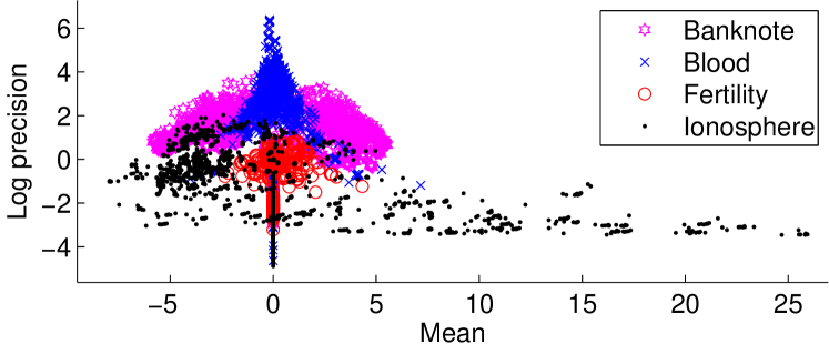
Figure 1: Distributions of incoming messages to logistic factor in four different UCI datasets.

Our paper proceeds as follows. In Section 2, we introduce the notation for expectation propagation, and indicate how an importance sampling procedure can be used as an oracle to provide training data for the message operator. We also give a brief overview of previous learning approaches to the problem, with a focus on that of Eslami et al. (2014). Next, in Section 3, we describe our kernel regression approach, and the form of an efficient kernel message operator mapping the input messages (distributions embedded in an RKHS) to outgoing messages (sets of parameters of the outgoing messages). Finally, in Section 4, we describe our experiments, which cover three topics: a benchmark of our uncertainty estimates, a demonstration of factor learning on artificial data with well-controlled statistical properties, and a logistic regression experiment on four different real-world datasets, demonstrating that our just-in-time learner can correctly evaluate its uncertainty and update the regression function as the incoming messages change (see Fig. 1). Code to implement our method is available online at https://github.com/wittawatj/kernel-ep.

2 BACKGROUND

We assume that distributions (or densities) $p$ over a set of variables $\mathbf{x}=(x_{1},\dots x_{d})$ of interest can be represented as factor graphs, i.e. $p(\mathbf{x})=\frac{1}{Z}\prod_{j=1}^{J}f_{j}(\mathbf{x}_{\mathrm{ne}(f_{j})})$. The factors $f_{j}$ are non-negative functions which are defined over subsets $\mathbf{x}_{\mathrm{ne}(f_{j})}$ of the full set of variables $\mathbf{x}$. These variables form the neighbors of the factor node $f_{j}$ in the factor graph, and we use $\mathrm{ne}(f_{j})$ to denote the corresponding set of indices. $Z$ is the normalization constant.

We deal with models in which some of the factors have a non-standard form, or may not have a known analytic expression (i.e. “black box” factors). Although our approach applies to any such factor in principle, in this paper we focus on directed factors $f(\mathbf{x}_{\mathrm{out}}|\mathbf{x}_{\mathrm{in}})$ which specify a conditional distribution over variables $\mathbf{x}_{\mathrm{out}}$ given $\mathbf{x}_{\mathrm{in}}$ (and thus $\mathbf{x}_{\mathrm{ne}(f)}=(\mathbf{x}_{\mathrm{out}},\mathbf{x}_{\mathrm{in}}))$. The only assumption we make is that we are provided with a forward sampling function $f:\mathbf{x}_{\mathrm{in}}\mapsto\mathbf{x}_{\mathrm{out}}$, i.e., a function that maps (stochastically or deterministically) a setting of the input variables $\mathbf{x}_{\mathrm{in}}$ to a sample from the conditional distribution over $\mathbf{x}_{\mathrm{out}}\sim f(\cdot|\mathbf{x}_{\mathrm{in}})$. In particular, the ability to evaluate the value of $f(\mathbf{x}_{\mathrm{out}}|\mathbf{x}_{\mathrm{in}})$ is not assumed. A natural way to specify $f$ is as code in a probabilistic program.

2.1 EXPECTATION PROPAGATION

Expectation Propagation (EP) is an approximate iterative procedure for computing marginal beliefs of variables by iteratively passing messages between variables and factors until convergence (Minka, 2001). It can be seen as an alternative to belief propagation, where the marginals are projected onto a member of some class of known parametric distributions. The message $m_{f\rightarrow V}(x_{V})$ from factor $f$ to variable $V\in\mathrm{ne}(f)$ is

$$\frac{\mathrm{proj}\left[\int f(\mathbf{x}_{\mathrm{ne}(f)})\prod_{V^{\prime}\in\mathrm{ne}(f)}m_{V^{\prime}\rightarrow f}(x_{V^{\prime}})\mathrm{d}\mathbf{x}_{\mathrm{ne}(f)\backslash V}\right]}{m_{V\rightarrow f}(x_{V})},$$ (1)

where $m_{V^{\prime}\rightarrow f}$ are the messages sent to factor $f$ from all of its neighboring variables $x_{V^{\prime}}$, $\mathrm{proj}\left[p\right]=\mathrm{arg}\mathrm{min}_{q\in\mathcal{Q}}\mathrm{KL}\left[p||q\right]$, and $\mathcal{Q}$ is typically in the exponential family, e.g. the set of Gaussian or Beta distributions.

Computing the numerator of (1) can be challenging, as it requires evaluating a high-dimensional integral as well as minimization of the Kullback-Leibler divergence to some non-standard distribution. Even for factors with known analytic form this often requires hand-crafted approximations, or the use of expensive numerical integration techniques; for “black-box” factors implemented as forward sampling functions, fully nonparametric techniques are needed.

Barthelmé and Chopin (2011); Heess et al. (2013); Eslami et al. (2014) propose an alternative, stochastic approach to the integration and projection step. When the projection is to a member $q(x|\eta)=h(x)\exp\left(\eta^{\top}u(x)-A(\eta)\right)$ of an exponential family, one simply computes the expectation of the sufficient statistic $u(\cdot)$ under the numerator of (1). A sample based approximation of this expectation can be obtained via Monte Carlo simulation. Given a forward-sampling function $f$ as described above, one especially simple approach is importance sampling,

$$\mathbb{E}_{\mathbf{x}_{\mathrm{ne}(f)}\sim b}\left[u(x_{V})\right] \approx\frac{1}{M}\sum_{l=1}^{M}w(\mathbf{x}_{\mathrm{ne}(f)}^{l})u(x_{V}^{l}),$$ (2)

where $\mathbf{x}_{\mathrm{ne}(f)}^{l}\sim\tilde{b}$, for $l=1,\ldots,M$ and on the left hand side,

$$b(\mathbf{x}_{\mathrm{ne}(f)})=f(\mathbf{x}_{\mathrm{ne}(f)})\prod_{W\in\mathrm{ne}(f)}m_{W\rightarrow f}(x_{W}).$$

On the right hand side we draw samples $\mathbf{x}_{\mathrm{ne}(f)}^{l}$ from some proposal distribution $\tilde{b}$ which we choose to be $\tilde{b}(\mathbf{x}_{\mathrm{ne}(f)})=r(\mathbf{x}_{\mathrm{in}})f(\mathbf{x}_{\mathrm{out}}|\mathbf{x}_{\mathrm{in}})$ for some distribution $r$ with appropriate support, and compute importance weights

$$w(\mathbf{x}_{\mathrm{ne}(f)})=\frac{\prod_{W\in\mathrm{ne}(f)}m_{W\rightarrow f}(x_{W})}{r(\mathbf{x}_{\mathrm{in}})}.$$

Thus the estimated expected sufficient statistics provide us with an estimate of the parameters $\eta$ of the result $q$ of the projection $\mathrm{proj}\left[p\right]$, from which the message is readily computed.

2.2 JUST-IN-TIME LEARNING OF MESSAGES

Message approximations as in the previous section could be used directly when running the EP algorithm, as in Barthelmé and Chopin (2011), but this approach can suffer when the number of samples $M$ is small, and the importance sampling estimate is not reliable. On the other hand, for large $M$ the computational cost of running EP with approximate messages can be very high, as importance sampling must be performed for sending each outgoing message. To obtain low-variance message approximations at lower computational cost, Heess et al. (2013) and Eslami et al. (2014) both amortize previously computed approximate messages by training a function approximator to directly map a tuple of incoming variable-to-factor messages $(m_{V^{\prime}\rightarrow f})_{V^{\prime}\in\mathrm{ne}(f)}$ to an approximate factor to variable message $m_{f\rightarrow V}$, i.e.  they learn a mapping

$$M_{f\rightarrow V}^{\theta}:(m_{V^{\prime}\rightarrow f})_{V^{\prime}\in\mathrm{ne}(f)}\mapsto m_{f\rightarrow V},$$ (3)

where $\theta$ are the parameters of the approximator.

Heess et al. (2013) use neural networks and a large, fixed training set to learn their approximate message operator prior to running EP. By contrast, Eslami et al. (2014) employ random forests as their class of learning functions, and update their approximate message operator on the fly during inference, depending on the predictive uncertainty of the current message operator. Specifically, they endow their function approximator with an uncertainty estimate

$${\mathfrak{V}}_{f\rightarrow V}^{\theta}:(m_{V^{\prime}\rightarrow f})_{V^{\prime}\in\mathrm{ne}(f)}\mapsto{\mathfrak{v}},$$ (4)

where ${\mathfrak{v}}$ indicates the expected unreliability of the predicted, approximate message $m_{f\rightarrow V}$ returned by $M_{f\rightarrow V}^{\theta}$. If ${\mathfrak{v}}={\mathfrak{V}}_{f\rightarrow V}^{\theta}\left((m_{V^{\prime}\rightarrow f})_{V^{\prime}\in\mathrm{ne}(f)}\right)$ exceeds a pre-defined threshold, the required message is approximated via importance sampling (cf. (2)) and $M_{f\rightarrow V}^{\theta}$ is updated on this new datapoint (leading to a new set of parameters $\theta^{\prime}$ with ${\mathfrak{V}}_{f\rightarrow V}^{\theta^{\prime}}\left((m_{V^{\prime}\rightarrow f})_{V^{\prime}\in\mathrm{ne}(f)}\right))<{\mathfrak{V}}_{f\rightarrow V}^{\theta}\left((m_{V^{\prime}\rightarrow f})_{V^{\prime}\in\mathrm{ne}(f)}\right)$.

Eslami et al. (2014) estimate the predictive uncertainty ${\mathfrak{V}}_{f\rightarrow V}^{\theta}$ via the heuristic of looking at the variability of the forest predictions for each point (Criminisi and Shotton, 2013). They implement their online updates by splitting the trees at their leaves. Both these mechanisms can be problematic, however. First, the heuristic used in computing uncertainty has no guarantees: indeed, uncertainty estimation for random forests remains a challenging topic of current research (Hutter, 2009). This is not merely a theoretical consideration: in our experiments in Section 4, we demonstrate that uncertainty heuristics for random forests become unstable and inaccurate as we move away from the initial training data. Second, online updates of random forests may not work well when the newly observed data are from a very different distribution to the initial training sample (e.g. Lakshminarayanan et al., 2014, Fig. 3). For large amounts of training set drift, the leaf-splitting approach of Eslami et al. can result in a decision tree in the form of a long chain, giving a worst case cost of prediction (computational and storage) of $O(N)$ for training data of size $N$, vs the ideal of $O(\log(N))$ for balanced trees. Finally, note that the approach of Eslami et al. uses certain bespoke features of the factors when specifying tree traversal in the random forests, notably the value of the factor potentials at the mean and mode of the incoming messages. These features require expert knowledge of the model on the part of the practitioner, and are not available in the “forward sampling” setting. The present work does not employ such features.

In terms of computational cost, prediction for the random forest of Eslami et al. costs $O(KD_{r}D_{t}\log(N))$, and updating following a new observation costs $O(KD_{r}^{3}D_{t}\log(N))$, where $K$ is the number of trees in the random forest, $D_{t}$ is the number of features used in tree traversal, $D_{r}$ is the number of features used in making predictions at the leaves, and $N$ is the number of training messages. Representative values are $K=64$, $D_{t}=D_{r}\approx 15$, and $N$ in the range of 1,000 to 5,000.

3 KERNEL LEARNING OF OPERATORS

We now propose a kernel regression method for jointly learning the message operator $M_{f\rightarrow V}^{\theta}$ and uncertainty estimate ${\mathfrak{V}}_{f\rightarrow V}^{\theta}$. We regress from the tuple of incoming messages, which are probability distributions, to the parameters of the outgoing message. To this end we apply a kernel over distributions from (Christmann and Steinwart, 2010) to the case where the input consists of more than one distribution.

We note that Song et al. (2010, 2011) propose a related regression approach for predicting outgoing messages from incoming messages, for the purpose of belief propagation. Their setting is different from ours, however, as their messages are smoothed conditional density functions rather than parametric distributions of known form.

To achieve fast predictions and factor updates, we follow Rahimi and Recht (2007); Le et al. (2013); Yang et al. (2015), and express the kernel regression in terms of random features whose expected inner product is equal to the kernel function; i.e. we perform regression directly in the primal on these random features. In Section 3.1, we define our kernel on tuples of distributions, and then derive the corresponding random feature representation in Section 3.2. Section 3.3 describes the regression algorithm, as well as our strategy for uncertainty evaluation and online updates.

3.1 KERNELS ON TUPLES OF DISTRIBUTIONS

In the following, we consider only a single factor, and therefore drop the factor identity from our notation. We write the set of $c$ incoming messages to a factor node as a tuple of probability distributions $R:=(r^{(l)})_{l=1}^{c}$ of random variables $X^{(l)}$ on respective domains $\mathcal{X}^{(l)}$. Our goal is to define a kernel between one such tuple, and a second one, which we will write $S:=(s^{(l)})_{l=1}^{c}$.

We define our kernel in terms of embeddings of the tuples $R,S$ into a reproducing kernel Hilbert space (RKHS). We first consider the embedding of a single distribution in the tuple: Let us define an RKHS $\mathcal{H}^{(l)}$ on each domain, with respective kernel $k^{(l)}(x^{(l)}_{1},x^{(l)}_{2})$. We may embed individual probability distributions to these RKHSs, following (Smola et al., 2007). The mean embedding of $r^{(l)}$ is written

$$\mu_{r^{(l)}}(\cdot):=\int k^{(l)}(x^{(l)},\cdot)\,dr^{(l)}(x^{(l)}).$$ (5)

Similarly, a mean embedding may be defined on the product of messages in a tuple $\mathsf{r}=\times_{l=1}^{c}r^{(l)}$ as

$$\mu_{\mathsf{r}}:=\int k([x^{(1)},\ldots,x^{(c)}],\cdot)\,d\mathsf{r}(x^{(1)},\ldots,x^{(c)}),$$ (6)

where we have defined the joint kernel $k$ on the product space $\mathcal{X}^{(1)}\times\cdots\times\mathcal{X}^{(c)}$. Finally, a kernel on two such embeddings $\mu_{\mathsf{r}},\mu_{\mathsf{s}}$ of tuples $R,S$ can be obtained as in Christmann and Steinwart (2010, eq. 9),

$$\kappa(\mathsf{r},\mathsf{s})=\exp\left(-\frac{\|\mu_{\mathsf{r}}-\mu_{\mathsf{s}}\|_{\mathcal{H}}^{2}}{2\gamma^{2}}\right).$$ (7)

This kernel has two parameters: $\gamma^{2}$, and the width parameter of the kernel $k$ defining $\mu_{\mathsf{r}}=\mathbb{E}_{x\sim\mathsf{r}}k(x,\cdot)$.

We have considered several alternative kernels on tuples of messages, including kernels on the message parameters, kernels on a tensor feature space of the distribution embeddings in the tuple, and dot products of the features (6). We have found these alternatives to have worse empirical performance than the approach described above. We give details of these experiments in Section C of the supplementary material.

3.2 RANDOM FEATURE APPROXIMATIONS

One approach to learning the mapping $M_{f\rightarrow V}^{\theta}$ from incoming to outgoing messages would be to employ Gaussian process regression, using the kernel (7). This approach is not suited to just-in-time (JIT) learning, however, as both prediction and storage costs grow with the size of the training set; thus, inference on even moderately sized datasets rapidly becomes computationally prohibitive. Instead, we define a finite-dimensional random feature map $\hat{\psi}\in\mathbb{R}^{D_{\mathrm{out}}}$ such that $\kappa(\mathsf{r},\mathsf{s})\approx\hat{\psi}(\mathsf{r})^{\top}\hat{\psi}(\mathsf{s})$, and regress directly on these feature maps in the primal (see next section): storage and computation are then a function of the dimension of the feature map $D_{\mathrm{out}}$, yet performance is close to that obtained using a kernel.

In Rahimi and Recht (2007), a method based on Fourier transforms was proposed for computing a vector of random features $\hat{\varphi}$ for a translation invariant kernel $k(x,y)=k(x-y)$ such that $k(x,y)\approx\hat{\varphi}(x)^{\top}\hat{\varphi}(y)$ where $x,y\in\mathbb{R}^{d}$ and $\hat{\varphi}(x),\hat{\varphi}(y)\in\mathbb{R}^{D_{\mathrm{in}}}$. This is possible because of Bochner’s theorem (Rudin, 2013), which states that a continuous, translation-invariant kernel $k$ can be written in the form of an inverse Fourier transform:

$$k(x-y)=\int\hat{k}(\omega)e^{j\omega^{\top}\left(x-y\right)}\,d\omega,$$

where $j=\sqrt{-1}$ and the Fourier transform $\hat{k}$ of the kernel can be treated as a distribution. The inverse Fourier transform can thus be seen as an expectation of the complex exponential, which can be approximated with a Monte Carlo average by drawing random frequencies from the Fourier transform. We will follow a similar approach, and derive a two-stage set of random Fourier features for (7).

We start by expanding the exponent of (7) as

$$\exp\left(-\frac{1}{2\gamma^{2}}\left\langle\mu_{\mathsf{r}},\mu_{\mathsf{r}}\right\rangle+\frac{1}{\gamma^{2}}\left\langle\mu_{\mathsf{r}},\mu_{\mathsf{s}}\right\rangle-\frac{1}{2\gamma^{2}}\left\langle\mu_{\mathsf{s}},\mu_{\mathsf{s}}\right\rangle\right).$$

Assume that the embedding kernel $k$ used to define the embeddings $\mu_{\mathsf{r}}$ and $\mu_{\mathsf{s}}$ is translation invariant. Since $\langle\mu_{\mathsf{r}},\mu_{\mathsf{s}}\rangle=\mathbb{E}_{x\sim\mathsf{r}}\mathbb{E}_{y\sim\mathsf{s}}k(x-y)$, one can use the result of Rahimi and Recht (2007) to write

$$\langle\mu_{\mathsf{r}},\mu_{\mathsf{s}}\rangle \approx\mathbb{E}_{x\sim\mathsf{r}}\mathbb{E}_{y\sim\mathsf{s}}\hat{\varphi}(x)^{\top}\hat{\varphi}(y)$$

$$=\mathbb{E}_{x\sim\mathsf{r}}\hat{\varphi}(x)^{\top}\mathbb{E}_{y\sim\mathsf{s}}\hat{\varphi}(y):=\hat{\phi}(\mathsf{r})^{\top}\hat{\phi}(\mathsf{s}),$$

where the mappings $\hat{\phi}$ are $D_{\mathrm{in}}$ standard Rahimi-Recht random features, shown in Steps 1-3 of Algorithm 1.

With the approximation of $\langle\mu_{\mathsf{r}},\mu_{\mathsf{s}}\rangle$, we have

$$\kappa(\mathsf{r},\mathsf{s})\approx\exp\left(-\frac{\|\hat{\phi}(\mathsf{r})-\hat{\phi}(\mathsf{s})\|_{D_{\mathrm{in}}}^{2}}{2\gamma^{2}}\right),$$ (8)

which is a standard Gaussian kernel on $\mathbb{R}^{D_{\mathrm{in}}}$. We can thus further approximate this Gaussian kernel by the random Fourier features of Rahimi and Recht, to obtain a vector of random features $\hat{\psi}$ such that $\kappa(\mathsf{r},\mathsf{s})\approx\hat{\psi}(\mathsf{r})^{\top}\hat{\psi}(\mathsf{s})$ where $\hat{\psi}(\mathsf{r}),\hat{\psi}(\mathsf{s})\in\mathbb{R}^{D_{\mathrm{out}}}$. Pseudocode for generating the random features $\hat{\psi}$ is given in Algorithm 1. Note that the sine component in the complex exponential vanishes due to the translation invariance property (analogous to an even function), i.e., only the cosine term remains. We refer to Section B.3 in the supplementary material for more details.

For the implementation, we need to pre-compute $\left\{\omega_{i}\right\}_{i=1}^{D_{\mathrm{in}}},\left\{b_{i}\right\}_{i=1}^{D_{\mathrm{in}}},\left\{\nu_{i}\right\}_{i=1}^{D_{\mathrm{out}}}$ and $\left\{c_{i}\right\}_{i=1}^{D_{\mathrm{out}}}$, where $D_{\mathrm{in}}$ and $D_{\mathrm{out}}$ are the number of random features used. A more efficient way to support a large number of random features is to store only the random seed used to generate the features, and to generate the coefficients on-the-fly as needed (Dai et al., 2014). In our implementation, we use a Gaussian kernel for $k$.

Algorithm 1 Construction of two-stage random features for $\kappa$

0:  Input distribution $\mathsf{r}$, Fourier transform $\hat{k}$ of the embedding translation-invariant kernel $k$, number of inner features $D_{\mathrm{in}}$, number of outer features $D_{\mathrm{out}}$, outer Gaussian width $\gamma^{2}$.

0:  Random features $\hat{\psi}(\mathsf{r})\in\mathbb{R}^{D_{\mathrm{out}}}$.

1:  Sample $\{\omega_{i}\}_{i=1}^{D_{\mathrm{in}}}\overset{i.i.d}{\sim}\hat{k}$.

2:  Sample $\{b_{i}\}_{i=1}^{D_{\mathrm{in}}}\overset{i.i.d}{\sim}\text{Uniform}[0,2\pi]$.

3:  $\hat{\phi}(\mathsf{r})=\sqrt{\frac{2}{D_{\mathrm{in}}}}\left(\mathbb{E}_{x\sim\mathsf{r}}\cos(\omega_{i}^{\top}x+b_{i})\right)_{i=1}^{D_{\mathrm{in}}}\in\mathbb{R}^{D_{\mathrm{in}}}$ If $\mathsf{r}(x)=\mathcal{N}(x;m,\Sigma)$,

$$\hat{\phi}(\mathsf{r})=\sqrt{\frac{2}{D_{\mathrm{in}}}}\left(\cos(\omega_{i}^{\top}m+b_{i})\exp\left(-\frac{1}{2}\omega_{i}^{\top}\Sigma\omega_{i}\right)\right)_{i=1}^{D_{\mathrm{in}}}.$$

4:  Sample $\{\nu_{i}\}_{i=1}^{D_{\mathrm{out}}}\overset{i.i.d}{\sim}\hat{k}_{\text{gauss}}(\gamma^{2})$ i.e., Fourier transform of a Gaussian kernel with width $\gamma^{2}$.

5:  Sample $\{c_{i}\}_{i=1}^{D_{\mathrm{out}}}\overset{i.i.d}{\sim}\text{Uniform}[0,2\pi]$.

6:  $\hat{\psi}(\mathsf{r})=\sqrt{\frac{2}{D_{\mathrm{out}}}}\left(\cos(\nu_{i}^{\top}\hat{\phi}(\mathsf{r})+c_{i})\right)_{i=1}^{D_{\mathrm{out}}}\in\mathbb{R}^{D_{\mathrm{out}}}$

3.3 REGRESSION FOR OPERATOR PREDICTION

Let $\mathsf{X}=\left(\mathsf{x}_{1}|\cdots|\mathsf{x}_{N}\right)$ be the $N$ training samples of incoming messages to a factor node, and let $\mathsf{Y}=\left(\mathbb{E}_{x_{V}\sim q_{f\rightarrow V}^{1}}u(x_{V})|\cdots|\mathbb{E}_{x_{V}\sim q_{f\rightarrow V}^{N}}u(x_{V})\right)\in\mathbb{R}^{D_{y}\times N}$ be the expected sufficient statistics of the corresponding output messages, where $q^{i}_{f\rightarrow V}$ is the numerator of (1). We write $\mathsf{x}_{i}=\hat{\psi}(\mathsf{r}_{i})$ as a more compact notation for the random feature vector representing the $i^{th}$ training tuple of incoming messages, as computed via Algorithm 1.

Since we require uncertainty estimates on our predictions, we perform Bayesian linear regression from the random features to the output messages, which yields predictions close to those obtained by Gaussian process regression with the kernel in (7). The uncertainty estimate in this case will be the predictive variance. We assume prior and likelihood

$$w \sim\mathcal{N}\left(w;0,I_{D_{\mathrm{out}}}\sigma_{0}^{2}\right),$$ (9)

$$\mathsf{Y}\mid\mathsf{X},w \sim\mathcal{N}\left(\mathsf{Y};w^{\top}\mathsf{X},\sigma_{y}^{2}I_{N}\right),$$ (10)

where the output noise variance $\sigma_{y}^{2}$ captures the intrinsic stochasticity of the importance sampler used to generate $\mathsf{Y}$. It follows that the posterior of $w$ is given by (Bishop, 2006)

$$p(w|\mathsf{Y}) =\mathcal{N}(w;\mu_{w},\Sigma_{w}),$$ (11)

$$\Sigma_{w} =\left(\mathsf{X}\mathsf{X}^{\top}\sigma_{y}^{-2}+\sigma_{0}^{-2}I\right)^{-1},$$ (12)

$$\mu_{w} =\Sigma_{w}\mathsf{X}\mathsf{Y}^{\top}\sigma_{y}^{-2}.$$ (13)

The predictive distribution on the output $\mathsf{y}^{*}$ given an observation $\mathsf{x}^{*}$ is

$$p(\mathsf{y}^{*}|\mathsf{x}^{*},\mathsf{Y}) =\int p(\mathsf{y}^{*}|w,\mathsf{x}^{*},\mathsf{Y})p(w|\mathsf{Y})\,dw$$ (14)

$$=\mathcal{N}\left(\mathsf{y}^{*};\mathsf{x}^{*\top}\mu_{w},\mathsf{x}^{*\top}\Sigma_{w}\mathsf{x}^{*}+\sigma_{y}^{2}\right).$$ (15)

For simplicity, we treat each output (expected sufficient statistic) as a separate regression problem. Treating all outputs jointly can be achieved with a multi-output kernel (Alvarez et al., 2011).

Online Update

We describe an online update for $\Sigma_{w}$ and $\mu_{w}$ when observations (i.e., random features representing incoming messages) $\mathsf{x}_{i}$ arrive sequentially. We use $\cdot^{(N)}$ to denote a quantity constructed from $N$ samples. Recall that $\Sigma_{w}^{-1(N)}=\mathsf{X}\mathsf{X}^{\top}\sigma_{y}^{-2}+\sigma_{0}^{-2}I$. The posterior covariance matrix at time $N+1$ is

$$\Sigma_{w}^{(N+1)}=\Sigma_{w}^{(N)}-\frac{\Sigma_{w}^{(N)}\mathsf{x}_{N+1}\mathsf{x}_{N+1}^{\top}\Sigma_{w}^{(N)}\sigma_{y}^{-2}}{1+\mathsf{x}_{N+1}^{\top}\Sigma_{w}^{(N)}\mathsf{x}_{N+1}\sigma_{y}^{-2}},$$ (16)

meaning it can be expressed as an inexpensive update of the covariance at time $N$. Updating $\Sigma_{w}$ for all the $D_{y}$ outputs costs $O((D_{\mathrm{in}}D_{\mathrm{out}}+D_{\mathrm{out}}^{2})D_{y})$ per new observation. For $\mu_{w}=\Sigma_{w}\mathsf{X}\mathsf{Y}^{\top}\sigma_{y}^{-2}$, we maintain $\mathsf{X}\mathsf{Y}^{\top}\in\mathbb{R}^{D_{\mathrm{out}}\times D_{\mathrm{y}}}$, and update it at cost $O(D_{\mathrm{in}}D_{\mathrm{out}}D_{y})$ as

$$\left(\mathsf{X}\mathsf{Y}^{\top}\right)^{(N+1)}=\left(\mathsf{X}\mathsf{Y}^{\top}+\mathsf{x}_{N+1}\mathsf{y}^{\top}_{N+1}\right).$$ (17)

Since we have $D_{y}$ regression functions, for each tuple of incoming messages $\mathsf{x}^{*}$, there are $D_{y}$ predictive variances, $v_{1}^{*},\ldots,v_{D_{y}}^{*}$, one for each output. Let $\{\tau_{i}\}_{i=1}^{D_{y}}$ be pre-specified predictive variance thresholds. Given a new input $\mathsf{x}^{*}$, if $v_{1}^{*}>\tau_{1}$ or $\cdots$ or $v_{D_{y}}^{*}>\tau_{D_{y}}$ (the operator is uncertain), a query is made to the oracle to obtain a ground truth $\mathsf{y}^{*}$. The pair $(\mathsf{x}^{*},\mathsf{y}^{*})$ is then used to update $\Sigma_{w}$ and $\mu_{w}$.

4 EXPERIMENTS

We evaluate our learned message operator using two different factors: the logistic factor, and the compound gamma factor. In the first and second experiment we demonstrate that the proposed operator is capable of learning high-quality mappings from incoming to outgoing messages, and that the associated uncertainty estimates are reliable. The third and fourth experiments assess the performance of the operator as part of the full EP inference loop in two different models: approximating the logistic, and the compound gamma factor. Our final experiment demonstrates the ability of our learning process to reliably and quickly adapt to large shifts in the message distribution, as encountered during inference in a sequence of several real-world regression problems.

For all experiments we used Infer.NET (Minka et al., 2014) with its extensible factor interface for our own operator. We used the default settings of Infer.NET unless stated otherwise. The regression target is the marginal belief (numerator of (1)) in experiment 1,2,3 and 5. We set the regression target to the outgoing message in experiment 4. Given a marginal belief, the outgoing message can be calculated straightforwardly.

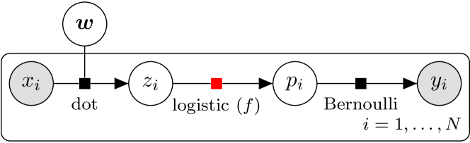
Figure 2: Factor graph for binary logistic regression. The kernel-based message operator learns to approximate the logistic factor highlighted in red. The two incoming messages are $m_{z_{i}\rightarrow f}=\mathcal{N}(z_{i};\mu,\sigma^{2})$ and $m_{p_{i}\rightarrow f}=\text{Beta}(p_{i};\alpha,\beta)$.

Experiment 1: Batch Learning

As in (Heess et al., 2013; Eslami et al., 2014), we study the logistic factor $f(p|z)=\delta\left(p-\frac{1}{1+\exp(-z)}\right),$ where $\delta$ is the Dirac delta function, in the context of a binary logistic regression model (Fig. 2). The factor is deterministic and there are two incoming messages: $m_{p_{i}\rightarrow f}=\text{Beta}(p_{i};\alpha,\beta)$ and $m_{z_{i}\rightarrow f}=\mathcal{N}(z_{i};\mu,\sigma^{2})$, where $z_{i}=\boldsymbol{w}^{\top}x_{i}$ represents the dot product between an observation $x_{i}\in\mathbb{R}^{d}$ and the coefficient vector $\boldsymbol{w}$ whose posterior is to be inferred.

In this first experiment we simply learn a kernel-based operator to send the message $m_{f\rightarrow z_{i}}$. Following Eslami et al. (2014), we set $d$ to 20, and generated 20 different datasets, sampling a different $\boldsymbol{w}\sim\mathcal{N}(0,I)$ and then a set of $\{(x_{i},y_{i})\}_{i=1}^{n}$ ($n=300$) observations according to the model. For each dataset we ran EP for 10 iterations, and collected incoming-outgoing message pairs in the first five iterations of EP from Infer.NET’s implementation of the logistic factor. We partitioned the messages randomly into 5,000 training and 3,000 test messages, and learned a message operator to predict $m_{f\rightarrow z_{i}}$ as described in Section 3. Regularization and kernel parameters were chosen by leave-one-out cross validation. We set the number of random features to $D_{in}=500$ and $D_{out}=1,000$; empirically, we observed no significant improvements beyond 1,000 random features.

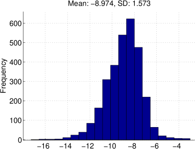
(a) KL errors

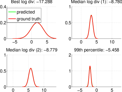
(b) Examples of predictions

Figure 3: Prediction errors for predicting the projected beliefs to $z_{i}$, and examples of predicted messages at different error levels.

We report $\log\mathrm{KL}[q_{f\rightarrow z_{i}}\|\hat{q}_{f\rightarrow z_{i}}]$ where $q_{f\rightarrow z_{i}}$ is the ground truth projected belief (numerator of (1)) and $\hat{q}_{f\rightarrow z_{i}}$ is the prediction. The histogram of the log KL errors is shown in Fig. 3a; Fig. 3b shows examples of predicted messages for different log KL errors. It is evident that the kernel-based operator does well in capturing the relationship between incoming and outgoing messages. The discrepancy with respect to the ground truth is barely visible even at the 99th percentile. See Section C in the supplementary material for a comparison with other methods.

Experiment 2: Uncertainty Estimates

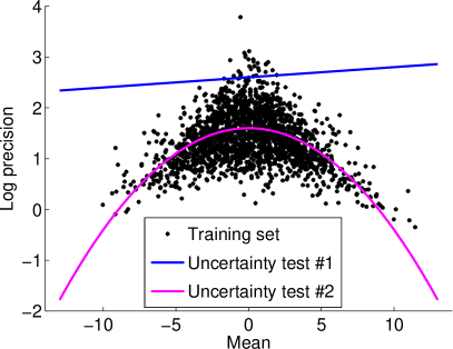
(a) Parameters of $m_{z_{i}\rightarrow f}$

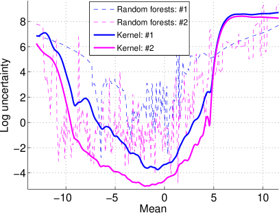
(b) Uncertainty estimates

Figure 4: (a) Incoming messages from $z$ to $f$ from 20 EP runs of binary logistic regression, as shown in Fig. 2. (b) Uncertainty estimates of the proposed kernel-based method (predictive variance) and Eslami et al.’s random forests (KL-based agreement of predictions of different trees) on the two uncertainty test sets shown. For testing, we fix the other incoming message $m_{p_{i}\rightarrow f}$ to $\text{Beta}(p_{i};1,2)$.

For the approximate message operator to perform well in a JIT learning setting, it is crucial to have reliable estimates of operator’s predictive uncertainty in different parts of the space of incoming messages. To assess this property we compute the predictive variance using the same learned operator as used in Fig. 3. The forward incoming messages $m_{z_{i}\rightarrow f}$ in the previously used training set are shown in Fig. 4a. The backward incoming messages $m_{p_{i}\rightarrow f}$ are not displayed. Shown in the same plot are two curves (a blue line, and a pink parabola) representing two “uncertainty test sets”: these are the sets of parameter pairs on which we wish to evaluate the uncertainty of the predictor, and pass through regions with both high and low densities of training samples. Fig. 4b shows uncertainty estimates of our kernel-based operator and of random forests, where we fix $m_{p_{i}\rightarrow f}:=\text{Beta}(p_{i};1,2)$ for testing. The implementation of the random forests closely follows Eslami et al. (2014).

From the figure, as the mean of the test message moves away from the region densely sampled by the training data, the predictive variance reported by the kernel method increases much more smoothly than that of the random forests. Further, our method clearly exhibits a higher uncertainty on the test set #1 than on the test set #2. This behaviour is desirable, as most of the points in test set #1 are either in a low density region or an unexplored region. These results suggest that the predictive variance is a robust criterion for querying the importance sampling oracle. One key observation is that the uncertainty estimates of the random forests are highly non-smooth; i.e., uncertainty on nearby points may vary wildly. As a result, a random forest-based JIT learner may still query the importance sampler oracle when presented with incoming messages similar to those in the training set, thereby wasting computation.

We have further checked that the predictive uncertainty of the regression function is a reliable indication of the error in KL divergence of the predicted outgoing messages. These results are given in Figure 10 of Appendix C.

Experiment 3: Just-In-Time Learning

In this experiment we test the approximate operator in the logistic regression model as part of the full EP inference loop in a just-in-time learning setting (KJIT). We now learn two kernel-based message operators, one for each outgoing direction from the logistic factor. The data generation is the same as in the batch learning experiment. We sequentially presented the operator with 30 related problems, where a new set of observations $\{(x_{i},y_{i})\}_{i=1}^{n}$ was generated at the beginning of each problem from the model, while keeping $\boldsymbol{w}$ fixed. This scenario is common in practice: one is often given several sets of observations which share the same model parameter (Eslami et al., 2014). As before, the inference target was $p(\boldsymbol{w}|\{(x_{i},y_{i})\}_{i=1}^{n})$. We set the maximum number of EP iterations to 10 in each problem.

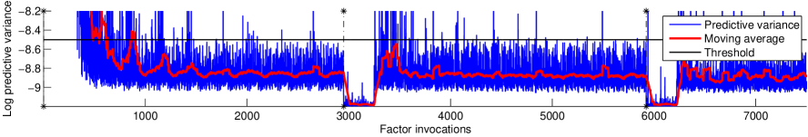
Figure 5: Uncertainty estimate of KJIT in its prediction of outgoing messages at each factor invocation, for the binary logistic regression problem. The black dashed lines indicate the start of a new inference problem.

We employed a “mini-batch” learning approach in which the operator always consults the oracle in the first few hundred factor invocations for initial batch training. In principle, during the initial batch training, the operator can perform cross validation or type-II maximum likelihood estimation for parameter selection; however for computational simplicity we set the kernel parameters according to the median heuristic (Schölkopf and Smola, 2002). Full detail of the heuristic is given in Section A in the supplementary material. The numbers of random features were $D_{\mathrm{in}}=300$ and $D_{\mathrm{out}}=500$. The output noise variance $\sigma^{2}_{y}$ was fixed to $10^{-4}$ and the uncertainty threshold on the log predictive variance was set to -8.5. To simulate a black-box setup, we used an importance sampler as the oracle rather than Infer.NET’s factor implementation, where the proposal distribution was fixed to $\mathcal{N}(z;0,200)$ with $5\times 10^{5}$ particles.

Fig. 5 shows a trace of the predictive variance of KJIT in predicting the mean of each $m_{f\rightarrow z_{i}}$ upon each factor invocation. The black dashed lines indicate the start of a new inference problem. Since the first 300 factor invocations are for the initial training, no uncertainty estimate is shown. From the trace, we observe that the uncertainty rapidly drops down to a stable point at roughly -8.8 and levels off after the operator sees about 1,000 incoming-outgoing message pairs, which is relatively low compared to approximately 3,000 message passings (i.e., 10 iterations $\times$ 300 observations) required for one problem. The uncertainty trace displays a periodic structure, repeating itself in every 300 factor invocations, corresponding to a full sweep over all 300 observations to collect incoming messages $m_{z_{i}\rightarrow f}$. The abrupt drop in uncertainty in the first EP iteration of each new problem is due to the fact that Infer.NET’s inference engine initializes the message from $\boldsymbol{w}$ to have zero mean, leading to $m_{z_{i}\rightarrow f}$ also having a zero mean. Repeated encounters of such a zero mean incoming message reinforce the operator’s confidence; hence the drop in uncertainty.

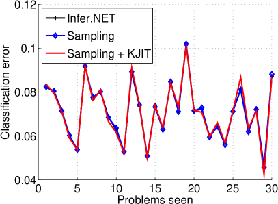
(a) Binary classification error

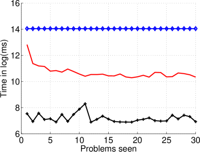
(b) Inference time

Figure 6: Classification performance and inference times of all methods in the binary logistic regression problem.

Fig. 6a shows binary classification errors obtained by using the inferred posterior mean of $\boldsymbol{w}$ on a test set of size 10000 generated from the true underlying parameter. Included in the plot are the errors obtained by using only the importance sampler for inference (“Sampling”), and using the Infer.NET’s hand-crafted logistic factor. The loss of KJIT matches well with that of the importance sampler and Infer.NET, suggesting that the inference accuracy is as good as these alternatives. Fig. 6b shows the inference time required by all methods in each problem. While the inference quality is equally good, KJIT is orders of magnitude faster than the importance sampler.

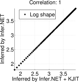
(a) Inferred shape

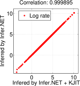
(b) Inferred rate

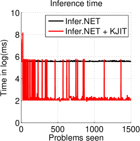
(c) Inference time

Figure 7: Shape (a) and rate (b) parameters of the inferred posteriors in the compound gamma problem. (c) KJIT is able to infer equally good posterior parameters compared to Infer.NET, while requiring a runtime several orders of magnitude lower.

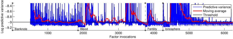
Figure 8: Uncertainty estimate of KJIT for outgoing messages on the four UCI datasets.

Experiment 4: Compound Gamma Factor

We next simulate the compound gamma factor, a heavy-tailed prior distribution on the precision of a Gaussian random variable. A variable $\tau$ is said to follow the compound gamma distribution if $\tau\sim\text{Gamma}(\tau;s_{2},r_{2})$ (shape-rate parameterization) and $r_{2}\sim\text{Gamma}(r_{2};s_{1},r_{1})$ where $(s_{1},r_{1},s_{2})$ are parameters. The task we consider is to infer the posterior of the precision $\tau$ of a normally distributed variable $x\sim\mathcal{N}(x;0,\tau)$ given realizations $\{x_{i}\}_{i=1}^{n}$. We consider the setting $(s_{1},r_{1},s_{2})=(1,1,1)$ which was used in Heess et al. (2013). Infer.NET’s implementation requires two gamma factors to specify the compound gamma. Here, we collapse them into one factor and let the operator learn to directly send an outgoing message $m_{f\rightarrow\tau}$ given $m_{\tau\rightarrow f}$, using Infer.NET as the oracle. The default implementation of Infer.NET relies on a quadrature method. As in Eslami et al. (2014), we sequentially presented a number of problems to our algorithm, where at the beginning of each problem, a random number of observations $n$ from 10 to 100, and the parameter $\tau$, were drawn from the model.

Fig. 7a and Fig. 7b summarize the inferred posterior parameters obtained from running only Infer.NET and Infer.NET + KJIT, i.e., KJIT with Infer.NET as the oracle. Fig. 7c shows the inference time of both methods. The plots collectively show that KJIT can deliver posteriors in good agreement with those obtained from Infer.NET, at a much lower cost. Note that in this task only one message is passed to the factor in each problem. Fig. 7c also indicates that KJIT requires fewer oracle consultations as more problems are seen.

Experiment 5: Classification Benchmarks

In the final experiment, we demonstrate that our method for learning the message operator is able to detect changes in the distribution of incoming messages via its uncertainty estimate, and to subsequently update its prediction through additional oracle queries. The different distributions of incoming messages are achieved by presenting a sequence of different classification problems to our learner. We used four binary classification datasets from the UCI repository (Lichman, 2013): banknote authentication, blood transfusion, fertility and ionosphere, in the same binary logistic regression setting as before. The operator was required to learn just-in-time to send outgoing messages $m_{f\rightarrow z_{i}}$ and $m_{f\rightarrow p_{i}}$ on the four problems presented in sequence. The training observations consisted of 200 data points subsampled from each dataset by stratified sampling. For the fertility dataset, which contains only 100 data points, we subsampled half the points. The remaining data were used as test sets. The uncertainty threshold was set to -9, and the minibatch size was 500. All other parameters were the same as in the earlier JIT learning experiment.

(a) Binary classification error

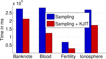
(b) Inference time

Figure 9: Classification performance and inference times on the four UCI datasets.

Classification errors on the test sets and inference times are shown in Fig. 9a and Fig. 9b, respectively. The results demonstrate that KJIT improves the inference time on all the problems without sacrificing inference accuracy. The predictive variance of each outgoing message is shown in Fig. 8. An essential feature to notice is the rapid increase of the uncertainty after the first EP iteration of each problem. As shown in Fig. 1, the distributions of incoming messages of the four problems are diverse. The sharp rise followed by a steady decrease of the uncertainty is a good indicator that the operator is able to promptly detect a change in input message distribution, and robustly adapt to this new distribution by querying the oracle.

5 CONCLUSIONS AND FUTURE WORK

We have proposed a method for learning the mapping between incoming and outgoing messages to a factor in expectation propagation, which can be used in place of computationally demanding Monte Carlo estimates of these updates. Our operator has two main advantages: it can reliably evaluate the uncertainty of its prediction, so that it only consults a more expensive oracle when it is uncertain, and it can efficiently update its mapping online, so that it learns from these additional consultations. Once trained, the learned mapping performs as well as the oracle mapping, but at a far lower computational cost. This is in large part due to a novel two-stage random feature representation of the input messages. One topic of current research is hyperparameter selection: at present, these are learned on an initial mini-batch of data, however a better option would be to adapt them online as more data are seen.

ACKNOWLEDGEMENT

We thank the anonymous reviewers for their constructive comments. WJ, AG, BL, and ZSz thank the Gatsby Charitable Foundation for the financial support.

Kernel-Based Just-In-Time Learning for Passing Expectation Propagation Messages

SUPPLEMENTARY MATERIAL

Appendix A MEDIAN HEURISTIC FOR GAUSSIAN KERNEL ON MEAN EMBEDDINGS

In the proposed KJIT, there are two kernels: the inner kernel $k$ for computing mean embeddings, and the outer Gaussian kernel $\kappa$ defined on the mean embeddings. Both of the kernels depend on a number of parameters. In this section, we describe a heuristic to choose the kernel parameters. We emphasize that this heuristic is merely for computational convenience. A full parameter selection procedure like cross validation or evidence maximization will likely yield a better set of parameters. We use this heuristic in the initial mini-batch phase before the actual online learning.

Let $\{r^{(l)}_{i}\mid l=1,\ldots,c,\text{ and }i=1,\ldots,n\}$ be a set of $n$ incoming message tuples collected during the mini-batch phase, from $c$ variables neighboring the factor. Let $R_{i}:=(r^{(l)}_{i})_{l=1}^{c}$ be the $i^{th}$ tuple, and let $\mathsf{r}_{i}:=\times_{l=1}^{c}r^{(l)}_{i}$ be the product of incoming messages in the $i^{th}$ tuple. Define $S_{i}$ and $\mathsf{s}_{i}$ to be the corresponding quantities of another tuple of messages. We will drop the subscript $i$ when considering only one tuple.

Recall that the kernel on two tuples of messages $R$ and $S$ is given by

$$\kappa(R,S) =\kappa(\mathsf{r},\mathsf{s})=\exp\left(-\frac{\|\mu_{\mathsf{r}}-\mu_{\mathsf{s}}\|_{\mathcal{H}}^{2}}{2\gamma^{2}}\right)$$

$$=\exp\left(-\frac{1}{2\gamma^{2}}\left\langle\mu_{\mathsf{r}},\mu_{\mathsf{r}}\right\rangle+\frac{1}{\gamma^{2}}\left\langle\mu_{\mathsf{r}},\mu_{\mathsf{s}}\right\rangle-\frac{1}{2\gamma^{2}}\left\langle\mu_{\mathsf{s}},\mu_{\mathsf{s}}\right\rangle\right),$$

where $\langle\mu_{\mathsf{r}},\mu_{\mathsf{s}}\rangle=\mathbb{E}_{x\sim\mathsf{r}}\mathbb{E}_{y\sim\mathsf{s}}k(x-y)$. The inner kernel $k$ is a Gaussian kernel defined on the domain $\mathcal{X}:=\mathcal{X}^{(1)}\times\cdots\times\mathcal{X}^{(c)}$ where $\mathcal{X}^{(l)}$ denotes the domain of $r^{(}l)$. For simplicity, we assume that $\mathcal{X}^{(l)}$ is one-dimensional. The Gaussian kernel $k$ takes the form

$$k(x-y) =\exp\left(-\frac{1}{2}\left(x-y\right)^{\top}\Sigma^{-1}\left(x-y\right)\right)=\prod_{l=1}^{c}\exp\left(-\frac{(x_{j}-y_{j})^{2}}{2\sigma^{2}_{l}}\right),$$

where $\Sigma=\mathop{\mathrm{diag}}(\sigma^{2}_{1},\ldots,\sigma^{2}_{c})$. The heuristic for choosing $\sigma^{2}_{1},\ldots,\sigma^{2}_{c}$ and $\gamma$ is as follows.

1. Set $\sigma_{l}^{2}:=\frac{1}{n}\sum_{i=1}^{n}\mathbb{V}_{x_{l}\sim r_{i}^{(l)}}[x_{l}]$ where $\mathbb{V}_{x_{l}\sim r_{i}^{(l)}}[x_{l}]$ denotes the variance of $r_{i}^{(l)}$.

2. With $\Sigma=\mathop{\mathrm{diag}}(\sigma^{2}_{1},\ldots,\sigma^{2}_{c})$ as defined in the previous step, set $\gamma^{2}:=\mathrm{median}\left(\{\|\mu_{\mathsf{r}_{i}}-\mu_{\mathsf{s}_{j}}\|^{2}\}_{i,j=1}^{n}\right)$.

Appendix B KERNELS AND RANDOM FEATURES

This section reviews relevant kernels and their random feature representations.

B.1 RANDOM FEATURES

This section contains a summary of Rahimi2007’s random Fourier features for a translation invariant kernel.

A kernel $k(x,y)=\left\langle\phi(x),\phi(y)\right\rangle$ in general may correspond to an inner product in an infinite-dimensional space whose feature map $\phi$ cannot be explicitly computed. In Rahimi2007, methods of computing an approximate feature maps $\hat{\phi}$ were proposed. The approximate feature maps are such that $k(x,y)\approx\hat{\phi}(x)^{\top}\hat{\phi}(y)$ (with equality in expectation) where $\hat{\phi}(x),\hat{\phi}(y)\in\mathbb{R}^{D}$ and $D$ is the number of random features. High $D$ yields a better approximation with higher computational cost. Assume $k(x,y)=k(x-y)$ (translation invariant) and $x,y\in\mathbb{R}^{d}$. Random Fourier features $\hat{\phi}(x)\in\mathbb{R}^{D}$ such that $k(x,y)\approx\hat{\phi}(x)^{\top}\hat{\phi}(y)$ are generated as follows:

1. Compute the Fourier transform $\hat{k}$ of the kernel $k$: $\hat{k}(\omega)=\frac{1}{2\pi}\int e^{-j\omega^{\top}\delta}k(\delta)\,d\delta$.

2. Draw $D$ i.i.d. samples $\omega_{1},\ldots,\omega_{D}\in\mathbb{R}^{d}$ from $\hat{k}$.

3. Draw $D$ i.i.d samples $b_{1},\ldots,b_{D}\in\mathbb{R}$ from $U[0,2\pi]$ (uniform distribution).

4. $\hat{\phi}(x)=\sqrt{\frac{2}{D}}\left(\cos\left(\omega_{1}^{\top}x+b_{1}\right),\ldots,\cos\left(\omega_{D}^{\top}x+b_{D}\right)\right)^{\top}\in\mathbb{R}^{D}$

Why It Works

Theorem 1.

Bochner’s theorem Rudin2013. A continuous kernel $k(x,y)=k(x-y)$ on $\mathbb{R}^{m}$ is positive definite iff $k(\delta)$ is the Fourier transform of a non-negative measure.

Furthermore, if a translation invariant kernel $k(\delta)$ is properly scaled, Bochner’s theorem guarantees that its Fourier transform $p(\omega)$ is a probability distribution. From this fact, we have

$$k(x-y)=\int\hat{k}(\omega)e^{j\omega^{\top}\left(x-y\right)}\,d\omega=\mathbb{E}_{\omega}\left[\eta_{\omega}(x)\eta_{\omega}(y)^{*}\right],$$

where $j=\sqrt{-1}$, $\eta_{\omega}(x)=e^{j\omega^{\top}x}$ and $\cdot^{*}$ denotes the complex conjugate. Since both $\hat{k}$ and $k$ are real, the complex exponential contains only the cosine terms. Drawing $D$ samples lowers the variance of the approximation.

Theorem 2.

Separation of variables. Let $\hat{f}$ be the Fourier transform of $f$. If $f(x_{1},\ldots,x_{d})=f_{1}(x_{1})\cdots f_{d}(x_{d})$, then $\hat{f}(\omega_{1},\ldots,\omega_{d})=\prod_{i=1}^{d}\hat{f}_{i}(\omega_{i})$.

Theorem 2 suggests that the random Fourier features can be extended to a product kernel by drawing $\omega$ independently for each kernel.

B.2 MV (MEAN-VARIANCE) KERNEL

Assume there are $c$ incoming messages $R:=\left(r^{(l)}\right)_{l=1}^{c}$ and $S:=\left(s^{(l)}\right)_{l=1}^{c}$ . Assume that

$$\mathbb{E}_{r^{(l)}}\left[x\right] =m_{l}$$

$$\mathbb{V}_{r^{(l)}}\left[x\right] =v_{l}$$

$$\mathbb{E}_{s^{(l)}}\left[y\right] =\mu_{l}$$

$$\mathbb{V}_{s^{(l)}}\left[y\right] =\sigma_{l}^{2}.$$

Incoming messages are not necessarily Gaussian. The MV (mean-variance) kernel is defined as a product kernel on means and variances.

$$\kappa_{\text{mv}}\left(R,S\right) =\prod_{i=1}^{c}k\left(\left(m_{i}-\mu_{i}\right)/w_{i}^{m}\right)\prod_{i=1}^{c}k\left(\left(v_{i}-\sigma_{i}^{2}\right)/w_{i}^{v}\right),$$

where $k$ is a Gaussian kernel with unit width. The kernel $\kappa_{\text{mv}}$ has $P:=\left(w_{1}^{m},\ldots,w_{c}^{m},w_{1}^{v},\ldots,w_{c}^{v}\right)$ as its parameters. With this kernel, we treat messages as finite dimensional vectors. All incoming messages $(s^{(i)})_{i=1}^{c}$ are represented as $\left(\mu_{1},\ldots,\mu_{c},\sigma_{1}^{2},\ldots,\sigma_{c}^{2}\right)^{\top}$. This treatment reduces the problem of having distributions as inputs to the familiar problem of having input points from a Euclidean space. The random features of Rahimi2007 can be applied straightforwardly.

B.3 EXPECTED PRODUCT KERNEL

Given two distributions $r(x)=\mathcal{N}(x;m_{r},V_{r})$ and $s(y)=\mathcal{N}(y;m_{s},V_{s})$ ($d$-dimensional Gaussian), the expected product kernel is defined as

$$\kappa_{\text{pro}}(r,s)=\left\langle\mu_{r},\mu_{s}\right\rangle_{\mathcal{H}}=\mathbb{E}_{r}\mathbb{E}_{s}k(x-y),$$

where $\mu_{r}:=\mathbb{E}_{r}k(x,\cdot)$ is the mean embedding of $r$, and we assume that the kernel $k$ associated with $\mathcal{H}$ is translation invariant i.e., $k(x,y)=k(x-y)$. The goal here is to derive random Fourier features for the expected product kernel. That is, we aim to find $\hat{\phi}$ such that $\kappa_{\text{pro}}(r,s)\approx\hat{\phi}(r)^{\top}\hat{\phi}(s)$ and $\hat{\phi}\in\mathbb{R}^{D}$.

We first give some results which will be used to derive the Fourier features for inner product of mean embeddings.

Lemma 3.

If $b\sim\mathcal{N}(b;0,\sigma^{2})$, then $\mathbb{E}[\cos(b)]=\exp\left(-\frac{1}{2}\sigma^{2}\right)$.

Proof.

We can see this by considering the characteristic function of $x\sim\mathcal{N}(x;\mu,\sigma^{2})$ which is given by

$$c_{x}(t)=\mathbb{E}_{x}\left[\exp\left(itb\right)\right]=\exp\left(itm-\frac{1}{2}\sigma^{2}t^{2}\right).$$

For $m=0,t=1$, we have

$$c_{b}(1)=\mathbb{E}_{b}\left[\exp(ib)\right]=\exp\left(-\frac{1}{2}\sigma^{2}\right)=\mathbb{E}_{b}\left[\cos(b)\right],$$

where the imaginary part $i\sin(tb)$ vanishes. ∎

From Rahimi2007 which provides random features for $k(x-y)$, we immediately have

$$\mathbb{E}_{r}\mathbb{E}_{s}k(x-y) \approx\mathbb{E}_{r}\mathbb{E}_{s}\frac{2}{D}\sum_{i=1}^{D}\cos\left(w_{i}^{\top}x+b_{i}\right)\cos\left(w_{i}^{\top}y+b_{i}\right)$$

$$=\frac{2}{D}\sum_{i=1}^{D}\mathbb{E}_{r(x)}\cos\left(w_{i}^{\top}x+b_{i}\right)\mathbb{E}_{s(y)}\cos\left(w_{i}^{\top}y+b_{i}\right),$$

where $\{w_{i}\}_{i=1}^{D}\sim\hat{k}(w)$ (Fourier transform of $k$) and $\{b_{i}\}_{i=1}^{D}\sim U\left[0,2\pi\right]$.

Consider $\mathbb{E}_{r(x)}\cos\left(w_{i}^{\top}x+b_{i}\right)$. Define $z_{i}=w_{i}^{\top}x+b_{i}$. So $z_{i}\sim\mathcal{N}(z_{i};w_{i}^{\top}m_{r}+b_{i},w_{i}^{\top}V_{r}w_{i})$. Let $d_{i}\sim\mathcal{N}(0,w_{i}^{\top}V_{r}w_{i})$. Then, $r(d_{i}+w_{i}^{\top}m_{r}+b_{i})=\mathcal{N}(w_{i}^{\top}m_{r}+b_{i},w_{i}^{\top}V_{r}w_{i})$ which is the same distribution as that of $z_{i}$. From these definitions we have,

$$\mathbb{E}_{r(x)}\cos\left(w_{i}^{\top}x+b_{i}\right) =\mathbb{E}_{r(z_{i})}\cos(z_{i})$$

$$=\mathbb{E}_{r(d_{i})}\cos\left(d_{i}+w_{i}^{\top}m_{r}+b_{i}\right)$$

$$\overset{(a)}{=}\mathbb{E}_{r(d_{i})}\cos(d_{i})\cos(w_{i}^{\top}m_{r}+b_{i})-\mathbb{E}_{r(d_{i})}\sin(d_{i})\sin(w_{i}^{\top}m_{r}+b_{i})$$

$$\overset{(b)}{=}\cos(w_{i}^{\top}m_{r}+b_{i})\mathbb{E}_{r(d_{i})}\cos(d_{i})$$

$$\overset{(c)}{=}\cos(w_{i}^{\top}m_{r}+b_{i})\exp\left(-\frac{1}{2}w_{i}^{\top}V_{r}w_{i}\right),$$

where at $(a)$ we use $\cos(\alpha+\beta)=\cos(\alpha)\cos(\beta)-\sin(\alpha)\sin(\beta)$. We have $(b)$ because $\sin$ is an odd function and $\mathbb{E}_{r(d_{i})}\sin(d_{i})=0$. The last equality $(c)$ follows from Lemma 3. It follows that the random features $\hat{\phi}(r)\in\mathbb{R}^{D}$ are given by

$$\hat{\phi}(r)=\sqrt{\frac{2}{D}}\left(\begin{array}[]{c}\cos(w_{1}^{\top}m_{r}+b_{1})\exp\left(-\frac{1}{2}w_{1}^{\top}V_{r}w_{1}\right)\\ \vdots\\ \cos(w_{D}^{\top}m_{r}+b_{D})\exp\left(-\frac{1}{2}w_{D}^{\top}V_{r}w_{D}\right)\end{array}\right).$$

Notice that the translation invariant kernel $k$ provides $\hat{k}$ from which $\{w_{i}\}_{i}$ are drawn. For a different type of distribution $r$, we only need to be able to compute $\mathbb{E}_{r(x)}\cos\left(w_{i}^{\top}x+b_{i}\right)$. With $\hat{\phi}(r)$, we have $\kappa_{\text{pro}}(r,s)\approx\hat{\phi}(r)^{\top}\hat{\phi}(s)$ with equality in expectation.

Analytic Expression for Gaussian Case

For reference, if $r,s$ are normal distributions and $k$ is a Gaussian kernel, an analytic expression is available. Assume $k(x-y)=\exp\left(-\frac{1}{2}\left(x-y\right)^{\top}\Sigma^{-1}\left(x-y\right)\right)$ where $\Sigma$ is the kernel parameter. Then

$$\mathbb{E}_{r}\mathbb{E}_{s}k(x-y) =\sqrt{\frac{\det(D_{rs})}{\det(\Sigma^{-1})}}\exp\left(-\frac{1}{2}\left(m_{r}-m_{s}\right)^{\top}D_{rs}\left(m_{r}-m_{s}\right)\right),$$

$$D_{rs} :=\left(V_{r}+V_{s}+\Sigma\right)^{-1}.$$

Approximation Quality

The following result compares the randomly generated features to the true kernel matrix using various numbers of random features $D$. For each $D$, we repeat 10 trials, where the randomness in each trial arises from the construction of the random features. Samples are univariate normal distributions $\mathcal{N}(m,v)$ where $m\sim\mathcal{N}(0,9)$ and $v\sim\text{Gamma}(3,1/4)$ (shape-rate parameterization). The kernel parameter was $\Sigma:=\sigma^{2}I$ where $\sigma^{2}=3$.

“max entry diff” refers to the maximum entry-wise difference between the true kernel matrix and the approximated kernel matrix.

B.4 PRODUCT KERNEL ON MEAN EMBEDDINGS

Previously, we have defined an expected product kernel on single distributions. One way to define a kernel between two tuples of more than one incoming message is to take a product of the kernels defined on each message.

Let $\mu_{r^{(l)}}:=\mathbb{E}_{r^{(l)}(a)}k^{(l)}(\cdot,a)$ be the mean embedding Smola2007 of the distribution $r^{(l)}$ into RKHS $\mathcal{H}^{(l)}$ induced by the kernel $k$. Assume $k^{(l)}=k_{\text{gauss}}^{(l)}$ (Gaussian kernel) and assume there are $c$ incoming messages $R:=(r^{(i)}(a^{(i)}))_{i=1}^{c}$ and $S:=(s^{(i)}(b^{(i)}))_{i=1}^{c}$. A product of expected product kernels is defined as

$$\kappa_{\text{pro, prod}}(R,S) :=\left\langle\bigotimes_{l=1}^{c}\mu_{r^{(l)}},\bigotimes_{l=1}^{c}\mu_{s^{(l)}}\right\rangle_{\otimes_{l}\mathcal{H}^{(l)}}$$

$$=\prod_{l=1}^{c}\mathbb{E}_{r^{(l)}(a^{(l)})}\mathbb{E}_{s^{(l)}(b^{(l)})}k_{\text{gauss}}^{(l)}\left(a^{(l)},b^{(l)}\right)\approx\hat{\phi}(R)^{\top}\hat{\phi}(S),$$

where $\hat{\phi}(R)^{\top}\hat{\phi}(S)=\prod_{l=1}^{c}\hat{\phi}^{(l)}(r^{(l)})^{\top}\hat{\phi}^{(l)}(s^{(l)})$. The feature map $\hat{\phi}^{(l)}(r^{(l)})$ can be estimated by applying the random Fourier features to $k_{\text{gauss }}^{(l)}$and taking the expectations $\mathbb{E}_{r^{(l)}(a)}\mathbb{E}_{s^{(l)}(b)}$. The final feature map is $\hat{\phi}(R)=\hat{\phi}^{(1)}(r^{(1)})\circledast\hat{\phi}^{(2)}(r^{(2)})\circledast\cdots\circledast\hat{\phi}^{(c)}(r^{(c)})\in\mathbb{R}^{D^{c}}$, where $\circledast$ denotes a Kronecker product and we assume that $\hat{\phi}^{(l)}\in\mathbb{R}^{D}$ for $l\in\{1,\ldots,c\}$.

B.5 SUM KERNEL ON MEAN EMBEDDINGS

If we instead define the kernel as the sum of $c$ kernels, we have

$$\kappa_{\text{pro, sum}}(R,S) =\sum_{l=1}^{c}\left\langle\mu_{r^{(l)}},\mu_{s^{(l)}}\right\rangle_{\mathcal{H}^{(l)}}$$

$$\approx\sum_{l=1}^{c}\hat{\phi}^{(l)}(r^{(l)})^{\top}\hat{\phi}^{(l)}(s^{(l)})$$

$$=\hat{\varphi}(R)^{\top}\hat{\varphi}(S),$$

where $\hat{\varphi}(R):=\left(\hat{\phi}^{(1)}(r^{(1)})^{\top},\ldots,\hat{\phi}^{(c)}(r^{(c)})^{\top}\right)^{\top}\in\mathbb{R}^{cD}$.

B.6 NUMBER OF RANDOM FEATURES FOR GAUSSIAN KERNEL ON MEAN EMBEDDINGS

We quantify the effect of $D_{\mathrm{in}}$ and $D_{\mathrm{out}}$ empirically as follows. We generate 300 Gaussian messages, compute the true Gram matrix and the approximate Gram matrix given by the random features, and report the Frobenius norm of the difference of the two matrices on a grid of $D_{\mathrm{in}}$ and $D_{\mathrm{out}}$. For each $(D_{\mathrm{in}},D_{\mathrm{out}})$, we repeat 20 times with a different set of random features and report the averaged Frobenius norm.

The result suggests that $D_{\mathrm{out}}$ has more effect in improving the approximation.

Appendix C MORE DETAILS ON EXPERIMENT 1: BATCH LEARNING

There are a number of kernels on distributions we may use for just-in-time learning. To find the most suitable kernel, we compare the performance of each on a collection of incoming and output messages at the logistic factor in the binary logistic regression problem i.e., same problem as in experiment $1$ in the main text. All messages are collected by running EP 20 times on generated toy data. Only messages in the first five iterations are considered as messages passed in the early phase of EP vary more than in a near-convergence phase. The regression output to be learned is the numerator of (1).

A training set of 5000 messages and a test set of 3000 messages are obtained by subsampling all the collected messages. Where random features are used, kernel widths and regularization parameters are chosen by leave-one-out cross validation. To get a good sense of the approximation error from the random features, we also compare with incomplete Cholesky factorization (denoted by IChol), a widely used Gram matrix approximation technique. We use hold-out cross validation with randomly chosen training and validation sets for parameter selection, and kernel ridge regression in its dual form when the incomplete Cholesky factorization is used.

Let $f$ be the logistic factor and $m_{f\rightarrow i}$ be an outgoing message. Let $q_{f\rightarrow i}$ be the ground truth belief message (numerator) associated with $m_{f\rightarrow i}$. The error metric we use is $\mathrm{KL}[q_{f\rightarrow i}\,||\,\hat{q}_{f\rightarrow i}]$ where $\hat{q}_{f\rightarrow i}$ are the belief messages estimated by a learned regression function. The following table reports the mean of the log KL-divergence and standard deviations.

	mean log KL	s.d. of log KL
Random features + MV Kernel	-6.96	1.67
Random features + Expected product kernel on joint embeddings	-2.78	1.82
Random features + Sum of expected product kernels	-1.05	1.93
Random features + Product of expected product kernels	-2.64	1.65
Random features + Gaussian kernel on joint embeddings (KJIT)	-8.97	1.57
IChol + sum of Gaussian kernel on embeddings	-2.75	2.84
IChol + Gaussian kernel on joint embeddings	-8.71	1.69
Breiman’s random forests Breiman2001	-8.69	1.79
Extremely randomized trees Geurts2006	-8.90	1.59
Eslami2014’s random forests Eslami2014	-6.94	3.88

The MV kernel is defined in Section B.2. Here product (sum) of expected product kernels refers to a product (sum) of kernels, where each is an expected product kernel defined on one incoming message. Evidently, the Gaussian kernel on joint mean embeddings performs significantly better than other kernels. Besides the proposed method, we also compare the message prediction performance to Breiman’s random forests Breiman2001, extremely randomized trees Geurts2006, and Eslami2014’s random forests. We use scikit-learn toolbox for the extremely randomized trees and Breiman’s random forests. For Eslami2014’s random forests, we reimplemented the method as closely as possible according to the description given in Eslami2014. In all cases, the number of trees is set to 64. Empirically we observe that decreasing the log KL error below -8 will not yield a noticeable performance gain in the actual EP.

To verify that the uncertainty estimates given by KJIT coincide with the actual predictive performance (i.e., accurate prediction when confident), we plot the predictive variance against the KL-divergence error on both the training and test sets. The results are shown in Fig. 10. The uncertainty estimates show a positive correlation with the KL-divergence errors. It is instructive to note that no point lies at the bottom right i.e., making a large error while being confident. The fact that the errors on the training set are roughly the same as the errors on the test set indicates that the operator does not overfit.

Figure 10: KL-divergence error versus predictive variance for predicting the mean of $m_{f\rightarrow z_{i}}$ (normal distribution) in the logistic factor problem.

abbrvnat refappendix

References

- Alvarez et al. (2011) M. A. Alvarez, L. Rosasco, and N. D. Lawrence. Kernels for vector-valued functions: a review. 2011. URL http://arxiv.org/abs/1106.6251.