Fitting 3D Morphable Models using Local Features
Abstract
In this paper, we propose a novel fitting method that uses local image features to fit a 3D Morphable Model to 2D images. To overcome the obstacle of optimising a cost function that contains a non-differentiable feature extraction operator, we use a learning-based cascaded regression method that learns the gradient direction from data. The method allows to simultaneously solve for shape and pose parameters. Our method is thoroughly evaluated on Morphable Model generated data and first results on real data are presented. Compared to traditional fitting methods, which use simple raw features like pixel colour or edge maps, local features have been shown to be much more robust against variations in imaging conditions. Our approach is unique in that we are the first to use local features to fit a Morphable Model.
Because of the speed of our method, it is applicable for real-time applications. Our cascaded regression framework is available as an open source library111https://github.com/patrikhuber.
Index Terms:
3D Morphable Model, cascaded regression, local features, SIFT, 3D reconstruction, supervised descent.I Introduction
This work tackles the problem of obtaining a 3D representation of a face from a single 2D image, which is an inherently ill-posed problem with many free parameters: the orientation of the face, identity and lighting, amongst others. A 3D Morphable Face Model (3DMM) [1, 2] usually consists of a PCA model of shape and one of color (albedo), camera and a lighting model. To fit the model to a 2D image, or in other words, to reconstruct all these model parameters, a cost function is set up and optimised.
Existing so-called fitting algorithms that define and solve these cost functions can loosely be classified into two categories: the ones with linear cost functions and those with non-linear cost functions. Algorithms that fall into the first category typically use only facial landmarks like eye or mouth corners to fit shape and camera parameters, and use image information (pixel values) to fit an albedo and light model [3, 4]. Often, these steps are separate and applied iteratively. The second class of algorithms traditionally consists of a more complex cost function, using the image information to perform shape from shading, edge detection, and applying a nonlinear solver to jointly or iteratively solve for all the parameters [5, 6, 7, 8]. Recently, Schönborn et al. proposed a Markov Chain Monte Carlo based fitting method that integrates automatic landmark detections [9, 10]. Most of these algorithms require several minutes to fit a single image.
A common point of these algorithms is that they use either only landmark information or simple features like raw color values or edge maps, while in a lot of other domains, most notably 2D facial landmark detection, these have long been superseded by local image features like Histogram of Oriented Gradient (HoG) [11] or Scale Invariant Feature Transform (SIFT) [12]. However, it is non-trivial to use such features to fit 3D Morphable Models: they are non-differentiable operators and have not yet been used for 3DMM fitting.
Recently, cascaded-regression based methods have been widely used with promising results in pose estimation [13, 14] and 2D face alignment [15, 16, 17, 18]. In general, a discriminative cascaded regression based method performs optimisation in local feature space by applying a learning-based approach to circumvent the problem of non-differentiability. The method allows to learn the gradient of a function from data, instead of differentiating. In this paper, we propose to use a similar strategy to perform 3DMM fitting using SIFT features.
In comparison with existing 3DMM fitting algorithms, using image features and a cascaded regression based approach has the potential to give the best of the two worlds: it is fast, like the linear landmarks-only fitting methods, and at the same time robust to changing image conditions, and it can be potentially more precise, because image information is used to fit shape and pose, and not only landmarks. Furthermore, it is possible to solve for pose and shape parameters simultaneously, instead of iteratively. This paper introduces and evaluates the proposed novelty in the context of fitting pose and shape parameters.
In the rest of this paper, we first give a brief introduction to the cascaded regression method and 3DMMs (Section II). In Section III, we present the concept of using local image features to fit a 3D Morphable Model, and show how cascaded regression is applied to optimise the Morphable Model parameters in local feature space. We thoroughly evaluate our method using pose and shape data generated from the Morphable Model, as well as on PIE fitting results (Section IV). Section V concludes the paper.
II Background
Given an input face image and a pre-trained 3DMM, our goal is to find the pose and shape parameters of the 3DMM that best represent the face. In our setting, a face box or facial landmarks are given to perform a rough initialisation of the model. The goal is then to obtain an accurate fitting result using a cost function that incorporates the image information in the form of local features. To facilitate this, the cascaded regression framework is used to learn a series of regressors.
In this section, we will briefly introduce the generic cascaded regression framework and the 3D Morphable Model. The 3D Morphable Model fitting using local image features will then be introduced in Section III.
II-A Cascaded Regression
Given an input image and a pre-trained model with respect to a parameter vector , the aim of a regression based method is to iteratively update the parameters to maximise the posterior probability . A regression based method solves this non-linear optimisation problem by learning the gradient from a set of training samples in a supervised manner. The goal is to find a regressor:
| (1) |
where is a vector of extracted features from the input image, given the current model parameters, and is the predicted model parameter update. This mapping can be learned from a training dataset using any regression method, e.g. linear regression [15, 18], random forests [16] or artificial neural networks [17]. In contrast to these regression algorithms, a cascaded regression method generates a strong regressor consisting of weak regressors in cascade:
| (2) |
where is the th weak regressor in cascade. In this paper, we use a simple linear regressor:
| (3) |
where is the projection matrix and is the offset (bias) of the th weak regressor.
More specifically, given a set of training samples , we first apply the ridge regression algorithm to learn the first weak regressor by minimising the loss:
| (4) |
and then update the training samples, i.e. the model parameters and the corresponding feature vectors, using the learned regressor to generate a new training dataset for the second weak regressor learning. This process is repeated until convergence or exceeding a pre-defined maximum number of regressors.
In the test phase, these pre-trained weak regressors are progressively applied to an input image with an initial model parameter estimate to update the model and output the final fitting result.
II-B The 3D Morphable Model
A 3D Morphable Model consists of a shape and albedo (color) PCA model, of which we use the shape model in this paper. It is constructed from 3D face meshes that are in dense correspondence, that is, vertices with the same index in the mesh correspond to the same semantic point on each face. In 3DMM, a 3D shape is expressed as , where are the coordinates of the th vertex and is the number of mesh vertices. PCA is then applied to this data matrix consisting of stacked 3D face meshes, which yields eigenvectors , their corresponding variances , and a mean shape . A face can then be approximated as a linear combination of the basis vectors:
| (5) |
where is the shape coefficient or parameter vector.
III 3D Morphable Model Fitting using Local Image Features
In this section, we will present how we formulate the cascaded regression approach to perform model-fitting using local features.
III-A Local Feature based Pose Fitting
To estimate the pose of the 3D model, we select the parameters vector to be , with , , and being the pitch, yaw and roll angle respectively, and , and the translations in 3D model space. We can then project a point in homogeneous coordinates from 3D space to 2D using a standard perspective projection:
| (6) |
where , and are rotation, translation and projection matrices respectively, constructed from the values in , followed by perspective division and converting to screen coordinates.
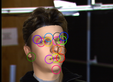
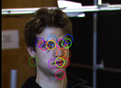
From the full 3D model’s mesh, we choose a subset of 3D vertices from the mean shape model in homogeneous coordinates, i.e. , . Given the current pose parameters we then project them onto the 2D image to obtain a set of 2D coordinates . Next, local features are extracted from the image around these projected 2D locations, resulting in feature vectors , where , in our case of SIFT features. These feature vectors are then concatenated to form one final feature vector, which is the output of and the input for the regressor. Figure 1 shows an overview of the process with an input image, the projected 3D model, the locations used to extract local features and their respective location in the input image.

III-B Local Feature based Shape Fitting
As the cascaded regression method allows to estimate arbitrary parameters, we can apply it to estimating the shape parameters in local feature space as well. Our motivation is that the image data contains information about a face’s shape, and we want to reconstruct the model’s shape parameters for the subject in a given image. Similar to the previous section, we select a number of 3D vertices , but instead of using the mean mesh, we generate a face instance using the current estimated shape coefficients and then use these identity-specific vertex coordinates to project to 2D space.
More specifically, we construct a matrix by selecting the rows of the PCA basis matrix corresponding to the chosen vertex points. A face shape is generated with the formula in equation 5, using and the current estimate of . The parameter vector is then extended to incorporate the shape coefficients: .
Given a new image with a face, and initial landmark locations, initial values for the pose parameter part of are calculated. The shape initialisation is started at the mean face (). The model is projected using this initial estimate, and local features are extracted at the projected 2D locations. Using these features, the regressor predicts a parameter update , and the process is repeated using the new parameter estimate.
While in our case, the points on the mesh we selected coincide with distinctive facial feature points like the eye or mouth corners, any vertex from the 3D model can be used, for example, the points could be spaced equidistant on the 3D face mesh.
It is noteworthy that our method does not rely on particular detected 2D landmarks. A rough initialisation is sufficient to run the cascaded regression. In essence, the proposed method can also be seen as a 3D model based landmark detection, steering the 3D model parameters to converge to the ground truth location. This presents a novel step towards unifying landmark detection and 3D Morphable Model fitting.
IV Experimental Results
In the following, we present results of the learning based cascaded regression method for pose fitting. Accurate ground truth is obtained by generating synthetic data using the 3D Morphable Model. To simulate more realistic conditions, for each image, a random background is chosen from a backgrounds dataset.
In a second experiment, we perform simultaneous shape and pose fitting using the same method. We subsequently compare the proposed method with POSIT [19] and present results on the PIE database.
IV-A Pose Fitting
In this first experiment, we evaluate our method by estimating the 3D pose from the extracted local image features. To train the cascaded regression, we generate poses from to yaw and pitch variation, in intervals. Additionally, Gaussian noise with mm in x and y translation is added to simulate imprecise initialisation. The model is placed at an initial z-location of mm and the focal length was fixed to . Each sample generated in this way is duplicated and used with 5 different backgrounds. Parameter initialisations are generated by perturbing every angle of each sample with a value uniformly drawn from the interval .
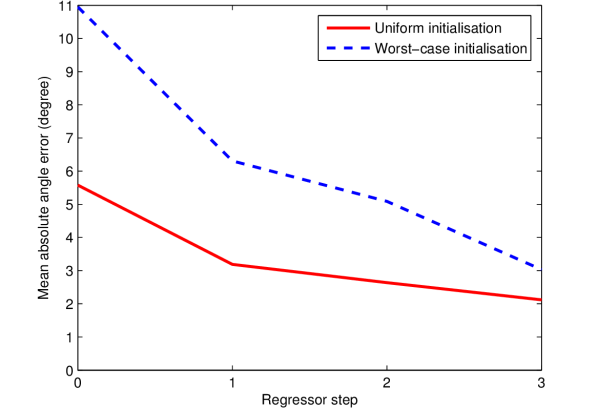
The cascaded regression is tested on the same angle range, but we sample the test data at a finer resolution of intervals to verify correct approximation of the learned function. Figure 2 shows the mean absolute error of all three predicted angles on the test data. The optimisation is initialised in two different ways: first, with values uniformly drawn in the interval around the ground truth, and second, to evaluate the performance in the case of bad initialisation, the samples are placed away from the ground truth in all the images. In both cases, the algorithm converges, and each regressor step promotes further convergence.
IV-B Simultaneous Shape- and Pose Fitting
The cascaded regression method allows us to simultaneously estimate the shape parameters together with the pose parameters in a unified way. The parameter vector is extended to include the first two PCA shape coefficients of the Morphable Model: . We generate test data following the same protocol as described in Section IV-A, with the addition that the identity of each test sample is learned as well.
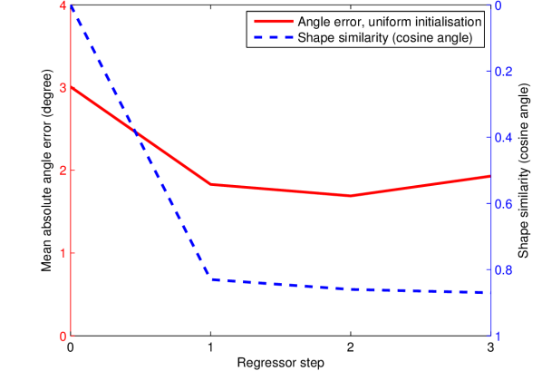
Figure 3 shows the results of the joint shape- and pose fitting. The shape fitting accuracy is measured by the cosine angle between the coefficients of the ground truth and the estimated face : . A shape similarity of 0.87 is achieved, and the pose estimation slightly improves compared to the previous experiment, because the pose can be more accurately estimated when the shape is allowed to change. Similar to the first experiment, this experimental study shows promising results for the local feature based fitting method.
IV-C Comparison against POSIT
To relate the performance of our method to existing solutions in the literature, we compare the pose-fitting part of our algorithm against POSIT (Pose from Orthography and Scaling with ITerations). POSIT estimates the pose from a set of 2D to 3D correspondences. In our case, the 2D points are the ground truth landmarks. Tested on the same data as in Section IV-A, POSIT achieves a mean absolute error over all angles of , compared to around for our method. It should be noted that POSIT achieves these results with very accurate ground truth landmarks, which are often not available in practical applications. If Gaussian noise of 5 pixels is added to the landmarks, the accuracy of POSIT drops to . In contrast to that, the proposed algorithm does not rely on detected landmarks and their accuracy.
IV-D Evaluation on PIE
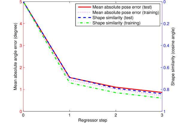
To evaluate the proposed method on real data, we use the fitting results on the PIE database [20] that are provided with the Basel Face Model (BFM, [21]) as ground truth data. In this way, we can evaluate how well the proposed method can approximate a complex state of the art fitting method. In particular, to evaluate how the proposed method is able to estimate the shape and pose under changing illumination conditions, we split the available PIE data into illuminations 1 to 17 for training and 18 to 22 for testing, resulting in 3468 training and 1020 test images. Again, a 3-stage cascaded regressor is learned.
Figure 4 shows the mean absolute angle error on the training and test set, as well as the cosine angle of the shape coefficients. It can be seen that the test error is only marginally higher than the training error, and the proposed method generalises well to unseen illumination conditions. On the test data, the angle is estimated with an average error of , and a shape similarity of 0.84 is achieved.
IV-E Runtime
Cascaded regression methods are inherently fast, and so is the proposed local feature based Morphable Model fitting. Estimating the pose and shape requires around 200 milliseconds per image, with an unoptimised implementation. The runtime largely depends on the number of vertices that are used for local feature extraction, as they directly influence the dimensionality of the feature vector (and thus the prediction time of the regressor). The algorithm could further be sped up by using faster feature extraction or compressing the feature vectors using PCA, but it has, already in its current form, the potential to be used in real-time applications and in a large-scale fashion.
V Conclusion
We proposed a new way to fit 3D Morphable Models that uses local image features. We overcome the obstacle of solving a cost function that contains a non-differentiable feature extraction operator by using a learning-based cascaded regression method that learns the gradient direction from data. We evaluated the proposed method on accurate Morphable Model generated data as well as on real images. The method yields promising results, as local features have been proven robust in many vision algorithms. In contrast to many existing fitting algorithms, our algorithm achieves near real-time performance. Future work includes further evaluation of how the proposed method can unify landmark detection and 3D Morphable Model fitting, and fitting of more shape and possibly albedo coefficients.
References
- [1] V. Blanz and T. Vetter, “A morphable model for the synthesis of 3d faces,” in Proceedings of the 26th annual conference on Computer graphics and interactive techniques. ACM Press/Addison-Wesley Publishing Co., 1999, pp. 187–194.
- [2] ——, “Face recognition based on fitting a 3d morphable model,” Pattern Analysis and Machine Intelligence, IEEE Transactions on, vol. 25, no. 9, pp. 1063–1074, 2003.
- [3] O. Aldrian and W. A. Smith, “Inverse rendering of faces with a 3d morphable model,” Pattern Analysis and Machine Intelligence, IEEE Transactions on, vol. 35, no. 5, pp. 1080–1093, 2013.
- [4] S. Romdhani, V. Blanz, and T. Vetter, “Face identification by fitting a 3d morphable model using linear shape and texture error functions,” in European Conference on Computer Vision, 2002, pp. 3–19.
- [5] S. Romdhani and T. Vetter, “Estimating 3d shape and texture using pixel intensity, edges, specular highlights, texture constraints and a prior,” in Computer Vision and Pattern Recognition., vol. 2. IEEE, 2005, pp. 986–993.
- [6] R. T. A. van Rootseler, L. J. Spreeuwers, and R. N. J. Veldhuis, “Using 3d morphable models for face recognition in video,” in Proceedings of the 33rd WIC Symposium on Information Theory in the Benelux, 2012.
- [7] J. Tena, R. Smith, M. Hamouz, J. Kittler, A. Hilton, and J. Illingworth, “2d face pose normalisation using a 3d morphable model,” in IEEE Conference on Advanced Video and Signal Based Surveillance (AVSS), Sep. 2007, pp. 51 –56.
- [8] G. Hu, C.-H. Chan, J. Kittler, and B. Christmas, “Resolution-aware 3d morphable model,” in BMVC, 2012, pp. 1–10.
- [9] S. Schönborn, A. Forster, B. Egger, and T. Vetter, “A monte carlo strategy to integrate detection and model-based face analysis,” in Proceedings of the 35th German Conference on Pattern Recognition, vol. 8142. Springer Berlin Heidelberg, Sep. 2013, pp. 101–110.
- [10] B. Egger, S. Schönborn, A. Forster, and T. Vetter, “Pose normalization for eye gaze estimation and facial attribute description from still images,” in 36th German Conference on Pattern Recognition, Sep. 2014.
- [11] N. Dalal and B. Triggs, “Histograms of oriented gradients for human detection,” in Computer Vision and Pattern Recognition (CVPR), IEEE Computer Society Conference on, vol. 1, 2005, pp. 886–893.
- [12] D. G. Lowe, “Distinctive image features from scale-invariant keypoints,” International journal of computer vision, vol. 60, no. 2, pp. 91–110, 2004.
- [13] P. Dollár, P. Welinder, and P. Perona, “Cascaded pose regression,” in IEEE Conference on Computer Vision and Pattern Recognition (CVPR), 2010, pp. 1078–1085.
- [14] M. Rätsch, P. Quick, P. Huber, T. Frank, and T. Vetter, “Wavelet reduced support vector regression for efficient and robust head pose estimation,” in Ninth Conference on Computer and Robot Vision (CRV), May 2012, pp. 260–267.
- [15] X. Xiong and F. De la Torre, “Supervised descent method and its applications to face alignment,” in Computer Vision and Pattern Recognition (CVPR), IEEE Conference on, 2013, pp. 532–539.
- [16] X. Cao, Y. Wei, F. Wen, and J. Sun, “Face alignment by explicit shape regression,” International Journal of Computer Vision, vol. 107, no. 2, pp. 177–190, 2014.
- [17] Y. Sun, X. Wang, and X. Tang, “Deep convolutional network cascade for facial point detection,” in Computer Vision and Pattern Recognition (CVPR), IEEE Conference on, 2013, pp. 3476–3483.
- [18] Z.-H. Feng, P. Huber, J. Kittler, W. Christmas, and X.-J. Wu, “Random cascaded-regression copse for robust facial landmark detection,” Signal Processing Letters, IEEE, vol. 22, no. 1, pp. 76–80, Jan 2015.
- [19] D. F. Dementhon and L. S. Davis, “Model-based object pose in 25 lines of code,” International Journal of Computer Vision, vol. 15, no. 1-2, pp. 123–141, Jun. 1995.
- [20] T. Sim, S. Baker, and M. Bsat, “The CMU pose, illumination, and expression database,” IEEE Transactions on Pattern Analysis and Machine Intelligence, vol. 25, pp. 1615–1618, 2003.
- [21] P. Paysan, R. Knothe, B. Amberg, S. Romdhani, and T. Vetter, “A 3d face model for pose and illumination invariant face recognition,” in Proceedings of the 6th IEEE International Conference on Advanced Video and Signal based Surveillance (AVSS), Genova, Italy, 2009.