Learning to rank in person re-identification with metric ensembles

Abstract

We propose an effective structured learning based approach to the problem of person re-identification which outperforms the current state-of-the-art on most benchmark data sets evaluated. Our framework is built on the basis of multiple low-level hand-crafted and high-level visual features. We then formulate two optimization algorithms, which directly optimize evaluation measures commonly used in person re-identification, also known as the Cumulative Matching Characteristic (CMC) curve. Our new approach is practical to many real-world surveillance applications as the re-identification performance can be concentrated in the range of most practical importance. The combination of these factors leads to a person re-identification system which outperforms most existing algorithms. More importantly, we advance state-of-the-art results on person re-identification by improving the rank-$1$ recognition rates from $40\%$ to $50\%$ on the iLIDS benchmark, $16\%$ to $18\%$ on the PRID2011 benchmark, $43\%$ to $46\%$ on the VIPeR benchmark, $34\%$ to $53\%$ on the CUHK01 benchmark and $21\%$ to $62\%$ on the CUHK03 benchmark.

1 Introduction

The task of person re-identification (re-id) is to match pedestrian images observed from multiple cameras. It has recently gained popularity in research community due to its several important applications in video surveillance. An automated re-id system could save a lot of human labour in exhaustively searching for a person of interest from a large amount of video sequences.

Despite several years of research in the computer vision community, person re-id is still a very challenging task and remains unsolved due to (a) large variation in visual appearance (person’s appearance often undergoes large variations across different camera views); (b) significant changes in human poses at the time the image was captured; (c) large amount of illumination changes and (d) background clutter and occlusions. Moreover the problem becomes increasingly difficult when persons share similar appearance, e.g., people wearing similar clothing style with similar color.

To address these challenges, existing research on this topic has concentrated on the development of sophisticated and robust features to describe the visual appearance under significant changes. However the system that relies heavily on one specific type of visual cues, e.g., color, texture or shape, would not be practical and powerful enough to discriminate individuals with similar visual appearance. Existing studies have tried to address the above problem by seeking a combination of robust and distinctive feature representation of person’s appearance, ranging from color histogram [12], spatial co-occurrence representation [34], LBP [38], color SIFT [40], etc.

One simple approach to exploit multiple visual features is to build an ensemble of distance functions, in which each distance function is learned using a single feature and the final distance is calculated from a weighted sum of these distance functions [6, 38, 40]. However existing works on person re-id often pre-define these weights, which need to be re-estimated beforehand for different data sets. Since different re-id benchmark data sets can have very different characteristics, i.e., variation in view angle, lighting and occlusion, combining multiple distance functions using pre-determined weights is undesirable as highly discriminative features in one environment might become irrelevant in another environment.

In this paper, we introduce effective approaches to learn weights of these distance functions. The first approach optimizes the relative distance using the triplet information and the second approach maximizes the average rank-$k$ recognition rate, in which $k$ is chosen to be small, e.g., $k<10$. Setting the value of $k$ to be small is crucial for many real-world applications since most surveillance operators typically inspect only the first ten or twenty items retrieved.

The main contributions of this paper are twofold: 1) We propose two principled approaches to build an ensemble of person re-id algorithms. The first approach aims at maximizing the relative distance between images of different individuals and images of the same individual such that the CMC curve approaches one with a minimal number of returned candidates. The second approach directly optimizes the probability that any of these top $k$ matches are correct using structured learning. Our ensemble-based approaches are highly flexible and can be combined with linear and non-linear metrics. 2) Extensive experiments are carried out to demonstrate that by building an ensemble of person re-id algorithms learned from different visual features, notable improvement on rank-$1$ recognition rate can be obtained. Experimental results show that our approach achieves the state-of-the-art performance on most person re-id benchmark data sets evaluated. In addition, our ensemble approach is complementary to any existing distance learning methods.

Related work

Existing person re-id systems consist of two major components: feature representation and metric learning. In feature representation, robust and discriminative features are constructed such that they can be used to describe the appearance of the same individual across different camera views under various changes and conditions [2, 3, 6, 9, 12, 34, 40, 41]. We briefly discuss some of these work below. More feature representations, which have been applied in person re-id, can be found in [10].

Bazzani et al. represent a person by a global mean color histogram and recurrent local patterns through epitomic analysis [2]. Farenzena et al. propose the symmetry-driven accumulation of local features which exploits both symmetry and asymmetry, and represents each part of a person by a weighted color histogram, maximally stable color regions and texture information [6]. Gray and Tao introduce an ensemble of local features which combines three color channels with $19$ texture channels [12]. Schwartz and Davis propose a discriminative appearance based model using partial least squares, in which multiple visual features: texture, gradient and color features are combined [30]. Zhao et al. propose dcolorSIFT which combines SIFT features with color histogram. The same authors also propose mid-level filters for person re-identification by exploring the partial area under the ROC curve (pAUC) score [41].

A large number of metric learning and ranking algorithms have been proposed [4, 5, 8, 16, 17, 35, 36, 37, 38]. Many of these have been applied to the problem of person re-id. We briefly review some of these algorithms. Interested readers should see [39]. Chopra et al. propose an algorithm to learn a similarity metric from data [4]. The authors train a convolutional network that maps input images into a target space such that the $\ell_{1}$-norm in the target space approximate the semantic distance in the image space. Gray and Tao use AdaBoost to select discriminative features [12]. Koestinger et al. propose the large-scale metric learning from equivalence constraint which considers a log likelihood ratio test of two Gaussian distributions [17]. Li et al. propose the learning of locally adaptive decision functions, which can be viewed as a joint model of a distance metric and a locally adapted thresholding rule [21]. Li et al. propose a filter pairing neural network to learn visual features for the re-identification task from image data [20]. Pedagadi et al. combine color histogram with supervised Local Fisher Discriminant Analysis [26]. Prosser et al. use pairs of similar and dissimilar images and train the ensemble RankSVM such that the true match gets the highest rank [27]. Weinberger et al. propose the large margin nearest neighbour (LMNN) algorithm to learn the Mahalanobis distance metric, which improves the k-nearest neighbour classification [35]. LMNN is later applied to a task of person re-identification in [14]. Wu et al. applies the Metric Learning to Rank (MLR) method of [23] to person re-id [37].

Although a large number of existing algorithms have exploited state-of-the-art visual features and advanced metric learning algorithms, we observe that the best obtained overall performance on commonly evaluated person re-id benchmarks, e.g., iLIDS and VIPeR, is still far from the performance needed for most real-world surveillance applications.

Notation

Bold lower-case letters, e.g., ${\boldsymbol{w}}$, denote column vectors and bold upper-case letters, e.g., ${\boldsymbol{P}}$, denote matrices. We assume that the provided training data is for the task of single-shot person re-identification, i.e., there exist only two images of the same person – one image taken from camera view A and another image taken from camera view B. We represent a set of training samples by $\left\{({{\boldsymbol{x}}_{i}},{{\boldsymbol{x}}_{i}^{+}})\right\}_{i=1}^{m}$ where ${\boldsymbol{x}}_{i}\in{\mathbb{R}}^{D}$ represents a training example from one camera (i.e., camera view A), and ${{\boldsymbol{x}}_{i}^{+}}$ is the corresponding image of the same person from a different camera (i.e., camera view B). Here $m$ is the number of persons in the training data. From the given training data, we can generate a set of triplets for each sample ${{\boldsymbol{x}}_{i}}$ as $\left\{({{\boldsymbol{x}}_{i}},{{\boldsymbol{x}}_{i}^{+}},{{\boldsymbol{x}}_{i,j}^{-}})\right\}$ for $i=1,\cdots,m$ and $i\neq j$. Here we introduce ${{\boldsymbol{x}}_{i,j}^{-}}\in{\mathcal{X}}_{i}^{-}$ where ${\mathcal{X}}_{i}^{-}$ denotes a subset of images of persons with a different identity to ${{\boldsymbol{x}}_{i}}$ from camera view B. We also assume that there exist a set of distance functions $d_{t}(\cdot,\cdot)$ which calculate the distance between two given inputs. Our goal is to learn a weighted distance function: $d(\cdot,\cdot)=\sum_{t=1}^{T}w_{t}d_{t}(\cdot,\cdot)$, such that the distance between ${{\boldsymbol{x}}_{i}}$ (taken from camera view A) and ${{\boldsymbol{x}}_{i}^{+}}$ (taken from camera view B) is smaller than the distance between ${{\boldsymbol{x}}_{i}}$ and any ${{\boldsymbol{x}}_{i,j}^{-}}$ (taken from camera view B). The better the distance function, the faster the cumulative matching characteristic (CMC) curve approaches one.

2 Our Approach

In this section, we propose two approaches that can learn an ensemble of base metrics. We then discuss base metrics and visual features that will be used in our experiment.

2.1 Ensemble of base metrics

The most commonly used performance measure for evaluating person re-id is known as a cumulative matching characteristic (CMC) curve [11], which is analogous to the ROC curve in detection problems. The CMC curve represents results of an identification task by plotting the probability of correct identification (y-axis) against the number of candidates returned (x-axis). The faster the CMC curve approaches one, the better the person re-id algorithm. Since a better rank-$1$ recognition rate is often preferred [41], our aim is to improve the recognition rate among the $k$ best candidates, e.g., $k<20$, which is crucial for many real-world surveillance applications. Note that, in practice, the system that achieves the best recognition rate when $k$ is large (e.g., $k>100$) is of little interest since most users inspect or consider only the first ten or twenty returned candidates.

In this section, we propose two different approaches which learn an ensemble of base metrics (discussed in the next section). The first approach, CMC${}^{\,\rm triplet}$, aims at minimizing the number of returned list of candidates in order to achieve a perfect identification, i.e., minimizing $k$ such that the rank-$k$ recognition rate is equal to one. The second approach, CMC${}^{\,\rm top}$, optimizes the probability that any of these $k$ best matches are correct.

2.1.1 Relative distance based approach (CMC${}^{\,\rm triplet}$)

In order to minimize $k$ such that the rank-$k$ recognition rate is equal to $100\%$, we consider learning an ensemble of distance functions based on relative comparison of triplets [29]. Given a set of triplets $\left\{({{\boldsymbol{x}}_{i}},{{\boldsymbol{x}}_{i}^{+}},{{\boldsymbol{x}}_{i,j}^{-}})\right\}_{i,j}$, in which ${{\boldsymbol{x}}_{i}}$ is taken from camera view A and $\{{{\boldsymbol{x}}_{i}^{+}},{{\boldsymbol{x}}_{i,j}^{-}}\}$ are taken from camera view B, the basic idea is to learn a distance function such that images of the same individual are closer than any images of different individuals, i.e., ${{\boldsymbol{x}}_{i}}$ is closer to ${{\boldsymbol{x}}_{i}^{+}}$ than any ${{\boldsymbol{x}}_{i,j}^{-}}$. For a triplet $\left\{({{\boldsymbol{x}}_{i}},{{\boldsymbol{x}}_{i}^{+}},{{\boldsymbol{x}}_{i,j}^{-}})\right\}_{i,j}$, the following condition must hold $d({{\boldsymbol{x}}_{i}},{{\boldsymbol{x}}_{i,j}^{-}})>d({{\boldsymbol{x}}_{i}},{{\boldsymbol{x}}_{i}^{+}}),\forall j,i\neq j$. Following the large margin framework with the hinge loss, the condition $d({{\boldsymbol{x}}_{i}},{{\boldsymbol{x}}_{i,j}^{-}})\geq 1+d({{\boldsymbol{x}}_{i}},{{\boldsymbol{x}}_{i}^{+}})$ should be satisfied. This condition means that the distance between two images of different individuals should be larger by at least a unit than the distance between two images of the same individual. Since the above condition cannot be satisfied by all triplets, we introduce a slack variable to enable soft margin. By generalizing the above idea to the entire training set, the primal problem that we want to optimize can be written as,

$$\min_{{\boldsymbol{w}},{\boldsymbol{\xi}}}\; \frac{1}{2}\|{\boldsymbol{w}}\|_{2}^{2}+\nu\,\frac{1}{m(m-1)}\;\sum_{i=1}^{m}\sum_{j=1}^{m-1}\xi_{ij}$$ (1)

$$\mathop{\mathrm{s.t.}}\nolimits\; {\boldsymbol{w}}^{\!\top}({{\boldsymbol{d}}_{j}^{-}}-{{\boldsymbol{d}}_{i}^{+}})\geq 1-\xi_{ij},\forall\left\{i,j\right\},i\neq j;$$

$${\boldsymbol{w}}\geq 0;\;{\boldsymbol{\xi}}\geq 0.$$

Here $\nu>0$ is the regularization parameter and ${{\boldsymbol{d}}_{j}^{-}}$ = $[d_{1}({{\boldsymbol{x}}_{i}},{{\boldsymbol{x}}_{i,j}^{-}}),$ $\cdots,$ $d_{t}({{\boldsymbol{x}}_{i}},{{\boldsymbol{x}}_{i,j}^{-}})]$, ${{\boldsymbol{d}}_{i}^{+}}$ = $[d_{1}({{\boldsymbol{x}}_{i}},{{\boldsymbol{x}}_{i}^{+}}),$ $\cdots,$ $d_{t}({{\boldsymbol{x}}_{i}},{{\boldsymbol{x}}_{i}^{+}})]$ and $\{d_{1}(\cdot,\cdot)$,$\cdots$,$d_{t}(\cdot,\cdot)\}$ represent a set of base metrics. Note that we introduce the regularization term $\|{\boldsymbol{w}}\|_{2}^{2}$ to avoid the trivial solution of arbitrarily large ${\boldsymbol{w}}$.

We point out here that any smooth convex loss function can also be applied. Suppose $\lambda(\cdot)$ is a smooth convex function defined in $\mathbb{R}$ and $\omega(\cdot)$ is any regularization function. The above optimization problem which enforces the relative comparison of the triplet can also be written as,

$$\min_{{\boldsymbol{w}}}\; \omega({\boldsymbol{w}})+\nu\,\sum_{\tau}\lambda(\rho_{\tau})$$ (2)

$$\mathop{\mathrm{s.t.}}\nolimits\; \rho_{\tau}=\sum_{t}w_{t}d_{t}({{\boldsymbol{x}}_{i}},{{\boldsymbol{x}}_{i,j}^{-}})-\sum_{t}w_{t}d_{t}({{\boldsymbol{x}}_{i}},{{\boldsymbol{x}}_{i}^{+}}),\forall\tau;$$

$${\boldsymbol{w}}\geq 0,$$

where $\tau$ being the triplet index set. In this paper, we consider the hinge loss but other convex loss functions [32] can be applied.

Since the number of constraints in (1) is quadratic in the number of training examples, directly solving (1) using off-the-shelf optimization toolboxes can only solve problems with up to a few thousand training examples. In the following, we present an equivalent reformulation of (1), which can be efficiently solved in a linear runtime using cutting-plane algorithms. We first reformulate (1) by writing it as:

$$\min_{{\boldsymbol{w}},\xi}\; \frac{1}{2}\|{\boldsymbol{w}}\|_{2}^{2}+\nu\,\xi$$ (3)

$$\mathop{\mathrm{s.t.}}\nolimits\; \frac{1}{m(m-1)}{\boldsymbol{w}}^{\!\top}\Bigl{[}\sum_{i=1}^{m}\sum_{j=1}^{m-1}({{\boldsymbol{d}}_{j}^{-}}-{{\boldsymbol{d}}_{i}^{+}})\Bigr{]}\geq 1-\xi,$$

$$\forall\left\{i,j\right\},i\neq j;\;{\boldsymbol{w}}\geq 0;\;{\boldsymbol{\xi}}\geq 0.$$

Note that the new formulation has a single slack variable. Later on in this section, we show how the cutting-plane method can be applied to solve (3).

2.1.2 Top recognition at rank-$k$ (CMC${}^{\,\rm top}$)

Our previous formulation assumes that, for any triplets, images belonging to the same individual should be closer than images belonging to different individuals. Our second formulation is motivated by the nature of the problem, in which person re-id users often browse only the first few retrieved matches. Hence we propose another approach, in which the objective is no longer to minimize $k$ (the number of returned matches before achieving $100\%$ recognition rate), but to maximize the correct identification among the top $k$ best candidates. Built upon the structured learning framework [15, 24], we optimize the performance measure commonly used in the CMC curve (recognition rate at rank-$k$) using structured learning. The difference between our work and [24] is that [24] assumes training samples consist of $m_{+}$ positive instances and $m_{-}$ negative instances, while our work assumes that there are $m$ individuals in camera view A and $m$ individuals in camera view B. However there exists ranking in both works: [24] attempts to rank all positive samples before a subset of negative samples while our works attempt to rank a pair of the same individual above a pair of different individuals. Both also apply structure learning of [15] to solve the optimization problem.

Given the training individual ${{\boldsymbol{x}}_{i}}$ (from camera view A) and its correct match ${{\boldsymbol{x}}_{i}^{+}}$ from camera view B, we can represent the relative ordering of all matching candidates in camera view B via a vector ${\boldsymbol{p}}\in\mathbb{R}^{m^{\prime}}$, in which $p_{j}$ is $0$ if ${{\boldsymbol{x}}_{i}^{+}}$ (from camera view B) is ranked above ${{\boldsymbol{x}}_{i,j}^{-}}$ (from camera view B) and $1$ if ${{\boldsymbol{x}}_{i}^{+}}$ is ranked below ${{\boldsymbol{x}}_{i,j}^{-}}$. Here ${m^{\prime}}$ is the total number of individuals from camera view B who has a different identity to ${{\boldsymbol{x}}_{i}}$. Since there exists only one image of the same individual in the camera view B, ${m^{\prime}}$ is equal to $m-1$ where $m$ is the total number of individuals in the training set. We generalize this idea to the entire training set and represent the relative ordering via a matrix ${\boldsymbol{P}}\in\left\{0,1\right\}^{m\times{m^{\prime}}}$ as follows:

$$p_{ij}=\begin{cases}0\quad&\text{if}\;{{\boldsymbol{x}}_{i}^{+}}\;\text{is ranked above}\;{{\boldsymbol{x}}_{i,j}^{-}}\\ 1\quad&\text{otherwise.}\end{cases}$$ (4)

The correct relative ordering of ${\boldsymbol{P}}$ can be defined as ${{\boldsymbol{P}}^{\ast}}$ where $p^{\ast}_{ij}=0,\forall i,j$. The loss among the top $k$ candidates can then be written as,

$$\Delta({{\boldsymbol{P}}^{\ast}},{\boldsymbol{P}})=\frac{1}{m\cdot k}\;\sum_{i=1}^{m}\sum_{j=1}^{k}p_{i,(j)},$$ (5)

where $(j)$ denotes the index of the retrieved candidates ranked in the $j$-th position among all top $k$ best candidates. We define the joint feature map, $\psi$, of the form:

$$\psi({\boldsymbol{S}},{\boldsymbol{P}})=\frac{1}{m\cdot k}\sum_{i=1}^{m}\sum_{j=1}^{m^{\prime}}(1-p_{ij})({{\boldsymbol{d}}_{j}^{-}}-{{\boldsymbol{d}}_{i}^{+}}),$$ (6)

where ${\boldsymbol{S}}$ represent a set of triplets generated from the training data, ${{\boldsymbol{d}}_{j}^{-}}$ = $[d_{1}({{\boldsymbol{x}}_{i}},{{\boldsymbol{x}}_{i,j}^{-}}),$ $\cdots,$ $d_{t}({{\boldsymbol{x}}_{i}},{{\boldsymbol{x}}_{i,j}^{-}})]$ and ${{\boldsymbol{d}}_{i}^{+}}$ = $[d_{1}({{\boldsymbol{x}}_{i}},{{\boldsymbol{x}}_{i}^{+}}),$ $\cdots,$ $d_{t}({{\boldsymbol{x}}_{i}},{{\boldsymbol{x}}_{i}^{+}})]$. The choice of $\psi({\boldsymbol{S}},{\boldsymbol{P}})$ guarantees that the variable ${\boldsymbol{w}}$, which optimizes ${\boldsymbol{w}}^{\!\top}\psi({\boldsymbol{S}},{\boldsymbol{P}})$, will also produce the distance function $d(\cdot,\cdot)=\sum_{t=1}^{T}w_{t}d_{t}(\cdot,\cdot)$ that achieves the optimal average recognition rate among the top $k$ candidates. The above problem can be summarized as the following convex optimization problem:

$$\min_{{\boldsymbol{w}},\xi}\quad \frac{1}{2}\|{\boldsymbol{w}}\|_{2}^{2}+\nu\,\xi$$ (7)

$$\mathop{\mathrm{s.t.}}\nolimits\; {\boldsymbol{w}}^{\!\top}\bigl{(}\psi({\boldsymbol{S}},{{\boldsymbol{P}}^{\ast}})-\psi({\boldsymbol{S}},{\boldsymbol{P}})\bigr{)}\geq\Delta({\boldsymbol{P}}^{\ast},{\boldsymbol{P}})-\xi,$$

$\forall{\boldsymbol{P}}$ and $\xi\geq 0$. Here ${{\boldsymbol{P}}^{\ast}}$ denote the correct relative ordering and ${\boldsymbol{P}}$ denote any arbitrary orderings. Similar to CMC${}^{\,\rm triplet}$, we use the cutting-plane method to solve (7).

2.1.3 Cutting-plane optimization

In this section, we illustrate how the cutting-plane method can be used to solve both optimization problems: (3) and (7). The key idea of the cutting-plane is that a small subset of the constraints are sufficient to find an $\epsilon$-approximate solution to the original problem. The cutting-plane algorithm begins with an empty initial constraint set and iteratively adds the most violated constraint set. At each iteration, the algorithm computes the solution over the current working set. The algorithm then finds the most violated constraint and add it to the working set. The cutting-plane algorithm continues until no constraint is violated by more than $\epsilon$. Since the quadratic program is of constant size, the cutting-plane method converges in a constant number of iterations. We present our proposed CMC${}^{\,\rm top}$ in Algorithm LABEL:ALG:cutting.

The optimization problem for finding the most violated constraint (Algorithm LABEL:ALG:cutting, step ②) can be written as,

$${\bar{{\boldsymbol{P}}}} =\max_{{\boldsymbol{P}}}\Delta({\boldsymbol{P}}^{\ast},{\boldsymbol{P}})-{\boldsymbol{w}}^{\!\top}\bigl{(}\psi({\boldsymbol{S}},{{\boldsymbol{P}}^{\ast}})-\psi({\boldsymbol{S}},{\boldsymbol{P}})\bigr{)}$$ (8)

$$=\max_{{\boldsymbol{P}}}\Delta({{\boldsymbol{P}}^{\ast}},{\boldsymbol{P}})-\frac{1}{mk}\sum_{i,j}p_{ij}{\boldsymbol{w}}^{\!\top}({{\boldsymbol{d}}_{j}^{-}}-{{\boldsymbol{d}}_{i}^{+}})$$

$$=\max_{{\boldsymbol{P}}}\sum_{i=1}^{m}\Bigl{(}\sum_{j=1}^{k}p_{i,(j)}(1-{\boldsymbol{w}}^{\!\top}{\boldsymbol{d}}_{i,(j)}^{\pm})-\sum_{j=k+1}^{m^{\prime}}p_{i,(j)}{\boldsymbol{w}}^{\!\top}{\boldsymbol{d}}_{i,(j)}^{\pm}\Bigr{)}$$

where ${\boldsymbol{d}}_{i,(j)}^{\pm}={{\boldsymbol{d}}_{(j)}^{-}}-{{\boldsymbol{d}}_{i}^{+}}$. Since $p_{ij}$ in (8) is independent, the solution to (8) can be solved by maximizing over each element $p_{ij}$. Hence ${\bar{{\boldsymbol{P}}}}$ that most violates the constraint corresponds to,

$$\bar{p}_{i,(j)}=\left\{\begin{array}[]{ll}{\boldsymbol{1}}\bigl{(}{\boldsymbol{w}}^{\!\top}({{\boldsymbol{d}}_{(j)}^{-}}-{{\boldsymbol{d}}_{i}^{+}})\leq 1\bigr{)},&\mbox{{if }}j\in\{1,\cdots,k\}\\ {\boldsymbol{1}}\bigl{(}{\boldsymbol{w}}^{\!\top}({{\boldsymbol{d}}_{(j)}^{-}}-{{\boldsymbol{d}}_{i}^{+}})\leq 0\bigr{)},&\mbox{{otherwise.}}\end{array}\right.$$ (11)

For CMC${}^{\,\rm triplet}$, one replaces $g({\boldsymbol{S}},{\boldsymbol{P}},{\boldsymbol{w}})$ in Algorithm LABEL:ALG:cutting with $g({\boldsymbol{S}},{\boldsymbol{w}})=1-\frac{1}{m(m-1)}{\boldsymbol{w}}^{\!\top}\left[\sum_{i,j}({{\boldsymbol{d}}_{j}^{-}}-{{\boldsymbol{d}}_{i}^{+}})\right]$ and repeats the same procedure.

In this section we assume that the base metrics, $\{d_{1}(\cdot,\cdot)$,$\cdots$,$d_{t}(\cdot,\cdot)\}$, are provided. In the next section, we introduce two base metrics adopted in our proposed approaches.

Algorithm 1 Cutting-plane algorithm for solving coefficients of base metrics (CMC${}^{\,\rm top}$)

2.2 Base metrics

Metric learning can be divided into two categories: linear [5, 17, 35] and non-linear methods [4, 8, 16, 36, 38]. In the linear case, the goal is to learn a linear mapping by estimating a matrix ${\boldsymbol{M}}$ such that the distance between images of the same individual, $({{\boldsymbol{x}}_{i}}-{{\boldsymbol{x}}_{i}^{+}})^{\!\top}{\boldsymbol{M}}({{\boldsymbol{x}}_{i}}-{{\boldsymbol{x}}_{i}^{+}})$, is less than the distance between images of different individuals, $({{\boldsymbol{x}}_{i}}-{{\boldsymbol{x}}_{i,j}^{-}})^{\!\top}{\boldsymbol{M}}({{\boldsymbol{x}}_{i}}-{{\boldsymbol{x}}_{i,j}^{-}})$. The linear method can be easily extended to learn non-linear mapping by kernelization [31]. The basic idea is to learn a linear mapping in the feature space of some non-linear function, $\phi$, such that the distance $(\phi({{\boldsymbol{x}}_{i}})-\phi({{\boldsymbol{x}}_{i}^{+}}))^{\!\top}{\boldsymbol{M}}(\phi({{\boldsymbol{x}}_{i}})-\phi({{\boldsymbol{x}}_{i}^{+}}))$ is less than the distance $(\phi({{\boldsymbol{x}}_{i}})-\phi({{\boldsymbol{x}}_{i,j}^{-}}))^{\!\top}{\boldsymbol{M}}(\phi({{\boldsymbol{x}}_{i}})-\phi({{\boldsymbol{x}}_{i,j}^{-}}))$.

Metric learning from equivalence constraints

The basic idea of KISS metric learning (KISS ML) [17], is to learn the Mahalanobis distance by considering a log likelihood ratio test of two Gaussian distributions. The likelihood ratio test between dissimilar pairs and similar pairs can be written as,

$$r({{\boldsymbol{x}}_{i}},{{\boldsymbol{x}}_{j}})=\log\frac{\frac{1}{c_{d}}\exp(-\frac{1}{2}{\boldsymbol{x}}_{ij}^{\!\top}\Sigma_{{\mathcal{D}}}^{-1}{\boldsymbol{x}}_{ij})}{\frac{1}{c_{s}}\exp(-\frac{1}{2}{\boldsymbol{x}}_{ij}^{\!\top}\Sigma_{{\mathcal{S}}}^{-1}{\boldsymbol{x}}_{ij})},$$ (12)

where ${\boldsymbol{x}}_{ij}={\boldsymbol{x}}_{i}-{\boldsymbol{x}}_{j}$, $c_{d}=\sqrt{2\pi|\Sigma_{{\mathcal{D}}}|}$, $c_{s}=\sqrt{2\pi|\Sigma_{{\mathcal{S}}}|}$, $\Sigma_{{\mathcal{D}}}$ and $\Sigma_{{\mathcal{S}}}$ are covariance matrices of dissimilar pairs and similar pairs, respectively. By taking log and discarding constant terms, (12) can be simplified as,

$$r({{\boldsymbol{x}}_{i}},{{\boldsymbol{x}}_{j}})=({\boldsymbol{x}}_{i}-{\boldsymbol{x}}_{j})^{\!\top}(\Sigma_{{\mathcal{S}}}^{-1}-\Sigma_{{\mathcal{D}}}^{-1})({\boldsymbol{x}}_{i}-{\boldsymbol{x}}_{j}),$$ (13)

Hence the Mahalanobis distance matrix ${\boldsymbol{M}}$ can be written as $\Sigma_{{\mathcal{S}}}^{-1}-\Sigma_{{\mathcal{D}}}^{-1}$. The authors of [17] clip the spectrum of ${\boldsymbol{M}}$ by eigen-analysis to ensure ${\boldsymbol{M}}$ is positive semi-definite. This simple algorithm has shown to perform surprisingly well on the person re-id problem [28, 20].

Kernel-based metric learning

There exist several non-linear extensions to metric learning. In this section, we introduce recently proposed kernel-based metric learning, known as kernel Local Fisher Discriminant Analysis (kLFDA) [38], which is a non-linear extension to the previously proposed LFDA [26] and has demonstrated the state-of-the-art performance on iLIDS, CAVIAR and 3DPeS data sets. The basic idea of kLFDA is to find a projection matrix ${\boldsymbol{M}}$ which maximizes the between-class scatter matrix while minimizing the within-class scatter matrix using the Fisher discriminant objective. Similar to LFDA, the projection matrix can be estimated using generalized Eigenvalues. Unlike LFDA, kLFDA represent the projection matrix with the data samples in the kernel space $\phi(\cdot)$.

2.3 Visual features

We introduce visual features which have been applied in our person re-id approaches.

SIFT$/$LAB patterns

Scale-invariant feature transform (SIFT) has gained a lot of research attention due to its invariance to scaling, orientation and illumination changes [22]. The descriptor represents occurrences of gradient orientation in each region. In this work, we combine discriminative SIFT with color histogram extracted from the LAB colorspace.

LBP$/$RGB patterns

Local Binary Pattern (LBP) is another feature descriptor that has received a lot of attention in the literature due to its effectiveness and efficiency [25]. The standard version of $8$-neighbours LBP has a radius of $1$ and is formed by thresholding the $3\times 3$ neighbourhood with the centre pixel’s value. To improve the classification accuracy of LBP, we combine LBP histograms with color histograms extracted from the RGB colorspace.

Region covariance patterns

Region covariance is another texture descriptor which has shown promising results in texture classification [33]. The covariance descriptor is extracted from the covariance of several image statistics inside a region of interest [33]. Covariance matrix provides a measure of the relationship between two or more set of variates. The diagonal entries of covariance matrices represent the variance and the non-diagonal entries represent the correlation value between low-level features.

Neural patterns

Large amount of available training data and increasing computing power have lead to a recent success of deep convolutional neural networks (CNN) on a large number of computer vision applications. CNN exploits the strong spatially local correlation present in natural images by enforcing a local connectivity pattern between neurons of adjacent layers. In the deep CNN architecture, convolutional layers are placed alternatively between max-pooling and contrast normalization layers [18].

Implementation

See supplementary for detailed implementation.

3 Experiments

Datasets

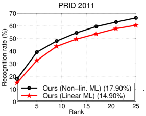
There exist several challenging benchmark data sets for person re-identification. In this experiment, we select four commonly used data sets (iLIDS, 3DPES, PRID2011, VIPeR) and two recently introduced data sets with a large number of individuals (CUHK01 and CUHK03). The iLIDS data set has $119$ individuals captured from eight cameras with different viewpoints [42]. The number of images for each individual varies from $2$ to $8$, i.e., eight cameras are used to capture $119$ individuals. The data set consists of large occlusions caused by people and luggages. The 3DPeS data set is designed mainly for people tracking and person re-identification [1]. It contains numerous video sequences taken from a real surveillance environment with eight different surveillance cameras and consists of $192$ individuals. The number of images for each individual varies from $2$ to $26$ images. The Person RE-ID 2011 (PRID2011) data set consists of images extracted from multiple person trajectories recorded from two surveillance static cameras [13]. Camera view A contains $385$ individuals, camera view B contains $749$ individuals, with $200$ of them appearing in both views. Hence, there are $200$ person image pairs in the dataset.

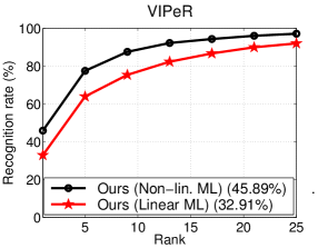
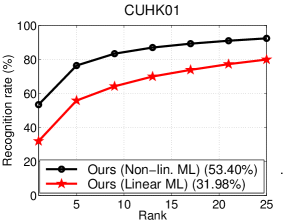
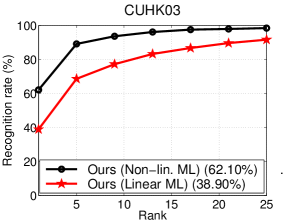
VIPeR is one of the most popular used data sets for person re-identification [11]. It conntains $632$ individuals taken from two cameras with arbitrary viewpoints and varying illumination conditions. The CUHK01 data set contains $971$ persons captured from two camera views in a campus environment [19]. Camera view A captures the frontal or back view of the individuals while camera view B captures the profile view. Finally, the CUHK03 data set consists of $1360$ persons taken from six cameras [20] The data set consists of manually cropped pedestrian images and images cropped from the pedestrian detector of [7]. Due to the imperfection in the pedestrian detector, which causes some misalignments of cropped images, we use images which are manually annotated by hand.

Figure 1: Performance comparison of base metrics with different visual features: SIFT$/$LAB, LBP$/$RGB, covariance descriptor and CNN features. Rank-$1$ recognition rates are shown in parentheses. The higher the recognition rate, the better the performance. Ours-Top (CMC${}^{\,\rm top}$) represents our ensemble approach which optimizes the CMC score over the top $k$ returned candidates. Ours-Triplet (CMC${}^{\,\rm triplet}$) represents our ensemble approach which minimizes the number of returned candidates such that the rank-$k$ recognition rate is equal to one.

Figure 2: Performance comparison of CMC${}^{\,\rm top}$ with two different base metrics: linear base metric (Linear Metric Learning) and non-linear base metric (Non-lin. Metric Learning). On VIPeR, CUHK01 and CUHK03 data sets, an ensemble of non-linear base metrics significantly outperforms an ensemble of linear base metrics.

Evaluation protocol

In this paper, we adopt a single-shot experiment setting, similar to [21, 26, 38, 41, 43]. For all data sets except CUHK03, all the individuals in the data set are randomly divided into two subsets so that the training set and the test set contains half of the available individuals with no overlap on person identities. For data set with two cameras, we randomly select one image of the individual taken from camera view A as the probe image and one image of the same individual taken from camera view B as the gallery image. For multi-camera data sets, two images of the same individual are chosen: one is used as the probe image and the other as the gallery image. For CUHK03, we set the number of individuals in the train$/$test split to $1260$$/$$100$ as conducted in [20]. To be more specific, there are $59$, $96$, $100$, $316$, $485$ and $100$ individuals in each of the test split for the iLIDS, 3DPeS, PRID2011, VIPeR, CUHK01 and CUHK03 data sets, respectively. The number of probe images (test phase) is equal to the number of gallery images in all data sets except PRID2011, in which the number of probe images is $100$ and the number of test gallery images is $649$ (all images from camera view B except the $100$ training samples). This procedure is repeated $10$ times and the average of cumulative matching charateristic (CMC) curves across $10$ partitions is reported. The CMC curve provides a ranking for every image in the gallery with respect to the probe.

Parameters setting

For the linear base metric (KISS ML [17]), we apply principal component analysis (PCA) to reduce the dimensionality and remove noise. Without performing PCA, it is computationally infeasible to inverse covariance matrices of both similar and dissimilar pairs as discussed in [17]. For each visual feature, we reduce the feature dimension to $64$ dimensional subspaces. For the non-linear base metric (kLFDA [38]), we set the regularization parameter for class scatter matrix to $0.01$, i.e., we add a small identity matrix to the class scatter matrix. For both SIFT$/$LAB and LBP$/$RGB features, we apply the RBF-$\chi^{2}$ kernel. For region covariance and CNN features, we apply the Gaussian RBF kernel $\kappa({\boldsymbol{x}},{\boldsymbol{x}}^{\prime})=\exp(-\|{\boldsymbol{x}}-{\boldsymbol{x}}^{\prime}\|/\sigma^{2})$. The kernel parameter is tuned to an appropriate value for each data set. In this experiment, we set the value of $\sigma^{2}$ to be the same as the first quantile of all distances [38].

For CMC${}^{\,\rm triplet}$, we choose the regularization parameter ($\nu$ in (1)) from $\{10^{3}$,$10^{3.1}$,$\cdots$,$10^{4}\}$ by cross-validation on the training data. For CMC${}^{\,\rm top}$, we choose the regularization parameter ($\nu$ in (7)) from $\{10^{2}$,$10^{2.1}$,$\cdots$,$10^{3}\}$ by cross-validation on the training data. We set the cutting-plane termination threshold to $10^{-6}$. The recall parameter ($k$ in (6)) is set to be $10$ for iLIDS, 3DPeS, PRID2011 and VIPeR and $40$ for larger data sets (CUHK01 and CUHK03). Since the success of metric learning algorithms often depends on the choice of good parameters, we train multiple metric learning for each feature. Specifically, for KISS ML, we reduce their feature dimensionality to $32$, $48$ and $64$ dimensions and use all three to learn the weight ${\boldsymbol{w}}$ for CMC${}^{\,\rm triplet}$ and CMC${}^{\,\rm top}$. Similarly, for kFLDA, we set the $\sigma^{2}$ to be the same as the 5, the 10 and the first quantile of all distances.

3.1 Evaluation and analysis

Feature evaluation

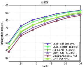
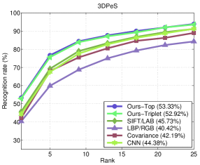
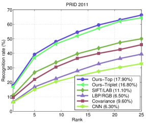
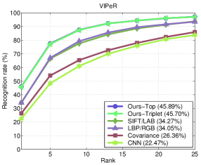
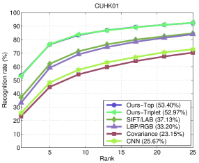
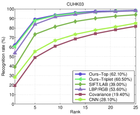
We investigate the impact of low-level and high-level visual features on the recognition performance of person re-identification. Fig. 1 shows the CMC performance of different visual features and their rank-$1$ recognition rates when trained with the kernel-based LFDA (non-linear metric learning) on six benchmark data sets. On VIPeR, CUHK01 and CUHK03 data sets, we observe that both SIFT$/$LAB and LBP$/$RGB significantly outperform covariance descriptor and CNN features. This result is not surprising since SIFT$/$LAB combines edges and color features while LPB$/$RGB combines texture and color features. We suspect the use of color helps improve the overall recognition performance of both features. We observe that CNN features perform poorer than hand-crafted low-level features in our experiments. We suspect that the CNN pre-trained model has been designed for ImageNet object categories [18], in which color information might be less important. However on many person re-id data sets, a large number of persons wear similar types of clothing, e.g., t-shirt and jeans, but with different color. Therefore color information becomes an important cue for recognizing two different individuals. Overall, we observe that SIFT$/$LAB features perform well consistently on all data sets evaluated.

Ensemble approach with different base metrics

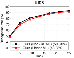
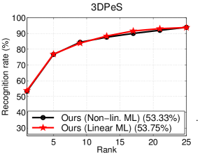
Next we compare the performance of our approach with two different base metrics: linear metric learning [17] and non-linear metric learning [38] (introduced in Sec. 2.2). In this experiment, we use CMC${}^{\,\rm top}$ to learn an ensemble. Experimental results are shown in Fig. 2. Two observations can be made from the figure: 1) Both approaches perform similarly when the number of train$/$test individuals is small, e.g., on iLIDS and 3DPeS data sets; 2) Non-linear base metrics outperforms linear base metric when the number of individuals increase. We suspect that there is less diversity when the number of individuals is small. No further improvement is observed when we replace linear base metrics with non-linear base metrics.

Rank	VIPeR			CUHK01			CUHK03
	Avg.	CMC${}^{\,\rm triplet}$	CMC${}^{\,\rm top}$	Avg.	CMC${}^{\,\rm triplet}$	CMC${}^{\,\rm top}$	Avg.	CMC${}^{\,\rm triplet}$	CMC${}^{\,\rm top}$
$1$	$44.9$	$45.7$	$\mathbf{45.9}$	$51.9$	$53.0$	$\mathbf{53.4}$	$57.4$	$60.5$	$\mathbf{62.1}$
$2$	$58.3$	$59.6$	$\mathbf{60.2}$	$63.3$	$64.1$	$\mathbf{64.3}$	$71.7$	$73.5$	$\mathbf{76.6}$
$5$	$76.3$	$77.1$	$\mathbf{77.5}$	$75.1$	$76.1$	$\mathbf{76.4}$	$85.9$	$87.8$	$\mathbf{89.1}$
$10$	$88.2$	$\mathbf{88.9}$	$\mathbf{88.9}$	$83.0$	$84.0$	$\mathbf{84.4}$	$93.1$	$93.5$	$\mathbf{94.3}$
$20$	$94.9$	$95.7$	$\mathbf{95.8}$	$89.4$	$\mathbf{90.7}$	$90.5$	$96.9$	$97.4$	$\mathbf{97.8}$
$50$	$99.4$	$\mathbf{99.5}$	$\mathbf{99.5}$	$95.9$	$\mathbf{96.4}$	$\mathbf{96.4}$	$99.5$	$\mathbf{99.7}$	$\mathbf{99.7}$
$100$	$99.9$	$\mathbf{100.0}$	$\mathbf{100.0}$	$\mathbf{98.6}$	$\mathbf{98.6}$	$\mathbf{98.6}$	$\mathbf{100.0}$	$\mathbf{100.0}$	$\mathbf{100.0}$

Table 1: Re-id recognition rate ($\%$) at different recall (rank). The best result is shown in boldface. Both CMC${}^{\,\rm top}$ and CMC${}^{\,\rm triplet}$ achieve similar performance when retrieving $\geq 50$ candidates.

Figure 3: CMC performance for VIPeR and CUHK01 data sets. The higher the recognition rate, the better the performance. Our approach outperforms all existing person re-id algorithms.

Data set	# Individuals		Prev. best	Ours
	train	test
iLIDS	$59$	$60$	$40.3\%$ [38]	$\mathbf{50.3\%}$
3DPeS	$96$	$96$	$\mathbf{54.2\%}$ [38]	$53.3\%$
PRID2011	$100$	$100$	$16.0\%$ [28]	$\mathbf{17.9\%}$
VIPeR	$316$	$316$	$43.4\%$ [41]	$\mathbf{45.9\%}$
CUHK01	$486$	$485$	$34.3\%$ [41]	$\mathbf{53.4\%}$
CUHK03	$1260$	$100$	$20.7\%$ [20]	$\mathbf{62.1\%}$

Table 2: Rank-$1$ recognition rate of existing best reported results and our results. The best result is shown in boldface.

Performance at different recall values

Next we compare the performance of the proposed CMC${}^{\,\rm triplet}$ with CMC${}^{\,\rm top}$. Both optimization algorithms optimize the recognition rate of person re-id but with different objective criteria. We compare the performance of both algorithms with the baseline approach, in which we simply set the value of ${\boldsymbol{w}}$ to a uniform weight. Since distance functions of different features have different scales, we normalize the distance between each probe image to all images in the gallery to be between zero and one. In other words, we set the distance between the probe image and the nearest gallery image to be zero and the distance between the probe image and the furthest gallery image to be one. The matching accuracy is shown in Table 1. We observe that CMC${}^{\,\rm top}$ achieves the best recognition rate performance at a small recall value. At a large recall value (rank $\geq 50$), both CMC${}^{\,\rm top}$ and CMC${}^{\,\rm triplet}$ perform similarly. Interestingly, a simple averaging performs quite well on VIPeR, in which the number of individuals in the test set is small.

3.2 Comparison with state-of-the-art results

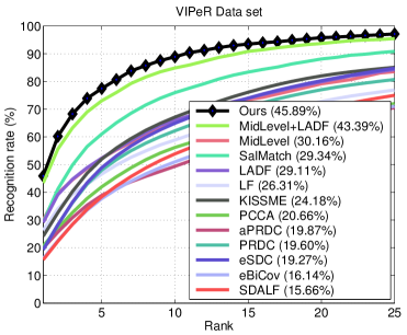
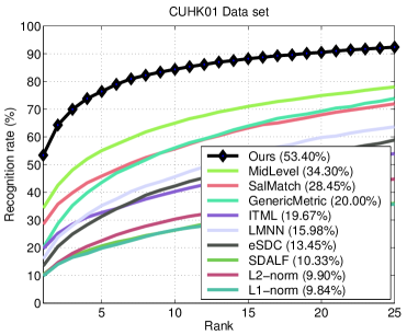
Fig. 3 compares our results with other person re-id algorithms on two major benchmark data sets: VIPeR and CUHK01. Our approach outperforms all existing person re-id algorithms. Next we compare our results with the best reported results in the literature. The algorithm proposed in [38] achieves state-of-the-art results on iLIDS and 3DPeS data sets ($40.3\%$ and $54.2\%$ recognition rate at rank-$1$, respectively). Our approach outperforms [38] on the iLIDS ($50.3\%$) and achieve a comparable result on 3DPeS ($53.3\%$). Zhao et al. propose mid-level filters for person re-identification [41], which achieve state-of-the-art results on the VIPeR and CUHK01 data sets ($43.39\%$ and $34.30\%$ recognition rate at rank-$1$, respectively). Our approach outperforms [41] by achieving a recognition rate of $45.89\%$ and $53.40\%$ on the VIPeR and CUHK01 data sets, respectively. Table 2 compares our results with other state-of-the-art methods on other person re-identification data sets.

4 Conclusion

In this paper, we present an effective structured learning based approach for person re-id by combining multiple low-level and high-level visual features into a single framework. Our approach is practical to real-world applications since the performance can be concentrated in the range of most practical importance. Moreover our proposed approach is flexible and can be applied to any metric learning algorithms. Experimental results demonstrate the effectiveness of the proposed approach on six major person re-id data sets.

References

- [1] D. Baltieri, R. Vezzani, and R. Cucchiara. 3DPes: 3D people dataset for surveillance and forensics. In Proc. of Int’l. Workshop on Mult. Acc. to 3D Human Objs., 2011.
- [2] L. Bazzani, M. Cristani, A. Perina, and V. Murino. Multiple-shot person re-identification by chromatic and epitomic analyses. Patt. Recogn., 33(7):898–903, 2012.
- [3] D. S. Cheng, M. Cristani, M. Stoppa, L. Bazzani, and V. Murino. Custom pictorial structures for re-identification. In Proc. British Mach. Vis. Conf., 2011.
- [4] S. Chopra, R. Hadsell, and Y. LeCun. Learning a similarity metric discriminatively, with application to face verification. In Proc. IEEE Conf. Comp. Vis. Patt. Recogn., 2005.
- [5] J. V. Davis, B. Kulis, P. Jain, S. Sra, and I. S. Dhillon. Information-theoretic metric learning. In Proc. Int. Conf. Mach. Learn., 2007.
- [6] M. Farenzena, L. Bazzani, A. Perina, V. Murino, and M. Cristani. Person re-identification by symmetry-driven accumulation of local features. In Proc. IEEE Conf. Comp. Vis. Patt. Recogn., 2010.
- [7] P. Felzenszwalb, R. Girshick, D. McAllester, and D. Ramanan. Object detection with discriminatively trained part based models. IEEE Trans. Pattern Anal. Mach. Intell., 32(9):1627–1645, 2010.
- [8] A. Frome, Y. Singer, S. Fei, and J. Malik. Learning globally-consistent local distance functions for shape-based image retrieval and classification. In Proc. IEEE Int. Conf. Comp. Vis., 2007.
- [9] N. Gheissari, T. B. Sebastian, and R. Hartley. Person reidentification using spatiotemporal appearance. In Proc. IEEE Conf. Comp. Vis. Patt. Recogn., 2006.
- [10] S. Gong, M. Cristani, S. Yan, and C. C. Loy. Person Re-Identification. Springer, 2014.
- [11] D. Gray, S. Brennan, and H. Tao. Evaluating appearance models for recognition, reacquisition, and tracking. In Proc. Int’l. Workshop on Perf. Eval. of Track. and Surv’l., 2007.
- [12] D. Gray and H. Tao. Viewpoint invariant pedestrian recognition with an ensemble of localized features. In Proc. Eur. Conf. Comp. Vis., 2008.
- [13] M. Hirzer, C. Beleznai, P. M. Roth, and H. Bischof. Person re-identification by descriptive and discriminative classification. In Proc. Scandinavian Conf. on Image Anal., 2011.
- [14] M. Hirzer, P. Roth, and H. Bischof. Person re-identification by efficient imposter-based metric learning. In Proc. Int’l. Conf. on Adv. Vid. and Sig. Surveillance, 2012.
- [15] T. Joachims. A support vector method for multivariate performance measures. In Proc. Int. Conf. Mach. Learn., 2005.
- [16] D. Kedem, S. Tyree, F. Sha, G. R. Lanckriet, and K. Q. Weinberger. Non-linear metric learning. In Proc. Adv. Neural Inf. Process. Syst., 2012.
- [17] M. Kostinger, M. Hirzer, P. Wohlhart, P. M. Roth, and H. Bischof. Large scale metric learning from equivalence constraints. In Proc. IEEE Conf. Comp. Vis. Patt. Recogn., 2012.
- [18] A. Krizhevsky, I. Sutskever, and G. E. Hinton. Imagenet classification with deep convolutional neural networks. In Proc. Adv. Neural Inf. Process. Syst., 2012.
- [19] W. Li, R. Zhao, and X. Wang. Human reidentification with transferred metric learning. In Proc. Asian Conf. Comp. Vis., 2012.
- [20] W. Li, R. Zhao, T. Xiao, and X. Wang. Deepreid: Deep filter pairing neural network for person re-identification. In Proc. IEEE Conf. Comp. Vis. Patt. Recogn., 2014.
- [21] Z. Li, S. Chang, F. Liang, T. S. Huang, L. Cao, and J. R. Smith. Learning locally-adaptive decision functions for person verification. In Proc. IEEE Conf. Comp. Vis. Patt. Recogn., 2013.
- [22] D. G. Lowe. Distinctive image features from scale-invariant keypoints. Int. J. Comp. Vis., 60(2):91–110, 2004.
- [23] B. McFee and G. R. G. Lanckriet. Metric learning to rank. In Proc. Int. Conf. Mach. Learn., 2010.
- [24] H. Narasimhan and S. Agarwal. A structural svm based approach for optimizing partial auc. In Proc. Int. Conf. Mach. Learn., 2013.
- [25] T. Ojala, M. Pietikainen, and T. Maenpaa. Multiresolution gray-scale and rotation invariant texture classification with local binary patterns. IEEE Trans. Pattern Anal. Mach. Intell., 24(7):971–987, 2002.
- [26] S. Pedagadi, J. Orwell, S. Velastin, and B. Boghossian. Local fisher discriminant analysis for pedestrian re-identification. In Proc. IEEE Conf. Comp. Vis. Patt. Recogn., 2013.
- [27] B. Prosser, W. S. Zheng, S. Gong, T. Xiang, and Q. Mary. Person re-identification by support vector ranking. In Proc. British Mach. Vis. Conf., 2010.
- [28] P. M. Roth, M. Hirzer, M. Köstinger, C. Beleznai, and H. Bischof. Mahalanobis distance learning for person re-identification. In Person Re-Identification, pages 247–267. Springer, 2014.
- [29] M. Schultz and T. Joachims. Learning a distance metric from relative comparisons. In Proc. Adv. Neural Inf. Process. Syst., 2004.
- [30] W. Schwartz and L. Davis. Learning discriminative appearance-based models using partial least squares. In Proc. of SIBGRAPI, 2009.
- [31] J. Shawe-Taylor and N. Cristianini. Kernel Methods for Pattern Analysis. Cambridge University Press, 2004.
- [32] C. H. Teo, A. Smola, S. V. N. Vishwanathan, and Q. V. Le. A scalable modular convex solver for regularized risk minimization. In Proc. of Int. Conf. on Knowl. Disc. and Data Mining, 2007.
- [33] O. Tuzel, F. Porikli, and P. Meer. Region covariance: A fast descriptor for detection and classification. In Proc. Eur. Conf. Comp. Vis., 2006.
- [34] X. Wang, G. Doretto, T. Sebastian, J. Rittscher, and P. Tu. Shape and appearance context modeling. In Proc. IEEE Int. Conf. Comp. Vis., 2007.
- [35] K. Weinberger, J. Blitzer, and L. Saul. Distance metric learning for large margin nearest neighbor classification. In Proc. Adv. Neural Inf. Process. Syst., 2006.
- [36] K. Q. Weinberger and L. K. Saul. Fast solvers and efficient implementations for distance metric learning. In Proc. Int. Conf. Mach. Learn., 2008.
- [37] Y. Wu, M. Mukunoki, T. Funatomi, M. Minoh, and S. Lao. Optimizing mean reciprocal rank for person re-identification. In Advanced Video and Signal-Based Surveillance, 2011.
- [38] F. Xiong, M. Gou, O. Camps, and M. Sznaier. Person re-identification using kernel-based metric learning methods. In Proc. Eur. Conf. Comp. Vis., 2014.
- [39] L. Yang and R. Jin. Distance metric learning: A comprehensive survey. Michigan State Universiy, 2, 2006.
- [40] R. Zhao, W. Ouyang, and X. Wang. Unsupervised salience learning for person re-identification. In Proc. IEEE Conf. Comp. Vis. Patt. Recogn., 2013.
- [41] R. Zhao, W. Ouyang, and X. Wang. Learning mid-level filters for person re-identfiation. In Proc. IEEE Conf. Comp. Vis. Patt. Recogn., 2014.
- [42] W. Zheng, S. Gong, and T. Xiang. Associating groups of people. In Proc. British Mach. Vis. Conf., 2009.
- [43] W. S. Zheng, S. Gong, and T. Xiang. Person re-identification by probabilistic relative distance comparison. In Proc. IEEE Conf. Comp. Vis. Patt. Recogn., 2011.