Jointly Learning Multiple Measures of Similarities from Triplet Comparisons

Abstract

Similarity between objects is multi-faceted and it can be easier for human annotators to measure it when the focus is on a specific aspect. We consider the problem of mapping objects into view-specific embeddings where the distance between them is consistent with the similarity comparisons of the form “from the t-th view, object A is more similar to B than to C”. Our framework jointly learns view-specific embeddings exploiting correlations between views. Experiments on a number of datasets, including one of multi-view crowdsourced comparison on bird images, show the proposed method achieves lower triplet generalization error when compared to both learning embeddings independently for each view and all views pooled into one view. Our method can also be used to learn multiple measures of similarity over input features taking class labels into account and compares favorably to existing approaches for multi-task metric learning on the ISOLET dataset.

Introduction

Measure of similarity plays an important role in applications such as content-based recommendation, image search and speech recognition. Therefore a number of techniques to learn a measure of similarity from data have been proposed (?; ?; ?; ?). When the measure of distance is induced by an inner product in a low-dimensional space as is done in many studies, learning a distance metric is equivalent to learning an embedding of objects in a low-dimensional space. This is useful for visualization as well as using the learned representation in a variety of down-stream tasks that require fixed length representations of objects as has been demonstrated by the applications of word embeddings (?) in language.

Among various forms of supervision for learning distance metric, similarity comparison of the form ‘object $A$ is more similar to $B$ than to $C$”, which we call triplet comparison, is extremely useful for obtaining an embedding that reflects a perceptual similarity (?; ?; ?). Triplet comparisons can be obtained by crowdsourcing, or it may also be derived from class labels if available.

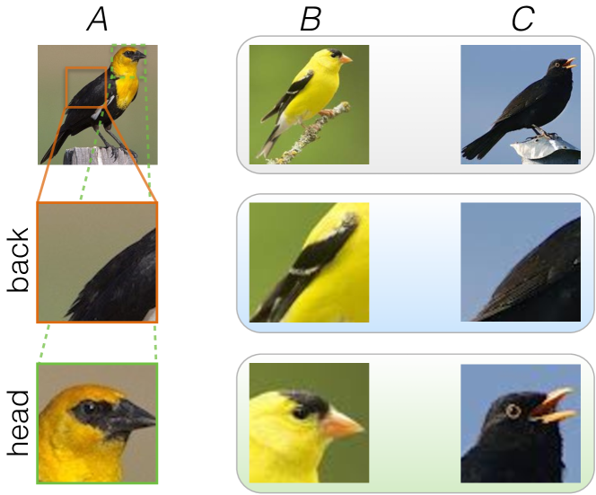
The task of judging similarity comparisons, however, can be challenging for human annotators. Consider the problem of comparing three birds as seen in Fig. 1. Most annotators will say that the head of bird $A$ is more similar to the head of $B$ while the back of $A$ is more similar to $C$. Such ambiguity leads to noise in annotation and results in poor embeddings.

A better approach would be to tell the annotator the desired view or the perspective of the object to use for measuring similarity. Such view-specific comparisons are not only easier for annotators, but they can also enable precise feedback for human “in the loop” tasks, such as, interactive fine-grained recognition (?), thereby reducing the human effort. The main drawback of learning view specific embeddings independently is that the number of similarity comparisons scales linearly with the number of views. This is undesirable as even learning a single embedding of $N$ objects may require $O(N^{3})$ triplet comparisons (?) in the worst case.

Figure 1: Ambiguity in similarity. Depending on whether we focus on the back (middle row) or on the head (bottom row), bird $A$ may appear more similar to $B$ or $C$.

We propose a method for learning embeddings jointly that addresses this drawback. Our method exploits underlying correlations that may exist between the views allowing a better use of the training data. Our method models the correlation between views by assuming that each view is a low-rank projection of a common embedding. Our model can be seen as a matrix factorization model in which local metric is defined as $\boldsymbol{L}\boldsymbol{M}_{t}\boldsymbol{L}^{\top}$, where $\boldsymbol{L}$ is a matrix that parametrizes the common embedding and $\boldsymbol{M}_{t}$ is a positive semidefinite matrix parametrizing the individual view. The model can be efficiently trained by alternately updating the view specific metric and the common embedding.

We experiment with a synthetic dataset and two realistic datasets, namely, poses of airplanes, and crowd-sourced similarities collected on different body parts of birds (CUB dataset; Welinder et al., ?). On most datasets our joint learning approach obtains lower triplet generalization error compared to the independent learning approach or naively pooling all the views into a single one, especially when the number of training triplets is limited. Furthermore, we apply our joint metric learning approach to the multi-task metric learning setting studied by (?) to demonstrate that our method can also take input features and class labels into account. Our method compares favorably to the previous method on ISOLET dataset.

Formulation

In this section, we first review the single view metric learning problem considered in previous work. Then we extend it to the case where there are multiple measures of similarity.

Metric learning from triplet comparisons

Given a set of triplets $\mathcal{S}=\{(i,j,k)\mid\text{object $i$ is more similar to object $j$ than object $k$}\}$ and possibly input features $\boldsymbol{x}_{1},\ldots,\boldsymbol{x}_{N}\in\mathbb{R}^{H}$, we aim to find a positive semidefinite matrix $\boldsymbol{M}\in\mathbb{R}^{H\times H}$ such that the pair-wise comparison of the distances induced by the inner product $\left\langle\boldsymbol{x},\boldsymbol{y}\right\rangle_{\boldsymbol{M}}=\boldsymbol{x}^{\top}\boldsymbol{M}\boldsymbol{y}$ parametrized by $\boldsymbol{M}$ (approximately) agrees with $\mathcal{S}$, i.e., $(i,j,k)\in\mathcal{S}\Rightarrow\|\boldsymbol{x}_{i}-\boldsymbol{x}_{j}\|_{\boldsymbol{M}}^{2}<\|\boldsymbol{x}_{i}-\boldsymbol{x}_{k}\|_{\boldsymbol{M}}^{2}$. If no input feature is given, we take $\boldsymbol{x}_{i}$ as the $i$th coordinate vector in $\mathbb{R}^{N}$, and learning $\boldsymbol{M}$, which would become $N\times N$, would correspond to finding embeddings of the $N$ objects in a Euclidean space with dimension equal to the rank of $\boldsymbol{M}$.

Mathematically the problem can be expressed as follows:

$$\min_{\begin{subarray}{c}\boldsymbol{M}\in\mathbb{R}^{H\times H},\\ \boldsymbol{M}\succeq 0\end{subarray}}\quad \!\!\!\!\!\sum_{(i,j,k)\in\mathcal{S}}\!\!\!\!\!\ell(\|\boldsymbol{x}_{i}-\boldsymbol{x}_{j}\|_{\boldsymbol{M}}^{2},\|\boldsymbol{x}_{i}-\boldsymbol{x}_{k}\|_{\boldsymbol{M}}^{2})+\gamma\text{tr}(\boldsymbol{M}),$$ (1)

where $\|\boldsymbol{x}-\boldsymbol{y}\|_{\boldsymbol{M}}^{2}=(\boldsymbol{x}-\boldsymbol{y})^{\top}\boldsymbol{M}(\boldsymbol{x}-\boldsymbol{y})$; the loss function can be, for example, logistic (?), or hinge, $\ell(d_{i,j},d_{i,k})=\max(1+d_{i,j}-d_{i,k},0)$ (?; ?; ?). Other choices of loss functions lead to crowd kernel learning (?), and $t$-distributed stochastic triplet embedding (t-STE) (?). Penalizing the trace of the matrix $\boldsymbol{M}$ can be seen as a convex surrogate for penalizing the rank (?; ?). $\gamma>0$ is a regularization parameter.

After the optimal $\boldsymbol{M}$ is obtained, we can find a low-rank factorization of $\boldsymbol{M}$ as $\boldsymbol{M}=\boldsymbol{L}\boldsymbol{L}^{\top}$ with $\boldsymbol{L}\in\mathbb{R}^{H\times D}$. This is particularly useful when no input feature is provided, because each row of $\boldsymbol{L}$, which is $N\times D$ in this case, corresponds to a $D$ dimensional embedding of each object.

Jointly learning multiple metrics

Now let’s assume that $T$ sets of triplets $\mathcal{S}_{1},\ldots,\mathcal{S}_{T}$ are available. This can be obtained by asking annotators to focus on a specific aspect when making pair-wise comparisons as in human in the loop tasks (?; ?). Alternatively, different measures of similarity can come from considering multiple related metric learning problems as in (?; ?).

While a simple approach to handle multiple similarities would be to parametrize each aspect or view by a positive semidefinite matrix $\boldsymbol{M}_{t}$, this would not induce any shared structure among the views. Our goal is to learn a global transformation $\boldsymbol{L}$ that maps the objects in a common $D$ dimensional space as well as local view-specific metrics $\boldsymbol{M}_{t}$ ($t=1,\ldots,T$).

To this end, we formulate the learning problem as follows:

$$\min_{\begin{subarray}{c}\boldsymbol{L}\in\mathbb{R}^{H\times D},\\ \boldsymbol{M}_{t}\in\mathbb{R}^{D\times D},\\ \boldsymbol{M}_{t}\succeq 0\,(t=1,\ldots,T)\end{subarray}} \!\!\sum_{t=1}^{T}\sum_{(i,j,k)\in\mathcal{S}_{t}}\!\!\!\!\!\varphi_{i,j,k}(\boldsymbol{L},\boldsymbol{M}_{t})$$

$$\quad+\gamma\sum_{t=1}^{T}{\rm tr}(\boldsymbol{M}_{t})+\beta\|\boldsymbol{L}\|_{F}^{2}\,,$$ (2)

where $\varphi_{i,j,k}(\boldsymbol{L},\boldsymbol{M}):=\ell\bigl{(}\|\boldsymbol{L}^{\top}(\boldsymbol{x}_{i}-\boldsymbol{x}_{j})\|_{\boldsymbol{M}}^{2},\|\boldsymbol{L}^{\top}(\boldsymbol{x}_{i}-\boldsymbol{x}_{k})\|_{\boldsymbol{M}}^{2}\bigr{)}$, and $\ell$ is a loss function as above. We use the hinge loss in the experiments in this paper, but the proposed framework readily generalizes to other loss functions proposed in literature (?; ?). Note again that when no input feature is provided, the global transformation matrix $\boldsymbol{L}$ becomes an $N\times D$ matrix that consists of $D$ dimensional embedding of the objects.

Intuitively the global transformation $\boldsymbol{L}$ plays the role of a bottleneck and forces the local metrics to share the common $D$ dimensional subspace because they are restricted in the form $\boldsymbol{L}\boldsymbol{M}_{t}\boldsymbol{L}^{\top}$.

The proposed model (2) includes various simpler models as special cases. First, if $\boldsymbol{L}$ is an $H\times H$ identity matrix, there is no sharing across different views and indeed the objective function will decompose into a sum of view-wise objectives; we call this independent learning. On the other hand, if we constrain all $\boldsymbol{M}_{t}$ to be equal, the same metric will apply to all the views and the learned metric will be essentially the same as learning a single shared metric as in Eq. (1) with $\mathcal{S}=\cup_{t=1}^{T}\mathcal{S}_{t}$; we call this pooled learning.

We employ regularization terms for both the local metric $\boldsymbol{M}_{t}$ and the global transformation matrix $\boldsymbol{L}$ in (2). The trace penalties ${\rm tr}(\boldsymbol{M}_{t})$ are employed to obtain low-rank matrices $\boldsymbol{M}_{t}$ as above. The regularization term on the norm of $\boldsymbol{L}$ is necessary to resolve the scale ambiguity. Although the above formulation has two hyperparameters $\beta$ and $\gamma$, we show below in Proposition 1 that the product $\beta\gamma$ is the only hyperparameter that needs to be tuned.

To minimize the objective (2), we update $\boldsymbol{M}_{t}$’s and $\boldsymbol{L}$ alternately. Both updates are (sub)gradient descent. The $\boldsymbol{M}_{t}$ update is followed by a projection onto the positive semi-definite (PSD) cone. Note that if we choose a convex loss function, e.g., hinge-loss, then it becomes a convex problem with respect to $\boldsymbol{M}_{t}$’s and $\boldsymbol{M}_{t}$’s can be optimized independently since they appear in disjoint terms. The algorithm is summarized in Algorithm 1.

Effective regularization term

The sum of the two regularization terms employed in (2) can be reduced into a single effective regularization term with only one hyperparameter $\sqrt{\beta\gamma}$ as we show in the following proposition (we give the proof in the supplementary material).

Proposition 1.

$$\!\!\min_{\begin{subarray}{c}\boldsymbol{L}\in\mathbb{R}^{H\times D},\\ \boldsymbol{M}_{1},\ldots,\boldsymbol{M}_{T}\in\mathbb{R}^{D\times D}\end{subarray}}\!\!\!\! \gamma\sum_{t=1}^{T}{\rm tr}(\boldsymbol{M}_{t})+\beta\|\boldsymbol{L}\|_{F}^{2}=2\sqrt{\beta\gamma}{\rm tr}\left(\sum_{t=1}^{T}\boldsymbol{K}_{t}\right)^{\frac{1}{2}},$$

$${\rm s.t.}\quad \boldsymbol{L}\boldsymbol{M}_{t}\boldsymbol{L}^{\top}=\boldsymbol{K}_{t}\,(\forall t)$$

where the power $1/2$ in the r.h.s. is the matrix square root.

As a corollary, we can always reduce or maintain the regularization terms in (2) without affecting the loss term by the rescaling $\boldsymbol{M}_{t}\leftarrow\boldsymbol{M}_{t}/\alpha^{2}$ and $\boldsymbol{L}\leftarrow\alpha\boldsymbol{L}$ with $\alpha=(\gamma\sum_{t=1}^{T}\operatorname{tr}(\boldsymbol{M}_{t})/(\beta\|\boldsymbol{L}\|_{F}^{2}))^{1/4}$.

Number of parameters

A simple parameter counting argument tells us that independently learning $T$ views requires to fit $O(DHT)$ parameters, where $H$ is the number of input dimension, which can be as large as $N$, $D$ is the embedding dimension, and $T$ is the number of views. On the other hand, our joint learning model has only $O(HD+D^{2}T)$ parameters. Thus when $D<H$, our model has much fewer parameters and enables better generalization, especially when the number of triplets is limited.

Efficiency

Reducing the dimension from $H$ to $D$ by the common transformation $\boldsymbol{L}$ is also favorable in terms of computational efficiency. The projection of $\boldsymbol{M}_{t}$ to the cone of $D\times D$ PSD matrices is much more efficient when $D\ll H$ compared to independently learning $T$ views.

Input: the number of objects $N$ (or input features $(\boldsymbol{x}_{i})_{i=1}^{N}$); dimension of embedding $D$; triplet constraints $\mathcal{S}_{t}$, $t=1,\ldots,T$; regularization parameters $\beta$, $\gamma$; the number of inner gradient updates $m_{\rm max}$

Output: Global transformation $\boldsymbol{L}$; PSD matrices $\{{\boldsymbol{M}_{t}}\}_{t=1}^{T}$

Initialize $\boldsymbol{L}$ randomly; initialize ${\boldsymbol{M}_{t}}$ as identity matrices;

while not converged do

       Update $\boldsymbol{L}$ using step-size $\eta=\eta_{0}/\sqrt{m}$ for $m_{\rm max}$ times as

$$\boldsymbol{L}\leftarrow\boldsymbol{L}-\eta\left\{\sum_{t=1}^{T}\sum_{\begin{subarray}{c}(i,j,k)\in\mathcal{S}_{t}\\ \end{subarray}}\nabla_{\boldsymbol{L}}\varphi_{i,j,k}(\boldsymbol{L},\boldsymbol{M}_{t})+2\beta\boldsymbol{L}\right\}$$

for  $t\in\{1,2,\dots,T\}$ do

             Update $\boldsymbol{M}_{t}$ using step-size $\eta=\eta_{0}/\sqrt{m}$ for $m_{\rm max}$ times by taking a gradient step

$$\!{\boldsymbol{M}_{t}}\leftarrow {\boldsymbol{M}_{t}}-\eta\left\{\!\!\sum_{(i,j,k)\in\mathcal{S}_{t}}\!\!\!\!\!\!\nabla_{{\boldsymbol{M}_{t}}}\varphi_{i,j,k}(\boldsymbol{L},\boldsymbol{M}_{t})+\gamma\boldsymbol{I}_{D}\right\}$$

and projecting ${\boldsymbol{M}_{t}}$ to the PSD cone;

            

       end for

      

end while

Algorithm 1 Multiple-metric Learning

Learning embeddings from triplet comparisons

In this section, we demonstrate the statistical efficiency of our model in both the triplet embedding (no input feature), and multi-task metric learning scenarios (with features).

Experimental setup

Figure 2: (Left) View-specific similarities between poses of planes were obtained by considering subsets of landmarks shown by different colored rectangles and measuring their similarity in configuration up to a scaling and translation. (Right) Perceptual similarities between bird species were collected by showing users either the full image (view $1$), or crops around various parts (view $2,3,4,5,6$). The average image for each view is also shown.

On each dataset, we divided the triplets into training and test and measured the quality of embeddings by the triplet generalization error, i.e., the fraction of test triplets whose relations are incorrectly modelled by the learned embedding. The error was measured for each view and averaged across views. The numbers of training triplets were the same for all the views. The regularization parameter was tuned using a 5-fold cross-validation on the training set with candidate values $\left\{10^{-5},10^{-4},\dots,10^{5}\right\}$. The hinge loss was used as the loss function. We use $m_{\rm max}=20$ as the number of inner iterations in the experiments.

In addition, we inspected how the similarity knowledge on existing views could be transferred to a new view where the number of similarity comparisons is small. We did this by conducting an experiment in which we drew a small set of training triplets from one view but used large numbers of training triplets from the other views.

We compared our method with the following two baselines. Independent: We conducted triplet embedding on each view treating each of them independently. We parametrized $\boldsymbol{M}=\boldsymbol{L}\boldsymbol{L}^{\top}$ with $\boldsymbol{L}\in\mathbb{R}^{N\times D}$ and minimized (1) using the software provided by van der Maaten and Weinberger (?). Pooled: We learned a single embedding with the training triplets from all the views combined.

Synthetic data

Description

Two synthetic datasets were generated. One consisted of 200 points uniformly sampled from a 10 dimensional unit hypercube, while the other dataset had 200 objects from a mixture of four Gaussian with variance 1 whose centers were randomly chosen in a hypercube with side length 10. Six views were generated on each dataset. Each view was produced by projecting data points onto a random subspace. The dimensions of the six random subspaces were 2, 3, 4, 5, 6, and 7 respectively.

Results

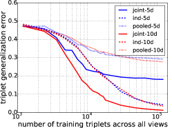
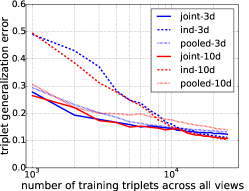
Embeddings were learned with embedding dimensions $D=5$ and 10. Triplet generalization errors are plotted in Fig. 3 (a) and (b) for clustered and uniform data, respectively. Our algorithm achieved lower triplet generalization error than both independent and pooled methods on both datasets. The improvement was particularly large when the number of triplets was limited (less than 10,000 for the clustered case). The simple pooled method was the worst on both datasets. Note that in contrast to the pooled method, the proposed joint method can choose different embedding dimension automatically (due to the trace regularization) for each view while maintaining a shared subspace.

(a) Clustered

(b) Uniform

(c) Poses of planes

Figure 3: Triplet generalization errors averaged across views for various datasets.

Poses of airplanes

Description

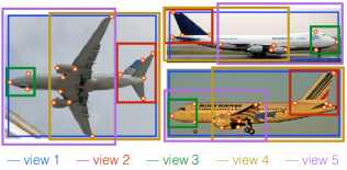
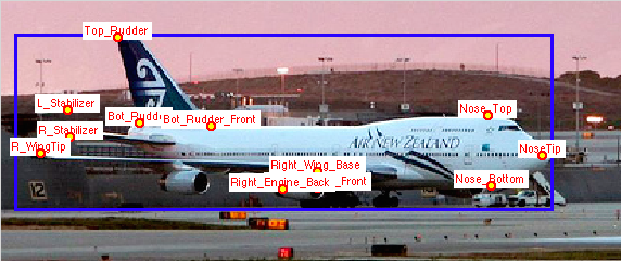
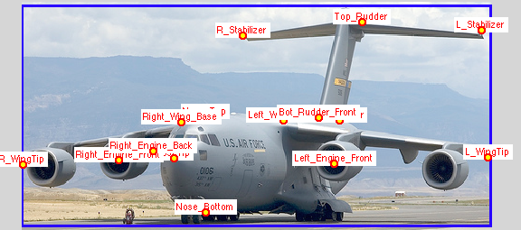
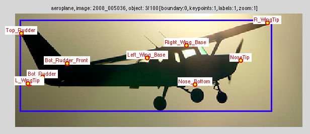
This dataset was constructed from 200 images of airplanes from the PASCAL VOC dataset (?) which were annotated with 16 landmarks such as nose tip, wing tips, etc (?). We used these landmarks to construct a pose-based similarity. Given two planes and the positions of landmarks in these images, pose similarity was defined as the residual error of alignment between the two sets of landmarks under scaling and translation. We generated 5 views each of which was associated with a subset of these landmarks; see supplementary material for details. Three annotated images from the set are shown in the left panel of Fig. 2. The planes are highly diverse ranging from passenger planes to fighter jets, varying in size and form which results in a slightly different similarity between instances for each view. However, there is a strong correlation between the views because the underlying set of landmarks are shared.

Results

We used $D=3$ and $D=10$ as embedding dimensions. Figure 3(c) shows the triplet generalization errors of the three methods. The proposed joint model performed clearly better than independent. This was not only in average but also uniformly for each view (see supplementary material). The pooled method had a slightly larger error than the proposed joint learning approach but better than the independent approach.

CUB-200 birds data

Description

We used the dataset (?) consisting of 200 species of birds and use the annotations collected using the setup of Wah et al. (?; ?). Briefly, similarity triplets among images of each species were collected in a crowd-sourced manner: every time, a user was asked to judge the similarity between an image of a bird from the target specie $z_{i}$ and nine images of birds of different species $\{z_{k}\}_{k\in\mathcal{K}}$ using the interface of Wilber et al. (?), where $\mathcal{K}$ is the set of all 200 species. For each display, the user partitioned these nine images into two sets, $\mathcal{K}_{sim}$ and $\mathcal{K}_{dissim}$, with $\mathcal{K}_{sim}$ containing birds considered similar to the target and $\mathcal{K}_{dissim}$ having the ones considered dissimilar. Such a partition was broadcast to an equivalent set of triplet constraints on associated species, $\{(i,j,l)\mid j\in\mathcal{K}_{sim},\,l\in\mathcal{K}_{dissim}\}$. Therefore, for each user response, $\left|\mathcal{K}_{sim}\right|\left|\mathcal{K}_{dissim}\right|$ triplet constraints were obtained.

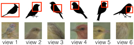
To collect view-specific triplets, we presented 5 different cropped versions (e.g. beak, breast, wing) of the bird images as shown in the right panel of Fig. 2 and used the same procedure as before to collect triplet comparisons. We obtained about 100,000 triplets from the uncropped original images and about 4,000 to 7,000 triplets from the 5 cropped views. This dataset reflects a more realistic situation where not all triplet relations are available and some of them may be noisy due to the nature of crowd-sourcing.

In addition to the triplet generalization error, we evaluated the embeddings in a classification task using a biological taxonomy of the bird species. Note that in Wah et al. (?) embeddings were used to interactively categorize images; here we simplify this process to enable detailed comparisons. We manually grouped the 200 classes to get 6 super classes so that the number of objects in all classes were balanced. These class labels were not used in the training but allowed us to evaluate the quality of embeddings using the leave-one-out (LOO) classification error. More precisely, at the test stage, we predict the class label of each embedded point according to the labels of its 3-nearest-neighbours (3-NN) in the learned metric.

Finally, since more triplets were available from the first (uncropped) view compared to other views, we first sampled equal numbers of triplets in each view up to a total of 18,000 triplets. Afterwards, we added triplets only to the first view.

Results

(a) Triplet generalization error

(b) LOO 3-NN classification error

(c) Learning a new view

Figure 4: Results on CUB-200 birds dataset. (c) shows the triplet generalization error on the second view.

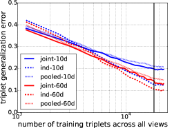
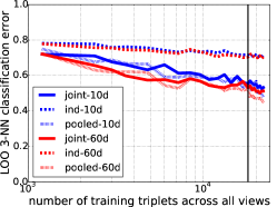
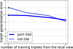
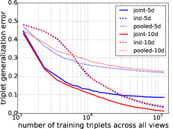
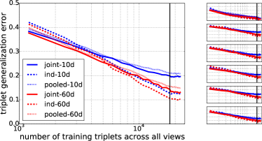
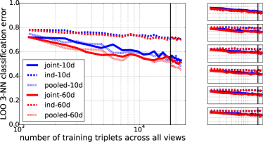
We used $D=10$ and $D=60$ as embedding dimensions; note that joint learning in 60 dimensions roughly has the same number of parameters as independent learning in 10 dimensions. Figures 4 (a) and (b) show the triplet generalization errors and the LOO 3-NN classification errors, respectively. The solid vertical line shows the point (18,000 triplets) that we start to add training triplets only to the first view. Comparing joint learning in 10 dimensions and 60 dimensions, we see that the higher dimension gives the lower error. The error of joint learning was better than independent learning for small number of triplets. Interestingly the error of joint learning in 60 dimensions coincides with that of independent learning in 10 dimensions after seeing 6,000 triplets. This can be explained by the fact that with 6 views, the two models have comparable complexity (see discussion at the end of the previous section) and thus the same asymptotic variance. Our method obtains lower leave-one-out classification errors on all views except for the first view; see supplementary material.

Learning a new view

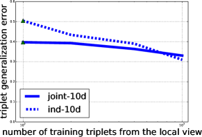
On the CUB-200 birds dataset, we simulated the situation of learning a new view (or zero-shot learning). We drew a training set that contains 100–1000 triplets from the second view and 3,000 triplets from all other 5 views. We investigated how joint learning helps in estimating a good embedding on a new view with extremely small number of triplets. The triplet generalization errors of both approaches are shown in Fig. 4(c). The triplet generalization error of the proposed joint learning was lower than that of the independent learning up to around 700 triplets. The embedding of the second view learned jointly with other views was clearly better than that learned independently and consistent with the quantitative evaluation; see supplementary material.

Performance gain and triplet consistency

In Fig. 5, we relate the performance gain we obtained for the joint/pooled learning approaches compared to the independent learning approach with the underlying between-task similarity. The performance gain was measured by the difference between the area under the triplet generalization errors normalized by that of the independent learning. The between-task similarity was measured by the triplet consistency between two views averaged over all pairs of views. For the CUB-200 dataset in which only a subset of valid triplet constraints are available, we take the independently learned embeddings with the largest number of triplets and use those to compute the triplet consistency.

We can see that when the triplet consistency is very high, pooled learning approach is good enough. However, when the triplet consistency is not too high, it may harm to pool the triplets together. The proposed joint learning approach has the most advantage in this intermediate regime. On the other hand, the consistency was close to random (0.5) for the CUB-200 dataset possibly explaining why the performance gain was not as significant as in the other datasets.

Figure 5: Relating the performance gains of joint and pooled learning with the triplet consistency.

Incorporating features and class information

The proposed method can be applied to a more general setting in which each object comes with a feature vector and a loss function not derived from triplet constraints is used.

Table 1: Test error rates on ISOLET dataset.

	Tested with view-specific train data			Tested with all train data
Task	MT-LMNN	Proposed method		MT-LMNN	Proposed method
	378 dim	$D=169$	$D=378$	378 dim	$D=169$	$D=378$
1	4.68	3.78	4.10	4.23	3.46	3.65
2	4.55	3.91	3.52	3.14	3.84	3.40
3	6.28	5.32	5.64	3.52	3.39	3.52
4	7.76	5.83	5.83	4.23	4.10	3.52
5	6.28	5.06	5.19	4.23	3.97	3.97
Avg	5.91	4.78	4.86	3.87	3.76	3.61

As an example, we employ the idea of multi-task large margin nearest neighbor (MT-LMNN) algorithm (?) and adapt our model to handle a classification problem. The loss function of MT-LMNN consists of two terms. The first term is a hinge loss for triplet constraints as in (2) but the triplets are derived from class labels. The second term is the sum of squared distances between each object and its “target neighbors” which is also defined based on class labels; see Weinberger et al. (?; ?) for details. The major difference between MT-LMNN and our model is that MT-LMNN parametrizes a local metric as the sum of a global average $\boldsymbol{M}_{0}$ and a view-specific metric $\boldsymbol{M}_{t}$ as $\boldsymbol{K}_{t}=\boldsymbol{M}_{0}+\boldsymbol{M}_{t}$; thus the learned metric is generally full rank. On the other hand, our method parametrizes it as a product of global transform and local metric as $\boldsymbol{K}_{t}=\boldsymbol{L}\boldsymbol{M}_{t}\boldsymbol{L}^{\top}$, which allows the local embedding dimension to be controlled by the trace regularization.

We conduct experiments on ISOLET spoken alphabet recognition dataset (?) which consists 7797 examples of English alphabets spoken by 150 subjects and each example is described by a 617 dimension feature vector. The task is to recognize the letter of each spoken example as one of the English alphabets. The subjects are grouped into sets of 30 similar speakers leading to 5 tasks.

We adapt the experimental setting from the work of MT-LMNN. Data is first projected onto its first 378 leading PCA components that capture 99 % of variance. We train our model in a $H=378$ dimensional space with $D=169$ and $378$, and compare it with a MT-LMNN trained with the code provided by the authors. In the experiment, each task is randomly divided into 60/20/20 subsets for train/validation/test. We tuned the parameters on the validation sets.

Test error rates of 3-nearest-neighbor (3-NN) classifiers are reported in Table 1. The left panel shows the errors using only the view-specific training data for the classification. The right panel shows those using all the training data with view-specific distance. Results are averaged over 10 runs. Simpler baseline methods, such as, euclidean metric and pooled (single task) learning are not included here because MT-LMNN already performed better than them. We can see that the proposed method performed better than MT-LMNN, while learning in a 378 dimensional space and reducing to a 169 dimensional space led to comparable error rates. A possible explanation for this mild dependence on the choice of embedding dimension $D$ could be given by the fact that both $\boldsymbol{L}$ and $\boldsymbol{M}_{t}$ are regularized and the effective embedding dimension is determined by the regularization and not by the choice of $D$; see Prop. 1. The averaged error rates reported in the original paper using 169 PCA dimensions were 5.19 % for the view-specific case and 4.01 % when all training data were used; our numbers are still better than theirs.

Related work

Embedding of objects from triplet or paired distance comparisons goes back to the work of Shepard (?; ?) and Kruskal (?; ?) and studied extensively (?; ?; ?; ?; ?) recently.

More recently, triplet embedding / metric learning problems that involve multiple measures of similarity have been considered. Parameswaran and Weinberger (?) aimed at jointly solving multiple related metric learning problems by exploiting possible similarities. More specifically, they modeled the inner product in each view by a sum of shared global matrix and a view-specific local matrix. Moreover, Rai, Lian, and Carin (?) proposed a Bayesian approach to multi-task metric learning. Unfortunately, the sum structure in their work typically do not produce a low-rank metric, which makes it unsuitable for learning view-specific embeddings. In contrast, our method models it as a product of them allowing the trace norm regularizer to determine the rank of each local metric. Xie and Xing (?) and Yu, Wang, and Tao (?) studied metric learning problems with multiple input views. This is different from our setting in which the notion of similarity varies from view to view. Amid and Ukkonen (?) considered the task of multi-view triplet embedding in which the view is a latent variable; they proposed a greedy algorithm for finding the view membership of each object as well as its embedding. It could be useful to combine this approach with ours when we do not have enough resource to collect triplets from all possible views.

Discussion

We have proposed a model for jointly learning multiple measures of similarities from multi-view triplet observations. The proposed model consists of a global transformation, which represents each object as a fixed dimensional vector, and local view-specific metrics.

Experiments on both synthetic and real datasets have demonstrate that our proposed joint model outperforms independent and pooled learning approaches in most cases. Additionally, we have shown that the advantage of our joint learning approach becomes the most prominent when the views are similar but not too similar (which can be measured by triplet consistency). Morevoer, we have extended our model to incorporate class labels and feature vectors. The proposed model performed favorably compared to MT-LMNN on ISOLET dataset. Since in many real applications, similarity triplets can be expensive to obtain, jointly learning similarity metrics is preferable as it can recover the underlying structure using relatively small number of triplets.

One way to look at the proposed model is to view the shared global transformation as controlling the complexity. However our experiments have shown that generally the higher the dimension, the better the performance (except for the ISOLET dataset tested with view-specific training data). Thus an alternative explanation could be that the regularization on both the global transformation $\boldsymbol{L}$ and local metrics $\boldsymbol{M}_{t}$ is implicitly controlling the embedding dimension.

Future work includes extension of the current model to other loss functions (e.g., the t-STE loss (?)) and to the setting in which we do not know which view each triplet came from.

Proof of Proposition 1

We repeat the statement for convenience.

Proposition 1.

$$\min_{\begin{subarray}{c}\boldsymbol{L}\in\mathbb{R}^{H\times D},\\ \boldsymbol{M}_{1},\ldots,\boldsymbol{M}_{T}\in\mathbb{R}^{D\times D}\end{subarray}}\left(\gamma\sum_{t=1}^{T}{\rm tr}(\boldsymbol{M}_{t})+\beta\|\boldsymbol{L}\|_{F}^{2}:\,\boldsymbol{L}\boldsymbol{M}_{t}\boldsymbol{L}^{\top}=\boldsymbol{K}_{t}\,(\forall t)\right)=2\sqrt{\beta\gamma}{\rm tr}\left(\sum\nolimits_{t=1}^{T}\boldsymbol{K}_{t}\right)^{1/2}$$

Here the power $1/2$ in the right-hand side is the matrix square root.

Proof.

Let’s define $\bar{\boldsymbol{M}}=\sum_{t=1}^{T}\boldsymbol{M}_{t}$. For any decomposition $\boldsymbol{K}_{t}=\boldsymbol{L}\boldsymbol{M}_{t}\boldsymbol{L}^{\top}$, we have

$$2\sqrt{\beta\gamma}{\rm tr}\left(\sum_{t=1}^{T}\boldsymbol{K}_{t}\right)^{1/2} =2\sqrt{\beta\gamma}{\rm tr}\left(\boldsymbol{L}\bar{\boldsymbol{M}}\boldsymbol{L}^{\top}\right)^{1/2}$$

$$=2\sqrt{\beta\gamma}\|\bar{\boldsymbol{M}}^{1/2}\boldsymbol{L}\|_{\ast}$$

$$=2\sqrt{\beta\gamma}\sum_{j=1}^{r}\sigma_{j}(\bar{\boldsymbol{M}}^{1/2}\boldsymbol{L})$$

$$\leq 2\sqrt{\beta\gamma}\sum_{j=1}^{r}\sigma_{j}(\bar{\boldsymbol{M}}^{1/2})\sigma_{j}(\boldsymbol{L})$$

$$\leq\sum_{j=1}^{r}\left(\gamma\sigma_{j}^{2}(\bar{\boldsymbol{M}}^{1/2})+\beta\sigma_{j}^{2}(\boldsymbol{L})\right)$$

$$=\gamma{\rm tr}(\bar{\boldsymbol{M}})+\beta\|\boldsymbol{L}\|_{F}^{2},$$

$$=\gamma\sum_{t=1}^{T}{\rm tr}(\boldsymbol{M}_{t})+\beta\|\boldsymbol{L}\|_{F}^{2}$$

where $\|\cdot\|_{\ast}$ is the nuclear norm (?); the fourth line follows from Theorem 3.3.14 (a) in Horn & Johnson (?), and the fifth line is due to the arithmetic mean-geometric mean inequality.

Let $\bar{\boldsymbol{K}}:=\sum_{t=1}^{T}\boldsymbol{K}_{t}$ and $\bar{\boldsymbol{K}}=\boldsymbol{U}\boldsymbol{\Lambda}\boldsymbol{U}^{\top}$ be its eigenvalue decomposition. The equality is achieved by choosing

$$\boldsymbol{L} =\boldsymbol{U}\boldsymbol{\Lambda}^{1/4}(\gamma/\beta)^{1/4}$$ (3)

$$\boldsymbol{M}_{t} =\boldsymbol{\Lambda}^{-1/4}\boldsymbol{U}^{\top}\boldsymbol{K}_{t}\boldsymbol{U}\boldsymbol{\Lambda}^{-1/4}(\beta/\gamma)^{1/2}\quad(t=1,\ldots,T)$$ (4)

Note that even when $\bar{\boldsymbol{K}}$ is singular, $\boldsymbol{K}_{t}$ is spanned by $\bar{\boldsymbol{K}}$ and by restricting to the subspace spanned by $\bar{\boldsymbol{K}}$, the above discussion is still valid. ∎

This lemma can be understood analogously to the identity regarding the nuclear norm(?)

$$\|\boldsymbol{X}\|_{\ast}=\min_{\boldsymbol{U},\boldsymbol{V}}\frac{1}{2}\left(\|\boldsymbol{U}\|_{F}^{2}+\|\boldsymbol{V}\|_{F}^{2}\right)\quad\text{subject to}\quad\boldsymbol{X}=\boldsymbol{U}\boldsymbol{V}^{\top}.$$

Note that the fact that the ratio of the two hyperparameters $\beta/\gamma$ can be absorbed in the scale ambiguity between $\boldsymbol{L}$ and $\boldsymbol{M}_{t}$ as in (3) and (4) is special to multiplicative models like our model and the nuclear norm and would not hold for an additive model like MT-LMNN.

Additional details and results

Synthetic dataset

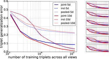
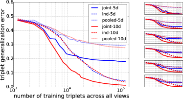
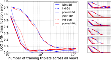
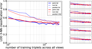
In addition to the results in main paper, we illustrate view-specific triplet generalization error in Figure 6 and leave-one-out classification error for clustered synthetic data in Figure 7.

Figure 6: Triplet generalization errors. The small figures shows errors on individual views and the large figures show the average. (Left) Clustered synthetic data. (Right) Uniformly distributed data.

Figure 7: Leave-one-out 3-nearest-neighbour classification errors on clustered synthetic data. The small figures shows errors on individual views and the large figures show the average.

Poses of airplanes dataset

Details of annotations and view generation

Each of the 200 airplanes were annotated with 16 landmarks namely,

01. Top_Rudder	05. L_WingTip	09. Nose_Bottom	13. Left_Engine_Back
02. Bot_Rudder	06. R_WingTip	10. Left_Wing_Base	14. Right_Engine_Front
03. L_Stabilizer	07. NoseTip	11. Right_Wing_Base	15. Right_Engine_Back
04. R_Stabilizer	08. Nose_Top	12. Left_Engine_Front	16. Bot_Rudder_Front

This is also illustrated in the Figure 8. The five different views are defined by considering different subsets of landmarks as follows:

1. all $\in\{1,2,\ldots,20\}$

2. back $\in\{1,2,3,4,16\}$

3. nose $\in\{7,8,9\}$

4. back+wings $\in\{1,2,\ldots,6,10,11,\ldots,16\}$

5. nose+wings $\in\{5,6,\ldots,15\}$

Figure 8: Landmarks illustrated on the several planes

For triplet $(A,B,C)$ we compute similarity $s_{i}(A,B)$ and $s_{i}(A,C)$ by aligning the subset $i$ of landmarks of $B$ and $C$ to $A$ under a translation and scaling that minimizes the sum of squared error after alignment. The similarity is inversely proportional to the residual error. This is also known as “procrustes analysis” commonly used for matching shapes.

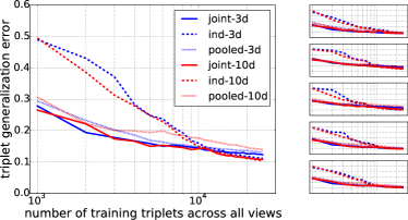
In addition to the results in main paper, we illustrate view-specific triplet generalization error and leave-one-out 3-nearest-neighbour classification error in Figure 9.

Figure 9: Experimental results on poses of planes dataset. The small figures shows errors on individual views and the large figures show the average. (Left) Triplet generalization errors on poses of planes dataset. (Right) Leave-one-out 3-nearest-neighbour classification error.

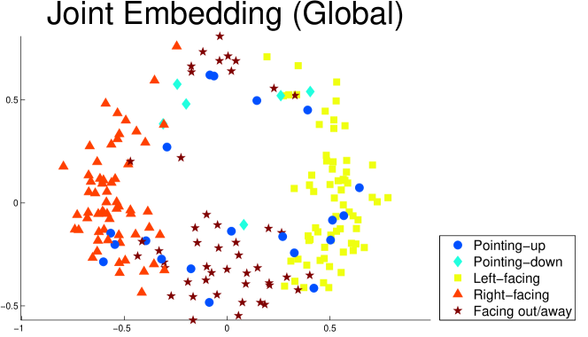
Learned embedding

Figure 10 shows a 2D projection of the global view of the objects onto their first two principle dimensions. The visualization shows that objects roughly lies on a circle corresponding to the left-right and up-down orientation.

Figure 10: The global view of embeddings of poses of planes.

CUB-200 birds dataset

Here, we also include the view-specific generalization errors and leave-one-out classification errors for CUB-200 Birds Dataset. See Figure 11.

Figure 11: Results on CUB-200 birds dataset. The small figures shows errors on individual views and the large figures show the average. (a) triplet generalization error. (b) leave-one-out 3-nearest-neighbor classification error.

Public figures face dataset

Description

Public Figures Face Database is created by Kumar et al.(?). It consists of 58,797 images of 200 people. Every image is characterized by 75 attributes which are real valued and describe the appearance of the person in the image. We selected 39 of the attributes and categorized them into 5 groups according to the aspects they describe: hair, age, accessory, shape and ethnicity. We randomly selected ten people and drew 20 images for each of them to create a dataset with 200 images. Similarity between instances for a given group is equal to the dot product between their attribute vectors where the attributes are restricted to those in the group. We describe the details of these attributes below. Each group is considered as a local view and identities of the people in the images are considered as class labels.

Attributes

Each image in the Public Figures Face Dataset (Pubfig) is characterized by 75 attributes. We used 39 of the attributes in our work and categorized them into 5 groups according to the aspects they describe. Here is a table of the categories and attributes:

Category	Attributes
Hair	Black Hair, Blond Hair, Brown Hair, Gray Hair, Bald, Curly Hair, Wavy Hair, Straight Hair, Receding Hairline, Bangs, Sideburns.
Age	Baby,Child,Youth,Middle Aged,Senior.
Accessory	No Eyewear, Eyeglasses, Sunglasses, Wearing Hat, Wearing Lipstick, Heavy Makeup, Wearing Earrings, Wearing Necktie, Wearing Necklace.
Shape	Oval Face, Round Face, Square Face, High Cheekbones, Big Nose, Pointy Nose, Round Jaw, Narrow Eyes, Big Lips, Strong Nose-Mouth Lines.
Ethnicity	Asian, Black, White, Indian.

Table 2: List of Pubfig attributes that were used in our work.

Results

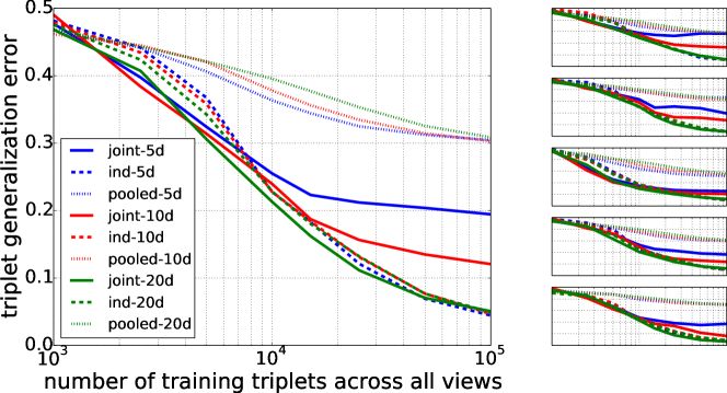
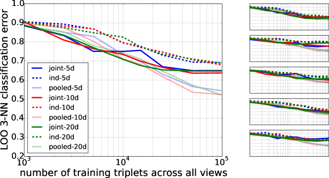
The 200 images are embedded into 5, 10, and 20 dimensional spaces. We draw triplets randomly from the ground truth similarity measure to form training and test sets. Triplet generalization errors and classification errors are shown in Fig. 12.

In terms of the triplet generalization error, the joint learning reduces the error faster than the independent learning up to around 10,000 triplets where the decrease slows down. Since the error in this regime reduces monotonically with increasing number of dimensions, this can be understood as a bias induced by the joint learning. On the other hand, when we have less than 10,000 triples, the error of the joint learning increases (but not as large as the independent learning) as dimension increases; this can be understood as a variance. When embedding in a 20 dimensional space, the joint learning has lower or comparable error to independent learning even when $10^{5}$ triplets are available. In terms of the leave-one-out classification error, joint learning continues to be better even when the number of triplets are very large.

Figure 12: Results on public figures faces dataset. Embeddings are learned in a 5 dimensional space, a 10 dimensional space and a 20 dimensional space. (a) Triplet generalization error. (b) Leave-one-out 3-nearest-neighbor classification error. The small figures shows errors on individual views and the large figures show the average.

Learning a new view

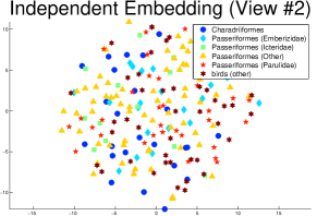
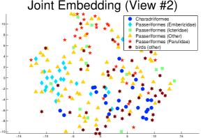
Figure 13 shows a 2D projection of the embeddings learned by the independent approach and the proposed joint approach in the setting for CUB-200 birds dataset described in the part of “learning a new view” in the main text. Clearly the proposed joint learning approach obtains a better separated clusters compared to the independent approach.

Figure 13: Learning a new view on CUB-200 birds dataset. Training data contains 100 triplets from the second local view and 3,000 triplets from other 5 views. Embeddings are learned in a 10 dimensional space and then further embedded in a 2 dimensional plane by using tSNE (?) for the purpose of visualization. Left: triplet generalization error on the second local view. Middle: embedding learned independently. Right: embedding learned jointly.

Relating the performance gain with the triplet consistency

Table 3: Relating the performance gain of joint and pooled learning with the between-task similarity.

	CUB-200	PubFig	Synthetic (uniform)	Synthetic (clustered)	Airplanes
Average triplet consistency	0.53	0.59	0.6	0.69	0.85
Performance gain of joint learning(%)	-4.6	6.5	26	44	35
Performance gain of pooled learning(%)	-8.0	-56	-40	-29	23

References

- [Agarwal et al. 2007] Agarwal, S.; Wills, J.; Cayton, L.; Lanckriet, G.; Kriegman, D. J.; and Belongie, S. 2007. Generalized non-metric multidimensional scaling. In International Conference on Artificial Intelligence and Statistics, 11–18.
- [Amid and Ukkonen 2015] Amid, E., and Ukkonen, A. 2015. Multiview triplet embedding: Learning attributes in multiple maps. In Proceedings of the 32nd International Conference on Machine Learning (ICML-15), 1472–1480.
- [Bourdev et al. 2010] Bourdev, L.; Maji, S.; Brox, T.; and Malik, J. 2010. Detecting people using mutually consistent poselet activations. In European Conference on Computer Vision (ECCV).
- [Chechik et al. 2010] Chechik, G.; Sharma, V.; Shalit, U.; and Bengio, S. 2010. Large scale online learning of image similarity through ranking. J. Mach. Learn. Res. 11:1109–1135.
- [Cox et al. 2000] Cox, I. J.; Miller, M. L.; Minka, T. P.; Papathomas, T. V.; and Yianilos, P. N. 2000. The bayesian image retrieval system, pichunter: theory, implementation, and psychophysical experiments. Image Processing, IEEE Transactions on 9(1):20–37.
- [Davis et al. 2007] Davis, J. V.; Kulis, B.; Jain, P.; Sra, S.; and Dhillon, I. S. 2007. Information-theoretic metric learning. In Proceedings of the 24th international conference on Machine learning, 209–216. ACM.
- [Everingham et al. 2010] Everingham, M.; Van Gool, L.; Williams, C. K. I.; Winn, J.; and Zisserman, A. 2010. The pascal visual object classes (voc) challenge. International Journal of Computer Vision 88(2):303–338.
- [Fanty and Cole 1991] Fanty, M. A., and Cole, R. A. 1991. Spoken letter recognition. In Adv. Neural. Inf. Process. Syst. 3, 220–226.
- [Fazel, Hindi, and Boyd 2001] Fazel, M.; Hindi, H.; and Boyd, S. P. 2001. A Rank Minimization Heuristic with Application to Minimum Order System Approximation. In Proc. of the American Control Conference.
- [Horn and Johnson 1991] Horn, R. A., and Johnson, C. R. 1991. Topics in matrix analysis. Cambridge University Press.
- [Jamieson and Nowak 2011] Jamieson, K. G., and Nowak, R. D. 2011. Low-dimensional embedding using adaptively selected ordinal data. In Communication, Control, and Computing (Allerton), 2011 49th Annual Allerton Conference on, 1077–1084. IEEE.
- [Kruskal 1964a] Kruskal, J. B. 1964a. Multidimensional scaling by optimizing goodness of fit to a nonmetric hypothesis. Psychometrika 29(1):1–27.
- [Kruskal 1964b] Kruskal, J. B. 1964b. Nonmetric multidimensional scaling: a numerical method. Psychometrika 29(2):115–129.
- [Kumar et al. 2009] Kumar, N.; Berg, A. C.; Belhumeur, P. N.; and Nayar, S. K. 2009. Attribute and simile classifiers for face verification. In Computer Vision, 2009 IEEE 12th International Conference on, 365–372. IEEE.
- [McFee and Lanckriet 2009] McFee, B., and Lanckriet, G. 2009. Partial order embedding with multiple kernels. In Proceedings of the 26th Annual International Conference on Machine Learning, 721–728. ACM.
- [McFee and Lanckriet 2011] McFee, B., and Lanckriet, G. 2011. Learning multi-modal similarity. The Journal of Machine Learning Research 12:491–523.
- [Mikolov et al. 2013] Mikolov, T.; Chen, K.; Corrado, G.; and Dean, J. 2013. Efficient estimation of word representations in vector space. arXiv preprint arXiv:1301.3781.
- [Parameswaran and Weinberger 2010] Parameswaran, S., and Weinberger, K. Q. 2010. Large margin multi-task metric learning. In Advances in neural information processing systems, 1867–1875.
- [Rai, Lian, and Carin 2014] Rai, P.; Lian, W.; and Carin, L. 2014. Bayesian multitask distance metric learning. In NIPS 2014 Workshop on Transfer and Multitask Learning.
- [Shepard 1962a] Shepard, R. N. 1962a. The analysis of proximities: Multidimensional scaling with an unknown distance function. I. Psychometrika 27(2):125–140.
- [Shepard 1962b] Shepard, R. N. 1962b. The analysis of proximities: Multidimensional scaling with an unknown distance function. II. Psychometrika 27(3):219–246.
- [Srebro, Rennie, and Jaakkola 2005] Srebro, N.; Rennie, J. D. M.; and Jaakkola, T. S. 2005. Maximum-margin matrix factorization. In Saul, L. K.; Weiss, Y.; and Bottou, L., eds., Advances in NIPS 17. Cambridge, MA: MIT Press. 1329–1336.
- [Tamuz et al. 2011] Tamuz, O.; Liu, C.; Belongie, S.; Shamir, O.; and Kalai, A. T. 2011. Adaptively learning the crowd kernel. arXiv preprint arXiv:1105.1033.
- [van der Maaten and Hinton 2008] van der Maaten, L., and Hinton, G. 2008. Visualizing data using t-sne. Journal of Machine Learning Research 9(2579-2605):85.
- [van der Maaten and Weinberger 2012] van der Maaten, L., and Weinberger, K. 2012. Stochastic triplet embedding. In Machine Learning for Signal Processing (MLSP), 2012 IEEE International Workshop on, 1–6. IEEE.
- [Wah et al. 2014] Wah, C.; Horn, G. V.; Branson, S.; Maji, S.; Perona, P.; and Belongie, S. 2014. Similarity comparisons for interactive fine-grained categorization. In Computer Vision and Pattern Recognition.
- [Wah, Maji, and Belongie 2015] Wah, C.; Maji, S.; and Belongie, S. 2015. Learning localized perceptual similarity metrics for interactive categorization. In IEEE Winter Conference on Applications of Computer Vision, WACV.
- [Weinberger, Blitzer, and Saul 2006] Weinberger, K. Q.; Blitzer, J.; and Saul, L. K. 2006. Distance metric learning for large margin nearest neighbor classification. In Weiss, Y.; Schölkopf, B.; and Platt, J., eds., Adv. Neural. Inf. Process. Syst. 18. MIT Press. 1473–1480.
- [Welinder et al. 2010] Welinder, P.; Branson, S.; Mita, T.; Wah, C.; Schroff, F.; Belongie, S.; and Perona, P. 2010. Caltech-UCSD Birds 200. Technical Report CNS-TR-2010-001, California Institute of Technology.
- [Wilber, Kwak, and Belongie 2014] Wilber, M. J.; Kwak, I. S.; and Belongie, S. J. 2014. Cost-effective hits for relative similarity comparisons. arXiv preprint arXiv:1404.3291.
- [Xie and Xing 2013] Xie, P., and Xing, E. P. 2013. Multi-modal distance metric learning. In Proceedings of the Twenty-Third international joint conference on Artificial Intelligence, 1806–1812. AAAI Press.
- [Xing et al. 2002] Xing, E. P.; Jordan, M. I.; Russell, S.; and Ng, A. Y. 2002. Distance metric learning with application to clustering with side-information. In Advances in neural information processing systems, 505–512.
- [Yu, Wang, and Tao 2012] Yu, J.; Wang, M.; and Tao, D. 2012. Semisupervised multiview distance metric learning for cartoon synthesis. IEEE Trans. Image Process. 21(11):4636–4648.
Supplementary Material