Quantifying Uncertainty in Stochastic Models with Parametric Variability.

Abstract

We present a method to quantify uncertainty in the predictions made by simulations of mathematical models that can be applied to a broad class of stochastic, discrete, and differential equation models. Quantifying uncertainty is crucial for determining how accurate the model predictions are and identifying which input parameters affect the outputs of interest. Most of the existing methods for uncertainty quantification require many samples to generate accurate results, are unable to differentiate where the uncertainty is coming from (e.g., parameters or model assumptions), or require a lot of computational resources. Our approach addresses these challenges and opportunities by allowing different types of uncertainty, that is, uncertainty in input parameters as well as uncertainty created through stochastic model components. This is done by combining the Karhunen-Loeve decomposition, polynomial chaos expansion, and Bayesian Gaussian process regression to create a statistical surrogate for the stochastic model. The surrogate separates the analysis of variation arising through stochastic simulation and variation arising through uncertainty in the model parameterization. We illustrate our approach by quantifying the uncertainty in a stochastic ordinary differential equation epidemic model. Specifically, we estimate four quantities of interest for the epidemic model and show agreement between the surrogate and the actual model results.

Keywords: Surrogate model, statistical emulation, uncertainty quantification, stochastic epidemic model, Gaussian process model, polynomial chaos, intrinsic uncertainty, parametric uncertainty

1 Introduction

The uncertainty created by the stochastic processes and approximate parameters in mathematical models must be quantified to assess the reliability of the model predictions. As the complexity of models increases to include more detail, so does the number of parameters that must be estimated. A sophisticated framework is required to quantifying the uncertainty created by nonlinear interactions between parameters and stochastic forces from a limited number of computational experiments. We will describe an approach for uncertainty quantification (UQ) for the predicted output of a simulation, referred to as quantities of interest (QOI).

If computer time is not an issue, then information about the predicted distribution of QOI can be extracted by a traditional Monte Carlo approach [18]. In traditional Monte Carlo, a comprehensive set of simulations is created by sampling the model parameters according to their a priori distributions. If there are stochastic processes, these simulations are repeated for each parameter value to sample the variation in QOI created by the intrinsic stochasticity. The distribution of the QOI can then be reconstructed using standard kernel density methods [8]. However, in large-scale simulations, this type of Monte Carlo approach is prohibitively expensive. In this case, an emulator or statistical surrogate model can be used to characterize the QOIs over a range of possible model parameters [7, 16, 17, 20]. Sufficient samples are generated until this statistical process faithfully reproduces the observed correlations and can account for uncertainty due to finite sampling of the simulation. These processes are then used as surrogate models to quantify the model uncertainty and the correlations of the QOIs to the input parameter values.

We refer to uncertainty (variation) in QOI due to imprecisely known input parameters as parametric or epistemic uncertainty [6]. With parametric uncertainty, we do not know the specific model parametrization needed in our simulation to make accurate predictions. It is assumed that a believable range of values for a parameter and the probability associated with a value in that range is known, i.e., we know the probability density function (pdf) of the input parameter(s). Examples of parametric uncertainty abound; in epidemiology, the mean and variance of recovery rates for diseases are typically determined experimentally, whereas transmission rates are typically obtained from observing epidemic progression in a population. Parametric uncertainty represents uncertainty in QOI due to imprecisely known input parameters to the simulation.

In addition to parametric uncertainty, some models’ predictions rely on the outcome of random events, which create uncertainty in the model predictions, even if input parameters are fixed. We refer to these stochastic variations in model QOI as intrinsic or aleatory uncertainty [6]. This type of uncertainty is observed in epidemic models when the number of individuals becoming infected on a particular day is a random event and a function of the stochastic nature of a communities’ contact network structure [1, 15]. Intrinsic uncertainty represents variation in QOI that is present even when input parameters for the simulation are fixed.

The two types of uncertainty can be closely connected. For a specific example, the mean and variance of the distribution for the time it takes a person to recover from a disease may be specified as inputs to an epidemic simulation but may only be known imprecisely. If the imprecise knowledge is specified by a known probability density function we would label this mean and variance as a source of parametric uncertainty. Once the mean and variance are fixed, however, each simulation of a stochastic epidemic model will result in a distinct epidemic realization. The variation in these realizations, with the input parameters fixed, is labeled as a source of intrinsic uncertainty [1, 2].

Our UQ approach combines multiple methods of statistical surrogate modeling to allow separation of parametric and intrinsic uncertainty. We show how to construct a statistical emulator that distinguishes between the two types of uncertainty and can account for situations where the intrinsic uncertainty is non-Gaussian. In the presence of intrinsic uncertainty, the simulations are sampled randomly for each fixed input parameter. A kernel density approach [8] is used to estimate the distribution of QOI for each fixed parameterization, and the contribution to the variation from intrinsic sources is separated using a non-intrusive polynomial chaos method [20]. The inclusion of the polynomial chaos decomposition allows our method to account for non-Gaussianity in the intrinsic variation of the QOI. Once the polynomial chaos decomposition has been performed, the contribution to variation from parametric uncertainty can be analyzed separately using a Gaussian process emulator [7, 16, 17].

Since the emulator adds additional uncertainty when it interpolates QOI in regions where there are few samples, the surrogate model constructed here has a variance that increases at parameter values far from samples of the simulation. We will describe the approach for a situation where the QOIs can be approximated by a unimodal distribution. If this condition is not satisfied, then clustering methods can be used to reduce the QOI distribution to several unimodal random variables and apply the emulator to each one separately [20]. In this work, we eliminate the multi-modality of a simulations’ output in a pre-processing step by considering as output, simulation results that fall close to one of the modes in the distribution of simulation predictions. This step can be thought of as studying the random variable that is the QOI from the simulation, conditioned on the event that the prediction is near a particular mode. Each mode can then be studied as a separate conditional response of the simulation.

Although our approach uses fewer samples than a standard Monte Carlo method, it can still require significant computational resources to construct the surrogate model, especially if there are many parameters with intrinsic or parametric uncertainties. The emulator itself is an approximation and samples from the emulation will not exactly reproduce the distributions of the models of QOI. Although the mean and variance of the emulated probability distributions may converge rather quickly, the higher order moments can require a large sample size. As more samples of the simulation are included in the emulator construction, the emulation will behave more like the actual simulated model, though the exact rate of convergence remains an open question.

In the next section, we introduce the stochastic epidemic simulation that we use as an example throughout the paper. We describe how to account for intrinsic uncertainty using the Karhunen-Loeve decomposition and a non-intrusive polynomial chaos decomposition. This is followed by our implementation of Gaussian process regression to model the effect of parametric uncertainty and finite sample size.

2 The stochastic epidemic model

Throughout the description of our surrogate modeling methodology, we will keep in mind a particular example coming from epidemic modeling [1, 2]. This work was motivated by the lack of approaches to quantify uncertainty for large scale agent-based epidemic models [5, 13]. Our emulation method is general enough to be applied to any mathematical model simulation but due to our original motivation, it will be demonstrated using a stochastic epidemic model. The model is a system of stochastic differential equations (SDE). Each term in the SDE, represents the number of individuals in a particular disease state, i.e., an individual is susceptible to the disease, infected with the disease and can infect others, or recovered from the disease and has immunity. In the epidemic modeling literature, this is known as the classical Susceptible-Infected-Recovered (SIR) disease model [3].

The differential equations for our SIR model are briefly outlined here, for further reference and a complete derivation see [1, 2]. The constant size of the population is denoted $N$. The number of individuals in each category at time $t>0$ is denoted as $\mathcal{S}(t)$, $\mathcal{I}(t)$, $\mathcal{R}(t)$ for susceptible, infected, and recovered, respectively. Since the total population is constant, the number of recovered individuals satisfies $\mathcal{R}(t)=N-\mathcal{S}(t)-\mathcal{I}(t)$. Letting $Z(t)=(\mathcal{S}(t),\mathcal{I}(t))^{T}$ and defining the time dependent mean and covariance

$$A(Z)=\left(\begin{array}[]{c}-\frac{\beta}{N}\mathcal{S}\mathcal{I}\\ \\ \frac{\beta}{N}\mathcal{S}\mathcal{I}-\gamma\mathcal{I}\end{array}\right),\,V(Z)=\left(\begin{array}[]{cc}\frac{\beta}{N}\mathcal{S}\mathcal{I}&-\frac{\beta}{N}\mathcal{S}\mathcal{I}\\ &\\ -\frac{\beta}{N}\mathcal{S}\mathcal{I}&\frac{\beta}{N}\mathcal{S}\mathcal{I}+\gamma\mathcal{I}\end{array}\right)$$ (2.1)

we can express the time evolution of $Z(t)$ by the It$\hat{\textrm{o}}$ SDE [9]

$$dZ(t)=A(Z)dt+B(Z)d\mathcal{W},\,\,Z(0)=(\mathcal{S}_{0},\mathcal{I}_{0})^{T}.$$ (2.2)

Here $B(Z)=\sqrt{V(Z)}$, $V(Z)$ is symmetric and positive definite, and $\mathcal{W}=(\mathcal{W}_{1},\mathcal{W}_{2})^{T}$ is a vector of independent Wiener processes [9]. The parameter $\beta>0$ is the infection rate, representing the rate at which individuals in the population become infected. The parameter $\gamma>0$ is the recovery rate, representing the rate at which an infected individual is removed from the population. In this model, once an individual recovers, they are considered either dead or immune, and are removed from the model completely.

In our example, for a given simulation, we analyze a population of $N=10,000$ individuals with initial conditions $Z(0)=(9998,2)^{T}$. When a recovery rate and infection rate $(\beta,\gamma)$ are fixed and a simulation is run, we record the following four QOI:

$$Q_{1}(\beta,\gamma;\omega) :=P_{\textrm{inf}}=\textrm{Maximum \% population simultaneously infected}$$ (2.3)

$$Q_{2}(\beta,\gamma;\omega) :=T_{p}=\textrm{Time to the peak},P_{\textrm{inf}}\textrm{, in days}$$

$$Q_{3}(\beta,\gamma;\omega) :=T_{d}=\textrm{Duration, number of days \% infected is within 50\% of peak}$$

$$Q_{4}(\beta,\gamma;\omega) :=C_{\textrm{inf}}=\textrm{Cumulative \% ever infected}$$

produced by the simulation. These four QOI are depicted for one sample of the stochastic SIR simulation in Figure 1. The state variable $\omega$ indicates random variation due to the stochastic effects in the SDE. After the simulated data is generated, we restrict ourselves to studying only the simulations where at least $10\%$ of the population becomes infected. This will have the effect of making the joint distribution of the QOI, $(Q_{1},Q_{2},Q_{3},Q_{4})$, approximately unimodal, which is a necessary assumption for our emulation method. The vector output of the simulation will be denoted by

$$\vec{Q}(\beta,\gamma;\omega)=(Q_{1},Q_{2},Q_{3},Q_{4})^{T}.$$ (2.4)

The transmission and recovery rate parameters, $(\beta,\gamma)$, are our source of parametric uncertainty. In practice, these are determined from experimental data or observations of disease spread in similar populations. They are only approximately determined and we model their uncertainty by treating them as random variables. We assume that $(\beta,\gamma)$ have lognormal distributions,

$$\beta\sim\ln{\mathcal{N}}(\mu_{\beta},\sigma^{2}_{\beta}),\,\,\gamma\sim\ln{\mathcal{N}}(\mu_{\gamma},\sigma^{2}_{\gamma}),$$ (2.5)

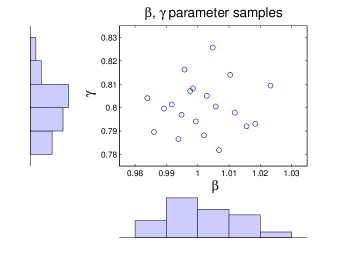
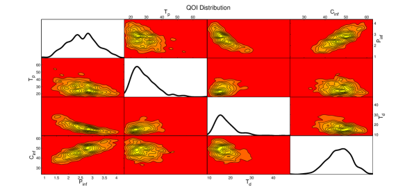
with $\mu_{\beta}=1$, $\sigma^{2}_{\beta}=0.000125$, $\mu_{\gamma}=0.8$, $\sigma^{2}_{\gamma}=0.000125$. These distributions and their corresponding univariate histograms of the samples are plotted in Figure 2. Besides uncertainty in the QOI caused by imprecisely known transmission and recovery rates, we must also account for the variation introduced by the stochasticity in the SIR model, an intrinsic uncertainty. When sampling $\vec{Q}(\beta,\gamma;\omega)$ to quantify the model’s uncertainty, we first draw $(\beta,\gamma)$ samples from the distributions in Equation (2.5). For each of these parameter sets, we then simulate multiple solutions to Equation (2.2) and record the samples of $\vec{Q}(\beta,\gamma;\omega)$. Repeating the simulation multiple times for each parameter set is essential to sample the contribution of intrinsic uncertainty to the distribution of the QOI. Once this is done, we use kernel density estimation [8] to form an approximate distribution of $\vec{Q}(\beta,\gamma;\omega)$. The result of this process is shown in Figure 3.

$\begin{array}[]{cc}\includegraphics[scale={0.3}]{SIRsde_infected_revised.pdf}&\includegraphics[scale={0.3}]{SIRsde_cuminfected_revised.pdf}\\ \end{array}$

Figure 1: A sample of $\vec{Q}(\beta,\gamma;\omega)$ from one SIR realization. (LEFT) % infected time series for a fixed $(\beta,\gamma)$. $Q_{1}$, $Q_{2}$, and $Q_{3}$ are labeled. (RIGHT) % cumulatively infected time series for a fixed $(\beta,\gamma)$, $Q_{4}$ is marked.

Figure 2: Samples of $(\beta,\gamma)$ parameters from their log-normal distributions and corresponding univariate histograms of the samples. These samples are then used as input parameters to (2.2), effectively exploring the contribution of parametric uncertainty to the distribution of $\vec{Q}(\beta,\gamma;\omega)$.

Figure 3: One dimensional and two dimensional marginal distributions from the four dimension distribution corresponding to $\vec{Q}(\beta,\gamma;\omega)$. Kernel density estimation was used to generate each of the marginal distributions from samples of the SIR model. The goal of the methods detailed in this paper is to be able to reconstruct an approximation of this distribution from very few samples of the actual SIR simulation and to be able to directly generate approximate samples of $\vec{Q}(\beta,\gamma;\omega)$ quickly.

Notation:

To ensure generality in our presentation and to avoid overly cumbersome notation, we denote $X(\theta;\omega)=(X_{\tau}(\theta;\omega))_{\tau=1}^{d}\in{\mathbb{R}}^{d}$ to represent our vector quantity of interest. Here, $\tau$ is a discrete index parameter indicating the specific QOI. In practice, $\tau$ could also represent discrete samples of a continuous parameter, e.g., time. The vector $\theta\in{\mathbb{R}}^{p}$ will denote input parameters to the simulation and $\omega$ is the state variable controlling stochastic variation.

For the simulation, output $X_{\tau}(\theta;\omega)$ uncertainty due to variation in $\theta$ will be parametric uncertainty. We will assume that we know the probability density for $\theta$ and can choose how we will sample from that density when the simulation is run. The uncertainty in our output due to $\omega$ will be referred to as intrinsic uncertainty, which is characterized by the absence of a parameterized probability space and by our inability to choose how to sample its effects.

For the SIR model, the notational translation will be $X_{\tau}(\theta;\omega)=Q_{\tau}(\beta,\gamma;\omega)$ with $\tau=1,2,3,4$ and $\theta=(\beta,\gamma)$.

3 Karhunen-Loeve decomposition

In this section, we use the Karhunen-Loeve (KL) decomposition to transform the QOI to a set of uncorrelated random variables. The lack of correlation between the transformed QOI will aid in our construction of a polynomial chaos representation of our model. Using the KL decomposition has the added benefit of possibly reducing the dimension of the QOI space being emulated.

We first decompose $X_{\tau}(\theta;\omega)$ so that the contributions from $\tau$ and $\theta$ are separated from those of $\omega$. Define

$$\overline{X}={\mathbb{E}}[X(\theta;\omega)]$$

so the process may be represented as

$$X(\theta;\omega)=\overline{X}+X^{0}(\theta;\omega).$$ (3.1)

The zero mean random vector $X^{0}(\theta;\omega)$ is now emulated.

In order to remove the correlations between the QOI and reduce dimensionality, we use a Karhunen-Loeve (KL) [10, 11] decomposition for $X^{0}$. The covariance function is given by the $d\times d$ square matrix

$$K(s,r)={\mathbb{E}}[X^{0}_{s}(\theta;\omega)X^{0}_{r}(\theta;\omega)],\,\,s,r=1,2,\dots,d.$$ (3.2)

In the KL decomposition, one then finds the eigenfunctions of the covariance by solving the eigenvalue problem

$$\sum_{r=1}^{d}K(\tau,r)f^{n}_{r}=\lambda_{n}f^{n}_{\tau},\,\,\tau,n=1,2,\dots,d.$$ (3.3)

The set of Euclidean unit length eigenvectors $\{f^{n}\}_{n=1}^{d}\subset\mathbb{R}^{d}$ forms a basis for the random vector $X^{0}(\theta;\omega)$ so we may project onto this basis. Coefficients of the projection are

$$\xi_{n}(\theta;\omega)=\langle X^{0}(\theta;\omega),f^{n}\rangle=\sum_{\tau=1}^{d}X^{0}_{\tau}(\theta;\omega)f^{n}_{\tau}.$$ (3.4)

The KL decomposition of the zero mean random vector is

$$X^{0}(\theta;\omega)=\sum_{n=1}^{d}\xi_{n}(\theta;\omega)f^{n}$$ (3.5)

and the truncated KL decomposition is obtained by taking the first $N<d$ terms in the series

$$X^{0}(\theta;\omega)\approx\sum_{n=1}^{N}\xi_{n}(\theta;\omega)f^{n}.$$ (3.6)

With Equation (3.6), we have reduced the emulation problem to the problem of emulating the random vector of uncorrelated coefficients $\xi(\theta;\omega)=(\xi_{1}(\theta;\omega),\dots,\xi_{N}(\theta;\omega))$. Since we are not assuming that $X(\theta;\omega)$ is Gaussian the coefficients, $\xi_{i}(\theta;\omega)$, are not necessarily Gaussian and therefore not necessarily independent.

Correlations between entries of $X(\theta;\omega)$, corresponding to different QOI, is now controlled by the entries of the eigenvectors $f^{n}$. If the eigenvalues in Equation (3.3) decay rapidly, the number of terms, $N$, can be taken to be much smaller than the original number of QOI, effectively reducing the output dimension.

Figure 4: Starting with the four dimensional distribution of $\vec{Q}(\beta,\gamma;\omega)$, shown in Figure 3, the KL decomposition is computed. In this figure, we show the one and two dimensional marginal distributions for the first three KL coefficients derived from the distribution of $\vec{Q}(\beta,\gamma;\omega)$. When compared to the marginal distributions in Figure 3, one can see that the correlations between the KL coefficients is less than those of the original QOI. This is important for implementation of the polynomial chaos decomposition.

Figure 5: The first three KL coefficients depicted in Figure 4 are used to reconstruct an approximation to the distribution of $\vec{Q}(\beta,\gamma;\omega)$. Using this approximation allows us to reduce the dimension of the QOI.

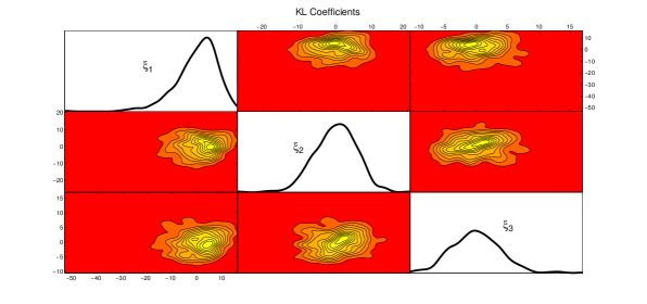
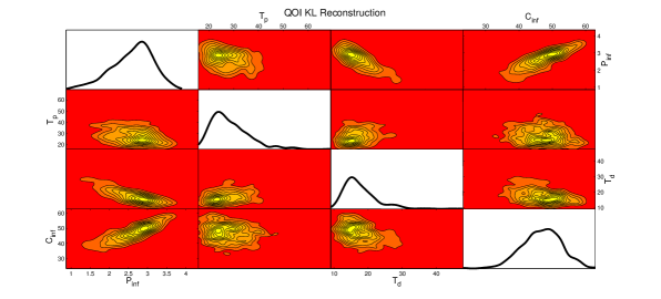
The effectiveness of the KL decomposition on our example problem is shown in Figures 4 and 5. Since our SIR model output, $\vec{Q}(\beta,\gamma;\omega)$, is only four dimensional, a complete KL decomposition has four coefficients. In Figure 4, the distribution of the first three KL coefficients is visualized. These coefficients are used to reconstruct an approximation to the distribution of $\vec{Q}(\beta,\gamma;\omega)$ shown in Figure 3. The approximate reconstruction has a distribution depicted in Figure 5.

4 Polynomial chaos expansion of coefficients

A reduced representation for the random vector of uncorrelated, but not independent, random variables $\xi(\theta;\omega)=(\xi_{1}(\theta;\omega),\dots,\xi_{N}(\theta;\omega))$ is constructed using a polynomial chaos (PC) decomposition. This accomplishes two goals. First, at a fixed $\theta$, the PC decomposition computes a low dimensional approximation to the distribution of $\xi(\theta;\omega)$ while still allowing for non-Gaussianity. Second, the PC approximation gives us a way to generate approximate samples from the distribution of $\xi(\theta;\omega)$ at a fixed parameterization $\theta$. Although KL gives a low dimensional approximation to the orginal distribution of $X(\theta;\omega)$ it does not provide a way to generate samples from that distribution.

In polynomial chaos, a random variable is approximated by a series of polynomial basis functions that form a basis for the underlying probability space of the random variable. It has been shown [22] that the particular choice of basis makes a significant difference in the rate of convergence to the random variable. We will present our methods using the Hermite polynomials [22], which work well for our SIR example, though the techniques used are independent of the basis. Different basis of polynomials, in the generalized polynomial chaos scheme, are orthogonal with respect to different measures. The Hermite polynomials are orthogonal with respect to the standard Gaussian density. This makes them ideal for application when the underlying distribution of the random variable being emulated is approximately normal. If there is reason to suspect that a distribution is far from normal then another basis should be considered [22].

The Hermite polynomial of degree $k$ in a single dimension is denoted by $\psi_{k}(x)$. This set of polynomials can be defined recursively by

$$\psi_{0}(x) =1$$ (4.1)

$$\psi_{1}(x) =x$$

$$\psi_{m+1}(x) =x\psi_{m}(x)-m\psi_{m-1}(x)\textrm{ for }m=1,2,\dots.$$

Since the Hermite polynomials are orthogonal with respect to the standard normal density

$$w(x)\,dx=\frac{1}{\sqrt{2\pi}}e^{-x^{2}/2}\,dx,$$

the relation

$$\frac{1}{\sqrt{2\pi}}\int_{-\infty}^{\infty}\psi_{i}(x)\psi_{j}(x)e^{-x^{2}/2}\,dx=j!\delta_{ij}$$

holds for all $i,j=0,1,2,\dots$. The Hermite polynomials in higher dimensions are formed by tensor product. Let $\alpha=(\alpha_{1},\alpha_{2},\dots,\alpha_{d})\in{\mathbb{Z}}^{d}$ be a multi-index and define the Hermite polynomial on ${\mathbb{R}}^{d}$ by

$$\Psi_{\alpha}({\bf x})=\psi_{\alpha_{1}}(x_{1})\psi_{\alpha_{2}}(x_{2})\dots\psi_{\alpha_{d}}(x_{d}).$$ (4.2)

To index the Hermite polynomials in higher dimensions, we use a graded lexicographic ordering [4] on the multi-indices in dimension $d$. That is, we will use $\Psi_{k}({\bf x})$ to refer to the multidimensional Hermite polynomial with the $k^{th}$ multi-index in the graded lexicographic ordering.

With the above indexing on higher dimensional Hermite polynomials, the polynomial chaos decomposition of the random vector $\xi(\theta;\omega)$, up to order $K$, is given by

$$\xi(\theta)=\xi(\theta;\omega(\zeta))\approx\sum_{k=0}^{K}{\bf c}_{k}(\theta)\Psi_{k}(\zeta).$$ (4.3)

Here ${\bf c}_{k}(\theta)$ is a length $N$ vector of coefficients corresponding to each entry in $\xi$ so, for $n=1,2,\dots,N$,

$$\xi_{n}(\theta)=\xi_{n}(\theta;\omega(\zeta))\approx\sum_{k=0}^{K}c_{nk}(\theta)\Psi_{k}(\zeta).$$ (4.4)

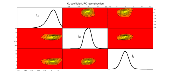
The new variable $\zeta=(\zeta_{1},\zeta_{2},\dots,\zeta_{N})$ is a random vector of independent standard normal random variables. This vector serves the purpose of parameterizing the probability space corresponding to $\omega$. That is, sampling from $\zeta$ is equivalent to sampling from $\omega$. In Figure 6, we show the reconstruction of the first three KL coefficients for the QOI in the stochastic SIR model using Equation (4.4).

Figure 6: Reconstruction of the one and two dimensional marginal distributions for KL coefficients using the first eight terms in the polynomial chaos reconstruction given by Equations (4.3)–(4.4). Since the Hermite polynomial chaos approximation is formed from smooth functions sampling from the truncated decomposition has the effect of smoothing the original distribution and clipping the low probability regions. This can be observed by comparing the above Figure with the original KL distribution in Figure 4.

The difficulty with the expansion given by Equations (4.3)–(4.4) is the computation of the coefficients ${\bf c}_{k}(\theta)$. These are formally defined through Galerkin projection onto the Hermite polynomials [22] by the formula

$$c_{nk}(\theta)=\frac{{\mathbb{E}}[\xi_{n}(\theta;\omega)\Psi_{k}(\zeta)]}{{\mathbb{E}}[\Psi_{k}^{2}(\zeta)]}.$$ (4.5)

This formula is only formal since $\xi_{n}(\theta;\omega)$ and $\Psi_{k}(\zeta)$ live over different probability spaces. Computing the expectation ${\mathbb{E}}[\xi_{n}(\theta;\omega)\Psi_{k}(\zeta)]$ in Equation (4.5) is performed by Monte Carlo approximation, so sampling of $\xi_{n}(\theta;\omega)$ and $\Psi_{k}(\zeta)$ must take place over the same probability space. To compute this expectation, we transform the two probability spaces to a common domain. There is a standard method to transform two different, finite dimensional, probability spaces into a common space, which usually relies on having an explicit representation of the underlying distributions. Lacking an explicit representation, we will form an approximation using a kernel density estimate.

The Rosenblatt transformation [19] uses the conditional cumulative distribution functions to map a set of jointly distributed random variables onto a set of independent uniform random variables on $[0,1]$. In terms of the conditional cumulative distribution, the Rosenblatt transformation is given by

$$u_{1} =F_{1}(\xi_{1})$$ (4.6)

$$u_{2} =F_{2|1}(\xi_{2}|\xi_{1})$$

$$u_{3} =F_{3|1,2}(\xi_{3}|\xi_{1},\xi_{2})$$

$$\vdots$$

$$u_{N} =F_{N|1,2,\dots,N-1}(\xi_{N}|\xi_{1},\xi_{2},\dots,\xi_{N}).$$

Once this map is computed, the cumulative distributions are used to generate samples from the joint distribution of the random vector $\xi$ from $N$ independent samples of uniform random variables on $[0,1]$. This process is the inverse Rosenblatt transformation, which maps a set of $N$ independent uniformly distributed random variables to the random vector $\xi$ of length $N$. This process uses the inverses of each of the marginal cumulative distributions in Equation (4.6). We will denote this inverse Rosenblatt transform by

$$g({\bf u})=\xi,{\bf u}\sim U[0,1]^{N}.$$ (4.7)

Likewise it is standard to map ${\bf u}\sim U[0,1]^{N}$ to independent normally distributed random variables $\zeta\sim N(0,1)^{N}$. We denote this map by

$$l({\bf u})=\zeta,{\bf u}\sim U[0,1]^{N}.$$ (4.8)

With the above maps one can then compute the expectation in the numerator of (4.5) as follows,

$${\mathbb{E}}[\xi_{n}(\theta;\omega)\Psi_{k}(\zeta)] =\frac{1}{(2\pi)^{N/2}}\int\xi_{n}(\theta;\omega)\Psi_{k}(\zeta)e^{-\frac{1}{2}{|\!|}\zeta{|\!|}^{2}}\,d\zeta$$ (4.9)

$$=\int_{[0,1]^{N}}g_{\theta}({\bf u})\Psi_{k}(l({\bf u}))\,d{\bf u}.$$

We note that the integral is computed using a Monte Carlo approach and we have used the notation $g_{\theta}({\bf u})$ to indicate that the particular inverse Rosenblatt transformation depends on the parameter $\theta$. As stated above, to calculate the expectation in Equation (4.9) using a Monte Carlo scheme one must be sure to use the same sample of the uniform random variable ${\bf u}$ when calculating values for $g_{\theta}({\bf u})$ and $l({\bf u})$. It is also important to use a Monte Carlo scheme of sufficient order relative to the size of the coefficients involved in Equation (4.3).

When using Equation (4.3) to characterize intrinsic uncertainty in a simulation, one does not have an explicit form for the conditional cumulative functions in (4.6). In practice, for a fixed $\theta$, one only has a finite number of samples of the random vector $\xi(\theta;\omega)$, which we will denote by $\{\xi^{(m)}\}_{m=1}^{M}$. To estimate the conditional cumulative functions, we first use the samples to estimate the joint pdf of the random vector $\xi$. This can be done using a kernel density estimation (KDE) method [8]. We use univariate tensor product kernels where our univariate kernel for the $i^{th}$ variable is denoted by $K_{i}(\xi_{i})$ and our bandwidth is denoted by $h>0$. For the derivations that follow, it is important to recall that, in KDE, the kernel $K_{i}$ has integral equal to one. For the samples $\{\xi^{(m)}\}_{m=1}^{M}\subset{\mathbb{R}}^{d}$ the KDE at a point $\xi=(\xi_{1},\xi_{2},\dots,\xi_{d})$ is given by

$$p(\xi) =\frac{1}{Mh^{d}}\sum_{m=1}^{M}\mathcal{K}\left(\frac{\xi-\xi^{(m)}}{h}\right)$$ (4.10)

$$=\frac{1}{Mh^{d}}\sum_{m=1}^{M}K_{1}\left(\frac{\xi_{1}-\xi^{(m)}_{1}}{h}\right)K_{2}\left(\frac{\xi_{2}-\xi^{(m)}_{2}}{h}\right)\cdots K_{d}\left(\frac{\xi_{d}-\xi^{(m)}_{d}}{h}\right).$$

The goal is to now use Equation (4.10) to build the conditional cumulative distributions in the functions (4.6). The cumulative distribution functions are built from the marginal densities,

$$p_{1,\dots,n}(\xi_{1},\dots,\xi_{n}) =\int p(\xi)\,d\xi_{n+1}\cdots d\xi_{d}$$ (4.11)

$$=\frac{1}{Mh^{n}}\sum_{m=1}^{M}K_{1}\left(\frac{\xi_{1}-\xi^{(m)}_{1}}{h}\right)\cdots K_{n}\left(\frac{\xi_{n}-\xi^{(m)}_{n}}{h}\right).$$

This leads directly to a formula for the marginal conditional cumulative distributions

$$F_{n|n-1,\dots,1}(\xi_{n}|\xi_{1},\dots,\xi_{n-1}) =\int_{-\infty}^{\xi_{n}}p_{n|n-1,\dots,1}(\tilde{\xi}_{n}|\xi_{1},\dots,\xi_{n-1})\,d\tilde{\xi}_{n}$$ (4.12)

$$=\int_{-\infty}^{\xi_{n}}\frac{p_{1,\dots,n}(\xi_{1},\dots,\tilde{\xi}_{n})}{p_{1,\dots,n-1}(\xi_{1},\dots,\xi_{n-1})}\,d\tilde{\xi}_{n}$$

$$=\frac{\sum_{m=1}^{M}\left[\left\{\prod_{l=1}^{n-1}K_{l}\left(\frac{\xi_{l}-\xi_{l}^{(m)}}{h}\right)\right\}\frac{1}{h}\int_{-\infty}^{\xi_{n}}K_{n}\left(\frac{\tilde{\xi}_{n}-\xi_{n}^{(m)}}{h}\right)\,d\tilde{\xi}_{n}\right]}{\sum_{m=1}^{M}\left\{\prod_{l=1}^{n-1}K_{l}\left(\frac{\xi_{l}-\xi_{l}^{(m)}}{h}\right)\right\}}.$$

Once these can be computed, the inverse Rosenblatt transform is easily accomplished. For each sample ${\bf u}\sim U[0,1]^{d}$, one iteratively goes through the dimensions starting by computing $F_{1}(\xi_{1})$ for increasing $\xi_{1}$ until $F_{1}(\xi_{1})\geq u_{1}$, which fixes a $\xi_{1}$. Next compute $F_{2|1}(\xi_{2}|\xi_{1})$ for increasing $\xi_{2}$ until $F_{2|1}(\xi_{2}|\xi_{1})\geq u_{2}$, which fixes $\xi_{2}$. This process is repeated $d$ times until we arrive at a map $g({\bf u})=\xi$.

Now that we have a method of computing the expectations in the polynomial chaos coefficient definitions (4.5), it is possible for us to build an emulator from our data that combine the Karhunen-Loeve decomposition in Equation (3.6) and the polynomial chaos expansion in Equation (4.3). This gives us an approximate model for the stochastic process represented in the simulation,

$$X(\theta;\omega(\zeta))\approx\overline{X}+\sum_{n=1}^{N}\left(\sum_{k=1}^{K}c_{nk}(\theta)\Psi_{k}(\zeta)\right)f^{n}.$$ (4.13)

The PC expansion must be computed separately for each value of our input parameter set, $\theta$. The dependence of the stochastic process on the input variables is then only seen through the coefficients $c_{nk}(\theta)$ in the PC expansion. One important property of this emulation is to provide a map from the multivariate standard normal random variable $\zeta$ to the intrinsic uncertainty in the random vector $\xi(\theta;\omega)$. This defines a probability space for the intrinsic uncertainty in the simulation that can be sampled quickly. Once the emulator is constructed, for a fixed set of inputs, many realizations may be computed to ascertain the approximate distributions associated with quantities of interest when only intrinsic uncertainty is present. The use of the polynomial chaos decomposition allows this intrinsic uncertainty to be represented in a non-Gaussian, and somewhat, non-parametric way which has the potential to represent very general behavior in the intrinsic variability.

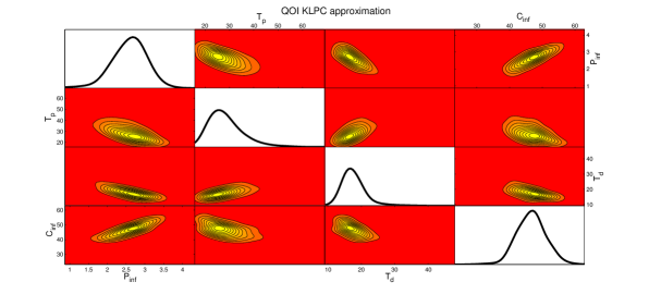
An approximation of Equation (4.13) is depicted, for the SIR example, in Figure 7. Again, we see the smoothing out of the QOI distribution’s finer scale features. However, general shape, correlation structure, and non-Gaussianity are preserved well. This approximation can be made exact by increasing the number of samples from the SIR model used to form the KL decomposition and the PC decomposition as well as including more terms in each of the decompositions.

Figure 7: Reconstruction of the one and two dimensional marginal distributions of the QOI using the KL-PC decomposition in (4.13). This figure should be compared with the original QOI distribution depicted in Figure 3. Notice that much of the original distribution structure is maintained. However, the approximation inevitably smooths the original distribution and cuts off some of the lower probability regions. This is due to a mixture of the effects of truncation in the KL-PC decomposition and the bandwidth chosen in the KDE used to compute the PC coefficients.

5 Gaussian process regression on PC coefficients

It remains to provide a surrogate model for the dependence of the stochastic process on the parameterization, $\theta$. From the KL-PC approximation in (4.13) for each set of inputs, we arrive at a set of $N\!\!\cdot\!K$ coefficients $c_{nk}(\theta)$. We perform Gaussian process (GP) regression on the coefficients with the samples from sets of input parameters as data. There are many good reviews on the advantages of Gaussian processes in statistical modeling [12, 14]. We highlight two properties that are particularly important. First, a Gaussian process regression is an interpolant. If the coefficients are computed at a specific $\theta$ value and a Gaussian process is formed for the coefficients, then the GP coefficient values will equal the observed coefficients at that $\theta$ value. Second, a Gaussian process regression fits a process to data through a series of observed input values, which is done in a way that ensures the variance in the process will grow for $\theta$ values that are farther away from observations. This allows uncertainty in the emulator to emerge that is attributable to lack of observations, realizations taken at too few sets of input parameters, and to describe the actual dependencies of the simulation on input parameters.

To build the GP regression, we follow the methods introduced in [7, 21], the necessary details are included for completeness. First, we form a vector of the coefficients,

$$\vec{c}(\theta)=(c_{11}(\theta),c_{12}(\theta),\dots,c_{21}(\theta),c_{22}(\theta),\dots,c_{N(K-1)}(\theta),c_{NK}(\theta))^{T}.$$ (5.1)

The statistical surrogate model is then built for $\vec{c}:{\mathbb{R}}^{p}\rightarrow{\mathbb{R}}^{N\cdot K}$. If the PC coefficients are constructed (i.e., sampled) at $m$ parametric values $\{\theta_{1},\theta_{2},\dots,\theta_{m}\}$, then we can form the $(NK)\times m$ data matrix,

$${\mathcal{C}}=\left(\begin{array}[]{cccc}c_{11}(\theta_{1})&c_{11}(\theta_{2})&\dots&c_{11}(\theta_{m})\\ c_{12}(\theta_{1})&c_{12}(\theta_{2})&\dots&c_{12}(\theta_{m})\\ \vdots&\vdots&\ddots&\vdots\\ c_{NK}(\theta_{1})&c_{NK}(\theta_{2})&\dots&c_{NK}(\theta_{m})\end{array}\right).$$ (5.2)

This is then standardized by subtracting the mean over all the samples and dividing by the standard deviation of all the coefficients to form ${\mathcal{C}}_{\textrm{std}}$. This standardized data matrix is then decomposed using a singular value decomposition. In addition, a truncated $(NK)\times p_{c}$ matrix of singular vectors is constructed, $K=[{\bf k}_{1},{\bf k}_{2},\dots,{\bf k}_{p_{c}}]$ with ${\bf k}_{i}\in{\mathbb{R}}^{N\cdot K}$. We truncate the singular vectors to keep only those corresponding to large singular values. ${\mathcal{C}}_{\textrm{std}}$ is used to build an emulator, corresponding to a standardized map $\vec{c}_{\textrm{std}}:{\mathbb{R}}^{p}\rightarrow{\mathbb{R}}^{N\cdot K}$, of the form

$$\vec{c}_{\textrm{std}}(\theta) \approx\sum_{i=1}^{p_{c}}{\bf k}_{i}w_{i}(\theta;\eta)+\delta(\eta)$$ (5.3)

$$=KW(\theta;\eta)+\delta(\eta)$$

where $W(\theta;\eta)=(w_{1}(\theta;\eta),\dots,w_{p_{c}}(\theta;\eta))^{T}$ and $\delta(\eta)$ is an independent zero mean Gaussian process modeling the discrepancy between the truncated decomposition and the data. This is taken to be $\delta(\eta)\sim{\mathcal{N}}({\bf 0}_{NK},\lambda_{\delta}^{-1}I_{NK})$ with hyperparameter $\lambda_{\delta}$. The parameter $\lambda_{\delta}$ will control how much noise is present, we will refer to $\lambda_{\delta}$ as the noise precision parameter. Here $w_{i}(\theta;\eta)$ will be $p_{c}$ independent zero mean Gaussian processes over the input space $\theta\in{\mathbb{R}}^{p}$. These will be constructed from the $p_{c}\times m$ matrix

$$\mathcal{W}=\left(\begin{array}[]{cccc}w_{1}(\theta_{1})&w_{1}(\theta_{2})&\dots&w_{1}(\theta_{m})\\ w_{2}(\theta_{1})&w_{2}(\theta_{2})&\dots&w_{2}(\theta_{m})\\ \vdots&\vdots&\ddots&\vdots\\ w_{p_{c}}(\theta_{1})&w_{p_{c}}(\theta_{2})&\dots&w_{p_{c}}(\theta_{m})\end{array}\right)$$ (5.4)

coming from the truncated singular value decomposition, ${\mathcal{C}}_{\textrm{std}}=K\mathcal{W}$.

Each of the $w_{i}(\theta;\eta)$ have covariance model [7]

$$R(\theta,\theta^{\prime})=\frac{1}{\lambda_{w_{i}}}\prod_{k=1}^{p}\rho_{w_{i}(k)}^{4(\theta_{(k)}-\theta^{\prime}_{(k)})^{2}}$$ (5.5)

with hyperparameters $\lambda_{w_{i}}$ and $\vec{\rho}_{w_{i}}=(\rho_{w_{i}(1)},\dots,\rho_{w_{i}(p)})^{T}$. We will choose prior distributions on the hyperparameters that ensure $\rho_{w_{i}(k)}\in(0,1)$ so that $R(\theta,\theta^{\prime})$ decays as ${|\!|}\theta-\theta^{\prime}{|\!|}\rightarrow\infty$. The notation $\theta_{(k)}$ is used to denote the $k^{th}$ coordinate of $\theta\in{\mathbb{R}}^{p}$. For the Bayesian regression, we define the length $m$ vector ${\bf w}_{i}=(w_{i}(\theta_{1}),w_{i}(\theta_{2}),\dots,w_{i}(\theta_{m}))^{T}$ for $i=1,2,\dots,p_{c}$. The vector ${\bf w}_{i}$ has covariance given by

$$\lambda_{w_{i}}^{-1}C(\theta;\vec{\rho}_{w_{i}}).$$ (5.6)

A symmetric $m\times m$ matrix is obtained by applying the covariance model (5.5) to each pair in the sample set $\{\theta_{1},\dots,\theta_{m}\}$.

Now we define the $mp_{c}$ vector of all processes ${\bf w}_{i}$ evaluated at the sample points, $\vec{{\bf w}}=({\bf w}_{1}^{T},{\bf w}_{2}^{T},\dots,{\bf w}_{p_{c}}^{T})^{T}$, distributed as

$$\vec{{\bf w}} \sim{\mathcal{N}}({\bf 0}_{mp_{c}},\Sigma_{{\bf w}}+\lambda_{\delta}^{-1}I_{mp_{c}})$$ (5.7)

$$\Sigma_{{\bf w}} =\operatornamewithlimits{diag}_{i=1,\dots,p_{c}}(\lambda_{w_{i}}^{-1}C(\theta;\vec{\rho}_{w_{i}})),$$ (5.8)

the covariance matrix being size $(mp_{c})\times(mp_{c})$.

Then the $m\cdot(NK)$ column vector of the standardized data

$$\vec{{\bf c}}_{\textrm{std}}=(\vec{c}_{\textrm{std}}(\theta_{1})^{T},\vec{c}_{\textrm{std}}(\theta_{2})^{T},\dots,\vec{c}_{\textrm{std}}(\theta_{m})^{T})^{T}$$

is distributed

$$\vec{{\bf c}}_{\textrm{std}}\sim{\mathcal{N}}({\bf 0}_{m\cdot(NK)},\tilde{K}\Sigma_{{\bf w}}\tilde{K}^{T}+\lambda_{\delta}^{-1}I_{m\cdot(NK)}).$$ (5.9)

Where $\tilde{K}=[I_{m}\otimes{\bf k}_{1},I_{m}\otimes{\bf k}_{2},\dots,I_{m}\otimes{\bf k}_{p_{c}}]$ is the $(m\cdot(NK))\times(mp_{c})$ matrix formed by the Kronecker product of the principle vectors. Notice that from Equation (5.3), it follows that $\tilde{K}^{T}\vec{{\bf c}}_{\textrm{std}}=\vec{{\bf w}}$.

Relations (5.3) and (5.7)-(5.9) define a likelihood coming from the density of the normal distribution

$$L(\vec{{\bf w}}|\lambda_{\delta},\lambda_{w_{i}},\vec{\rho}_{w_{i}},i=1,\dots,p_{c}).$$ (5.10)

In the regression step the posterior distribution is given by

$$p(\lambda_{\delta},\lambda_{w_{i}},\vec{\rho}_{w_{i}},i=1,\dots,p_{c}|\vec{{\bf w}}) \propto$$ (5.11)

$$L(\vec{{\bf w}}|\lambda_{\delta},\lambda_{w_{i}},\vec{\rho}_{w_{i}},i=1,\dots,p_{c})\pi(\lambda_{\delta})\prod_{i=1}^{p_{c}}\left\{\pi(\lambda_{w_{i}})\prod_{k=1}^{p}\pi(\rho_{w_{i}(k)})\right\}.$$

This is sampled using a Metropolis-Hastings MCMC [18] method such as a univariate random walk or an independence sampler. One can either take the estimated maximum likelihood values for the hyperparameters $\lambda_{\delta}$, $\lambda_{w_{i}}$, $\vec{\rho}_{w_{i}}$ or choose a range of values from the samples.

We assume the $\lambda$ hyperparameters have prior gamma distributions and the $\rho$ hyperparameters have beta distribution priors [7],

$$\pi(\lambda_{w_{i}}) \propto\lambda_{w_{i}}^{a_{w}-1}e^{-b_{w}\lambda_{w_{i}}},\,i=1,2,\dots,p_{c}$$ (5.12)

$$\pi(\rho_{w_{i}(k)}) \propto\rho_{w_{i}(k)}^{a_{\rho}-1}(1-\rho_{w_{i}(k)})^{b_{\rho}-1},\,i=1,2,\dots,p_{c},\,k=1,2,\dots,p$$

$$\pi(\lambda_{\delta}) \propto\lambda_{\delta}^{a_{\delta}-1}e^{-b_{\delta}\lambda_{\delta}}.$$

Once values of the hyperparameters are chosen through exploration of the posterior (5.11), predictions can be made for the emulated $\vec{c}_{\textrm{std}}(\theta^{*})$ at some new parameter set $\theta^{*}\in{\mathbb{R}}^{p}$. Let the prediction vector, at a set of parameter values $\{\theta^{*}_{1},\theta^{*}_{2},\dots,\theta^{*}_{s}\}$, be denoted $\vec{{\bf c}}^{*}_{\textrm{std}}=(\vec{c}_{\textrm{std}}(\theta^{*}_{1})^{T},\vec{c}_{\textrm{std}}(\theta^{*}_{2})^{T},\dots,\vec{c}_{\textrm{std}}(\theta^{*}_{s})^{T})^{T}$, a length $s\cdot(NK)$ column vector. The prediction is based on prediction of the $s\cdot p_{c}$ vector $\vec{{\bf w}}^{*}=(({\bf w}^{*}_{1})^{T},({\bf w}^{*}_{2})^{T},\dots,({\bf w}^{*}_{p_{c}})^{T})^{T}$, where ${\bf w}^{*}_{i}=(w_{i}(\theta^{*}_{1}),w_{i}(\theta^{*}_{2}),\dots,w_{i}(\theta^{*}_{s}))^{T}$ for $i=1,2,\dots,p_{c}$.

From our definitions above we see that the data vector and prediction vector are jointly distributed as

$$\left[\begin{array}[]{c}\vec{{\bf w}}\\ \vec{{\bf w}}^{*}\end{array}\right]\sim{\mathcal{N}}(0_{(s+m)p_{c}},\Xi+\lambda_{\delta}^{-1}I_{(s+m)p_{c}}),\,\Xi=\left[\begin{array}[]{cc}\Sigma_{{\bf w}}&\Sigma_{{\bf ww^{*}}}\\ \Sigma_{{\bf w^{*}w}}&\Sigma_{{\bf w^{*}}}\end{array}\right].$$ (5.13)

The terms in the covariance matrix come from applying our covariance model (5.5) to each pair of the respective parameter sets. Thus, $\Sigma_{{\bf w}}$ is the $m\cdot p_{c}$ square matrix obtained by applying Equation (5.5) to each pair in the sample set $\{\theta_{1},\dots,\theta_{m}\}$ for each ${\bf w}_{i}$. Similarly, $\Sigma_{{\bf w^{*}}}$ is the $s\cdot p_{c}$ square matrix obtained by applying Equation (5.5) to each pair in the prediction set $\{\theta^{*}_{1},\dots,\theta^{*}_{s}\}$ for each ${\bf w}^{*}_{i}$. Finally, $\Sigma^{T}_{{\bf ww^{*}}}=\Sigma_{{\bf w^{*}w}}$ is the $(s\cdot p_{c})\times(m\cdot p_{c})$ matrix obtained by applying Equation (5.5) to each pair $(\theta_{k},\theta^{*}_{j})$ in the sample and prediction set. The predictions are then distributed as follows:

$$\vec{{\bf w}}^{*} \sim{\mathcal{N}}(\mu^{*},\Omega^{*})$$ (5.14)

$$\mu^{*} =\Sigma_{{\bf w^{*}w}}\left(\Sigma_{{\bf w}}+\lambda_{\delta}^{-1}I_{mp_{c}}\right)^{-1}\vec{{\bf w}}$$

$$\Omega^{*} =\left(\Sigma_{{\bf w^{*}}}+\lambda_{\delta}^{-1}I_{sp_{c}}\right)-\Sigma_{{\bf w^{*}w}}\left(\Sigma_{{\bf w}}+\lambda_{\delta}^{-1}I_{mp_{c}}\right)^{-1}\Sigma_{{\bf ww^{*}}}.$$

From the predictions $\vec{{\bf w}}^{*}$, we can define predicted standardized polynomial chaos coefficients using the relations

$$\vec{{\bf c}}^{*}_{\textrm{std}} =\tilde{K}^{*}\vec{{\bf w}}^{*}$$ (5.15)

$$\tilde{K}^{*} =[I_{s}\otimes{\bf k}_{1},I_{s}\otimes{\bf k}_{2},\dots,I_{s}\otimes{\bf k}_{p_{c}}].$$ (5.16)

Thus, after destandardization, we have defined a new map through Bayesian Gaussian process regression for the coefficients denoted by

$$\tilde{c}(\theta;\eta)=(\tilde{c}_{11}(\theta;\eta),\tilde{c}_{12}(\theta;\eta),\dots,\tilde{c}_{21}(\theta;\eta),\dots,\tilde{c}_{NK}(\theta;\eta))^{T}.$$ (5.17)

The random variable $\eta$ is the associated state space variable for the Gaussian process. For a given realization of the GP regression $\eta$ is fixed.

Once the GP is formed for the PC coefficients, we build a complete emulator of the intrinsic and parametric uncertainty in the simulation. The final form of the statistical surrogate is

$$\mathcal{X}^{e}(\theta;\zeta,\eta)=\overline{X}+\sum_{n=1}^{N}\left(\sum_{k=1}^{K}\tilde{c}_{nk}(\theta,\eta)\Psi_{k}(\zeta)\right)f^{n}.$$ (5.18)

Figure 8: One and two dimensional marginal distributions of the KL coefficients for the SIR QOI. These were reconstructed using Gaussian process regression on the polynomial chaos coefficients depicted in Figure 6 using equation (5.18).

Figure 9: One and two dimensional marginal distributions of the SIR QOI reconstructed using our combination of Karhunen-Loeve, polynomial chaos, and Gaussian process regression. This is an approximation of the original distribution in Figure 3. The approximation captures the overall shape and range of the original QOI. However, the approximation does concentrate more around the mode of the original distribution. As sample size increases this effect will diminish.

In Equation (5.18), the contributions from each of the separate sources of uncertainty is represented explicitly. The first source of variation is the change between QOI. This variation is controlled in the emulator through the KL decomposition parameter $\tau$. Intrinsic variation is represented in $\mathcal{X}^{e}$ by the standard multivariate normal random variable $\zeta$ arising from the PC expansion. The parameter $\theta$ occurs in the GP of the coefficients and controls the dependence of the emulator on the input parameters. Lastly, the use of a GP regression to relate PC coefficients at distinct $\theta$ values introduces a new source of uncertainty that is not originally present in the model. This is uncertainty in the emulator’s dependence on the inputs that has arisen from lack of sampling in $\theta$. The random variable $\eta$ now quantifies this uncertainty, giving a way to sample from the emulator that will inform how effective the input evaluation scheme was.

In using $\mathcal{X}^{e}$ to compute approximate probabilities of specific outcomes from the simulation, each of these variables can be sampled independently. This permits independent study of each source of variation in the model to quantify its effects on the simulation predictions. Moreover, it allows one to study regions of the input space where surrogate model discrepancy is largest, i.e., where $\eta$ has the biggest contribution. This provides a framework to determine what simulation realizations would improve $\mathcal{X}^{e}$ the most.

We use samples of $\vec{Q}$ to compute a statistical emulator for the stochastic SIR model. We denote the emulation by

$$\vec{Q}_{e}(\beta,\gamma;\eta,\zeta) ={\mathbb{E}}[\vec{Q}]+\sum_{n=1}^{4}\left(\sum_{k=1}^{K}\tilde{c}_{nk}(\beta,\gamma;\eta)\Psi_{k}(\zeta)\right)\vec{f}_{n}$$ (5.19)

$$\beta\sim\ln{\mathcal{N}}(\mu_{\beta},\sigma^{2}_{\beta}), \,\,\gamma\sim\ln{\mathcal{N}}(\mu_{\gamma},\sigma^{2}_{\gamma}),\,\,\zeta\sim{\mathcal{N}}(0_{4},I_{4}).$$ (5.20)

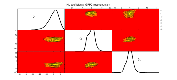
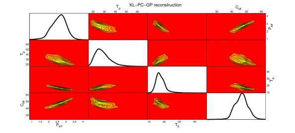
The reconstruction of the first three KL coefficients using Gaussian process emulation of the PC coefficients in our KL decomposition is shown in Figure 8. Then the KL reconstruction can be used to approximate the original QOI random variable. The distribution of this approximating random variable is depicted in Figure 9. Overall the shape of the distribution is maintained but more importantly, by using this approximation, we have the ability to sample from each source of uncertainty separately.

Recall, $\eta$ represents the state variable of the Gaussian process $\tilde{c}_{nk}$. The variables $(\beta,\gamma)$ can be sampled to explore the uncertainty in $\vec{Q}_{e}$ due to uncertainty in the input parameters. Similarly, $\zeta$ can be sampled to explore the uncertainty contribution due to intrinsic variation in the model. Finally, we can take many realizations of the Gaussian process $\tilde{c}_{nk}$ to study the uncertainty in the emulator $\vec{Q}_{e}$ introduced by lack of sampling of the actual simulation $\vec{Q}$.

Since realizations of the emulator $\vec{Q}_{e}$ are fast, we can use a Monte Carlo method combined with KDE to reconstruct an approximation of the distribution of $\vec{Q}$. This distribution can then be used to estimate probabilities of events associated with the quantities of interest in $\vec{Q}$.

6 Conclusion

We have discussed the problem of propagating uncertainty through a simulation that yields predictions effected by both intrinsic and parametric uncertainty. The term parametric uncertainty was used to characterize sources of variation in the simulation’s predictions for which the researcher knows the associated probability space and has control of how it is sampled when running the simulation. Intrinsic uncertainty was defined as variation in the simulation’s predictions that lacked an underlying parameterized probability space and/or a source of variation the researcher did not have control over.

The statistical emulator constructed yielded a parametrization of the intrinsic probability space that allowed for non-Gaussianity and separated the different sources of uncertainty in the output. This approach included accounting for uncertainty introduced from lack of sampling the simulation.

We used a stochastic system of ordinary differential equations, representing a simple disease model, to illustrate our methods. We allowed the input parameters of infection rate and recovery rate to be random variables with lognormal distributions. The four quantities of interest, the peak infected percent of the population, the time to the peak of the epidemic, the duration of the outbreak, and the total percent of the population infected, were then emulated from samples.

The emulation methods have potential application to uncertainty quantification in large scale computer simulations. Their utility can be evaluated by their ability to reconstruct joint distributions of QOI accurately from samples of the simulation. However, the emulation method has a large variety of tuning parameters and therefore requires human supervision in its application. It would, therefore, be of great utility to have reliable heuristics and theorems that give precise hypotheses on the types of stochastic processes for which the emulator will converge and the emulator’s rate of convergence, based on sampling size of the simulation. This is especially true in the case of stochastic processes whose distribution at a given parameter set depend on the parameter values. In the absence of theorems on convergence and rates of convergence for statistical surrogates, one would like to have a good suite of numerical tools at their disposal to evaluate the performance of the emulator. Such methods would need to be non-parametric and non-intrusive to be able to be applied to a large range of simulations without a priori assumptions. In the future, we will pursue these types of convergence results and numerical evaluation methods.

References

- [1] L. Allen. An introduction to stochastic epidemic models. Mathematical Epidemiology, pages 81–130, 2008.
- [2] L. Allen, A.M. Burgin, et al. Comparison of deterministic and stochastic SIS and SIR models in discrete time. Mathematical Biosciences, 163(1):1–34, 2000.
- [3] Roy M Anderson and Robert McCredie May. Infectious diseases of humans, volume 1. Oxford university press Oxford, 1991.
- [4] D.A. Cox, J. Little, and D. O’Shea. Ideals, varieties, and algorithms: an introduction to computational algebraic geometry and commutative algebra, volume 10. Springer, 2007.
- [5] John J Grefenstette, Shawn T Brown, Roni Rosenfeld, Jay DePasse, Nathan TB Stone, Phillip C Cooley, William D Wheaton, Alona Fyshe, David D Galloway, Anuroop Sriram, et al. Fred (a framework for reconstructing epidemic dynamics): an open-source software system for modeling infectious diseases and control strategies using census-based populations. BMC public health, 13(1):940, 2013.
- [6] J.C. Helton, J.D. Johnson, W.L. Oberkampf, and C.J. Sallaberry. Representation of analysis results involving aleatory and epistemic uncertainty. International Journal of General Systems, 39(6):605–646, 2010.
- [7] D. Higdon, J. Gattiker, B. Williams, and M. Rightley. Computer model calibration using high-dimensional output. Journal of the American Statistical Association, 103(482):570–583, 2008.
- [8] A.J. Izenman. Recent developments in nonparametric density estimation. Journal of the American Statistical Association, 86(413):205–224, 1991.
- [9] Ioannis Karatzas. Brownian motion and stochastic calculus, volume 113. springer, 1991.
- [10] Kari Karhunen. Über lineare Methoden in der Wahrscheinlichkeitsrechnung, volume 37. Universitat Helsinki, 1947.
- [11] Michel Loeve. Probability theory, vol. ii. Graduate texts in mathematics, 46:0–387, 1978.
- [12] D.J.C. MacKay. Introduction to gaussian processes. NATO ASI Series F Computer and Systems Sciences, 168:133–166, 1998.
- [13] Susan M Mniszewski, Sara Y Del Valle, Phillip D Stroud, Jane M Riese, and Stephen J Sydoriak. Episims simulation of a multi-component strategy for pandemic influenza. In Proceedings of the 2008 Spring simulation multiconference, pages 556–563. Society for Computer Simulation International, 2008.
- [14] R.M. Neal. Monte carlo implementation of gaussian process models for bayesian regression and classification. arXiv preprint physics/9701026, 1997.
- [15] Mark EJ Newman. Spread of epidemic disease on networks. Physical review E, 66(1):016128, 2002.
- [16] J. Oakley and A. O’Hagan. Bayesian inference for the uncertainty distribution of computer model outputs. Biometrika, 89(4):769–784, 2002.
- [17] A. O’Hagan, JM Bernardo, JO Berger, AP Dawid, AFM Smith, et al. Uncertainty analysis and other inference tools for complex computer codes. Bayesian Statistics, 6, 1998.
- [18] Christian P Robert and George Casella. Monte Carlo statistical methods. Springer, 1999.
- [19] M. Rosenblatt. Remarks on a multivariate transformation. The Annals of Mathematical Statistics, pages 470–472, 1952.
- [20] K. Sargsyan, B. Debusschere, H. Najm, and O.L. Maître. Spectral representation and reduced order modeling of the dynamics of stochastic reaction networks via adaptive data partitioning. SIAM Journal on Scientific Computing, 31(6):4395, 2010.
- [21] B. Williams, D. Higdon, J. Gattiker, L. Moore, M. McKay, and S. Keller-McNulty. Combining experimental data and computer simulations, with an application to flyer plate experiments. Bayesian Analysis, 1(4):765–792, 2006.
- [22] D. Xiu and G.E.M. Karniadakis. The wiener-askey polynomial chaos for stochastic differential equations. SIAM journal on scientific computing, 24(2):619–644, 2003.