Is Nearly-linear the same in Theory and Practice?
A Case Study with a Combinatorial Laplacian Solver

Abstract

Linear system solving is one of the main workhorses in applied mathematics. Recently, theoretical computer scientists have contributed sophisticated algorithms for solving linear systems with symmetric diagonally dominant matrices (a class to which Laplacian matrices belong) in provably nearly-linear time. While these algorithms are highly interesting from a theoretical perspective, there are no published results how they perform in practice.

With this paper we address this gap. We provide the first implementation of the combinatorial solver by [Kelner et al., STOC 2013], which is particularly appealing for implementation due to its conceptual simplicity. The algorithm exploits that a Laplacian matrix corresponds to a graph; solving Laplacian linear systems amounts to finding an electrical flow in this graph with the help of cycles induced by a spanning tree with the low-stretch property.

The results of our comprehensive experimental study are ambivalent. They confirm a nearly-linear running time, but for reasonable inputs the constant factors make the solver much slower than methods with higher asymptotic complexity. One other aspect predicted by theory is confirmed by our findings, though: Spanning trees with lower stretch indeed reduce the solver’s running time. Yet, simple spanning tree algorithms perform in practice better than those with a guaranteed low stretch.

1 Introduction

Solving square linear systems $Ax=b$, where $A\in{}^{n\times n}$ and $x,b\in{}^{n}$, has been one of the most important problems in applied mathematics with wide applications in science and engineering. In practice system matrices are often sparse, i. e. they contain $o(n^{2})$ nonzeros. Direct solvers with cubic running times do not exploit sparsity. Ideally, the required time for solving sparse systems would grow linearly with the number of nonzeros $2m$. Moreover, approximate solutions usually suffice due to the imprecision of floating point arithmetic. Spielman and Teng [24], following an approach proposed by Vaidya [27], achieved a major breakthrough in this direction by devising a nearly-linear time algorithm for solving linear systems in symmetric diagonally dominant matrices. Nearly-linear means $\mathcal{O}\bigl{(}m\cdot\operatorname{polylog}(n)\cdot\log(1/\epsilon)\bigr{)}$ here, where $\operatorname{polylog}(n)$ is the set of real polynomials in $\log(n)$ and $\epsilon$ is the relative error $\|x-x_{\text{opt}}\|_{A}/\|x_{\text{opt}}\|_{A}$ we want for the solution $x\in{}^{n}$. Here $\|\cdot\|_{A}$ is the norm $\|x\|_{A}:=\sqrt{x^{T}Ax}$ given by $A$, and $x_{\text{opt}}:=A^{+}b$ is an exact solution. A matrix $A=(a_{ij})_{i,j\in[n]}\in\mathbb{R}^{n\times n}$ is diagonally dominant if $|a_{ii}|\geq\sum_{j\neq i}|a_{ij}|$ for all $i\in[n]$. Symmetric matrices that are diagonally dominant (SDD matrices) have many applications: In elliptic PDEs [5], maximum flows [8], and sparsifying graphs [23]. Thus, the problem inv-sdd of solving linear systems $Ax=b$ for $x$ on SDD matrices $A$ is of significant importance. We focus here on Laplacian matrices (which are SDD) due to their rich applications in graph algorithms, e. g. load balancing [10], but this is no limitation [14].

Related work.

Spielman and Teng’s seminal paper [24] requires a lot of sophisticated machinery: a multilevel approach [27, 22] using recursive preconditioning, preconditioners based on low-stretch spanning trees [25] and spectral graph sparsifiers [23, 16]. Later papers extended this approach, both by making it simpler and by reducing the exponents of the polylogarithmic time factors. We focus on a simplified algorithm by Kelner et al. [14] that reinterprets the problem of solving an SDD linear system as finding an electrical flow in a graph. It only needs low-stretch spanning trees and achieves $\mathcal{O}\bigl{(}m\log^{2}\!n\log\log n\log(1/\epsilon)\bigr{)}$ time.

Another interesting nearly-linear time SDD solver is the recursive sparsification approach by Peng and Spielman [21]. Together with a parallel sparsification algorithm, such as the one given by Koutis [15], it yields a nearly-linear work parallel algorithm.

Spielman and Teng’s algorithm crucially uses the low-stretch spanning trees first introduced by Alon et al. [3]. Elkin et al. [11] provide an algorithm for computing spanning trees with polynomial stretch in nearly-linear time. Specifically, they get a spanning tree with $\mathcal{O}(m\log^{2}\!n\log\log n)$ stretch in $O(m\log^{2}\!n)$ time. Abraham et al. [1, 2] later showed how to get rid of some of the logarithmic factors in both stretch and time.

Motivation, Outline and Contribution.

Although several extensions and simplifications to Spielman and Teng’s nearly-linear time solver [24] have been proposed, none of them has been validated in practice so far. We seek to fill this gap by implementing and evaluating an algorithm proposed by Kelner et al. [14] that is easier to describe and implement than Spielman and Teng’s original algorithm. Thus, in this paper we implement the KOSZ solver (the acronym follows from the authors’ last names) by Kelner et al. [14] and investigate its practical performance. To this end, we start in Section 2 by settling notation and outlining KOSZ. In Section 3 we elaborate on the design choices one can make when implementing KOSZ. In particular, we explain when these choices result in a provably nearly-linear time algorithm. Section 4 contains the heart of this paper, the experimental evaluation of the Laplacian solver KOSZ. We consider the configuration options of the algorithm, its asymptotics, its convergence and its use as a smoother. Our results confirm a nearly-linear running time, but at the price of very high constant factors, in part due to memory accesses. We conclude the paper in Section 5 by summarizing the experimental results and discussing future research directions.

2 Preliminaries

Fundamentals.

We consider undirected simple graphs $G=(V,E)$ with $n$ vertices and $m$ edges. A graph is weighted if we have an additional function $w\colon E\to{}_{>0}$. Where necessary we consider unweighted graphs to be weighted with $w_{e}=1~{}\forall e\in E$. We usually write an edge $\{u,v\}\in E$ as $uv$ and its weight as $w_{uv}$. Moreover, we define the set operations $\cup$, $\cap$ and $\setminus$ on graphs by applying them to the set of vertices and the set of edges separately. For every node $u\in V$ its neighbourhood $N_{G}(u)$ is the set $N_{G}(u):=\{v\in V:uv\in E\}$ of vertices $v$ with an edge to $u$ and its degree $d_{u}$ is $d_{u}=\sum_{v\in N_{G}(u)}w_{uv}$. The Laplacian matrix of a graph $G=(V,E)$ is defined as $L_{u,v}:=-w_{uv}\text{ if $uv\in E$},\sum_{x\in N_{G}(u)}w_{ux}\text{ if $u=v$ and }0\text{ otherwise}$ for $u,v\in V$. A Laplacian matrix is always an SDD matrix. Another useful property of the Laplacian is the factorization $L=B^{T}R^{-1}B$, where $B\in{}^{E\times V}$ is the incidence matrix and $R\in{}^{E\times E}$ is the resistance matrix defined by $B_{ab,c}=1$ if $a=c$, $=-1$ if $b=c$ and $0$ otherwise. $R_{e_{1},e_{2}}=1/w_{e_{1}}$ if $e_{1}=e_{2}$ and $0$ otherwise. This holds for all $e_{1},e_{2}\in E$ and $a,b,c\in V$, where we arbitrarily fix a start and end node for each edge when defining $B$. With $x^{T}Lx=(Bx)^{T}R^{-1}(Bx)=\sum_{e\in E}(Bx)_{e}^{2}\cdot w_{e}\geq 0$ (every summand is non-negative), one can see that $L$ is positive semidefinite. (A matrix $A\in{}^{n\times n}$ is positive semidefinite if $x^{T}Ax\geq 0$ for all $x\in{}^{n}$.)

Cycles, Spanning Trees and Stretch.

A cycle in a graph is usually defined as a simple path that returns to its starting point and a graph is called Eulerian if there is a cycle that visits every edge exactly once. In this work we will interpret cycles somewhat differently: We say that a cycle in $G$ is a subgraph $C$ of $G$ such that every vertex in $G$ is incident to an even number of edges in $C$, i. e. a cycle is a union of Eulerian graphs. It is useful to define the addition $C_{1}\oplus C_{2}$ of two cycles $C_{1},C_{2}$ to be the set of edges that occur in exactly one of the two cycles, i. e. $C_{1}\oplus C_{2}:=(C_{1}\setminus C_{2})\cup(C_{2}\setminus C_{1})$. In algebraic terms we can regard a cycle as a vector $C\subseteq\mathbb{F}_{2}^{E}$ such that $\sum_{v\in N_{C}(u)}1=0$ in $\mathbb{F}_{2}$ for all $u\in V$ and the cycle addition as the usual addition on $\mathbb{F}_{2}^{E}$. We call the resulting linear space of cycles $\mathcal{C}(G)$.

In a spanning tree (ST) $T=(V,E_{T})$ of $G$ there is a unique path $P_{T}(u,v)$ from every node $u$ to every node $v$. For any edge $e=uv\in E\setminus E_{T}$ (an off-tree-edge with respect to $T$), the subgraph $e\cup P_{T}(u,v)$ is a cycle, the basis cycle induced by $e$. One can easily show that the basis cycles form a basis of $\mathcal{C}(G)$. Thus, the basis cycles are very useful in algorithms that need to consider all the cycles of a graph. Another notion we need is a measure of how well a spanning tree approximates the original graph. We capture this by the stretch $\operatorname{st}(e)=\bigl{(}\sum_{e^{\prime}\in P_{T}(u,v)}w_{e^{\prime}}\bigr{)}/w_{e}$ of an edge $e=uv\in E$. This stretch is the detour you need in order to get from one endpoint of the edge to the other if you stay in $T$, compared to the length of the original edge. In the literature the stretch is sometimes defined slightly differently, but we follow the definition in [14] using $w_{e}$. The stretch of the whole tree  $T$ is the sum of the individual stretches $\operatorname{st}(T)=\sum_{e\in E}\operatorname{st}(e)$. Finding a spanning tree with low stretch is crucial for proving the fast convergence of the KOSZ solver.

KOSZ (Simple) Solver.

As illustrated in Figure 6 in the appendix, we can regard $G$ as an electrical network where each edge $uv$ corresponds to a resistor with conductance $w_{uv}$ and $x$ as an assignment of potentials to the nodes of $G$. Then $x_{v}-x_{u}$ is the voltage across $uv$ and $(x_{v}-x_{u})\cdot w_{uv}$ is the resulting current along $uv$. Thus, $(Lx)_{u}$ is the current flowing out of $u$ that we want to be equal to the right-hand side $b_{u}$. These interpretations used by the KOSZ solver are summarized in Table 1 in the appendix. Furthermore, one can reduce solving SDD systems to the related problem inv-laplacian-current [14]: Given a Laplacian $L=L(G)$ and a vector $b\in\operatorname{im}(L)$, compute a function $f\colon\widetilde{E}\to\real$ with (i) $f$ being a valid graph flow on $G$ with demand $b$ and (ii) the potential drop along every cycle in $G$ being zero, where a valid graph flow means that the sum of the incoming and outgoing flow at each vertex respects the demand in $x$ and that $f(u,v)=-f(v,u)~{}\forall uv\in E$. Also, $\widetilde{E}$ is a bidirected copy of $E$ and the potential drop of cycle $C$ is $\sum_{e\in C}f(e)r_{e}$. The idea of the algorithm is to start with any valid flow and successively adjust the flow such that every cycle has potential zero. We need to transform the flow back to potentials at the end, but his can be done consistently, as all potential drops along cycles are zero.

1

Input: Laplacian $L=L(G)$ and vector $b\in\operatorname{im}(L)$.

Output: Solution $x$ to $Lx=b$.

2

3$T\leftarrow$ a spanning tree of $G$

4 $f\leftarrow$ unique flow with demand $b$ that is only nonzero on $T$

5 while there is a cycle with potential drop $\neq 0$ in $f$ do

6       $c\leftarrow$ cycle in $\mathcal{C}(T)$ chosen randomly weighted by stretch

7       $f\leftarrow f-\frac{c^{T}Rf}{c^{T}Rc}c$

8      

return vector of potentials in $f$ with respect to the root of $T$

Algorithm 1 inv-laplacian-current solver KOSZ.

Regarding the crucial question of what flow to start with and how to choose the cycle to be repaired in each iteration, Kelner et al. [14] suggest using the cycle basis induced by a spanning tree $T$ of $G$ and prove that the convergence of the resulting solver depends on the stretch of $T$. More specifically, they suggest starting with a flow that is nonzero only on $T$ and weighting the basis cycles by their stretch when sampling them. The resulting algorithm is shown as Algorithm 1; note that we may stop before all potential drops are zero and we can consistently compute the potentials induced by $f$ at the end by only looking at $T$.

The solver described in Algorithm 1 is actually just the SimpleSolver in Kelner et al.’s [14] paper. They also show how to improve this solver by adapting preconditioning to the setting of electrical flows. In informal experiments we could not determine a strategy that is consistently better than the SimpleSolver, so we do not pursue this scheme any further here. Eventually, Kelner et al. [14] derive the following running time for KOSZ:

Theorem 2.1

[14, Thm. 3.2] SimpleSolver can be implemented to run in time $O(m\log^{2}n\log\log n\log(\epsilon^{-1}n))$ while computing an $\epsilon$-approximation of $x$.

3 Implementation

While Algorithm 1 provides the basic idea of the KOSZ solver, it leaves open several implementation decisions that we elaborate on in this section.

Spanning trees.

As suggested by the convergence result in Theorem 2.1, the KOSZ solver depends on low-stretch spanning trees. Elkin et al. [11] presented an algorithm requiring nearly-linear time and yielding nearly-linear average stretch. The basic idea is to recursively form a spanning tree using a star of balls in each recursion step. We note that we use Dijkstra with binary heaps for growing the balls and that we take care not to need more work than necessary to grow the ball. In particular, ball growing is output-sensitive and growing a ball $B(x,r):=\{v\in V:\text{Distance from $x$ to $v$ is $\leq r$}\}$ should require $\mathcal{O}(d\log n)$ time where $d$ is the sum of the degrees of the nodes in $B(x,r)$. The exponents of the logarithmic factors of the stretch of this algorithm were improved by subsequent papers (see Table 3 in the appendix), but Papp [20] showed experimentally that these improvements do not yield better stretch in practice. In fact, his experiments suggest that the stretch of the provable algorithms is usually not better than just taking a minimum-weight spanning tree. Therefore, we additionally use two simpler spanning trees without stretch guarantees: A minimum-distance spanning tree with Dijkstra’s algorithm and binary heaps; as well as a minimum-weight spanning with Kruskal’s algorithm using union-find with union-by-size and path compression.

(a) Recursive construction

(b) ST for $n_{1}=n_{2}=4$

Figure 1: Special spanning tree with $\mathcal{O}\bigl{(}\frac{(n_{1}+n_{2})^{2}\log(n_{1}+n_{2})}{n_{1}n_{2}}\bigr{)}$ average stretch for the $n_{1}\times n_{2}$ grid.

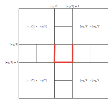
To test how dependent the algorithm is on the stretch of the ST, we also look at a special ST for $n_{1}\times n_{2}$ grids. As depicted in Figure 1, we construct this spanning tree by subdividing the $n_{1}\times n_{2}$ grid into four subgrids as evenly as possible, recursively building the STs in the subgrids and connecting the subgrids by a U-shape in the middle.

Proposition 1

The special ST has $\mathcal{O}\bigl{(}\frac{(n_{1}+n_{2})^{2}\log(n_{1}+n_{2})}{n_{1}n_{2}}\bigr{)}$ average stretch on an $n_{1}\times n_{2}$ grid.

Flows on trees.

Since every basis cycle contains exactly one off-tree-edge, the flows on off-tree-edges can simply be stored in a single vector. To be able to efficiently get the potential drop of every basis cycle and to be able to add a constant amount of flow to it, the core problem is to efficiently store and update flows in $T$. More formally, we want to support the following two operations for all $u,v\in V$ and $\alpha\in\real$ on the flow $f$:

• $\operatorname{query}(u,v)$: return the potential drop $\sum_{e\in P_{T}(u,v)}f(e)r_{e}$

• $\operatorname{update}(u,v,\alpha)$: set $f(e):=f(e)+\alpha$ for all $e\in P_{T}(u,v)$

We can simplify the operations by fixing $v$ to be the root $r$ of $T$: $\operatorname{query}(u)$: return the potential drop $\sum_{e\in P_{T}(u,r)}f(e)r_{e}$ and $\operatorname{update}(u,\alpha)$: set $f(e):=f(e)+\alpha$ for all $e\in P_{T}(u,r)$. The itemized two-node operations can then be supported with $\operatorname{query}(u,v):=\operatorname{query}(u)-\operatorname{query}(v)$ and $\operatorname{update}(u,v,\alpha):=\bigl{\{}\operatorname{update}(u,\alpha)\text{\,and}\operatorname{update}(v,-\alpha)\bigr{\}}$ since the changes on the subpath $P_{T}\bigl{(}r,\operatorname{LCA}(u,v)\bigr{)}$ cancel out. Here $\operatorname{LCA}(u,v)$ is the lowest common ancestor of the nodes $u$ and $v$ in $T$, the node farthest from $r$ that is an ancestor of both $u$ and $v$. We provide two approaches for implementing the operations, first an implementation of the one-node operations that stores the flow directly on the tree and uses the definitions of the operations without modification. Obviously, these operations require $\mathcal{O}(n)$ worst-case time and $\mathcal{O}(n)$ space. With an LCA data structure, one can implement the itemized two-node operations without the subsequent simplification of using one-node operations. This does not improve the worst-case time, but can help in practice. Secondly, we use the improved data structure by Kelner et al. [14] that guarantees $\mathcal{O}(\log n)$ worst-case time but uses $\mathcal{O}(n\log n)$ space. In this case the one-node operations boil down to a dot product ($\operatorname{query}$) and an addition ($\operatorname{update}$) of a dense vector and a sparse vector. We unroll the recursion within the data structure for better performance in practice.

Cycle selection.

The easiest way to select a cycle is to choose an off-tree edge uniformly at random in $\mathcal{O}(1)$ time. However, to get provably good results, we need to weight the off-tree-edges by their stretch. We can use the flow data structure described above to get the stretches. More specifically, the data structure initially represents $f=0$. For every off-tree edge $uv$ we first execute $\operatorname{update}(u,v,1)$, then $\operatorname{query}(u,v)$ to get $\sum_{e\in P_{T}(u,v)}r_{e}$ and finally $\operatorname{update}(u,v,-1)$ to return to $f=0$. This results in $\mathcal{O}(m\log n)$ time to initialize cycle selection. Once we have the weights, we use roulette wheel selection in order to select a cycle in $\mathcal{O}(\log m)$ time after an additional $\mathcal{O}(m)$ time initialization.

For convenience we summarize the implementation choices for Algorithm 1 in Table 2 (appendix). The top-level item in each section is the running time of the best sub-item that can be used to get a provably good running time. The convergence theorem requires a low-stretch spanning tree and weighted cycle selection. Note that $m=\Omega(n)$ as $G$ is connected.

4 Evaluation

4.1 Settings

We implemented the KOSZ solver in C++ using NetworKit [26], a toolkit focused on scalable network analysis algorithms. As compiler we use g++ 4.8.3. The benchmark platform is a dual-socket server with two 8-core Intel Xeon E5-2680 at 2.7 GHz each and 256 GB RAM. Only a representative subset of our experiments are shown here. More experiments and their detailed discussion can be found in [13]. We compare our KOSZ implementation to existing linear solvers as implemented by the libraries Eigen 3.2.2 [12] and Paralution 0.7.0 [18]. CPU performance characteristics such as the number of executed FLOPS (floating point operations), etc. are measured with the PAPI library [7].

We mainly use two graph classes for our tests: (i) Rectangular $k\times l$ grids given by $\mathbb{G}_{k,l}:=\bigl{(}[k]\times[l],\bigl{\{}\{(x_{1},y_{1}),(x_{2},y_{2})\}\subseteq\binom{V}{2}:|x_{1}-x_{2}|=1\lor|y_{1}-y_{2}|=1\bigr{\}}\bigr{)}$. Laplacian systems on grids are, for example, crucial for solving boundary value problems on rectangular domains; (ii) Barabási-Albert [4] random graphs with parameter $k$. These random graphs are parametrized with a so-called attachment $k$. Their construction models that the degree distribution in many natural graphs is not uniform at all. For both classes of graphs, we consider both unweighted and weighted variants (uniform random weights in $[1,8)$). We also did informal tests on 3D grids and graphs that were not generated synthetically. These graphs did not exhibit significantly different behavior than the two graph classes above.

4.2 Results

Spanning tree.

Figure 2: Average stretch $\operatorname{st}(T)/m$ with different ST algorithms.

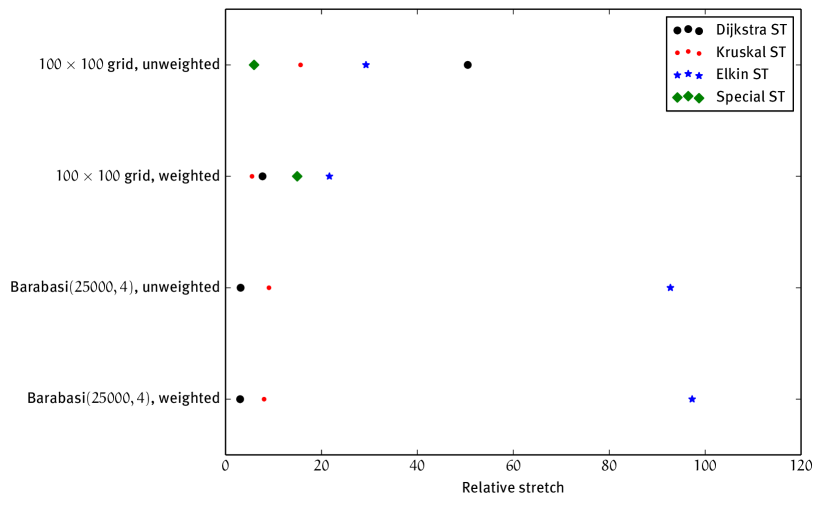
Papp [20] tested various low-stretch spanning tree algorithms and found that in practice the provably good low-stretch algorithms do not yield better stretch than simply using Kruskal. We confirm and extend this observation by comparing our own implementation of Elkin et al.’s [11] low-stretch ST algorithm to Kruskal and Dijkstra in Figure 2. Except for the unweighted $100\times 100$ grid, Elkin has worse stretch than the other algorithms and Kruskal yields a good ST. For Barabási-Albert graphs, Elkin is extremely bad (almost factor $20$ worse). Interestingly, Kruskal outperforms the other algorithms even on the unweighted Barabási-Albert graphs, where it degenerates to choosing an arbitrary ST. Figure 2 also shows that our special ST yields significantly lower stretch for the unweighted 2D grid, but it does not help in the weighted case.

Convergence.

(a) $100\times 100$ grid, unweighted

(b) $100\times 100$ grid, weighted

Figure 3: Convergence of the residual. Terminate when residual $\leq 10^{-4}$.

(c) Barabási-Albert, $n=25000$, unweighted

(d) Barabási–Albert, $n=25000$, weighted

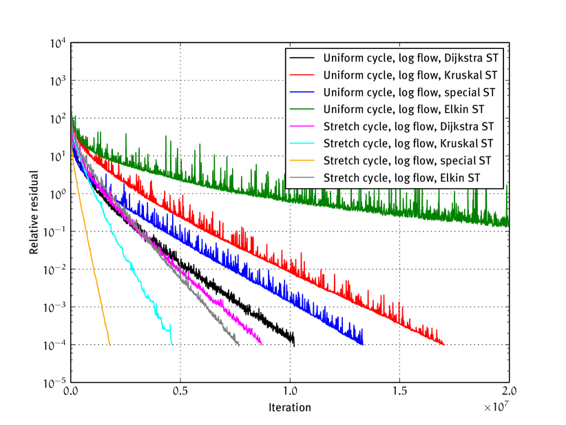
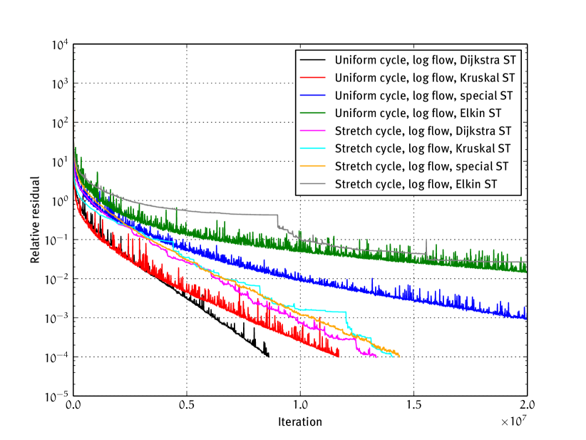
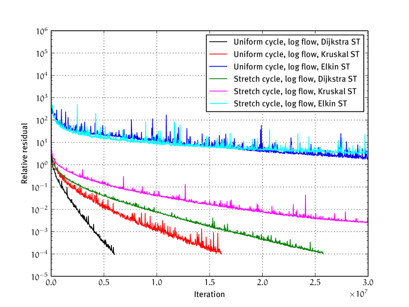
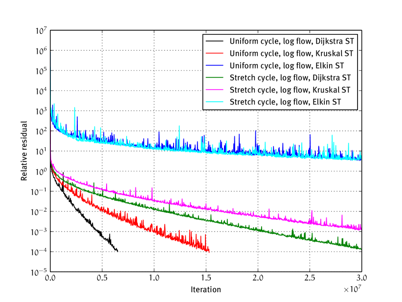
In Figure 3(b) we plot the convergence of the residual for different graphs and different algorithm settings. We examined a $100\times 100$ grid and a Barabási-Albert graph with $25,\!000$ nodes. While the residuals can increase, they follow a global downward trend. Also note that the spikes of the residuals are smaller if the convergence is better. In all cases the solver converges exponentially, but the convergence speed crucially depends on the solver settings. If we select cycles by their stretch, the order of the convergence speeds is the same as the order of the stretches of the ST (cmp. Figure 2), except for the Dijkstra ST and the Kruskal ST on the weighted grid. In particular, for the Elkin ST on Barabási-Albert graphs, there is a significant gap to the other settings where the solver barely converges at all and the special ST wins. Thus, low-stretch STs are crucial for convergence. In informal experiments we also saw this behavior for 3D grids and non-synthetic graphs.

We could not detect any correlation between the improvement made by a cycle repair and the stretch of the cycle. Therefore, we cannot fully explain the different speeds with uniform cycle selection and stretch cycle selection. For the grid the stretch cycle selection wins, while Barabási-Albert graphs favor uniform cycle selection. Another interesting observation is that most of the convergence speeds stay constant after an initial fast improvement at the start to about residual $1$. That is, there is no significant change of behavior or periodicity. Even though we can hugely improve convergence by choosing the right settings, even the best convergence is still very slow, e.g. we need about $6$ million iterations ($\approx 3000$ sparse matrix-vector multiplications (SpMVs) in time comparison) on a Barabási-Albert graph with $25,\!000$ nodes and $100,\!000$ edges in order to reach residual $10^{-4}$. In contrast, conjugate gradient (CG) without preconditioning only needs $204$ SpMVs for this graph.

Asymptotics.

(a) Wall time

(b) Cycles

(c) FLOPS

(d) Memory accesses

Figure 4: Asymptotic behaviour for $2D$ grids. Termination when relative residual was $\leq 10^{-4}$. The error bars give the standard deviation.

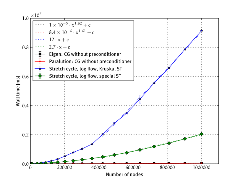
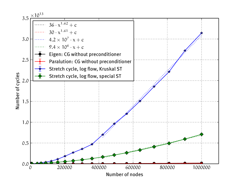
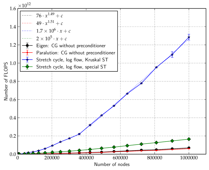
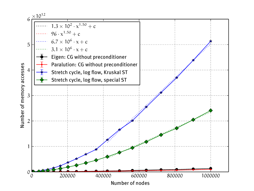
Now that we know which settings of the algorithm yield the best performance for 2D grids and Barabási-Albert graphs, we proceed by looking at how the performance with these settings behaves asymptotically and how it compares to conjugate gradient (CG) without preconditioning, a simple and popular iterative solver. Since KOSZ turns out to be not competitive, we do not need to compare it to more sophisticated algorithms.

In Figure 4 each occurrence of $c$ stands for a new instance of a real constant. We expect the cost of the CG method to scale with $\mathcal{O}(n^{1.5})$ on 2D grids [9], while our algorithm should scale nearly-linearly. This expectation is confirmed in the plot: Using Levenberg-Marquardt [19] to approximate the curves for CG with a function of the form $ax^{b}+c$, we get $b\approx 1.5$ for FLOPS and memory accesses, while the (more technical) wall time and cycle count yield a slightly higher exponent $b\approx 1.6$. We also see that the curves for our algorithm are almost linear from about $650\times 650$. Unfortunately, the hidden constant factor is so large that our algorithm cannot compete with CG even for a $1000\times 1000$ grid. Note that the difference between the algorithms in FLOPS is significantly smaller than the difference in memory accesses and that the difference in running time is larger still. This suggests that the practical performance of our algorithm is particularly bounded by memory access patterns and not by floating point operations. This is noteworthy when we look at our special spanning tree for the 2D grid. We see that using the special ST always results in performance that is better by a constant factor. In particular, we save a lot of FLOPS (factor $10$), while the savings in memory accesses (factor $2$) are a lot smaller. Even though the FLOPS when using the special ST are within a factor of $2$ of CG, we still have a wide chasm in running time.

The results for the Barabási-Albert graphs are basically the same (and hence not shown in detail): Even though the growth is approximately linear from about $400,\!000$ nodes, there is still a large gap between our algorithm and CG since the constant factor is enormous. Also, the results for the number of FLOPS are again much better than the result for the other performance counters. In conclusion, although we have nearly-linear growth, even for $1,\!000,\!000$ graph nodes, the KOSZ algorithm is still not competitive with CG because of huge constant factors, in particular a large number of iterations and memory accesses.

Smoothing.

One way of combining the good qualities of two different solvers is smoothing. Smoothing means to dampen the high-frequency components of the error, which is usually done in combination with another solver that dampens the low-frequency error components. It is known that in CG and most other solvers, the low-frequency components of the error converge very fast, while the high-frequency components converge slowly. Thus, we are interested in finding an algorithm that dampens the high-frequency components, a good smoother. This smoother does not necessarily need to reduce the error, it just needs to make its frequency distribution more favorable. Smoothers are particularly often applied at each level of multigrid or multilevel schemes [6] that turn a good smoother into a good solver by applying it at different levels of a matrix hierarchy. To test whether the Laplacian solver is a good smoother, we start with a fixed $x$ with $Lx=b$ and add white uniform noise in $[-1,1]$ to each of its entries in order to get an initial vector $x_{0}$. Then we execute a few iterations of our Laplacian solver and check whether the high-frequency components of the error have been reduced. Unfortunately, we cannot directly start at the vector $x_{0}$ in the solver. Our solution is to use Richardson iteration. That is, we transform the residual $r=b-Lx_{0}$ back to the source space by computing $L^{-1}r$ with the Laplacian solver, get the error $e=x-x_{0}=L^{-1}r$ and then the output solution $x_{1}=x_{0}+L^{-1}r.$

(a) Initial error

(b) Initial frequency

(c) 1 iteration, error

(d) 1 iteration, frequency

(e) 10 iterations, error

(f) 10 iterations, frequency

(g) 100 iterations, error

(h) 100 iterations, frequency

(i) 1000 iterations, error

(j) 1000 iterations, frequency

(k) 10000 iterations, error

(l) 10000 iterations, frequency

Figure 5: The Laplacian solver with the special ST as a smoother on a $32\times 32$ grid. For each number of iterations of the solver we plot the current error and the absolute values of its transformation into the frequency domain. Note that (a) and (k) have a different scale.

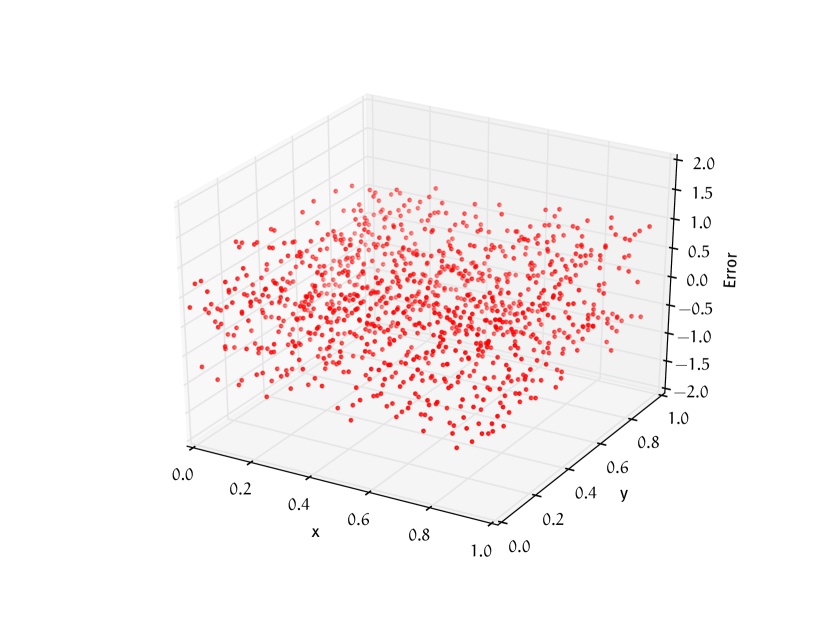
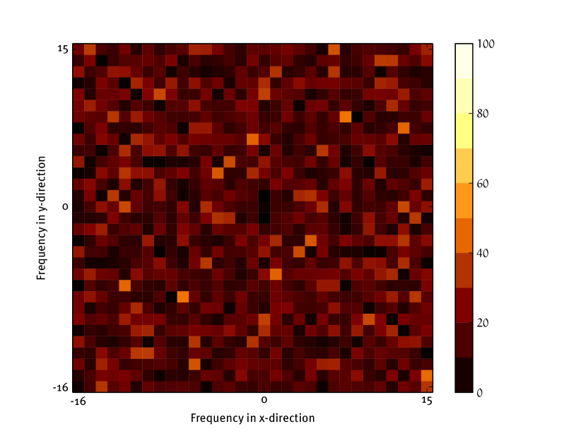
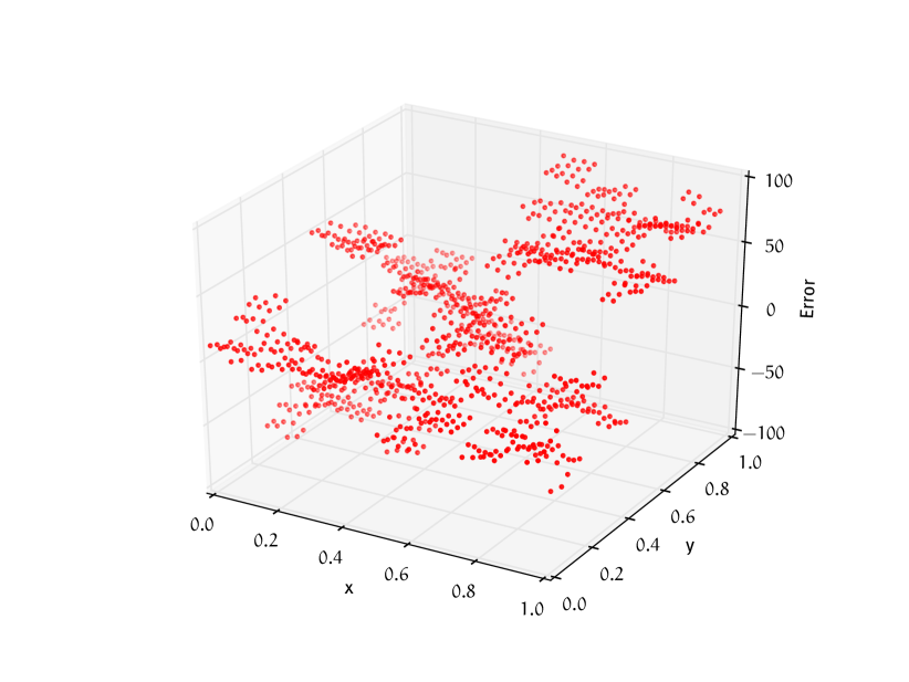
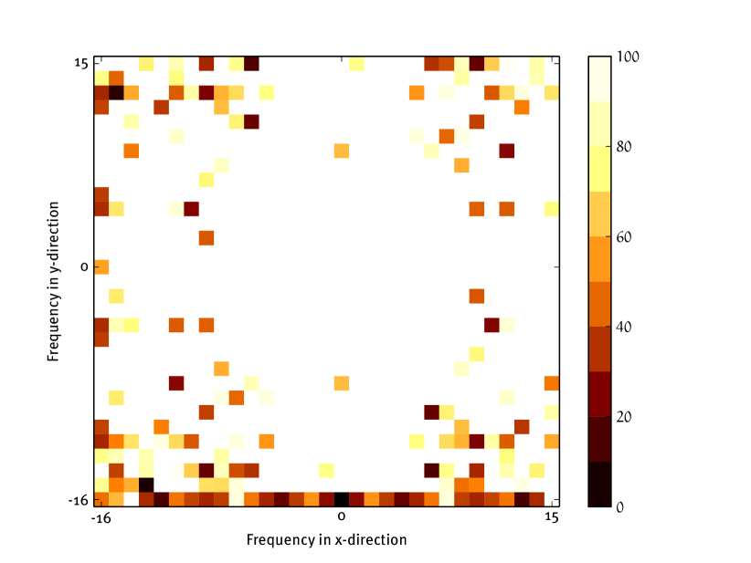
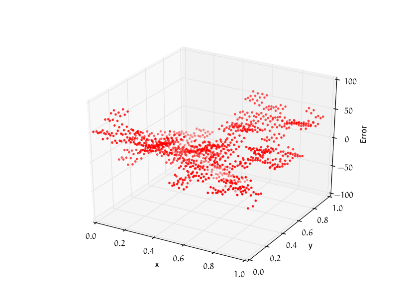
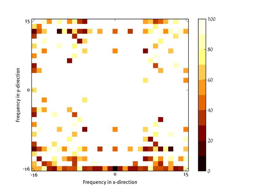
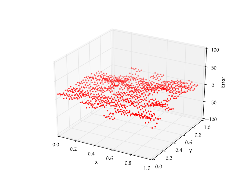
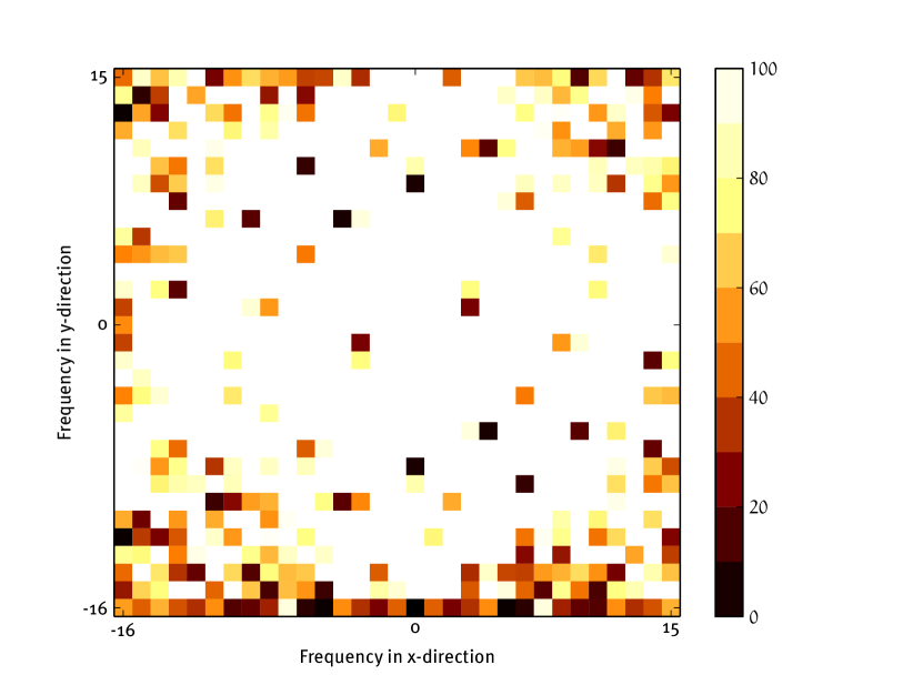
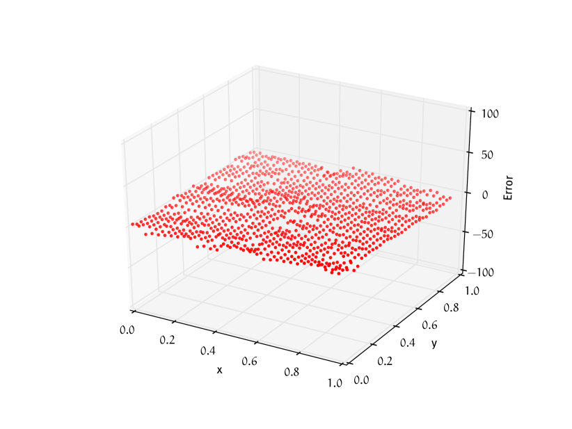
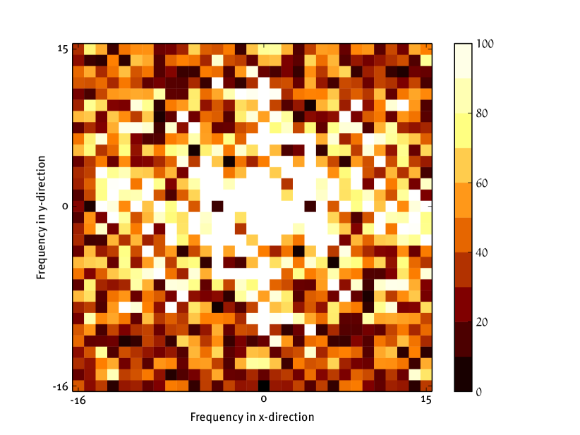
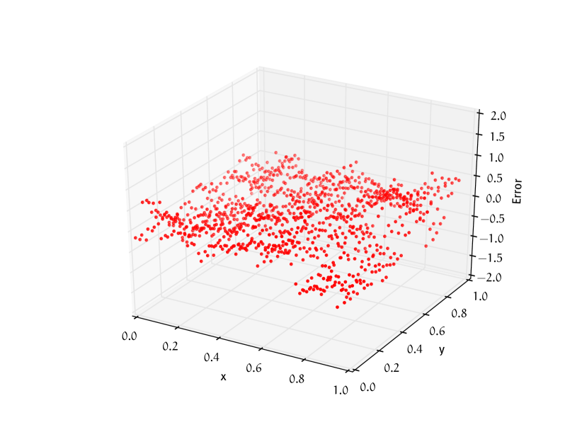
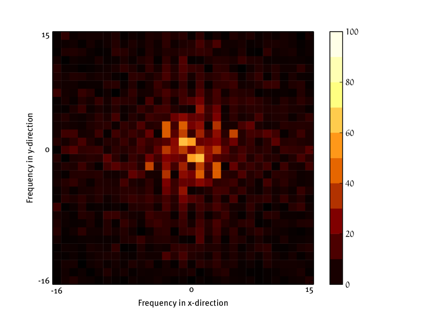
Figure 5 shows the error vectors of the solver for a $32\times 32$ grid together with their transformations into the frequency domain for different numbers of iterations of our solver. We see that the solver may indeed be useful as a smoother since the energies for the large frequencies (on the periphery) decrease rapidly, while small frequencies (in the middle) in the error remain.

In the solver we start with a flow that is nonzero only on the ST. Therefore, the flow values on the ST are generally larger at the start than in later iterations, where the flow will be distributed among the other edges. Since we construct the output vector by taking potentials on the tree, after one iteration $x_{1}$ will, thus, have large entries compared to the entries of $b$. In subplot (c) of Figure 5 we see that the start vector of the solver has the same structure as the special ST and that its error is very large. For the $32\times 32$ grid we, therefore, need about $10000$ iterations ($\approx 150$ SpMVs in running time comparison) to get an error of $x_{1}$ similar to $x_{0}$ even though the frequency distribution is favorable. Note that the number of SpMVs the $10000$ iterations correspond to depends on the graph size, e.g. for an $100\times 100$ grid the $10000$ iterations correspond to $20$ SpMVs.

While testing the Laplacian solver in a multigrid scheme could be worthwhile, the bad initial vector creates robustness problems when applying the Richardson iteration multiple times with a fixed number of iterations of our solver. In informal tests multiple Richardson steps lead to ever increasing errors without improved frequency behavior unless our solver already yields an almost perfect vector in a single run.

5 Conclusions

At the time of writing, the presented KOSZ [14] implementation and evaluation provide the first comprehensive experimental study of a Laplacian solver with provably nearly-linear running time. Our study supports the theoretical result that the convergence of KOSZ crucially depends on the stretch of the chosen spanning tree, with low stretch generally resulting in faster convergence. This particularly suggests that it is crucial to build algorithms that yield spanning trees with lower stretch. Since we have confirmd and extended Papp’s [20] observation that algorithms with provably low stretch do not yield good stretch in practice, improving the low-stretch ST algorithms is an important future research direction. Even though KOSZ proves to grow nearly linearly as predicted by theory, the constant seems to be too large to make it competitive, even compared to the CG method without preconditioner. Hence, our initial question in the paper title can be answered with “yes” and “no” at the same time: The running time is nearly linear, but the constant factors prevent usefulness in practice. While the negative results may predominate, our effort is the first to provide an answer at all. We hope to deliver insights that lead to further improvements, both in theory and practice. A promising future research direction is to repair cycles other than just the basis cycles in each iteration, but this would necessitate significantly different data structures.

Appendix

Appendix 0.A KOSZ Solver Background

0.A.1 Correspondence between Graphs and Laplacian Matrices

Table 1: Interpretations given to a Laplacian $L=L(G)\in{}^{n\times n}$ and a vector $x\in{}^{n}$ where the $w_{e}$ for each $e\in E$ are the edge weights.

$e$	edge/resistor $e$
$w_{e}$	conductance of resistor $e$
$r_{e}:=1/w_{e}$	resistance of resistor $e$
$x_{u}$	potential at node $u$
$(Lx)_{u}$	current flowing out of node $u$
$b_{u}$	current required to flow out of node $u$

$L$ operates on every vector $x\in{}^{n}$ via

$$(Lx)_{u} =-x_{u}\cdot\sum_{v\in N(u)}w_{uv}+\sum_{v\in N(u)}x_{v}\cdot w_{uv}$$

$$=\sum_{v\in N(u)}(x_{v}-x_{u})\cdot w_{uv}$$

for each $u\in V$.

Figure 6: Transformation into an electrical network.

0.A.2 Algorithm Components

Table 2: Summary of the components of the algorithm

Spanning tree	$\mathcal{O}\bigl{(}m\log n\log\log n)\bigr{)}$ stretch, $\mathcal{O}(m\log n\log\log n)$ time
Dijkstra	no stretch bound, $\mathcal{O}(m\log n)$ time
Kruskal	no stretch bound, $\mathcal{O}(m\log n)$ time
Elkin et. al. [11]	$\mathcal{O}(m\log^{2}\!n\log\log n)$ stretch, $\mathcal{O}(m\log^{2}\!n)$ time
Abraham et. al. [2]	$\mathcal{O}(m\log n\log\log n)$ stretch, $\mathcal{O}(m\log n\log\log n)$ time
Initialize cycle selection	$\mathcal{O}(m\log n)$ time
Uniform	$\mathcal{O}(m)$ time
Weighted	$\mathcal{O}(m\log n)$ time
Initialize flow	$\mathcal{O}(n\log n)$ time
LCA flow	$\mathcal{O}(n)$ time
Log flow	$\mathcal{O}(n\log n)$ time
Iterations	$\mathcal{O}\bigl{(}m\log n\log\log n\log(\epsilon^{-1}\log n)\bigr{)}$ expected iterations
Select a cycle	$\mathcal{O}(\log n)$ time
Uniform	$\mathcal{O}(1)$ time
Weighted	$\mathcal{O}(\log n)$ time
Repair cycle	$\mathcal{O}(\log n)$ time
LCA flow	$\mathcal{O}(n)$ time
Log flow	$\mathcal{O}(\log n)$ time
Complete solver	$\mathcal{O}(m\log^{2}\!n\log\log n\log\bigl{(}\epsilon^{-1}\log n)\bigr{)}$ expected time
Improved solver	$\mathcal{O}(m\log^{2}\!n\log\log n\log\bigl{(}\epsilon^{-1})\bigr{)}$ expected time

Appendix 0.B Spanning Tree Results

0.B.1 Proof of Proposition 1

We can inductively show that the average stretch $S(n_{1},n_{2})$ of the special ST on the $n_{1}\times n_{2}$ grid is in $\mathcal{O}\bigl{(}(n_{1}+n_{2})^{2}\log(n_{1}+n_{2})/n_{1}n_{2}\bigr{)}$. To do so, we first prove that by the recursive construction the distance of a node on a border of the grid to a corner of the same border is in $\mathcal{O}(n_{1}+n_{2})$. Thus, the stretches of the $n_{1}+n_{2}-3$ off-tree edges between the rows $\lfloor n_{2}/2\rfloor$ and $\lfloor n_{2}/2\rfloor+1$ as well as the columns $\lfloor n_{1}/2\rfloor$ and $\lfloor n_{1}/2\rfloor+1$ are in $\mathcal{O}(n_{1}+n_{2})$ each. Consequently,

$$S\bigl{(}n_{1},n_{2}\bigr{)}=4\cdot S\bigl{(}n_{1}/2,n_{2}/2\bigr{)}+\mathcal{O}\bigl{(}n_{1}+n_{2}\bigr{)}^{2}$$

when disregarding rounding. After solving this recurrence (note that $S(n_{1}/2,n_{2}/2)$ is essentially one fourth in size compared to $S(n_{1},n_{2})$), we get

$$S\bigl{(}n_{1},n_{2}\bigr{)}=\mathcal{O}\bigl{(}(n_{1}+n_{2})^{2}\log(n_{1}+n_{2})\bigr{)}.$$

Since the number of edges of the grid is $\Theta(mn)$, the claim for the average stretch follows. Note that in case of a square grid ($n_{1}=n_{2}$) with $N=n_{1}\times n_{2}$ vertices, we get

$$S(N)=4S(N/4)+\mathcal{O}(N)=\mathcal{O}(N\log N)=\mathcal{O}(n_{1}^{2}\log(n_{1}))$$

and thus $\mathcal{O}(\log n_{1})$ average stretch. ∎

0.B.2 Overview of spanning tree algorithms and their stretch

Table 3: Spanning tree algorithms and their guaranteed stretch

	Time	Stretch
[3]	$\mathcal{O}\bigl{(}m^{2}\bigr{)}$	$m\cdot exp\bigl{(}\mathcal{O}(\sqrt{\log n\log\log n})\bigr{)}$
[11]	$\mathcal{O}\bigl{(}m\log^{2}\!n\bigr{)}$	$m\cdot\mathcal{O}\bigl{(}\log^{2}\!n\log\log n\bigr{)}$
[1]	$\mathcal{O}\bigl{(}m\log^{2}\!n\bigr{)}$	$m\cdot\mathcal{O}\bigl{(}\log n(\log\log n)^{3}\bigr{)}$
[17]	$\mathcal{O}\bigl{(}m\log n\log\log n\bigr{)}$	$m\cdot\mathcal{O}\bigl{(}\log n(\log\log n)^{3}\bigr{)}$
[2]	$\mathcal{O}\bigl{(}m\log n\log\log n\bigr{)}$	$m\cdot\mathcal{O}\bigl{(}\log n\log\log n\bigr{)}$
Dijkstra	$\mathcal{O}\bigl{(}(m+n)\log n\bigr{)}$	No guarantee
Kruskal	$\mathcal{O}\bigl{(}m\alpha(n)\log n\bigr{)}$	No guarantee

References

- [1] I. Abraham, Y. Bartal, and O. Neiman. Nearly tight low stretch spanning trees. In 49th Annual Symposium on Foundations of Computer Science, pages 781–790, 2008.
- [2] Ittai Abraham and Ofer Neiman. Using petal-decompositions to build a low stretch spanning tree. In 44th ACM Symposium on Theory of Computing, pages 395–406, 2012.
- [3] Noga Alon, Richard M. Karp, David Peleg, and Douglas West. A graph-theoretic game and its application to the k-server problem. SIAM Journal on Computing, 24:78–100, 1995.
- [4] Albert-László Barabási and Réka Albert. Emergence of scaling in random networks. Science, 286(5439):509–512, 1999.
- [5] E. Boman, B. Hendrickson, and S. Vavasis. Solving elliptic finite element systems in near-linear time with support preconditioners. SIAM Journal on Numerical Analysis, 46(6):3264–3284, 2008.
- [6] William L. Briggs, Van Emden Henson, and Steve F. McCormick. A multigrid tutorial. SIAM, 2000.
- [7] S. Browne, J. Dongarra, N. Garner, G. Ho, and P. Mucci. A portable programming interface for performance evaluation on modern processors. Int. J. High Perform. Comput. Appl., 14(3):189–204, August 2000.
- [8] Paul Christiano, Jonathan A. Kelner, Aleksander Madry, Daniel A. Spielman, and Shang-Hua Teng. Electrical flows, laplacian systems, and faster approximation of maximum flow in undirected graphs. In Proc. 43rd ACM Symp. on Theory of Computing (STOC), pages 273–282. ACM, 2011.
- [9] James W. Demmel. Applied Numerical Linear Algebra. Society for Industrial and Applied Mathematics, Philadelphia, PA, USA, 1997.
- [10] Ralf Diekmann, Andreas Frommer, and Burkhard Monien. Efficient schemes for nearest neighbor load balancing. Parallel Computing, 25(7):789–812, 1999.
- [11] Michael Elkin, Yuval Emek, Daniel A. Spielman, and Shang-Hua Teng. Lower-stretch spanning trees. In Proceedings of the Thirty-seventh Annual ACM Symposium on Theory of Computing, pages 494–503, New York, NY, USA, 2005. ACM.
- [12] Gaël Guennebaud, Benoît Jacob, et al. Eigen v3. http://eigen.tuxfamily.org, 2010.
- [13] Daniel Hoske. An experimental study of a nearly-linear time laplacian solver. Master’s thesis, Karlsruhe Institute of Technology (KIT), 2014.
- [14] Jonathan A. Kelner, Lorenzo Orecchia, Aaron Sidford, and Zeyuan Allen Zhu. A simple, combinatorial algorithm for solving sdd systems in nearly-linear time. In Proceedings of the Forty-fifth Annual ACM Symposium on Theory of Computing, pages 911–920, New York, NY, USA, 2013.
- [15] Ioannis Koutis. Simple parallel and distributed algorithms for spectral graph sparsification. In Proc. 26th ACM Symp. on Parallelism in algorithms and architectures (SPAA), pages 61–66. ACM, 2014.
- [16] Ioannis Koutis, Alex Levin, and Richard Peng. Improved spectral sparsification and numerical algorithms for sdd matrices. In Symposium on Theoretical Aspects of Computer Science, volume 14, pages 266–277, 2012.
- [17] Ioannis Koutis, Gary L. Miller, and Richard Peng. A nearly- time solver for sdd linear systems. In Proceedings of the 2011 IEEE 52nd Annual Symposium on Foundations of Computer Science, FOCS ’11, pages 590–598, Washington, DC, USA, 2011. IEEE Computer Society.
- [18] Dimitar Lukarski. Paralution - library for iterative sparse methods. 2015. http://www.paralution.com, last access: Feb 09, 2015.
- [19] D. Marquardt. An algorithm for least-squares estimation of nonlinear parameters. Journal of the Society for Industrial and Applied Mathematics, 11(2):431–441, 1963.
-
[20]
Pál András Papp.
\hrefhttp://www.cs.elte.hu/blobs/diplomamunkak/bsc_alkmat/2014/papp_pal_andras.pdfLow-Stretch
Spanning Trees, 2014.
Bachelor thesis,
Eötvös Loránd University. - [21] Richard Peng and Daniel A. Spielman. An efficient parallel solver for sdd linear systems. In Proceedings of the 46th Annual ACM Symposium on Theory of Computing, STOC ’14, pages 333–342, New York, NY, USA, 2014. ACM.
- [22] J.H. Reif. Efficient approximate solution of sparse linear systems. Computers & Mathematics with Applications, 36(9):37 – 58, 1998.
- [23] Daniel A. Spielman and Nikhil Srivastava. Graph sparsification by effective resistances. In STOC, STOC ’08, New York, NY, USA, 2008.
- [24] Daniel A. Spielman and Shang-Hua Teng. Nearly-linear time algorithms for graph partitioning, graph sparsification, and solving linear systems. In STOC, STOC ’04, pages 81–90, New York, NY, USA, 2004.
- [25] Daniel A. Spielman and Jaeoh Woo. A note on preconditioning by low-stretch spanning trees. CoRR, abs/0903.2816, 2009.
- [26] Christian L. Staudt, Aleksejs Sazonovs, and Henning Meyerhenke. Networkit: An interactive tool suite for high-performance network analysis. arXiv:1403.3005, 2014.
- [27] P. M. Vaidya. Solving linear equations with symmetric diagonally dominant matrices by constructing good preconditioners. Technical report, University of Illinois at Urbana-Champaign, Urbana, IL, 1990.