Fast and accurate prediction of numerical relativity waveforms from binary black hole coalescences using surrogate models
Abstract
Simulating a binary black hole (BBH) coalescence by solving Einstein’s equations is computationally expensive, requiring days to months of supercomputing time. Using reduced order modeling techniques, we construct an accurate surrogate model, which is evaluated in a millisecond to a second, for numerical relativity (NR) waveforms from non-spinning BBH coalescences with mass ratios in and durations corresponding to about orbits before merger. We assess the model’s uncertainty and show that our modeling strategy predicts NR waveforms not used for the surrogate’s training with errors nearly as small as the numerical error of the NR code. Our model includes all spherical-harmonic waveform modes resolved by the NR code up to We compare our surrogate model to Effective One Body waveforms from - for advanced LIGO detectors and find that the surrogate is always more faithful (by at least an order of magnitude in most cases).
Since the breakthroughs of 2005 Pretorius (2005); Campanelli et al. (2006); Baker et al. (2006), tremendous progress in numerical relativity (NR) has led to hundreds of simulations of binary black hole (BBH) coalescences Aylott et al. (2009); Ajith et al. (2012); Mroue et al. (2013); Hinder et al. (2014); Pekowsky et al. (2013); Aasi et al. (2014); SXS (a). This progress has been driven partly by data analysis needs of advanced ground-based gravitational wave detectors like LIGO Harry (2010) (for the LIGO Scientific Collaboration) and Virgo The Virgo Collaboration (2009). Recent upgrades to these detectors are expected to yield the first direct detections of gravitational waves (GWs) from compact binary coalescences Abadie et al. (2010).
Despite the remarkable progress of the NR community, a single high-quality simulation typically requires days to months of supercomputing time. This high computational cost makes it difficult to directly use NR waveforms for data analysis, except for injection studies Aylott et al. (2009); Aasi et al. (2014), since detecting GWs and inferring their source parameters may require thousands to millions of accurate gravitational waveforms. Nevertheless, a first template bank for nonspinning binaries in Advanced LIGO has been recently constructed from NR waveforms Kumar et al. (2014). Furthermore, NR waveforms have been used successfully in calibrating inspiral-merger-ringdown (IMR) effective-one-body (EOB) Buonanno and Damour (1999); Damour and Nagar (2009); Buonanno et al. (2009); Pan et al. (2010, 2011); Damour et al. (2013); Taracchini et al. (2012) and phenomenological Ajith et al. (2007); Santamaría et al. (2010); Sturani et al. (2010); Hannam et al. (2014) models. These models have free parameters that can be set by matching to NR waveforms and are suitable for certain GW data analysis studies Abadie et al. (2011). However, these models can have systematic errors since they assume a priori physical waveform structure and are calibrated and tested against a small set of NR simulations.
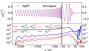
In this Letter, we present an ab initio methodology based on surrogate Field et al. (2014); Kaye (2012) and reduced order modeling techniques Maday et al. (2002); Veroy et al. (2003); Prud’homme et al. (2002); Chen et al. (2010); Quarteroni et al. (2011) that is capable of accurately predicting the gravitational waveform outputs from NR without any phenomenological assumptions or approximations to general relativity. From a small set of specially selected non-spinning BBH simulations performed with the Spectral Einstein Code (SpEC) SpE ; Scheel et al. (2015); Szilágyi (2014), we build a surrogate model that can be used in place of performing SpEC simulations. The techniques are general, however, and directly apply to other NR codes or even analytical waveform models. The surrogate model constructed here generates non-spinning BBH waveforms with mass ratios , contains – gravitational wave cycles before peak amplitude, and includes many spherical-harmonic modes (see Table 2 and its caption). These choices are made based on available NR waveforms and are not limitations of the method. Our surrogate model has errors close to the estimated numerical error of the input waveforms. An example comparing the surrogate output to an NR waveform can be seen in Fig. 1. This simulation took days using cores but only sec for the surrogate evaluation of the (2,2) mode.
Previous work Field et al. (2014); Pürrer (2014) built surrogates for EOB waveforms; building and assessing surrogate models of NR waveforms have unique challenges associated with input waveforms that are expensive to compute. We summarize next the construction of our model, focusing on steps not addressed in Field et al. (2014) but are required for NR surrogates.
Parametric sampling– Typically, a surrogate model is trained on a dense set of waveforms known as the training set. In the case of NR, we cannot afford to generate a large number of waveforms. Instead, we generate a dense set of non-spinning waveforms using an EOB model Pan et al. (2010), as implemented in Collaboration , which contains the spin-weight spherical-harmonic modes and captures robust features of NR waveforms. The EOB training set waveforms are computed for times in ( is the total mass), which is the interval over which we build our surrogates.
Next, on this training set we apply a greedy algorithm to expose the most relevant mass ratio values Binev et al. (2011); Field et al. (2011). The algorithm proceeds from a linear basis constructed from waveforms already chosen. The norms of the differences between the training set waveforms and their projection onto this basis are computed. The waveform with the largest such error is added to the basis as its element. SpEC simulations of non-spinning BBH mergers are then performed for these mass ratios. The resulting NR waveforms are used to build our surrogates without any further input from the EOB model.
We seeded the greedy algorithm with publicly available SpEC simulations of non-spinning BBH mergers Pan et al. (2011); SXS (a) (see Table 1), and the next (ordered) mass ratio values are the algorithm’s output based on the EOB model. The final mass ratios are included to improve the surrogate if necessary, since we can assess the surrogate model’s accuracy only after it is built. Our method for building surrogates is hierarchical Field et al. (2011, 2014); additional NR waveforms can be included to improve the model’s accuracy.
Generating the NR waveforms– Table 1 summarizes the SpEC simulations used in this paper. See, e.g., Ref. Scheel et al. (2015) for the numerical techniques used in SpEC. The numerical resolution is denoted by “Lev”, where is an integer that controls the local truncation error in the metric and its derivatives allowed by adaptive mesh refinement (AMR) in SpEC; larger numbers correspond to smaller errors (the error threshold scales like ) and more computationally-expensive simulations. The scaling of global quantities (e.g. waveform errors) with is difficult to estimate a priori. Two to five levels of resolution are simulated for each mass ratio. To achieve quasi-circular orbits, initial data are subject to an iterative eccentricity reduction procedure resulting in eccentricities Pfeiffer et al. (2007); Buonanno et al. (2011); Mroué and Pfeiffer (2012).
| ID | Orbs | ID | Orbs | ||||||||
|---|---|---|---|---|---|---|---|---|---|---|---|
SpEC numerically solves an initial boundary value problem defined on a finite computational domain. To obtain waveforms at future null infinity , we use the Cauchy characteristic extraction (CCE) method Bishop et al. (1997); Babiuc et al. (2011); Winicour (2009); Reisswig and Pollney (2011); Taylor et al. (2013). Using the PittNull code Bishop et al. (1997); Babiuc et al. (2011); Winicour (2009), we compute the Newman-Penrose scalar at and finally obtain the gravitational wave strain through two temporal integrations. We minimize the low-frequency, noise-induced “drifts” Reisswig and Pollney (2011) by using frequency cut-offs.111We integrate twice in the (dimensionless) frequency domain by dividing by , where is the initial GW mode frequency.
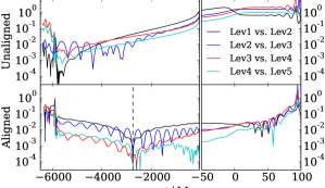
Figure 2 shows the convergence typically observed in our simulations when using AMR. Because AMR makes independent decisions for different Lev, a particular subdomain may sometimes have the same number of grid points for two different values of Lev at a given time, and the subdomain boundaries do not necessarily coincide for different Lev. Thus, plots like Figure 2 sometimes show anomalously small differences between particular pairs of numerical resolutions (for instance Lev2 vs. Lev3 near in the top panel of Figure 2). See Sec. IIIB of Scheel et al. (2015). Nevertheless, the waveform differences generally decrease quickly with increasing resolution. Let
| (1) |
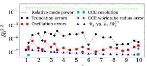
be the disagreement between two waveform modes and where . We estimate the numerical truncation error of each mode when and are waveforms computed at the two highest resolutions. The full waveform222 Throughout, we exclude modes because (non-oscillatory) Christodoulou memory is not accumulated sufficiently in current NR simulations Favata (2009). error for a given mass ratio is . We report numerical truncation errors after an overall simulation-dependent time shift and rotation (which we shall refer to as surrogate alignment, described in the next section), which are physically unimportant coordinate changes. The resulting estimated numerical truncation errors of the dominant modes, using our surrogate alignment scheme, are shown in Fig. 3 (black circles).
Additional error sources are non-zero eccentricity in the (intended to be circular) NR initial data, and an imperfect procedure for integrating to obtain . These both cause small oscillations in the waveform amplitudes and phases Reisswig and Pollney (2011); Mroué et al. (2010) that we model following Mroué et al. (2010). We also compute the error in the strain integration scheme by comparing to two time derivatives of , as well as estimates for numerical errors in the CCE method Taylor et al. (2013). For the mode, these additional errors are negligibly small compared to SpEC truncation errors (cf. Fig. 3).
Preparing NR waveforms for surrogate modeling– We apply a simulation-dependent time shift and physical rotation about the -axis so that all the modes’ phases are aligned. This reveals the underlying parametric smoothness in that will be useful for building a surrogate. Our time shifts set each waveform’s total amplitude
| (2) |
to be maximum at . After enforcing this alignment scheme we interpolate the waveform mode amplitudes and phases onto an array of uniformly spaced times in , with . Finally, we align the initial gravitational wave mode phases by performing a simulation-dependent, constant (in time) physical rotation about the -axis so that , which fixes a physical rotation up to multiples of . We resolve the ambiguity by requiring . Waveform truncation errors, after performing this surrogate alignment scheme, are shown in Fig. 2. In what follows, we call “truncation error after surrogate alignment” simply “truncation error.”
Building the surrogate– Each mode, , is modeled separately while (due to reflection symmetry about the orbital plane) modes are evaluated using . We model all modes but keep only those yielding smaller surrogate errors compared to setting the mode to zero. Table 2 lists our modeled modes and their errors.
Our complete surrogate waveform model is defined by where
| (3) | ||||
Unlike Ref. Field et al. (2014), we construct a reduced basis representation for the waveform amplitudes and phases separately, instead of the waveforms themselves Pürrer (2014). Here, the are computed off-line from the SpEC waveforms Field et al. (2014). At a set of specially selected times , which are the empirical interpolant nodes Maday et al. (2009); Field et al. (2014), the functions approximate the parametric variation of the amplitudes and phases (via fitting). A thorough discussion of surrogate model building steps is presented in Field et al. (2014). When evaluating the surrogate at a particular mass ratio, the fits are evaluated first to determine the amplitudes and phases at their respective interpolating times . The remaining operations yield the surrogate model prediction, .
To find each we perform least-squares fits to the data points, . All fits except odd mode amplitudes use th degree polynomials in the symmetric mass ratio, . For odd modes, the amplitude approaches and its derivative with respect to diverges as (or ). Consequently, we use to account for this behavior. The waveform phases of odd modes at , which are undefined, are excluded when fitting for each .
Assessing surrogate errors– We next assess the surrogate’s predictive quality. To quantify the error in the surrogate model itself, as opposed to its usage in a data analysis study, we do not minimize the errors over relative time and phase shifts here.
A first test is a consistency check to reproduce the input SpEC waveforms used to build the surrogate. These errors are shown in Fig. 4 (red squares) and are comparable to or smaller than the largest SpEC truncation errors (black circles).
A more stringent test is the leave-one-out cross-validation (LOOCV) study Hastie et al. (2001). For each simulated mass ratio , we build a temporary trial surrogate using the other waveforms, evaluate the trial surrogate at , and compare the prediction with the SpEC waveform for . Hence, the trial surrogate’s error at should serve as an upper bound for the full surrogate trained on all waveforms. Repeating this process for all possible LOOCV tests333We omit the smallest and largest mass ratios here as the corresponding trial surrogates would extrapolate to their values. results in Fig. 4 (blue triangles). Despite the th trial surrogate having no information about the waveform at , the errors remain comparable to the largest SpEC truncation errors. The LOOCV errors are typically twice as large as the full surrogate ones confirming the former as bounds for the latter. Relative errors for selected modes are shown in Table 2. While weaker modes have larger relative errors, their power contribution is small enough that the error in the full surrogate waveform, , is nearly identical to the SpEC resolution error.
| Surrogate | NR | Surrogate | NR | ||||||
|---|---|---|---|---|---|---|---|---|---|
| Max | Mean | Max | Mean | Max | Mean | Max | Mean | ||
| 0.36 | 0.07 | 0.36 | 0.08 | 100 | 17 | 1.7 | 0.43 | ||
| 29 | 3.4 | 4.1 | 0.54 | 7.4 | 2.2 | 20 | 2.1 | ||
| 53 | 4.1 | 11 | 0.94 | All | 0.42 | 0.12 | 0.40 | 0.10 | |
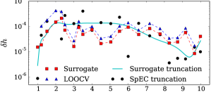
A third test is to compare the surrogate waveforms to those of a second surrogate, built from the second highest resolution SpEC waveforms. The resulting comparison is shown in Fig. 4 (cyan line). These errors are comparable to SpEC waveform truncation errors (black circles). We find that the surrogate building process is robust to resolution differences. Furthermore, the surrogate can be improved using NR waveforms of higher accuracy.
We perform a final test and construct surrogates using the first selected mass ratios (from Table 1) as input waveforms, leaving mass ratios with which to test. We find the total surrogate error decreases exponentially with and is comparable to the SpEC truncation error after using waveforms. Some modes (e.g., ) are fully resolved after as few as waveforms.
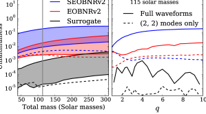
Comparison to EOB– For data analysis purposes, we compare our surrogate with EOBNRv2 Pan et al. (2011) and SEOBNRv2 Taracchini et al. (2012) models (generated from a current implementation444 We find that very small changes () in the minimum frequency or the total mass can have unexpectedly large changes in the unfaithfulness () in LAL Collaboration ). In Fig. 5, we show the unfaithfulness
| (4) |
of the surrogate and the two EOB models against the NR waveforms. Here, is the normalized Fourier transform of (such that a waveform’s unfaithfulness with itself gives ), and the advanced LIGO zero-detuned high power sensitivity noise curve Shoemaker (2010). The surrogate is more faithful than both EOB models for all cases considered. Since SEOBNRv2 only provides modes, it performs worst for large total masses where additional modes become important. All models predict the mode with an unfaithfulness for at , however the EOB models are limited by the availability of subdominant modes.
Discussion– We have built a surrogate model for NR non-spinning BBH merger waveforms generated by SpEC. On a standard 2015 single core computer, all modes with are evaluated in sec ( sec for a single mode) providing a factor of speedup compared to SpEC. Importantly, this is achieved with only a small loss in accuracy. Like other data-driven modeling strategies, our surrogate is valid only within the training intervals, namely, and . Therefore, within the training intervals, our surrogate model generates BBH merger waveforms that are equivalent to SpEC outputs up to numerical error and a small modeling error.
NR surrogates can be used for multiple-query applications in gravitational wave data analysis such as detector-specific template-bank (re-)generation and parameter estimation. Our surrogate, and more generally the results of this paper, open up the exciting possibility of performing, for example, parameter estimation with multi-modal NR waveforms (with hybridization, if needed). Parameter estimation studies seeking to incorporate model error may benefit from the surrogate’s relatively straightforward characterization and assessment of uncertainty from a combination of the surrogate’s and SpEC’s systematic and numerical errors. We anticipate NR surrogate modeling to complement traditional strategies Buonanno and Damour (1999); Ajith et al. (2007); Damour and Nagar (2009); Buonanno et al. (2009); Pan et al. (2010); Santamaría et al. (2010); Sturani et al. (2010); Pan et al. (2011); Abadie et al. (2011); Damour et al. (2013); Taracchini et al. (2012) by providing unlimited high-fidelity approximations of NR waveforms with which to calibrate, refine and make comparisons. Building NR surrogates of precessing BBH merger waveforms, which may be modeled from the parameters specially selected in Blackman et al. (2014), offer a promising avenue for modeling the full dimensional BBH parameter space. The surrogate model described in this paper is available for download at SXS (b); gws .
We thank Mike Boyle, Alessandra Buonanno, Collin Capano, Jan Hesthaven, Jason Kaye, Geoffrey Lovelace, Lee Lindblom, Tom Loredo, Christian Ott, Yi Pan, Harald Pfeiffer, Rory Smith, and Nicholas Taylor for many useful discussions throughout this project. This work was supported in part by NSF grants CAREER PHY-0956189, PHY-1068881, PHY-1005655, PHY-1440083, PHY-1404569, and AST-1333520 to Caltech, NSF grants PHY-1306125 and AST-1333129 to Cornell University, NSF grant PHY-1500818 to the University of California at San Diego, NSF grants PHY-1208861 and PHY-1316424 to the University of Maryland (UMD), NSERC of Canada, and the Sherman Fairchild Foundation. Computations were performed on the Zwicky cluster at Caltech, which is supported by the Sherman Fairchild Foundation and by NSF award PHY-0960291. Portions of this research were carried out at the Center for Scientific Computation and Mathematical Modeling cluster at UMD.
References
- Pretorius (2005) F. Pretorius, Phys. Rev. Lett. 95, 121101 (2005), arXiv:gr-qc/0507014 [gr-qc] .
- Campanelli et al. (2006) M. Campanelli, C. Lousto, P. Marronetti, and Y. Zlochower, Phys. Rev. Lett. 96, 111101 (2006), arXiv:gr-qc/0511048 [gr-qc] .
- Baker et al. (2006) J. G. Baker, J. Centrella, D.-I. Choi, M. Koppitz, and J. van Meter, Phys. Rev. Lett. 96, 111102 (2006), arXiv:gr-qc/0511103 [gr-qc] .
- Aylott et al. (2009) B. Aylott, J. G. Baker, W. D. Boggs, M. Boyle, P. R. Brady, et al., Class. Quant. Grav. 26, 165008 (2009), arXiv:0901.4399 [gr-qc] .
- Ajith et al. (2012) P. Ajith, M. Boyle, D. A. Brown, B. Brugmann, L. T. Buchman, et al., Class. Quantum Grav. 29, 124001 (2012).
- Mroue et al. (2013) A. H. Mroue, M. A. Scheel, B. Szilagyi, H. P. Pfeiffer, M. Boyle, D. A. Hemberger, L. E. Kidder, G. Lovelace, S. Ossokine, N. W. Taylor, A. Zenginoglu, L. T. Buchman, T. Chu, E. Foley, M. Giesler, R. Owen, and S. A. Teukolsky, Phys. Rev. Lett. 111, 241104 (2013), arXiv:1304.6077 [gr-qc] .
- Hinder et al. (2014) I. Hinder et al. (The NRAR Collaboration), Classical and Quantum Gravity 31, 025012 (2014), arXiv:1307.5307 [gr-qc] .
- Pekowsky et al. (2013) L. Pekowsky, R. O’Shaughnessy, J. Healy, and D. Shoemaker, Phys. Rev. D 88, 024040 (2013), arXiv:1304.3176 [gr-qc] .
- Aasi et al. (2014) J. Aasi et al. (The LIGO Scientific Collaboration, the Virgo Collaboration, the NINJA-2 Collaboration), Class. Quantum Grav. 31, 115004 (2014), arXiv:1401.0939 [gr-qc] .
- SXS (a) http://www.black-holes.org/waveforms (a).
- Harry (2010) (for the LIGO Scientific Collaboration) G. M. Harry (for the LIGO Scientific Collaboration), Class. Quantum Grav. 27, 084006 (2010).
- The Virgo Collaboration (2009) The Virgo Collaboration, “Advanced Virgo Baseline Design,” (2009), [VIR-0027A-09].
- Abadie et al. (2010) J. Abadie, B. P. Abbott, R. Abbott, M. Abernathy, T. Accadia, F. Acernese, C. Adams, R. Adhikari, P. Ajith, B. Allen, and et al., Classical and Quantum Gravity 27, 173001 (2010), arXiv:1003.2480 [astro-ph.HE] .
- Kumar et al. (2014) P. Kumar, I. MacDonald, D. Brown, H. Pfeiffer, K. Cannon, M. Boyle, L. Kidder, A. Mroue, M. Scheel, B. Szilagyi, and A. Zenginoglu, Phys. Rev. D 89, 042002 (2014), 1310.7949 .
- Buonanno and Damour (1999) A. Buonanno and T. Damour, Phys. Rev. D 59, 084006 (1999), arXiv:gr-qc/9811091 [gr-qc] .
- Damour and Nagar (2009) T. Damour and A. Nagar, Phys. Rev. D 79, 081503 (2009), arXiv:0902.0136 [gr-qc] .
- Buonanno et al. (2009) A. Buonanno, Y. Pan, H. P. Pfeiffer, M. A. Scheel, L. T. Buchman, and L. E. Kidder, Phys. Rev. D 79, 124028 (2009), arXiv:0902.0790 [gr-qc] .
- Pan et al. (2010) Y. Pan, A. Buonanno, L. T. Buchman, T. Chu, L. E. Kidder, H. P. Pfeiffer, and M. A. Scheel, Phys. Rev. D 81, 084041 (2010), arXiv:0912.3466 [gr-qc] .
- Pan et al. (2011) Y. Pan, A. Buonanno, M. Boyle, L. T. Buchman, L. E. Kidder, et al., Phys. Rev. D 84, 124052 (2011), arXiv:1106.1021 [gr-qc] .
- Damour et al. (2013) T. Damour, A. Nagar, and S. Bernuzzi, Phys.Rev. D87, 084035 (2013), arXiv:1212.4357 [gr-qc] .
- Taracchini et al. (2012) A. Taracchini, Y. Pan, A. Buonanno, E. Barausse, M. Boyle, T. Chu, G. Lovelace, H. P. Pfeiffer, and M. A. Scheel, Phys. Rev. D 86, 024011 (2012), arXiv:1202.0790 [gr-qc] .
- Ajith et al. (2007) P. Ajith, S. Babak, Y. Chen, M. Hewitson, B. Krishnan, J. T. Whelan, B. Brügmann, P. Diener, J. Gonzalez, M. H. S. Husa, M. Koppitz, D. Pollney, L. Rezzolla, L. Santamaría, A. M. Sintes, U. Sperhake, and J. Thornburg, Class. Quantum Grav. 24, S689 (2007), arXiv:0704.3764 [gr-qc] .
- Santamaría et al. (2010) L. Santamaría, F. Ohme, P. Ajith, B. Brügmann, N. Dorband, M. Hannam, S. Husa, P. Mösta, D. Pollney, C. Reisswig, E. L. Robinson, J. Seiler, and B. Krishnan, Phys. Rev. D 82, 064016 (2010), arXiv:1005.3306 [gr-qc] .
- Sturani et al. (2010) R. Sturani, S. Fischetti, L. Cadonati, G. Guidi, J. Healy, et al., J.Phys.Conf.Ser. 243, 012007 (2010), arXiv:1005.0551 [gr-qc] .
- Hannam et al. (2014) M. Hannam, P. Schmidt, A. Bohé, L. Haegel, S. Husa, et al., Phys.Rev.Lett. 113, 151101 (2014), arXiv:1308.3271 [gr-qc] .
- Abadie et al. (2011) J. Abadie et al. (The LIGO Scientific Collaboration and the Virgo Collaboration), Phys. Rev. D 83, 122005 (2011), arXiv:1102.3781 [gr-qc] .
- Field et al. (2014) S. E. Field, C. R. Galley, J. S. Hesthaven, J. Kaye, and M. Tiglio, Phys. Rev. X 4, 031006 (2014), arXiv:1308.3565 [gr-qc] .
- Kaye (2012) J. Kaye, The interpolation of gravitational waveforms, Ph.D. thesis, Brown University (2012).
- Maday et al. (2002) Y. Maday, A. T. Patera, and G. Turinici, J. Sci. Comput. 17, 437 (2002).
- Veroy et al. (2003) K. Veroy, C. Prud’homme, and A. T. Patera, Comptes Rendus Mathematique 337, 619 (2003).
- Prud’homme et al. (2002) C. Prud’homme, D. V. Rovas, K. Veroy, L. Machiels, Y. Maday, A. T. Patera, and G. Turinici, Journal of Fluids Engineering 124, 70 (2002).
- Chen et al. (2010) Y. Chen, J. S. Hesthaven, Y. Maday, and J. Rodríguez, SIAM J. Sci. Comput. 32, 970 (2010).
- Quarteroni et al. (2011) A. Quarteroni, G. Rozza, and A. Manzoni, Journal of Mathematics in Industry 1, 1 (2011).
- (34) http://www.black-holes.org/SpEC.html.
- Scheel et al. (2015) M. A. Scheel, M. Giesler, D. A. Hemberger, G. Lovelace, K. Kuper, M. Boyle, B. Szilágyi, and L. E. Kidder, Classical and Quantum Gravity 32, 105009 (2015), arXiv:1412.1803 [gr-qc] .
- Szilágyi (2014) B. Szilágyi, Int.J.Mod.Phys. D23, 1430014 (2014), arXiv:1405.3693 [gr-qc] .
- Pürrer (2014) M. Pürrer, Class. Quantum Grav. 31, 195010 (2014), arXiv:1402.4146 [gr-qc] .
- (38) L. S. Collaboration, “LSC Algorithm Library software packages lal, lalwrapper, and lalapps,” .
- Binev et al. (2011) P. Binev, A. Cohen, W. Dahmen, R. A. DeVore, G. Petrova, and P. Wojtaszczyk, SIAM J. Math. Analysis 43, 1457 (2011).
- Field et al. (2011) S. E. Field, C. R. Galley, F. Herrmann, J. S. Hesthaven, E. Ochsner, et al., Phys. Rev. Lett. 106, 221102 (2011), arXiv:1101.3765 [gr-qc] .
- Pfeiffer et al. (2007) H. P. Pfeiffer, D. A. Brown, L. E. Kidder, L. Lindblom, G. Lovelace, and M. A. Scheel, Class. Quantum Grav. 24, S59 (2007), gr-qc/0702106 .
- Buonanno et al. (2011) A. Buonanno, L. E. Kidder, A. H. Mroué, H. P. Pfeiffer, and A. Taracchini, Phys. Rev. D 83, 104034 (2011), arXiv:1012.1549 [gr-qc] .
- Mroué and Pfeiffer (2012) A. H. Mroué and H. P. Pfeiffer, (2012), arXiv:1210.2958 [gr-qc] .
- Bishop et al. (1997) N. T. Bishop, R. Gomez, L. Lehner, M. Maharaj, and J. Winicour, Phys. Rev. D56, 6298 (1997), arXiv:gr-qc/9708065 .
- Babiuc et al. (2011) M. C. Babiuc, B. Szilágyi, J. Winicour, and Y. Zlochower, Phys. Rev. D 84, 044057 (2011), arXiv:1011.4223 [gr-qc] .
- Winicour (2009) J. Winicour, Living Rev. Rel. 12 (2009).
- Reisswig and Pollney (2011) C. Reisswig and D. Pollney, Class. Quant. Grav. 28, 195015 (2011), arXiv:1006.1632 [gr-qc] .
- Taylor et al. (2013) N. W. Taylor, M. Boyle, C. Reisswig, M. A. Scheel, T. Chu, L. E. Kidder, and B. Szilágyi, Phys. Rev. D 88, 124010 (2013), arXiv:1309.3605 [gr-qc] .
- Favata (2009) M. Favata, Phys. Rev. D80, 024002 (2009), arXiv:0812.0069 [gr-qc] .
- Mroué et al. (2010) A. H. Mroué, H. P. Pfeiffer, L. E. Kidder, and S. A. Teukolsky, Phys. Rev. D 82, 124016 (2010), arXiv:1004.4697 [gr-qc] .
- Maday et al. (2009) Y. Maday, N. C. Nguyen, A. T. Patera, and S. H. Pau, Communications on Pure and Applied Analysis 8, 383 (2009).
- Hastie et al. (2001) T. Hastie, R. Tibshirani, and J. Friedman, The Elements of Statistical Learning, Springer Series in Statistics (Springer New York Inc., New York, NY, USA, 2001).
- Shoemaker (2010) D. Shoemaker (LIGO Collaboration), “Advanced LIGO anticipated sensitivity curves,” (2010), LIGO Document T0900288-v3.
- McKechan et al. (2010) D. McKechan, C. Robinson, and B. Sathyaprakash, Class. Quant. Grav. 27, 084020 (2010), arXiv:1003.2939 [gr-qc] .
- Blackman et al. (2014) J. Blackman, B. Szilagyi, C. R. Galley, and M. Tiglio, Phys.Rev.Lett. 113, 021101 (2014), arXiv:1401.7038 [gr-qc] .
- SXS (b) “Simulating eXtreme Spacetimes,” (b), http://www.black-holes.org/surrogates/.
- (57) “Gwsurrogate,” https://pypi.python.org/pypi/gwsurrogate/.