Interdependent Security with Strategic Agents and Cascades of Infection

Abstract

We investigate cascades in networks consisting of strategic agents with interdependent security. We assume that the strategic agents have choices between i) investing in protecting themselves, ii) purchasing insurance to transfer (some) risks, and iii) taking no actions. Using a population game model, we study how various system parameters, such as node degrees, infection propagation rate, and the probability with which infected nodes transmit infection to neighbors, affect nodes’ choices at Nash equilibria and the resultant price of anarchy/stability. In addition, we examine how the probability that a single infected node can spread the infection to a significant portion of the entire network, called cascade probability, behaves with respect to system parameters. In particular, we demonstrate that, at least for some parameter regimes, the cascade probability increases with the average degree of nodes.

I Introduction

Recently, the topic of interdependent security (IDS) [18] has gained much attention from research communities. IDS arises naturally in many areas including cybersecurity, airline security, and smart power grid, just to name a few. Ensuring adequate security of such critical infrastructure and systems has emerged as one of most important engineering and societal challenges today.

There are several key difficulties in tackling IDS in large networks. First, as the name suggests, the security of individual entities is dependent on those of others. Second, these entities are often strategic and are interested only in their own objectives with little or no regards for the well being of the others. Third, any attempt to capture and study detailed interactions among a large number of (strategic) entities suffers from the curse of dimensionality.

Although there are no standard metrics on which experts agree for measuring or quantifying system-level security, one popular approach researchers take to measure the security of a network is to see how easily an infection can spread through a network. In particular, researchers often study the probability with which an infection will propagate to a significant or nonnegligible fraction of the network, starting with a single infected node in the network, which we call cascade probability.

We study the cascade probability in a network composed of strategic agents or nodes representing, for instance, organizations (e.g., companies) or network domains. The edges in the network are not necessarily physical edges. Instead, they could be logical, operational or relational edges (e.g., business transactions or information sharing). The degree of a node is defined to be the number of neighbors or incident edges it has in the network.

In our setting, there are malicious entities, called attackers, which launch attacks against the nodes in the network, for example, in hopes of infecting the machines or gaining unauthorized access to information of victims. Moreover, when the attacks are successful, their victims also unknowingly launch indirect attacks on their neighbors. For this reason, when a node is vulnerable to attacks, it also heightens the risk of its neighbors as well, thereby introducing a negative network externality and influencing the choices of its neighbors. Network externality is also known as network effect [38].

Faced with the possibility of being attacked either directly by malicious attackers or indirectly by their neighbors, nodes may find that it is in their own interests to invest in protecting themselves against possible attacks, e.g., firewalls, network intrusion detection tools, incoming traffic monitoring, etc. Moreover, they may also consider purchasing insurance to mitigate their financial losses in case they fall victim to successful attacks. To capture these choices available to nodes, in our model each node can select from three admissible actions – Protection ($P$), Insurance ($I$) and No Action ($N$). When a node picks $N$, it assumes all of the risk from damages or losses brought on by successful attacks.

In practice, a node may be able to both invest in protecting itself and purchase insurance at the same time. However, because insurance merely transfers risk from the insured to the insurer, a purchase of insurance by a node that also invests in protection does not affect the preferences of other nodes. Therefore, not modeling the possibility of simultaneous investment in protection and insurance by a node does not change other nodes’ decisions to protect themselves. Moreover, both overall social costs, i.e., the sum of losses due to attacks and investments in protection, and cascade probability depend only on which nodes elect to invest in protection. Therefore, leaving out the choice of simultaneous protection and insurance does not alter our main findings on the price of anarchy/stability (POA/POS) [20] and cascade probability, which are explained shortly.

As mentioned earlier, a major hurdle to studying IDS in a large network consisting of many nodes is that it is difficult, if not impossible, to model the details of interactions among all nodes. To skirt this difficulty, we employ a population game model [35]. A population game is often used to model the interactions between many players, possibly from different populations. While the population game model is clearly a simplification of a complicated reality, we believe that our findings based on this scalable model offer helpful insights into more realistic scenarios.

For our study, we adopt a well known solution concept, Nash equilibrium (NE) of the population game, as an approximation to nodes’ behavior in practice. Our goal is to investigate how the network effects present in IDS shape the POA/POS and cascade probability as different system parameters (e.g., node degree distribution and infection propagation rate) are varied.

The POA (resp. POS) is defined to be the largest (resp. smallest) ratio between the social cost at an NE and the smallest achievable social cost. The POS can be viewed as the minimum price one needs to pay for stability among the players so that no player would have an incentive to deviate from its strategy unilaterally. Both POS and POA have recently gained much attention as a means to measure the inefficiency of NEs for different games (e.g., [20, 31, 34]).

Our main findings and contributions can be summarized as follows:

1. There exists a threshold on degree of populations so that only the populations with degree greater than or equal to the threshold invest in protection. This degree threshold decreases with an increasing propagation rate of infection and the probability of indirect attacks on neighbors.

2. In general, there may not be a unique NE of a population game. However, the size of each population investing in protection is identical at all NEs. Consequently, the overall social cost and cascade probability are the same for all NEs, and the POA and the POS are identical.

3. We provide an upper bound on the POA/POS, which is a function of the average degree of populations and increases superlinearly with the average degree in many cases. Moreover, it is tight in the sense that we can find scenarios for which the POA is equal to the bound.

4. In many cases, the population size investing in protection tends to climb with the average degree, the infection propagation rate, and the probability of indirect attack on neighbors. Somewhat surprisingly, the cascade probability also increases at the same time as the average degree or indirect attack probability rises.

   We suspect that this observation is a consequence of the following: As more of the population invests in protection, it produces higher positive network externalities on other unprotected nodes. These greater positive externalities in turn cause free riding by some nodes with larger degrees which would have chosen to protect when the parameters were smaller. These vulnerable nodes with larger degrees then provide better venues for an infection to spread, escalating the cascade probability as a result.

We point out that our analysis of cascades is carried out under a simplifying assumption that local neighborhoods of nodes are tree-like. While this assumption is reasonable for sparse networks, it may not hold in some of real-world networks that have been shown to exhibit much stronger local clustering than many of random graph models [36, 43]. For such networks with higher clustering among neighbors and cycles in local neighborhoods, our findings may not be directly applicable.

In addition, we note that actual security investments in practice will likely vary considerably from one realized network to another, even when the node degrees are identical. Moreover, in some cases, the exact network topology may be unknown and hard to obtain. For these reasons, it is difficult and, perhaps, uninformative to study the effects of node degree distribution on the basis of a limited number of random networks. Instead, we aim to capture the mean behavior of nodes without fixing the network topology. It is our hope that even this simple model will help us understand the qualitative nature of aggregate behavior of nodes and shed some light on how the underlying structure of interdependency in security shapes their security decisions and resulting network-level security in more realistic settings.

To the best of our knowledge, our work presented here (along with [22], in which we explore local network security seen by individual nodes and a structural relation between an NE and a social optimum) is the first study to investigate the effects of network properties and other system parameters on interdependent security in networks of strategic entities. Although our study is based on a population game model that does not capture microscopic strategic interactions among individual nodes, we believe that it approximates the macroscopic behavior of the nodes and our findings shed some light on how the underlying network topology and other system parameters may influence the choices of nodes in practice and shape the resulting network security.

The rest of the paper is organized as follows. We summarize some of most closely related studies in Section II. Section III outlines the population game model we adopt for our analysis and presents the questions of interest to us. Section IV discusses our main analytical results on the properties of NEs and the POA/POS, which are complemented by numerical results in Section V. We conclude in Section VI.

II Related literature

Due to a large volume of literature related to security and cascades of infection, an attempt to summarize the existing studies will be an unproductive exercise. Instead, we only select several key studies that are most relevant to our study and discuss them briefly. Furthermore, for a summary of related literature on IDS, we refer an interested reader to [22, 25] and references therein. Here, we focus on the literature related to cascades and contagion.

First, Watts in his seminal paper [44] studied the following question: Consider a network with $n$ nodes whose degree distribution is given by ${\bf p}=(p_{k};\ k\in{\mathbbm{Z}}_{+})$, where ${\mathbbm{Z}}_{+}:=\{0,1,2,\ldots\}$. Suppose that we randomly choose a single node and infect it. Given this, what is the probability that a large number of nodes will be infected, starting with the single infected node, i.e., there is a (global) cascade of infection? Obviously, the answer to this question depends on how the infection spreads. In Watts’ model, each node $i$ has a random threshold $\Theta_{i}\in[0,1]$, and it becomes infected once the fraction of its neighbors that are infected exceeds $\Theta_{i}$.

In his analysis, rather than deriving a global cascade condition for finite networks, he considers an infinite network in which each node has degree $k$ with probability $p_{k}$, independently of others. Using a generating function approach, he then studies the condition under which the largest cluster of vulnerable nodes percolates, which he calls the cascade condition. Here, a node is vulnerable if its threshold is smaller than the inverse of its degree.

A somewhat surprising finding in his study is that as the average or mean degree of nodes increases, the network goes through two critical (phase) transitions: Initially, when the average degree is very small, the network is stable in that the cascade probability is (near) zero. As the average degree climbs, after the first transition the network experiences cascades with nonnegligible probability. However, as the average degree rises further, at some point, the network becomes stable again and cascades do not occur frequently, i.e., the cascade probability becomes very small once again.

Gleeson and Cahalane [16] extended the work of Watts. In their model, they assumed that a certain fraction of total population is infected at the beginning, and showed that the existence of cascades exhibits high sensitivity to the size of initially infected population.

Coupechoux and Lelarge examined the influence of clustering in social networks on diffusions and contagions in random networks [12, 13]. In particular, they proposed a new random graph model where some nodes are replaced by cliques of size equal to the degrees of the nodes. Their key findings include the observation that, in the symmetric threshold model, the effects of clustering on contagion threshold depend on the mean node degree; for small mean degrees, clustering impedes contagion, whereas for large mean degrees, contagion is facilitated by clustering.

An observation similar to Watts’ finding has been reported in different fields, including financial markets where banks and financial institutions (FIs) are interconnected through their overlapping investment portfolios and other (credit) exposures [2, 6, 7, 15]. In a simple model [6], two FIs are connected if they share a common asset in their investment portfolios, and the average degree of FIs depends on the number of available assets and how diverse their portfolios are, i.e., how many assets each FI owns. An interesting finding is that when the number of overlapping assets of FIs is small, the market is stable in that it can tolerate a failure of a few FIs without affecting other FIs significantly. As they begin to diversify their portfolios and spread their investments across a larger set of assets, the market becomes unstable in that a failure of even one or two FIs triggers a domino effect, causing many other FIs to collapse shortly after. However, when they diversify their investment portfolios even further and include a very large set of assets, the market becomes stable again.

Watts’ model has also been extended to scenarios where nodes are connected by more than one type of network, e.g., social network vs. professional network [5, 45]. For example, Ya$\breve{\rm g}$an and Gligor [45] investigated scenarios where nodes are connected via two or more networks with varying edge-level influence. In their model, each node switches from “good” to “infected” when $\sum c_{i}\cdot m_{i}/\sum c_{i}\cdot k_{i}$ exceeds some threshold, where $k_{i}$ and $m_{i}$ are the total number of neighbors and infected neighbors, respectively, of the node in the $i$th network, and $c_{i}$ reflects the relative influence of the edges in the $i$th network. Their main finding related to the impact of average degree is similar in nature to that of Watts [44].

In another related study, Beale et al. [2] studied the behavior of strategic banks interested in minimizing their own probabilities of failure. They showed that banks can lower own probability of failure by diversifying their risks and spreading across assets. But, if banks follow similar diversification strategies, it can cause a (nearly) simultaneous collapse of multiple banks, thereby potentially compromising the stability of the whole financial market. This finding points to a tension between the stability of individual banks and that of the financial system. Although the authors did not attempt to quantify the loss of stability, this degradation in system stability is closely related to well known inefficiency of NEs [14, 31, 33].

We point out an important difference between the findings in the studies by Watts and others [6, 7, 44] and ours: In our model, the nodes are strategic and can actively protect themselves when it is in their own interests to do so. In such scenarios, as the average degree increases, in many cases the network becomes more vulnerable in that the cascade probability rises despite that more nodes protect themselves (Section V). This somewhat counterintuitive observation is a sharp departure from the findings of [44, 45].

This discrepancy is mainly caused by the following. In the model studied by Watts and others, the thresholds of nodes are given by independent and identically distributed (i.i.d.) random variables (rvs), and their distribution does not depend on the average degree or node degrees. Due to this independence of the distribution of thresholds on degrees, as the average degree increases, a larger number of neighbors need to be infected before a node switches to an “infected” state. For this reason, nodes become less vulnerable. Since only a single node is infected at the beginning, diminishing vulnerability of nodes makes it harder for the infection to propagate to a large portion of the network.

In contrast, in a network comprising strategic players with heterogeneous degrees, at least for some parameter regimes, we observe free riding by nodes with smaller degrees. A similar free riding is also observed in the context of information reliability [40]. Interestingly, as we show in Section IV, when the average degree rises, both the fraction of protected population and the degree threshold mentioned in Section I tend to climb, at least in some parameter space of interest (Section V).

We suspect that the upturn in degree threshold is a consequence of stronger positive network externalities produced by the investments in protection by an increasing number of higher degree nodes; greater positive externalities cause some nodes with larger degrees, which would protect themselves when the average degree was smaller, to free ride instead. As stated in Section I, these unprotected nodes with increasing degrees allow an initial infection to propagate throughout the network more easily, leading to larger cascade probability.

In [22], we carry out a related study with some emphasis on cybersecurity. However, its model is different from that employed here: [22] assumes that infections spread only to immediate neighbors, whereas the current model allows infections to transmit multiple hops. On the other hand, instead of binary security choices assumed here, in [22] we allow $M$ ($M\geq 1$) different protection levels nodes can select from, in order to capture varying cybersecurity measures they can pick. Also, an insurer may require a minimum level of protection before a node can purchase insurance, and the insurance premium may depend on the node’s protection level.

More importantly, besides the differences in their models, there are major disparities in the main focus and key findings of these two studies. While both studies aim to understand how network security is influenced by system parameters, we examine in [22] network security from the viewpoint of a node with a fixed degree as the node degree distribution varies. A main finding of [22] is that, as the degree distribution of neighbors becomes (stochastically) larger, under a set of assumptions, the average risk seen from neighbors tends to diminish at NEs. In this sense, from the standpoint of a node with a fixed degree, the network security improves and, as a result, the security investments of nodes with a fixed degree decline. Finally, [22] also investigates the structural relation between an NE and a social optimum that minimizes the overall social cost, with the goal of identifying a possible means of internalizing the externalities produced by nodes [41].

III Model and problem formulation

The nodes in a network representing private companies or organizations are likely to be interested only in their own objectives. Thus, we assume that they are strategic and model their interactions as a noncooperative game, in which players are the nodes in the network.

We focus on scenarios where the number of nodes is very large. Unfortunately, as stated before, modeling detailed interactions among many nodes and analyzing ensuing games is challenging, if possible at all. A main difficulty is that the number of possible strategy profiles we need to consider grows exponentially with the number of players, and characterizing the NEs of games is often demanding even with a modest number of players. Moreover, even when the NEs can be computed, it is often difficult to draw insight from them.

For analytical tractability, we employ a population game model [35]. Population games provide a unified framework and tools for studying strategic interactions among a large number of agents under following assumptions [35]. First, the choice of an individual agent has very little effect on the payoffs of other agents. Second, there are finitely many populations of agents, and each agent is a member of exactly one population. Third, the payoff of each agent depends only on the distribution of actions chosen by members of each population. In other words, if two agents belonging to the same population swap their actions, it does not change the payoffs of other agents. For a detailed discussion of population games, we refer an interested reader to the manuscript by Sandholm [35].

Our population game model does not capture the microscopic edge level interactions between every pair of neighbors. Instead, it attempts to capture the mean behavior of nodes with varying degrees, without assuming any given network. An advantage of this model is that it provides a scalable model that enables us to study the effects of various system parameters on the overall system security regardless of the network size. Moreover, the spirit behind our population game model is in line with that of Watts’ model [44] and its extensions (e.g., [16, 45]).

The notation we adopt throughout the paper is listed in Table I.

${\mathcal{A}}$	(pure) action space (${\mathcal{A}}=\{I,N,P\}$)
${\bf C}$	cost function of population game
${\bf C}_{d,a}({\bf x})$	cost of a node from pop. $d$ playing action $a$
${\mathcal{D}}$	set of node degrees (${\mathcal{D}}=\{1,2,\ldots,D_{\max}\}$)
$D_{\max}$	maximum degree among nodes
$Ins({\bf x},d)$	insurance payout to an insured node from pop. $d$
$K$	maximum hop distance an infection can propagate
$L_{P}$	expected loss from an attack for a protected node
$L_{U}$	expected loss from an attack for a unprotected node
$\Delta L$	$L_{U}-L_{P}$
${\bf N}({\bf m},K,\beta_{IA})$	a Nash equilibrium for given ${\bf m}$, $K$ and $\beta_{IA}$
$c_{P}$	cost of protection
$c_{I}$	insurance premium
$d_{{\rm avg}}$	average or mean degree of nodes
$d^{NE}$	degree threshold at a Nash equilibrium
$e({\bf x})$	risk exposure at social state ${\bf x}$
$f_{d}$ or $f_{d}({\bf m})$	fraction of pop. with degree $d$
$g_{d,a}$	fraction of pop. $d$ playing action $a$ ($g_{d,a}=x_{d,a}/m_{d}$)
${\bf m}$	pop. size vector (${\bf m}=(m_{d};\ d\in{\mathcal{D}})$)
$m_{d}$	mass or size of pop. $d$
$p^{i}_{P}$	prob. of infection for protected nodes
$p^{i}_{U}$	prob. of infection for unprotected nodes
$\Delta p$	$p^{i}_{U}-p^{i}_{P}$
$w_{d}$ or $w_{d}({\bf m})$	weighted fraction of pop. with degree $d$
${\bf x}$	social state (${\bf x}=({\bf x}_{d};\ d\in{\mathcal{D}})$)
${\bf x}_{d}$	pop. state of pop. $d$ (${\bf x}_{d}=(x_{d,a};\ a\in{\mathcal{A}})$)
$x_{d,a}$	size of pop. $d$ playing action $a$
${\bf y}^{\star}({\bf m},K,\beta_{IA})$	a social optimum for given ${\bf m}$, $K$ and $\beta_{IA}$
$\beta_{IA}$	prob. of indirect attack on a neighbor
$\gamma({\bf x})$	prob. that a node will experience an indirect attack
	from a neighbor when the neighbor is attacked
$\tau_{DA}$	prob. that a node experiences a direct attack
$\xi_{{\rm cov}}$	fraction of insurance coverage over deductible

TABLE I: Notation (pop. $=$ population, prob. $=$ probability).

III-A Population game

We assume that the maximum degree among all nodes is $D_{\max}<\infty$. For each $d\in\{1,2,\ldots,D_{\max}\}=:{\mathcal{D}}$, population $d$ consists of all nodes with common degree $d$. We denote the mass or size of population $d$ by $m_{d}$, and ${\bf m}:=\big{(}m_{d};\ d\in{\cal D}\big{)}$ is the population size vector that tells us the sizes of populations with different degrees. Note that $m_{d}$ does not necessarily represent the number of agents in population $d$; instead, an implicit modeling assumption is that each population consists of so many agents that a population $d\in{\cal D}$ can be approximated as a continuum of mass or size $m_{d}\in(0,\infty)$.

All players have the same action space ${\cal A}:=\{I,N,P\}$ consisting of three actions – Insurance ($I$), No Action ($N$), and Protection ($P$). Investment in protection effectively reduces potential damages or losses, hence, the risk for the player. In contrast, as mentioned before, insurance simply shifts the risk from the insured to the insurer, without affecting the overall societal cost [28]. For this reason, we focus on understanding how underlying network properties and other system parameters govern the choices of players to protect themselves as a function of their degrees and ensuing social costs.

i. Population states and social state – We denote by ${\bf x}_{d}=\big{(}x_{d,a};\ a\in{\mathcal{A}}\big{)}$, where $\sum_{a\in{\mathcal{A}}}x_{d,a}=m_{d}$, the population state of population $d$. The elements $x_{d,a}$, $a\in{\mathcal{A}}$, represent the mass or size of population $d$ which employs action $a$. Define ${\bf x}:=\big{(}{\bf x}_{d};\ d\in{\mathcal{D}}\big{)}$ to be the social state. Let ${\mathcal{X}}_{d}:=\big{\{}{\bf x}_{d}\in{\rm I\kern-2.5ptR}_{+}^{3}\ |\ \sum_{a\in{\mathcal{A}}}x_{d,a}=m_{d}\big{\}}$, where ${\rm I\kern-2.5ptR}_{+}:=[0,\infty)$, and ${\mathcal{X}}:=\prod_{d\in{\mathcal{D}}}{\mathcal{X}}_{d}$.

ii. Costs – The cost function of the game is denoted by ${\bf C}:{\mathcal{X}}\to{\rm I\kern-2.5ptR}^{3D_{\max}}$. For each admissible social state ${\bf x}\in{\mathcal{X}}$, the cost of a player from population $d$ playing action $a\in{\cal A}$ is equal to ${\bf C}_{d,a}({\bf x})$. In addition to the cost of investing in protection or purchasing insurance, the costs depend on (i) expected losses from attacks and (ii) insurance coverage when a player is insured.

In order to explore how network effects and system parameters determine the preferences of players, we model two different types of attacks players experience – direct and indirect. While the first type of attacks are not dependent on the network, the latter depends critically on the underlying network and system parameters, thereby allowing us to capture the desired network effects on players’ choices.

a) Direct attacks: We assume that malicious attacker(s) launch an attack on each node with probability $\tau_{DA}$, independently of other players. We call this a direct attack. When a player experiences a direct attack, its (expected) cost depends on whether or not it is protected; if the player is protected, its cost is given by $L_{P}$. Otherwise, its cost is equal to $L_{U}(>L_{P})$.

These costs can be interpreted in many different ways. We take the following interpretation in this paper. Assume that each attack leads to a successful infection with some probability that depends on the action chosen by the player. When the player plays $P$, an attack is successful with probability $p^{i}_{P}$, in which case the cost to the player is given by some rv $C_{P}$. Otherwise, the probability of successful infection is $p^{i}_{U}$ and the player’s cost is given by rv $C_{U}$, whose distribution may be different from that of $C_{P}$. Then, the expected cost due to an infection when attacked is equal to $p^{i}_{P}\cdot{\mathbbm{E}}\left[C_{P}\right]$ when a player is protected and $p^{i}_{U}\cdot{\mathbbm{E}}\left[C_{U}\right]$ otherwise. One can view these expected costs $p^{i}_{P}\cdot{\mathbbm{E}}\left[C_{P}\right]$ and $p^{i}_{U}\cdot{\mathbbm{E}}\left[C_{U}\right]$ as $L_{P}$ and $L_{U}$, respectively, in our model. Throughout the paper, we assume $0\leq p_{P}^{i}<p_{U}^{i}\leq 1$ and denote the difference $L_{U}-L_{P}$ by $\Delta L>0$.

b) Indirect attacks: Besides the direct attacks by malicious attackers, a player may also experience indirect attacks from its neighbors that are victims of successful attacks and are infected. In order to control the manner in which infections spread in the network via indirect attacks, we introduce two parameters. First, we assume that an infected node will launch an indirect attack on each of its neighbors with probability $\beta_{IA}\in(0,1]$ independently of each other. We call $\beta_{IA}$ indirect attack probability (IAP). Second, an infection due to a successful direct attack can propagate only up to $K\in{\rm I\kern-1.5ptN}:=\{1,2,3,\ldots\}$ hops from its victim. The IAP $\beta_{IA}$ primarily affects the local spreading behavior, whereas the parameter $K$ influences how quickly an infection can spread before appropriate countermeasures are taken, e.g., a release of patches or vaccines. Clearly, as $K$ increases, the infection can potentially spread to a larger portion of the network.

In our model, we assume that the IAP is the same whether the infected node is protected or not, which is reasonable in some cases, e.g., spread of computer viruses or worms. But, in some other scenarios, this assumption may not hold. For instance, in a disease epidemic scenario, e.g., flu, those who are vaccinated are not only less likely to contract the disease, but also more likely to recover faster than those who are not vaccinated, thereby reducing the odds of transmitting it to others around them even if they become infected.

Based on the above assumptions, we proceed to derive the cost function ${\bf C}$ for our population game. Let us denote the mapping that yields the degree distribution of populations by ${\bf f}:{\rm I\kern-2.5ptR}_{+}^{D_{\max}}\to[0,1]^{D_{\max}}$, where

$$f_{d}({\bf m})=\frac{m_{d}}{\sum_{d^{\prime}\in{\mathcal{D}}}m_{d^{\prime}}},\ {\bf m}\in{\rm I\kern-2.5ptR}_{+}^{D_{\max}}\mbox{ and }d\in{\mathcal{D}},$$

is the fraction of total population with degree $d$. Similarly, define ${\bf w}:{\rm I\kern-2.5ptR}_{+}^{D_{\max}}\to[0,1]^{D_{\max}}$, where

$$w_{d}({\bf m}) = \frac{d\cdot m_{d}}{\sum_{d^{\prime}\in{\mathcal{D}}}d^{\prime}\cdot m_{d^{\prime}}},\ {\bf m}\in{\rm I\kern-2.5ptR}_{+}^{D_{\max}}\mbox{ and }d\in{\mathcal{D}}.$$ (1)

It is clear from the above definition that ${\bf w}$ gives us the weighted degree distribution of populations, where the weights are the degrees.

Clearly, both ${\bf f}$ and ${\bf w}$ are scale invariant. In other words, ${\bf f}({\bf m})={\bf f}(\phi\cdot{\bf m})$ and ${\bf w}({\bf m})={\bf w}(\phi\cdot{\bf m})$ for all $\phi>0$. When there is no confusion, we write ${\bf f}$ and ${\bf w}$ in place of ${\bf f}({\bf m})$ and ${\bf w}({\bf m})$, respectively.

We explain the role of the mapping ${\bf w}$ briefly. Suppose that we fix a social state ${\bf x}\in{\mathcal{X}}$ and choose a player. The probability that a randomly picked neighbor of the chosen player belongs to population $d\in{\mathcal{D}}$ is approximately $w_{d}$ because it is proportional to the degree $d$ [8, 44]. Hence, the probability that the neighbor has degree $d$ and plays action $a\in{\mathcal{A}}$ is roughly $w_{d}\cdot x_{d,a}/m_{d}$. We will use these approximations throughout the paper.

Let $\Gamma_{k}({\bf x}),\ k\in{\rm I\kern-1.5ptN},$ denote the expected number of indirect attacks a node, say $i$, experiences through a single neighbor, say $j$, due to successful direct attacks on nodes that are $k$ hops away from node $i$. Based on the above observation, we approximate $\Gamma_{k}({\bf x})$ as follows under the assumption that the $K$-hop neighborhood of a node can be approximated using a tree-like structure. For notational ease, we denote the fraction of population $d\in{\mathcal{D}}$ that adopts action $a\in{\mathcal{A}}$ (i.e., $x_{d,a}/m_{d}$) by $g_{d,a}$ and the fraction of unprotected population $d\in{\mathcal{D}}$ (i.e., $(x_{d,N}+x_{d,I})/m_{d}=g_{d,N}+g_{d,I}$) by $g_{d,U}$ hereafter.

First, for $k=1$,

$$\Gamma_{1}({\bf x}) = \tau_{DA}\cdot\gamma({\bf x}),$$ (2)

where

$$\gamma({\bf x}) = \beta_{IA}\left(\sum_{d\in{\mathcal{D}}}w_{d}\left(g_{d,P}\ p_{P}^{i}+g_{d,U}\ p_{U}^{i}\right)\right)$$ (3)

$$= \beta_{IA}\left(p_{U}^{i}-\frac{\Delta p}{d_{{\rm avg}}\cdot\sum_{d^{\prime}\in{\mathcal{D}}}m_{d^{\prime}}}\sum_{d\in{\mathcal{D}}}d\cdot x_{d,P}\right),$$

$\Delta p:=p_{U}^{i}-p_{P}^{i}>0$, and $d_{{\rm avg}}:=\sum_{d\in{\mathcal{D}}}d\cdot f_{d}$ is the average or mean degree of the populations. Note that, from the above assumption, $\sum_{d\in{\mathcal{D}}}w_{d}\cdot g_{d,P}$ (resp. $\sum_{d\in{\mathcal{D}}}w_{d}\cdot g_{d,U}$) is the probability that a randomly chosen neighbor is protected (resp. unprotected). By its definition, $\gamma({\bf x})$ is the probability that a node will see an indirect attack from a (randomly selected) neighbor in the event that the neighbor experiences an attack first. Similar models have been used extensively in the literature (e.g., [44, 45]). Thus, if the degree of node $i$ is $d_{i}\in{\mathcal{D}}$, the expected number of indirect attacks node $i$ suffers as a one-hop neighbor of the victims of successful direct attacks can be approximated using $d_{i}\cdot\Gamma_{1}({\bf x})$.

Other $\Gamma_{k}({\bf x}),k\in\{2,\ldots,K\}$, can be computed in an analogous fashion. Suppose that the neighbor $j$ of node $i$ has degree $d_{j}\in{\mathcal{D}}$. Then, by similar reasoning, the expected number of indirect attacks node $j$ suffers as an immediate neighbor of the victims of successful direct attacks other than node $i$ is $(d_{j}-1)\Gamma_{1}({\bf x})$. Hence, the expected number of indirect attacks node $i$ sees as a two-hop neighbor of the victims of successful direct attacks through a single neighbor is given by

$$\beta_{IA}\left(\sum_{d\in{\mathcal{D}}}w_{d}\left(g_{d,P}\ p_{P}^{i}+g_{d,U}\ p_{U}^{i}\right)\times(d-1)\Gamma_{1}({\bf x})\right)$$

$$= \Gamma_{1}({\bf x})\cdot\beta_{IA}\left(\sum_{d\in{\mathcal{D}}}w_{d}(d-1)\left(g_{d,P}\ p_{P}^{i}+g_{d,U}\ p_{U}^{i}\right)\right).$$

Following a similar argument and making use of assumed tree-like $K$-hop neighborhood structure, we have the following recursive equation for $k\in\{2,3,\ldots,K\}$:

$$\Gamma_{k}({\bf x})$$ (4)

$$= \Gamma_{k-1}({\bf x})\cdot\beta_{IA}\left(\sum_{d\in{\mathcal{D}}}w_{d}(d-1)\left(g_{d,P}\ p_{P}^{i}+g_{d,U}\ p_{U}^{i}\right)\right)$$

$$= \Gamma_{k-1}({\bf x})\ \lambda({\bf x})=\Gamma_{1}({\bf x})\ \lambda({\bf x})^{k-1},$$

where

$$\lambda({\bf x}) := \beta_{IA}\left(\sum_{d\in{\mathcal{D}}}w_{d}(d-1)\left(g_{d,P}\ p_{P}^{i}+g_{d,U}\ p_{U}^{i}\right)\right)$$ (5)

$$= \beta_{IA}\left(\sum_{d\in{\mathcal{D}}}w_{d}(d-1)\left(p_{U}^{i}-g_{d,P}\Delta p\right)\right).$$

Define

$$e({\bf x}) = \frac{1}{\tau_{DA}}\sum_{k=1}^{K}\Gamma_{k}({\bf x})=\gamma({\bf x})\sum_{k=1}^{K}\lambda({\bf x})^{k-1}$$ (6)

$$= \left\{\begin{array}[]{cl}\gamma({\bf x})\frac{1-\lambda({\bf x})^{K}}{1-\lambda({\bf x})}&\mbox{if }\lambda({\bf x})\neq 1,\\ K\cdot\gamma({\bf x})&\mbox{if }\lambda({\bf x})=1.\end{array}\right.$$ (9)

We call $e({\bf x})$ the (risk) exposure from a neighbor at social state ${\bf x}$. It captures the expected total number of indirect attacks a player experiences through a single (randomly chosen) neighbor given that all nodes suffer a direct attack with probability one (i.e., $\tau_{DA}=1$).

We point out two observations regarding the risk exposure. Recall that $g_{d,P}=x_{d,P}/m_{d}$, $d\in{\mathcal{D}}$, denotes the fraction of population $d$ which is protected. First, from its definition in (6) and eqs. (2) - (5), the exposure is determined by $(x_{d,P};\ d\in{\mathcal{D}})$ or, equivalently, $(g_{d,P};\ d\in{\mathcal{D}})$, without having to know $(x_{d,I};\ d\in{\mathcal{D}})$ or $(x_{d,N};\ d\in{\mathcal{D}})$; each summand in (6) can be computed from $\gamma({\bf x})$ and $\lambda({\bf x})$, both of which are determined by $(x_{d,P};\ d\in{\mathcal{D}})$ or $(g_{d,P};\ d\in{\mathcal{D}})$ according to (3) and (5). Second, the risk exposure is strictly decreasing in each $x_{d,P},\ d\in{\mathcal{D}}$; due to the minus sign in front of $x_{d,P}$ in (3) and $g_{d,P}$ in (5), $\gamma({\bf x})$ (resp. $\lambda({\bf x})$) is strictly decreasing (resp. nonincreasing) in $x_{d,P}$, $d\in{\mathcal{D}}$.

We assume that the costs of a player due to multiple successful attacks are additive and that the players are risk neutral. Hence, the expected cost of a player from indirect attacks is proportional to $e({\bf x})$ and its degree. Based on this observation, we adopt the following cost function for our population game: For any given social state ${\bf x}\in{\mathcal{X}}$, the cost of a player with degree $d\in{\mathcal{D}}$ playing $a\in{\mathcal{A}}$ is given by

$${\bf C}_{d,a}({\bf x})$$ (13)

$$= \left\{\begin{array}[]{cl}\tau_{DA}\left(1+d\cdot e({\bf x})\right)L_{P}+c_{P}&\mbox{if }a=P,\\ \tau_{DA}\left(1+d\cdot e({\bf x})\right)L_{U}&\mbox{if }a=N,\\ \tau_{DA}\left(1+d\cdot e({\bf x})\right)L_{U}+c_{I}-Ins({\bf x},d)&\mbox{if }a=I,\\ \end{array}\right.$$

where $c_{P}$ and $c_{I}$ denote the cost of protection and insurance premium, respectively, and $Ins:{\mathcal{X}}\times{\mathcal{D}}\to{\rm I\kern-2.5ptR}$ is a mapping that determines (expected) insurance payout as a function of social state and degree. Note that $\tau_{DA}\left(1+d\cdot e({\bf x})\right)$ is the expected number of attacks seen by a node with degree $d$, including both direct and indirect attacks.

We assume that the insurance payout for an insured player of degree $d\in{\mathcal{D}}$ is given by

$$\ Ins({\bf x},d) = \min\big{(}Cov_{\max},\ \xi_{{\rm cov}}({\bf C}_{d,N}({\bf x})-ded)^{+}\big{)},$$ (14)

$$\hskip 108.405pt{\bf x}\in{\mathcal{X}},$$

where $Cov_{\max}$ is the maximum loss/damage covered by the insurance policy, $ded$ is the deductible amount, $\xi_{{\rm cov}}\in(0,1]$ is the coverage level, i.e., the fraction of total damage over the deductible amount covered by the insurance (up to $Cov_{\max}$), and $(z)^{+}$ denotes $\max(0,z)$. Recall that ${\bf C}_{d,N}({\bf x})$ is the cost a node of degree $d$ sees from attacks when unprotected. As one might expect, the difference in costs between actions $N$ and $I$ is equal to the insurance premium minus the insurance payout, i.e., $c_{I}-Ins({\bf x},d)$. Moreover, it is clear from (3) - (14) that the cost of a player depends on both its own security level (i.e., protection vs. no protection) and those of other players through the exposure $e({\bf x})$.

III-B Solution concept - Nash equilibria

We employ a popular solution concept for our study, namely Nash equilibria. A social state ${\bf x}^{\star}$ is an NE if it satisfies the condition that, for all $d\in{\mathcal{D}}$ and $a\in{\mathcal{A}}$,

$$x_{d,a}^{\star}>0\mbox{ implies }{\bf C}_{d,a}({\bf x}^{\star}) = \min_{a^{\prime}\in{\mathcal{A}}}{\bf C}_{d,a^{\prime}}({\bf x}^{\star}).$$ (15)

The existence of an NE in a population game is always guaranteed [35, Theorem 2.1.1, p. 24].

We discuss an important observation that facilitates our study. From (3) - (14), the cost function also has a scale invariance property, i.e., ${\bf C}({\bf x})={\bf C}(\phi\cdot{\bf x})$ for all $\phi>0$. This offers a scalable model that permits us to examine the effects of various system parameters (e.g., degree distribution of nodes, parameter $K$ and IAP $\beta_{IA}$) on NEs without suffering from the curse of dimensionality even when the population sizes are very large: Suppose that ${\cal NE}^{\star}$ denotes the set of NEs for a given population size vector ${\bf m}^{1}$. Then, the set of NEs for another population size vector ${\bf m}^{2}=\phi\cdot{\bf m}^{1}$ for some $\phi>0$ is given by $\big{\{}\phi\cdot\tilde{{\bf x}}\ |\ \tilde{{\bf x}}\in{\cal NE}^{\star}\big{\}}$. This in turn means that the set of NEs scaled by the inverse of the total population size is the same for all population size vectors with the identical degree distribution. For this reason, it suffices to study the NEs for population size vectors whose sum is equal to one, i.e., $\sum_{d\in{\mathcal{D}}}m_{d}=1$. We will make use of this observation in our analysis in Sections IV and V.

Assumption 1

We assume that the population size vectors are normalized so that the total population size is one.

Note that Assumption 1 implies that the population size vector ${\bf m}$ and its degree distribution ${\bf f}({\bf m})$ are identical. Hence, a population size vector also serves as the degree distribution.

III-C Cascades of infection

Our model described in the previous subsections aims to capture the interaction between strategic players in IDS scenarios under the assumption that infections typically do not spread more than $K$ hops. However, some malwares may disseminate unnoticed (for example, using so-called zero-day exploits [3]) or benefit from slow responses by software developers. When they are allowed to proliferate unhindered for an extended period, they may reach a greater portion of the network than typical infections or malwares can. In this subsection, we investigate whether or not such malwares can spread to a large number of nodes in the network by determining when cascades of infection are possible.

In order to simplify the analysis, we follow an approach similar to the one employed in [44]. Rather than analyzing a large finite network, we consider an infinite network in which the degree of each node is $d$ with probability $f_{d}({\bf m})=m_{d}$, $d\in{\mathcal{D}}$, independently of each other. By the strong law of large numbers, the fraction of nodes with degree $d$ converges to $m_{d}$ almost surely for all $d\in{\mathcal{D}}$. The elements $x_{d,a}$, $d\in{\mathcal{D}}$ and $a\in{\mathcal{A}}$, of the social state ${\bf x}$ can now be interpreted as the fraction of nodes that have degree $d$ and play action $a$. Using this model, we look for a condition under which the probability that the number of infected nodes diverges is strictly positive. We call this the cascade condition.

Fix social state ${\bf x}\in{\mathcal{X}}$. When there is no confusion, we omit the dependence on the social state ${\bf x}$ for notational convenience. Suppose that we randomly choose a node, say $i$, and then randomly select one of its neighbors, say node $j$. As argued in Section III-A, the probability that node $j$ is vulnerable, i.e., it will be infected if attacked, is given by

$$\sum_{d\in{\mathcal{D}}}w_{d}\left(g_{d,P}\cdot p_{P}^{i}+(1-g_{d,P})\ p_{U}^{i}\right)=\gamma({\bf x})/\beta_{IA}.$$

Suppose that we initially infect node $i$, and let the infection work its way through the network via indirect attacks (with no constraint on $K$). We call the resulting set of all infected nodes the infected cluster. When the size of infected cluster is infinite, we say that a cascade of infection took place.

In our model, the nodes are strategic players and can change their actions in response to those of other nodes. Therefore, how widely an infection can disseminate starting with a single infected node, depends on the actions taken by the nodes at social state ${\bf x}$, which are interdependent via their objectives. We are interested in exploring how (a) the probability of cascade at NEs and (b) the POA/POS vary as we change (i) the node degree distribution, (ii) parameter $K$ and (iii) IAP $\beta_{IA}$. This study can be carried out under assumptions similar to those in [22, 44, 45] as explained below.

Following analogous steps as in [44], we assume that the infected cluster has a tree-like structure with no cycle. As argued in [44], this is a reasonable approximation when the cluster is sparsely connected.

Figure 1: Infected subcluster containing node $j$ and its size $C_{j}$.

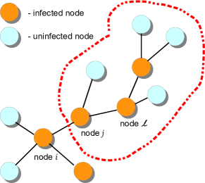
Denote the set of node $i$’s neighbors by ${\cal N}_{i}$. For each $j\in{\cal N}_{i}$, let $C_{j}$ be the size of the infected subcluster including node $j$ after removing the remaining cluster connected to node $j$ by the edge between nodes $i$ and $j$. An example is shown in Fig. 1. In the figure, the infected subcluster containing node $j$ lies inside the dotted red curve. In this example, $C_{j}=3$. When neighbor $j$ is not infected, we set $C_{j}=0$. It is clear that a cascade of infection or contagion happens if and only if $C_{j}=\infty$ for some $j\in{\cal N}_{i}$.

When a neighbor $j$ is infected, the number of $k$-hop neighbors of node $j$ in the aforementioned infected subcluster can be viewed as the size of $k$-th generation in Galton-Watson (G-W) model [17, 42], starting with a single individual: Suppose that node $j$ is infected by node $i$ and that node $\ell$ is a $k$-hop neighbor of node $j$ in the infected subcluster that includes node $j$, for some $k\in{\mathbbm{Z}}_{+}$. When $k=0$, node $\ell$ is node $j$ itself. Let $N$ denote the number of node $\ell$’s infected neighbors that are $k+1$ hops away from node $j$ in the same subcluster and contract the infection from node $\ell$. In the example of Fig. 1, node $\ell$ is one-hop away from node $j$ and the rv $N=1$.

From its construction, the distribution of $N$ does not depend on $k$, and its probability mass function (PMF) ${\bf q}_{N}:{\rm I\kern-2.5ptR}\to[0,1]$ is given by

$${\bf q}_{N}(n)$$

$$= \left\{\begin{array}[]{l}\sum_{d\in\{n+1,\ldots,D_{\max}\}}w^{in}_{d}{{d-1}\choose{n}}\gamma({\bf x})^{n}(1-\gamma({\bf x}))^{d-1-n}\\ \hskip 12.28577pt\mbox{ if }n\in\{0,1,\ldots,D_{\max}-1\},\\ 0\hskip 6.50403pt\mbox{ otherwise},\end{array}\right.$$

where $\gamma({\bf x})$ is the aforementioned probability that the infection of a node is transmitted to a neighbor, and ${\bf w}^{in}=(w_{d}^{in};\ d\in{\mathcal{D}})$ with

$$w_{d}^{in} = \frac{w_{d}(g_{d,P}\ p_{P}^{i}+g_{d,U}\ p_{U}^{i})}{\sum_{d^{\prime}\in{\mathcal{D}}}w_{d^{\prime}}(g_{d^{\prime},P}\ p_{P}^{i}+g_{d^{\prime},U}\ p_{U}^{i})}$$

$$= \frac{\beta_{IA}\cdot w_{d}(g_{d,P}\ p_{P}^{i}+g_{d,U}\ p_{U}^{i})}{\gamma({\bf x})},\ d\in{\mathcal{D}}.$$

Note that, by definition, $w_{d}^{in},\ d\in{\mathcal{D}}$, is the probability that a neighboring node has degree $d$ conditional on it being a victim of a successful indirect attack; the numerator of (III-C) is the probability that a neighbor has a degree $d$ and is vulnerable to infection.

The number of $k$-hop neighbors in the infected subcluster containing node $j$, which we denote by $C_{j}^{k},k\in{\rm I\kern-1.5ptN}$, can now be studied using the G-W model. In Fig. 1, $C_{j}^{k}=1$ for $k\in\{1,2\}$ and $C_{j}^{k}=0$ for $k\geq 3$. Each individual representing an infected node produces $n,\ n\in\{0,1,\ldots,D_{\max}-1\}$, offsprings according to the PMF ${\bf q}_{N}$. Consequently, the probability ${\mathbbm{P}}\left[C_{j}<\infty\right]$ is given by the smallest nonnegative root of the equation $Q_{N}(s)=s$ [17, p. 173], where

$$Q_{N}(s) = \sum_{n\in{\mathbbm{Z}}_{+}}{\bf q}_{N}(n)\ s^{n},\ s\in{\rm I\kern-2.5ptR}\ \mbox{for which the sum}$$

converges.

This solution, denoted by $s^{\star}({\bf x})$, always lies in [0, 1]. Moreover, $s^{\star}({\bf x})=1$ if (i) ${\mathbbm{E}}\left[N\right]<1$ or (ii) ${\mathbbm{E}}\left[N\right]=1$ and $q_{N}(1)\neq 1$. When ${\mathbbm{E}}\left[N\right]>1$, we have $s^{\star}({\bf x})<1$.

By conditioning on the degree of the initial infected node, namely node $i$, we obtain

$${\mathbbm{P}}\left[\mbox{cascade takes place at social state }{\bf x}\right]$$ (18)

$$= 1-\sum_{d\in{\mathcal{D}}}f_{d}\big{(}1-\gamma({\bf x})(1-s^{\star}({\bf x}))\big{)}^{d}.$$

Therefore, assuming $\gamma({\bf x})>0$, ${\mathbbm{E}}\left[N\right]>1$ is a sufficient condition for the cascade probability to be strictly positive. In addition, except for in uninteresting degenerate cases, ${\mathbbm{E}}\left[N\right]>1$ is also a necessary condition. We mention that the task of determining whether a cascade is possible or not can be carried out without explicitly computing the PMF ${\bf q}_{N}$ by noting that ${\mathbbm{E}}\left[N\right]$ is also equal to $\sum_{d\in{\mathcal{D}}}w_{d}^{in}(d-1)\gamma({\bf x})$.

Before we proceed, we summarize questions we are interested in exploring with help of the population game model described in this section:

• Is there a unique NE? If not, what is the structure of NEs?

• What is the relation between the degree of a node and its equilibrium action? How do the parameters $K$ and $\beta_{IA}$, which govern the propagation of infections, influence the choices of different populations at NEs?

• What is the POA/POS? How do the network properties and system parameters affect the POA/POS?

• How do network properties, in particular the node degree distribution and average degree, and system parameters shape the resultant probability of cascade at NEs?

IV Main analytical results

This section aims at providing partial answers to questions Q1 through Q3 based on analytical findings. Before we state our main results, we first state the assumption we impose throughout this and following sections.

Assumption 2

The following inequalities hold.

1. $L_{P}<(1-\xi_{{\rm cov}})\ L_{U}$; and

2. $c_{P}>c_{I}+ded$.
   

Assumption 2-a states that when a player is attacked, its expected cost is smaller when it is protected than when it is insured. This implies that the coverage level is less than 100 percent even when insured. We note that, in addition to deductibles, coinsurance (i.e., $\xi_{{\rm cov}}<1$) is often used to mitigate the issue of moral hazard [23] by sharing risk between both the insurer and the insured. Shetty et al. showed that, in the presence of informational asymmetry, only a portion of damages would be covered by insurance at an equilibrium [39]. Assumption 2-b indicates that the investment a player needs to make in order to protect itself against possible attacks is larger than the insurance premium plus the deductible amount. We believe that these are reasonable assumptions in many cases.

We first examine the structure of NEs of the population games and the effects of parameters $K$ and $\beta_{IA}$ on NEs in Section IV-A. Then, we investigate the social optimum and (an upper bound on) the POA/POS as a function of system parameters in Sections IV-B and IV-C, respectively.

IV-A Population games

Theorem 1

Let ${\bf m}\in{\rm I\kern-2.5ptR}_{+}^{D_{\max}}$ be a population size vector and ${\bf x}^{\star}\in{\mathcal{X}}$ be a corresponding NE for some $K\in{\rm I\kern-1.5ptN}$ and $\beta_{IA}\in(0,1]$. If $x_{d_{1},P}^{\star}>0$ for some $d_{1}\in\{1,2,\ldots,D_{\max}-1\}$, then $x_{d,P}^{\star}=m_{d}$ for all $d>d_{1}$.

The proof of Theorem 1 is similar to that of Theorem 1 in [22] and is omitted.

We note that Theorem 1 also implies the following: If $x_{d_{2},P}^{\star}<m_{d_{2}}$ for some $d_{2}\in\{2,\ldots,D_{\max}\}$, then $x_{d,P}^{\star}=0$ for all $d<d_{2}$.

In practice, the exposure of a node to indirect attacks will depend on many factors, including not only its own degree, but also the degrees and protection levels of its neighbors. Therefore, even the nodes with the same degree may behave differently. However, one would expect that the nodes with larger degrees will likely see higher exposures to indirect attacks and, as a result, have a stronger incentive to invest in protecting themselves against (indirect) attacks. Theorem 1 captures this intuition.

The following theorem suggests that, although an NE may not be unique, the size of each population $d\in{\mathcal{D}}$ investing in protection is identical at all NEs. Its proof follows from a straightforward modification of that of Theorem 2 in [22], and is omitted.

Theorem 2

Suppose that ${\bf x}^{1}$ and ${\bf x}^{2}$ are two NEs of the same population game. Then, $x^{1}_{d,P}=x^{2}_{d,P}$ for all $d\in{\mathcal{D}}$.

The uniqueness of the sizes of protected populations at NEs shown in Theorem 2 is crucial for our study. It implies that the cascade probability, which we adopt as a (global) measure of network security, is identical at all NEs even when there is more than one NE. For this reason, it enables us to examine and compare the network security measured using cascade probabilities, as we vary the node degree distribution and parameters $K$ and $\beta_{IA}$.

Let us explain briefly why an NE is not necessarily unique. Suppose that the expected cost of playing $I$ and $N$ is the same and is smaller than that of playing $P$ for some population $d$ at an NE. Then, there are uncountably many NEs. This is a consequence of an earlier observation that a purchase of insurance by a player does not affect the costs of other players, hence their (optimal) responses.

Because the populations choosing to protect remain the same at all NEs (when more than one NE exist) and the issues of interest to us depend only on populations investing in protection, with a little abuse of notation, we use ${\bf N}({\bf m},K,\beta_{IA})=({\bf N}_{d,a}({\bf m},K,\beta_{IA});\ d\in{\mathcal{D}}\mbox{ and }a\in{\mathcal{A}})$ to denote any arbitrary NE corresponding to a population size vector ${\bf m}$, $K\in{\rm I\kern-1.5ptN}$ and $\beta_{IA}\in(0,1]$, where ${\bf N}_{d,a}({\bf m},K,\beta_{IA})$ is the size of population $d$ playing action $a$ at the NE.

Theorems 1 and 2 state that, for fixed population size vector ${\bf m}$ and parameters $K$ and $\beta_{IA}$, there exists a degree threshold given by

$$\ d^{NE}({\bf m},K,\beta_{IA})=\min\{d\in{\mathcal{D}}\ |\ {\bf N}_{d,P}({\bf m},K,\beta_{IA})>0\}$$

such that only the populations with degree greater than or equal to the threshold would invest in protection at any NE. When the set on the right-hand side (RHS) is empty, we set $d^{NE}({\bf m},K,\beta_{IA})=D_{\max}+1$. The existence of a degree threshold also greatly simplifies the computation of NEs, which are not always easy to compute in general.

The following theorem sheds some light on how the degree threshold $d^{NE}({\bf m},K,\beta_{IA})$ behaves with varying $K$ or $\beta_{IA}$.

Theorem 3

Suppose $K_{1},K_{2}\in{\rm I\kern-1.5ptN}$ with $K_{1}\leq K_{2}$. Then, for any population size vector ${\bf m}$ and IAP $\beta_{IA}\in(0,1]$, we have

$$\sum_{d\in{\mathcal{D}}}{\bf N}_{d,P}({\bf m},K_{1},\beta_{IA})\leq\sum_{d\in{\mathcal{D}}}{\bf N}_{d,P}({\bf m},K_{2},\beta_{IA}).$$

Similarly, for any population size vector ${\bf m}$ and $K\in{\rm I\kern-1.5ptN}$,

$$\sum_{d\in{\mathcal{D}}}{\bf N}_{d,P}({\bf m},K,\beta_{IA}^{1})\leq\sum_{d\in{\mathcal{D}}}{\bf N}_{d,P}({\bf m},K,\beta_{IA}^{2})$$

if $0<\beta_{IA}^{1}\leq\beta_{IA}^{2}\leq 1$.

Proof:

A proof is given in Appendix A. ∎

Theorem 3 is quite intuitive; as $K$ or $\beta_{IA}$ increases, the effect of a successful direct attack is felt by a larger portion of the populations. Consequently, for any fixed social state ${\bf x}$, the exposure $e({\bf x})$ grows with $K$ and $\beta_{IA}$. As a result, some of population that would not invest in protection with smaller $K$ or $\beta_{IA}$ will see greater benefits of protecting themselves because the cost of action $N$ or $I$ increases faster than that of $P$ by Assumption 2. Consequently, a larger fraction of population chooses protection. However, as we will show in Section V-B, these two parameters have very different effects on the resulting cascade probability.

IV-B Social optimum

In this subsection, we consider a scenario where there is a single social player (SP) that makes the decisions for all populations. The goal of the SP is to minimize the overall social cost given as the sum of (i) damages/losses from attacks and (ii) the cost of protection. In other words, the social cost at social state ${\bf x}\in{\mathcal{X}}$ is given by

$$SC({\bf x})$$ (19)

$$= \sum_{d\in{\mathcal{D}}}\Big{[}\Big{(}\sum_{a\in{\mathcal{A}}}x_{d,a}\cdot{\bf C}_{d,a}({\bf x})\Big{)}+x_{d,I}\big{(}Ins({\bf x},d)-c_{I}\big{)}\Big{]}$$

$$= \sum_{d\in{\mathcal{D}}}\Big{(}x_{d,P}\cdot{\bf C}_{d,P}({\bf x})+(m_{d}-x_{d,P}){\bf C}_{d,N}({\bf x})\Big{)}.$$ (20)

Note that $\sum_{d\in{\mathcal{D}}}x_{d,I}\left(Ins({\bf x},d)-c_{I}\right)$ in (19) is the (net) cost for insurer(s). Hence, the social cost given by (19) accounts for the costs of all players, including the insurer(s).

Moreover, it is clear from (20) that the social cost depends only on $x_{d,P},\ d\in{\mathcal{D}}$, as insurance simply shifts some of the risk from the insured to the insurer as pointed out earlier. For this reason, we can limit the possible atomic actions of SP to $\{P,N\}$ and simplify the admissible action space of SP to ${\cal Y}:=\prod_{d\in{\mathcal{D}}}[0,m_{d}]$. An SP action ${\bf y}=\big{(}y_{d};\ d\in{\mathcal{D}}\big{)}\in{\mathcal{Y}}$ specifies the size of each population $d$ that should invest in protection (i.e., $y_{d}$) with an understanding that the remaining population $m_{d}-y_{d}$ plays $N$.

Let us define a mapping ${\bf X}:{\mathcal{Y}}\to{\mathcal{X}}$, where

$${\bf X}_{d,a}({\bf y}) = \left\{\begin{array}[]{cl}y_{d}&\mbox{if }a=P,\\ m_{d}-y_{d}&\mbox{if }a=N,\\ 0&\mbox{if }a=I.\end{array}\right.$$

Fix an SP action ${\bf y}\in{\mathcal{Y}}$. The social cost associated with ${\bf y}$ is given by a mapping $\overline{SC}:{\mathcal{Y}}\to{\rm I\kern-2.5ptR}$, where

$$\overline{SC}({\bf y})=SC\big{(}{\bf X}({\bf y})\big{)}$$

$$=\sum_{d\in{\mathcal{D}}}\Big{(}y_{d}\cdot{\bf C}_{d,P}\big{(}{\bf X}({\bf y})\big{)}+(m_{d}-y_{d}){\bf C}_{d,N}\big{(}{\bf X}({\bf y})\big{)}\Big{)}.$$ (22)

The goal of SP is then to solve the following constrained optimization problem.

SP-OPT:

$$\min_{{\bf y}\in{\mathcal{Y}}}\ \overline{SC}({\bf y})$$ (23)

Let ${\bf y}^{\star}\in\arg\min_{{\bf y}\in{\mathcal{Y}}}\ \overline{SC}({\bf y})$ denote any minimizer of the social cost. When we wish to make the dependence of ${\bf y}^{\star}$ on the population size vector ${\bf m}$, parameter $K$ or IAP $\beta_{IA}$ clear, we shall use ${\bf y}^{\star}({\bf m},K,\beta_{IA})$.

The following theorem reveals that, like NEs, any minimizer ${\bf y}^{\star}$ has a degree threshold so that only the populations with degree greater than or equal to the degree threshold should protect at the social optimum.

Let $d^{\dagger}=\min\{d\in{\mathcal{D}}\ |\ y^{\star}_{d}>0\}$. As before, if the set on the RHS is empty, we set $d^{\dagger}=D_{\max}+1$.

Theorem 4

If $d^{\dagger}<D_{\max}$, $y^{\star}_{d}=m_{d}$ for all $d>d^{\dagger}$.

Proof:

A proof is provided in Appendix B. ∎

We can prove the uniqueness of the minimizer ${\bf y}^{\star}$ by making use of Theorem 4.

Theorem 5

There exists a unique solution ${\bf y}^{\star}({\bf m},K,\beta_{IA})$ to the SP-OPT problem.

Proof:

Please see Appendix C for a proof. ∎

While the statements of Theorems 4 and 5 are similar to those of Theorems 4 and 5 in [22], the proofs in [22] do not apply to the settings in this paper.

The following theorem tells us that the protected population size is never smaller at the social optimum than at an NE. Its proof is similar to that of Theorem 7 in [22] and is omitted.

Theorem 6

Fix a population size vector ${\bf m}$, $K\in{\rm I\kern-1.5ptN}$ and $\beta_{IA}\in(0,1]$. Let ${\bf x}^{\star}={\bf N}({\bf m},K,\beta_{IA})$ and ${\bf y}^{\star}={\bf y}^{\star}({\bf m},K,\beta_{IA})$. Then, $\sum_{d\in{\mathcal{D}}}x^{\star}_{d,P}\leq\sum_{d\in{\mathcal{D}}}y^{\star}_{d}$.

Theorem 6 tells us that the damages/losses due to attacks are higher at NEs than at the system optimum. Hence, because the system optimum is unique, the savings from smaller investments in protection at NEs (compared to system optimum) are outweighed by the increases in damages. Thus, the network security degrades as a result of selfish nature of the players as suggested in [26, 27]. This naturally leads to our next question: How efficient are NEs in comparison to the social optimum?

IV-C Price of anarchy

Inefficiency of NEs is well documented, e.g., [14], [19], [31, Chap. 17-21], [34]. In particular, the Prisoner’s Dilemma illustrates this clearly [33]. However, in some cases, the inefficiency of NEs can be bounded by finite POA/POS [20].

Recall that because all NEs achieve the same social cost in the population games we consider by virtue of Theorem 2, the POA and POS are identical. We are interested in investigating the relation between system parameters, including degree distribution ${{\bf f}}$, $K$ and $\beta_{IA}$, and the POA.

Theorem 7

Let ${\bf m}$ be a population size vector and $d_{{\rm avg}}$ be the average degree of the populations. Suppose $c_{P}\geq\Delta L\cdot\tau_{DA}$. Then, for any $K\in{\rm I\kern-1.5ptN}$ and $\beta_{IA}\in(0,1]$,

$$\frac{SC\big{(}{\bf N}({\bf m},K,\beta_{IA})\big{)}}{\overline{SC}\big{(}{\bf y}^{\star}({\bf m},K,\beta_{IA})\big{)}}\leq 1+d_{{\rm avg}}\cdot e_{\max}({\bf m},K,\beta_{IA}),$$ (24)

where

$$e_{\max}({\bf m},K,\beta_{IA}) = \beta_{IA}\ p_{U}^{i}\sum_{k=0}^{K-1}\left(\frac{\beta_{IA}\ p_{U}^{i}}{d_{{\rm avg}}}\sum_{d\in{\mathcal{D}}}d(d-1)m_{d}\right)^{k}$$

is the largest possible exposure nodes can see when no population invests in protection, i.e., $x_{d,P}=0$ for all $d\in{\mathcal{D}}$.

Proof:

A proof is given in Appendix D. ∎

The assumption $c_{P}\geq\Delta L\cdot\tau_{DA}$ in the theorem is reasonable because it merely requires that the insurance premium is at least the difference in the expected losses sustained only from a direct attack, not including any additional expected losses a player may incur from indirect attacks. Since a private insurer will likely charge a premium high enough to recoup the average insurance payout for insured players, the premium will need to be higher than $\xi_{{\rm cov}}\big{(}\tau_{DA}(1+{d}^{ins}_{{\rm avg}}\cdot e({\bf x}))L_{U}-ded\big{)}$, where $d^{ins}_{{\rm avg}}$ is the average degree of insured players. Therefore, assuming that $\xi_{{\rm cov}}$ is not too small and/or the deductible is not too large, the premium is likely to be at least $\Delta L\cdot\tau_{DA}$.

The upper bound on POA in Theorem 7 is tight in the sense that there are examples where the POA is equal to the bound. We will provide a numerical example in Section V-C, for which the POA is close to our bound in the theorem.

V Numerical results

In this section, we use numerical examples to i) verify our findings in Theorems 1, 3 and 7 and ii) illustrate how cascade probability is shaped by system parameters. For the first three examples in Sections V-A through V-C, we use a family of (truncated) power law degree distributions given by $\big{\{}{\bf m}^{\alpha};\ \alpha\in[0,3]\big{\}}$, where $m^{\alpha}_{d}\propto d^{-\alpha}$, $d\in{\mathcal{D}}$. Over the years, it has been suggested that many of both natural and engineered networks have a power law degree distribution (e.g., [1, 24]). Using Lemma 3 in Appendix D of [22], one can easily show that the degree distribution ${\bf f}({\bf m}^{\alpha})$ becomes smaller in the usual stochastic order [37] with increasing $\alpha$. This implies that the average degree decreases with $\alpha$, which ranges from 1.33 (for $\alpha=3$) to 10.5 (for $\alpha=0$) with $D_{\max}=20$. For the last example in Section V-D, we adopt a family of (truncated) Poisson degree distributions parameterized by $\lambda\in[1.1,10.6]$.

Also, we would like to mention that, although we assume $p_{P}^{i}=0$ and $p_{U}^{i}=1$ for our numerical examples presented here, similar qualitative results hold when other values satisfying $p_{P}^{i}<p_{U}^{i}$ are used.

V-A Cascade probability, degree threshold, and protected population size

The parameter values used in the first example are provided in Table II.

Parameter	Value	Parameter	Value	Parameter	Value
$\tau_{DA}$	0.95	$p_{U}^{i}$	1.0	$p_{P}^{i}$	0
$\xi_{{\rm cov}}$	0.8	$ded$	20	$Cov_{\max}$	500
$L_{P}$	10	$L_{U}$	100	$\beta_{IA}$	0.85
$c_{P}$	300	$c_{I}$	40	$D_{\max}$	20

TABLE II: Parameter values for first numerical example.

(a)                                 (b)

(c)                                 (d)

Figure 2: Plot of (a) degree threshold $d^{NE}({\bf m}^{\alpha},K,\beta_{IA})$, (b) fraction of protected populations, (c) probability of cascade, and (d) ${\mathbbm{E}}\left[N\right]$.

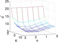
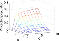
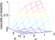
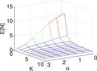
Fig. 2 plots (a) degree threshold $d^{NE}({\bf m}^{\alpha},K,\beta_{IA})$, (b) the fraction of total population that invests in protection at NEs, (c) cascade probability given by (18), and (d) ${\mathbbm{E}}\left[N\right]$ (discussed in Section III-C) as a function of the parameter $K$ and the power law parameter $\alpha$. It is clear from Fig. 2(a) that, with other parameters fixed, the degree threshold $d^{NE}({\bf m}^{\alpha},K,\beta_{IA})$ is nonincreasing in $K$. This leads to a larger fraction of total population investing in protection (Fig. 2(b)) with increasing $K$ as proved in Theorem 3. In addition, Fig. 2(c) shows diminishing cascade probability with increasing $K$.

Fig. 2(b) also suggests that the fraction of protected population in general goes up with an increasing average degree (or, equivalently, decreases with the power law parameter $\alpha$). From this observation, one might expect the cascade probability to diminish with the average degree. Surprisingly, Fig. 2(c) indicates that the cascade probability climbs with an increasing average degree at the same time.

We suspect that this somewhat counterintuitive observation is a consequence of what we see in Fig. 2(a): Over the parameter settings where the cascade probability is nonzero, the degree threshold $d^{NE}({\bf m}^{\alpha},K,\beta_{IA})$ generally rises with the average degree. This suggests that, even though more of the population invests in protection, because nodes with increasing degrees, but smaller than the degree thresholds are still unprotected and vulnerable, it becomes easier for an infection to propagate throughout the network with the help of such vulnerable nodes with increasing degrees.

V-B Effects of indirect attack probability $\beta_{IA}$

In the second example, we vary IAP $\beta_{IA}$ while keeping the values of other parameters the same as in the first example. Our aim is to investigate how the IAP influences the cascade probability and the fraction of protected population and compare it to the effects of parameter $K$.

(a)

(b)

(c)

Figure 3: Plot of the cascade probability and the protected population size. (a) $\alpha=0.2$, (b) $\alpha=1.2$, and (c) $\alpha=2.2$.

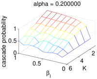
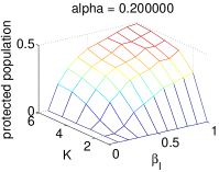
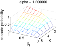
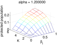
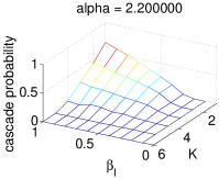
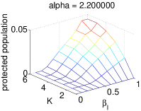
Fig. 3 shows the cascade probability and the fraction of population investing in protection as IAP $\beta_{IA}$ and parameter $K$ are varied for three different values of $\alpha$ ($\alpha=$ 0.2, 1.2 and 2.2).

We point out three observations. First, as alluded to in the first example, the cascade probability decreases with $\alpha$, as does the fraction of protected population. As mentioned in Section II, this observation is in sharp contrast with the findings by Watts [44]. Figs. 2 and 3 suggest that when the nodes are strategic and can choose to protect themselves to reduce the probability of infection, at least for certain parameter regimes, the network becomes less stable in that the cascade probability rises as the average degree increases (i.e., $\alpha$ decreases) and the second (phase) transition observed in [44] and described in Section II is missing.

Second, it is clear from Fig. 3 that, although a larger fraction of population invests in protection with increasing $\beta_{IA}$ as proved in Theorem 3, the cascade probability also rises. What may be surprising at first sight is how differently the parameters $K$ and $\beta_{IA}$ affect cascade probability in spite of the similarity in the way they influence the portion of protected populations as illustrated in Fig. 3; while raising $K$ results in diminished cascade probability, increasing $\beta_{IA}$ leads to rising cascade probability.

This can be explained as follows: Once other parameters and social state are fixed, cascade probability does not depend on $K$. Hence, increasing the protected population size reduces cascade probability. On the other hand, with other parameters and social state fixed, cascade probability climbs with $\beta_{IA}$. Thus, although the fraction of protected population increases with $\beta_{IA}$, because the nodes are strategic, they do not invest enough in protection to keep cascade probability from rising. This can be partially inferred from growing inefficiency of NEs as hinted by the upper bound on POA in Theorem 7.

Third, Fig. 3 indicates that the effect of IAP is more pronounced when the average degree is larger in the sense that cascade probability rises more quickly with the IAP (when it is small). This is intuitive; when the network is highly connected, it provides an infection with a greater number of paths through which the infection can spread. Hence, even when the IAP is relatively small, it will be able to propagate throughout the network more easily.

V-C Price of anarchy

In the next example, we examine the POA as the average degree of nodes varies. We set $K=5$ for this example. The values of other parameters are listed in Table III. For this example, we purposely choose parameter values so that the POA is close to its upper bound.

Parameter	Value	Parameter	Value	Parameter	Value
$\tau_{DA}$	0.9	$p_{U}^{i}$	1.0	$p_{P}^{i}$	0
$\xi_{{\rm cov}}$	0.95	$ded$	5	$Cov_{\max}$	500
$L_{P}$	5	$L_{U}$	95	$\beta_{IA}$	0.1
$c_{P}$	88	$c_{I}$	80	$D_{\max}$	20

TABLE III: Parameter values for first numerical example.

Fig. 4 plots (a) degree threshold $d^{NE}({\bf m}^{\alpha},5,0.1)$, (b) fraction of protected population, and (c) POA and its bound in Theorem 7. We change the $x$-axis to average degree so that it is easier to see the effect of average degree on the realized POA and the bound. Recall that the average degree decreases with increasing $\alpha$.

(a)                      (b)                     (c)

Figure 4: Plot of (a) degree thresholds, (b) fraction of protected population, and (c) POA.

First, it is obvious from Fig. 4(c) that both the POA and the bound grow much faster than linearly. Hence, while a greater portion of populations elects to protect when $\alpha$ is smaller (hence, the average degree is larger) as shown in previous subsections, the cascade probability rises with an increasing average degree, and so does the POA. These findings suggest that when the nodes are strategic entities interested only in minimizing their own costs, for keeping the cascade probability small, it is better to have less evenly distributed node degrees with fewer large-degree nodes.

Second, Figs. 4(b) and 4(c) tell us the following interesting story. When $\alpha$ is small (i.e., the degree distribution is more even), although nodes with degrees less than five, which account for about 20-30 percent of total population, do not invest in protection at the system optimum, the POA closely tracks the bound and rises rapidly with the average degree. Therefore, there is an interesting trade-off one can observe: When the degree distribution is less evenly distribution, the network is held together by nodes with high degrees. Such networks are shown to be robust against random attacks, but are more vulnerable to coordinated attacks targeting high-degree nodes [10, 11]. One possible way to mitigate the vulnerability is to increase the connectivity of the network, hence, the average degree. However, Fig. 4(a) indicates that increasing network connectivity not only leads to higher cascade probability as illustrated in previous subsections, but also results in a higher social cost and greater POA, which is undesirable.

V-D Poisson degree distribution

In the last example, we consider a family of (truncated) Poisson degree distribution $\big{\{}{\bf m}^{\lambda};\ \lambda\in[1.1,10.6]\big{\}}$, where $m^{\lambda}_{d}\propto\lambda^{d}/d!,\ d\in{\mathcal{D}}$. The remaining parameters are identical to those in Table II of Section V-A.

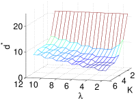
(a)                                 (b)

Figure 5: Plot of (a) degree threshold $d^{NE}({\bf m}^{\lambda},K,\beta_{IA})$, and (b) fraction of protected populations.

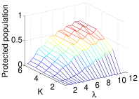
Fig. 5 shows (a) the degree threshold $d^{NE}({\bf m}^{\lambda},K,\beta_{IA})$ and (b) the fraction of protected populations as a function of $\lambda$ and $K$. Clearly, the percentage of protected population tends to increase with the average degree (although there is no strict monotonicity), which is consistent with an earlier observation with power law degree distributions. In addition, the degree threshold $d^{NE}({\bf m}^{\lambda},K,\beta_{IA})$ tends to climb with the average degree.

(a)                                 (b)

Figure 6: Plot of cascade probability. (a) Poisson distributions, (b) power laws.

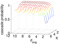
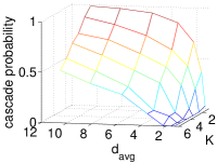
In Fig. 6, we plot the cascade probability for both (a) Poisson distributions and (b) power laws. There are two observations we would like to point out. First, in the case of Poisson distributions, the cascade probability shows a cyclic behavior. While similar cyclic patterns exist with power law degree distributions as well, they are more pronounced with Poisson degree distributions. These cycles shown in Fig. 6(a) coincide with the degree threshold $d^{NE}({\bf m}^{\lambda},K,\beta_{IA})$ in Fig. 5(a); the dips in the cascade probability occur while the degree threshold remains constant. We suspect that these cycles are a side effect of a population game model that is a deterministic model. Nonetheless, the two plots show similar general trends and the cascade probability reveals an increasing trend with the average degree for both power law and Poisson degree distributions.

Second, the cascade probability exhibits higher sensitivity with respect to the average degree, especially when the average degree is small, in case of Poisson distributions. In other words, as the average degree rises, the cascade probability increases more rapidly with Poisson distributions than with power laws. This suggests that, even for a fixed average degree, the cascade probability is likely to depend very much on the underlying degree distribution.

VI Conclusions

We studied interdependent security with strategic agents. In particular, we examined how various system parameters and network properties shape the decisions of strategic agents and resulting system security and social cost. We established the existence of a degree threshold at both Nash equilibria and social optima. Furthermore, we demonstrated the uniqueness of social cost at Nash equilibria, although there could be more than one Nash equilibrium. In addition, we derived an upper bound on the POA, which increases superlinearly with the average degree of nodes in general, and demonstrated that the bound is tight. Finally, our study suggests that as the average degree increases, despite a higher fraction of nodes investing in protection at Nash equilibria, cascade probability also rises.

Appendix A Proof of Theorem 3

We only prove the first part of the theorem as the second part follows from essentially an identical argument. Suppose that the theorem is false for some population size vector ${\bf m}$, IAP $\beta_{IA}$, and two distinct $K_{1}$ and $K_{2}$ satisfying $1\leq K_{1}<K_{2}$. We will show that this results in a contradiction. In order to make the dependence on the parameter $K$ explicit, we denote the cost function ${\bf C}({\bf x})$ and the exposure $e({\bf x})$ by ${\bf C}({\bf x};K)$ and $e({\bf x};K)$, respectively. Moreover, for notational simplicity, we denote ${\bf N}({\bf m},K_{i},\beta_{IA}),\ i=1,2,$ by ${\bf x}^{i}$ in this section.

We first state a property that will be used shortly.

Property P1: Suppose that $\bar{{\bf x}}^{1}$ and $\bar{{\bf x}}^{2}$ are two social states such that $e(\bar{{\bf x}}^{1})<e(\bar{{\bf x}}^{2})$. Then, the following inequalities hold, which follow directly from the cost function given in (3) - (14) and Assumption 2-a: For all $d\in{\mathcal{D}}$,

$$0<{\bf C}_{d,P}(\bar{{\bf x}}^{2})-{\bf C}_{d,P}(\bar{{\bf x}}^{1}) < {\bf C}_{d,I}(\bar{{\bf x}}^{2})-{\bf C}_{d,I}(\bar{{\bf x}}^{1})$$

$$\leq {\bf C}_{d,N}(\bar{{\bf x}}^{2})-{\bf C}_{d,N}(\bar{{\bf x}}^{1}).$$

We point out that this property continues to hold even when we compare social states for two different population sizes ${\bf m}^{1}$ and ${\bf m}^{2}$ or for different values of parameter $K$ or $\beta_{IA}$, which satisfy the inequality in the exposures.

Let $d_{i}=\min\{d\in{\mathcal{D}}\ |\ x^{i}_{d,P}>0\}$, $i=1,2$, with an understanding $d_{i}=D_{\max}+1$ if $x^{i}_{d,P}=0$ for all $d\in{\mathcal{D}}$. Then, from the above assumption and Theorem 1, we must have $x_{d_{1},P}^{2}<x_{d_{1},P}^{1}$. By the definition of an NE,

$${\bf C}_{d_{1},P}({\bf x}^{1};K_{1})\leq\min\{{\bf C}_{d_{1},I}({\bf x}^{1};K_{1}),\ {\bf C}_{d_{1},N}({\bf x}^{1};K_{1})\}.$$ (25)

From the assumption $x_{d,P}^{2}\leq x_{d,P}^{1}$ for all $d\in{\mathcal{D}}$ and $x_{d_{1},P}^{2}<x_{d_{1},P}^{1}$, we get $e({\bf x}^{1};K_{1})<e({\bf x}^{2};K_{2})$. Therefore, property P1 tells us

$${\bf C}_{d_{1},P}({\bf x}^{2};K_{2})-{\bf C}_{d_{1},P}({\bf x}^{1};K_{1})$$ (26)

$$< \min_{a\in\{N,I\}}\big{(}{\bf C}_{d_{1},a}({\bf x}^{2};K_{2})-{\bf C}_{d_{1},a}({\bf x}^{1};K_{1})\big{)}.$$

Together with (25), the inequality in (26) yields

$${\bf C}_{d_{1},P}({\bf x}^{2};K_{2})<\min\{{\bf C}_{d_{1},N}({\bf x}^{2};K_{2}),\ {\bf C}_{d_{1},I}({\bf x}^{2};K_{2})\}.$$

Obviously, this implies $x_{d_{1},P}^{2}=m_{d_{1}}$ and, hence, contradicts the assumption $x_{d_{1},P}^{2}<x_{d_{1},P}^{1}\leq m_{d_{1}}$.

Appendix B Proof of Theorem 4

We prove the theorem by contradiction. Assume that there exists $d^{\prime}>d^{\dagger}$ such that $y_{d^{\prime}}^{\star}<m_{d^{\prime}}$. Suppose that $\epsilon$ is a constant satisfying $0<\epsilon<\min\{y_{d^{\dagger}}^{\star},\ m_{d^{\prime}}-y_{d^{\prime}}^{\star}\}$ and ${\bf u}_{d}$ is a zero-one vector whose only non-zero element is the $d$-th entry. Let ${\bf y}^{\dagger}={\bf y}^{\star}+\epsilon\big{(}{\bf u}_{d^{\prime}}-{\bf u}_{d^{\dagger}}\big{)}$. We will show that $\overline{SC}({\bf y}^{\dagger})<\overline{SC}({\bf y}^{\star})$, contradicting the assumption that ${\bf y}^{\star}$ is a minimizer of the social cost. For notational simplicity, we write ${\bf x}^{\dagger}$ and ${\bf x}^{\star}$ in place of ${\bf X}({\bf y}^{\dagger})$ and ${\bf X}({\bf y}^{\star})$, respectively, throughout this section.

After a little algebra,

$$\overline{SC}({\bf y}^{\star})-\overline{SC}({\bf y}^{\dagger})$$ (27)

$$= \tau_{DA}\left(e({\bf x}^{\star})-e({\bf x}^{\dagger})\right)\sum_{d\in{\mathcal{D}}}d\left(y_{d}^{\star}\ L_{P}+(m_{d}-y_{d}^{\star})L_{U}\right)$$

$$+\ \epsilon\ \tau_{DA}(d^{\prime}-d^{\dagger})e({\bf x}^{\dagger})\Delta L.$$

It is clear that the second term in (27) is strictly positive because $d^{\prime}>d^{\dagger}$, $e({\bf x}^{\dagger})>0$ and $\Delta L>0$. Thus, to show that (27) is nonnegative, it suffices to prove $e({\bf x}^{\dagger})<e({\bf x}^{\star})$. To this end, we demonstrate $\gamma({\bf x}^{\dagger})<\gamma({\bf x}^{\star})$ and $\lambda({\bf x}^{\dagger})<\lambda({\bf x}^{\star})$. From (6), these inequalities imply $e({\bf x}^{\dagger})<e({\bf x}^{\star})$.

First, from (3),

$$\gamma({\bf x}^{\star})-\gamma({\bf x}^{\dagger}) = \frac{\epsilon\ \beta_{IA}\ \Delta p}{d_{{\rm avg}}}\left(d^{\prime}-d^{\dagger}\right)>0.$$

Second, from (5), we get

$$\lambda({\bf x}^{\star})-\lambda({\bf x}^{\dagger}) = \frac{\epsilon\ \beta_{IA}\ \Delta p}{d_{{\rm avg}}}\big{(}d^{\prime}(d^{\prime}-1)-d^{\dagger}(d^{\dagger}-1)\big{)}>0.$$

Appendix C Proof of Theorem 5

Suppose that the theorem is not true and there exist two distinct minimizers ${\bf y}^{1}$ and ${\bf y}^{2}$. By Theorem 4, without loss of generality, we assume i) $y_{d}^{1}\leq y_{d}^{2}$ for all $d\in{\mathcal{D}}$ and ii) $y_{d}^{1}<y_{d}^{2}$ for at least one $d\in{\mathcal{D}}$. We will show that this leads to a contradiction. Throughout this section, we denote ${\bf X}({\bf y}^{i}),\ i=1,2,$ by ${\bf x}^{i}$ for notational simplicity.

Let $d^{i}=\min\{d\in{\mathcal{D}}\ |\ y^{i}_{d}>0\},\ i=1,2,$ with the convention $d^{i}=D_{\max}+1$ if ${\bf y}^{i}={\bf 0}$. Note that $d^{2}\leq D_{\max}$ by assumption. Since $y^{2}_{d^{2}}>0$, with a little abuse of notation, the one-sided partial derivative of the social cost with respect to $y_{d^{2}}$ at ${\bf y}^{2}$ satisfies

$$\frac{\partial}{\partial y_{d^{2}}}\overline{SC}({\bf y}^{2}):=\lim_{\delta\downarrow 0}\frac{\overline{SC}({\bf y}^{2})-\overline{SC}({\bf y}^{2}-\delta\cdot{\bf u}_{d^{2}})}{\delta}\leq 0$$

with the equality holding when $y^{2}_{d^{2}}<m_{d^{2}}$. Define another one-sided partial derivative of the social cost with respect to $y_{d^{2}}$ at ${\bf y}^{1}$ to be

$$\frac{\partial}{\partial y_{d^{2}}}\overline{SC}({\bf y}^{1}):=\lim_{\delta\downarrow 0}\frac{\overline{SC}({\bf y}^{1}+\delta\cdot{\bf u}_{d^{2}}))-\overline{SC}({\bf y}^{1})}{\delta}.$$

Since ${\bf y}^{1}$ minimizes the social cost, $\partial\overline{SC}({\bf y}^{1})/\partial y_{d^{2}}\geq 0$. However, we will show that $\partial\overline{SC}({\bf y}^{1})/\partial y_{d^{2}}<\partial\overline{SC}({\bf y}^{2})/\partial y_{d^{2}}\leq 0$, leading to a contradiction.

From (22),

$$\frac{\partial}{\partial y_{d^{2}}}\overline{SC}({\bf y}^{i})={\bf C}_{d^{2},P}({\bf x}^{i})-{\bf C}_{d^{2},N}({\bf x}^{i})$$ (28)

$$+\sum_{d\in{\mathcal{D}}}\left(y_{d}^{i}\frac{\partial}{\partial y_{d^{2}}}{\bf C}_{d,P}({\bf x}^{i})+(m_{d}-y_{d}^{i})\frac{\partial}{\partial y_{d^{2}}}{\bf C}_{d,N}({\bf x}^{i})\right).$$

Using the cost function in (13), we obtain

$$\frac{\partial}{\partial y_{d^{2}}}{\bf C}_{d,P}({\bf x}^{i}) = \tau_{DA}\ L_{P}\ d\frac{\partial}{\partial y_{d^{2}}}e({\bf x}^{i}),\mbox{ and }$$

$$\frac{\partial}{\partial y_{d^{2}}}{\bf C}_{d,N}({\bf x}^{i}) = \tau_{DA}\ L_{U}\ d\frac{\partial}{\partial y_{d^{2}}}e({\bf x}^{i}).$$

Here, $\partial e({\bf x}^{i})/\partial y_{d^{2}}$ and $\partial{\bf C}_{d,a}({\bf x}^{i})/\partial y_{d^{2}}$, $a\in\{P,N\}$, are appropriate one-sided partial derivatives. Substituting these in (28),

$$\frac{\partial}{\partial y_{d^{2}}}\overline{SC}({\bf y}^{i})=c_{P}-\tau_{DA}\left(1+d^{2}\ e({\bf x}^{i})\right)\Delta L$$ (29)

$$+\sum_{d\in{\mathcal{D}}}\tau_{DA}\ d\left(y_{d}^{i}\ L_{P}+(m_{d}-y_{d}^{i})L_{U}\right)\frac{\partial}{\partial y_{d^{2}}}e({\bf x}^{i}).$$

We rewrite $\partial\overline{SC}({\bf y}^{1})/\partial y_{d^{2}}$ in a more convenient form for our purpose.

$$\frac{\partial}{\partial y_{d^{2}}}\overline{SC}({\bf y}^{1})=c_{P}-\tau_{DA}\left(1+d^{2}\ e({\bf x}^{1})\right)\Delta L$$

$$+\sum_{d\in{\mathcal{D}}}\tau_{DA}\ d\left(y_{d}^{2}\ L_{P}+(m_{d}-y_{d}^{2})L_{U}+(y_{d}^{2}-y_{d}^{1})\Delta L\right)$$

$$\hskip 50.58878pt\times\frac{\partial}{\partial y_{d^{2}}}e({\bf x}^{1})$$

Using the above expression,

$$\frac{\partial}{\partial y_{d^{2}}}\overline{SC}({\bf y}^{2})-\frac{\partial}{\partial y_{d^{2}}}\overline{SC}({\bf y}^{1})$$

$$= \tau_{DA}\ d^{2}\ \Delta L\big{(}e({\bf x}^{1})-e({\bf x}^{2})\big{)}$$

$$-\sum_{d\in{\mathcal{D}}}\tau_{DA}\ d\Big{[}\left(y_{d}^{2}\ L_{P}+(m_{d}-y_{d}^{2})L_{U}\right)$$

$$\hskip 50.58878pt\times\left(\frac{\partial}{\partial y_{d^{2}}}e({\bf x}^{1})-\frac{\partial}{\partial y_{d^{2}}}e({\bf x}^{2})\right)$$

$$\hskip 50.58878pt+(y_{d}^{2}-y_{d}^{1})\Delta L\frac{\partial}{\partial y_{d^{2}}}e({\bf x}^{1})\Big{]}.$$

Because ${\bf y}^{1}\leq{\bf y}^{2}$, where the inequality is element-wise, and $y_{d^{2}}^{2}>y_{d^{2}}^{1}$, we have $e({\bf x}^{2})<e({\bf x}^{1})$ and the first term in (C) is positive. Moreover, from the definition of the exposure in (6), it is clear $\partial e({\bf x}^{1})/\partial y_{d^{2}}<0$. Thus, in order to prove $(\ref{eq:appen5a-3})>0$, it suffices to show $\partial e({\bf x}^{1})/\partial y_{d^{2}}<\partial e({\bf x}^{2})/\partial y_{d^{2}}$.

$$\frac{\partial}{\partial y_{d^{2}}}e({\bf x}^{i})$$

$$= \left(\frac{\partial}{\partial y_{d^{2}}}\gamma({\bf x}^{i})\right)\sum_{k=0}^{K-1}\lambda({\bf x}^{i})^{k}+\gamma({\bf x}^{i})\sum_{k=0}^{K-1}\frac{\partial}{\partial y_{d^{2}}}\lambda({\bf x}^{i})^{k}$$

$$= -\frac{\beta_{IA}\ \Delta p\ d^{2}}{d_{{\rm avg}}}\left[\sum_{k=0}^{K-1}\lambda({\bf x}^{i})^{k}\right.$$

$$\hskip 50.58878pt\left.+\gamma({\bf x}^{i})(d^{2}-1)\sum_{k=1}^{K-1}k\ \lambda({\bf x}^{i})^{k-1}\right].$$

As $\gamma({\bf x}^{2})<\gamma({\bf x}^{1})$ and $\lambda({\bf x}^{2})<\lambda({\bf x}^{1})$, we have from (C) the desired inequality $\partial e({\bf x}^{1})/\partial y_{d^{2}}<\partial e({\bf x}^{2})/\partial y_{d^{2}}$.

Appendix D Proof of Theorem 7

Let ${\bf x}^{\star}={\bf N}({\bf m},K,\beta_{IA})$ be an NE and ${\bf y}^{\star}={\bf y}^{\star}({\bf m},K,\beta_{IA})$ for notational convenience. Also, we write $e({\bf y}^{\star})$ in place of $e({\bf X}({\bf y}^{\star}))$. By slightly rewriting the social costs given by (20) and (22), we obtain

$$\overline{SC}({\bf y}^{\star}) = (c_{P}-\Delta L\ \tau_{DA})\sum_{d\in{\mathcal{D}}}y_{d}^{\star}+\tau_{DA}\ L_{U}$$

$$+\tau_{DA}\ L_{U}\ d_{{\rm avg}}\ e({\bf y}^{\star})-\Delta L\ \tau_{DA}\ e({\bf y}^{\star})\sum_{d\in{\mathcal{D}}}d\cdot y_{d}^{\star}$$

and

$$SC({\bf x}^{\star}) = \big{(}c_{P}-\Delta L\ \tau_{DA}\big{)}\sum_{d\in{\mathcal{D}}}x_{d,P}^{\star}+\tau_{DA}\ L_{U}$$

$$+\tau_{DA}\ L_{U}\ d_{{\rm avg}}\ e({\bf x}^{\star})-\Delta L\ \tau_{DA}\ e({\bf x}^{\star})\sum_{d\in{\mathcal{D}}}d\cdot x_{d,P}^{\star}.$$

We first derive an upper bound on the difference $SC({\bf x}^{\star})-\overline{SC}({\bf y}^{\star})$ followed by a lower bound on $\overline{SC}({\bf y}^{\star})$.

Subtracting $\overline{SC}({\bf y}^{\star})$ from $SC({\bf x}^{\star})$,

$$SC({\bf x}^{\star})-\overline{SC}({\bf y}^{\star})$$

$$= \big{(}c_{P}-\Delta L\ \tau_{DA}\big{)}\Big{(}\sum_{d\in{\mathcal{D}}}x_{d,P}^{\star}-\sum_{d\in{\mathcal{D}}}y_{d}^{\star}\Big{)}$$

$$+\Delta L\ \tau_{DA}\Big{(}e({\bf y}^{\star})\sum_{d\in{\mathcal{D}}}(y_{d}^{\star}\cdot d)-e({\bf x}^{\star})\sum_{d\in{\mathcal{D}}}(x_{d,P}^{\star}\cdot d)\Big{)}$$

$$+\tau_{DA}\ L_{U}\ d_{{\rm avg}}\big{(}e({\bf x}^{\star})-e({\bf y}^{\star})\big{)}.$$

From Theorems 2, 4 and 6, we know $x^{\star}_{d,P}\leq y^{\star}_{d}$. Hence, together with the assumption $c_{P}\geq\Delta L\ \tau_{DA}$, we get

$$SC({\bf x}^{\star})-\overline{SC}({\bf y}^{\star})$$ (32)

$$\leq \Delta L\ \tau_{DA}\Big{(}e({\bf y}^{\star})\sum_{d\in{\mathcal{D}}}(y_{d}^{\star}\cdot d)-e({\bf x}^{\star})\sum_{d\in{\mathcal{D}}}(x_{d,P}^{\star}\cdot d)\Big{)}$$

$$+\tau_{DA}\ L_{U}\ d_{{\rm avg}}\big{(}e({\bf x}^{\star})-e({\bf y}^{\star})\big{)}.$$

We consider the following two cases.

Case 1: $e({\bf y}^{\star})\sum_{d\in{\mathcal{D}}}(y_{d}^{\star}\cdot d)\geq e({\bf x}^{\star})\sum_{d\in{\mathcal{D}}}(x_{d,P}^{\star}\cdot d)$ – In this case, we have

$$(\ref{eq:appen8-0}) \leq L_{U}\ \tau_{DA}\Big{(}e({\bf y}^{\star})\sum_{d\in{\mathcal{D}}}(y_{d}^{\star}\cdot d)-e({\bf x}^{\star})\sum_{d\in{\mathcal{D}}}(x_{d,P}^{\star}\cdot d)\Big{)}$$ (33)

$$+\tau_{DA}\ L_{U}\ d_{{\rm avg}}\big{(}e({\bf x}^{\star})-e({\bf y}^{\star})\big{)}$$

$$= L_{U}\ \tau_{DA}\Big{[}e({\bf x}^{\star})\Big{(}d_{{\rm avg}}-\sum_{d\in{\mathcal{D}}}(x_{d,P}^{\star}\cdot d)\Big{)}$$

$$\hskip 28.90755pt-e({\bf y}^{\star})\Big{(}d_{{\rm avg}}-\sum_{d\in{\mathcal{D}}}(y_{d}^{\star}\cdot d)\Big{)}\Big{]}.$$

From (33) it is clear that the maximum is achieved when ${\bf x}^{\star}={\bf 0}$ and ${\bf y}^{\star}={\bf m}$. Hence,

$$(\ref{eq:appen8-0}) \leq \tau_{DA}\ L_{U}\ d_{{\rm avg}}\ e_{\max}({\bf m},K,\beta_{IA}).$$

Case 2: $e({\bf y}^{\star})\sum_{d\in{\mathcal{D}}}(y_{d}^{\star}\cdot d)<e({\bf x}^{\star})\sum_{d\in{\mathcal{D}}}(x_{d,P}^{\star}\cdot d)$ – Under the assumption, it is obvious

$$(\ref{eq:appen8-0}) \leq \tau_{DA}\ L_{U}\ d_{{\rm avg}}\big{(}e({\bf x}^{\star})-e({\bf y}^{\star})\big{)}$$

$$\leq \tau_{DA}\ L_{U}\ d_{{\rm avg}}\ e_{\max}({\bf m},K,\beta_{IA}).$$

From these two cases, it is clear that $\tau_{DA}\ L_{U}\ d_{{\rm avg}}\ e_{\max}({\bf m},K,\beta_{IA})$ is an upper bound for $SC({\bf x}^{\star})-\overline{SC}({\bf y}^{\star})$.

Since we assume $c_{P}\geq\Delta L\ \tau_{DA}$, we get the following lower bound on $\overline{SC}({\bf y}^{\star})$.

$$\overline{SC}({\bf y}^{\star}) \geq \tau_{DA}\ L_{U}+\tau_{DA}\ e({\bf y}^{\star})\big{(}L_{U}\cdot d_{{\rm avg}}-\Delta L\sum_{d\in{\mathcal{D}}}d\cdot y_{d}^{\star}\big{)}$$

$$\geq \tau_{DA}\ L_{U},$$

where the second inequality is a consequence of $L_{U}\cdot d_{{\rm avg}}\geq\Delta L\sum_{d\in{\mathcal{D}}}d\cdot y_{d}^{\star}$.

Using the above upper bound on $SC({\bf x}^{\star})-\overline{SC}({\bf y}^{\star})$ and the lower bound on $\overline{SC}({\bf y}^{\star})$,

$$\frac{SC({\bf x}^{\star})}{\overline{SC}({\bf y}^{\star})} = 1+\frac{SC({\bf x}^{\star})-\overline{SC}({\bf y}^{\star})}{\overline{SC}({\bf y}^{\star})}$$

$$\leq 1+\frac{\tau_{DA}\ L_{U}\ d_{{\rm avg}}\ e_{\max}({\bf m},K,\beta_{IA})}{\tau_{DA}\ L_{U}}$$

$$= 1+d_{{\rm avg}}\ e_{\max}({\bf m},K,\beta_{IA}).$$

References

- [1] R. Albert, H. Jeong and A.-L. Barabsi, “Error and attack tolerance of complex networks,” Nature, 406:378-382, Jul. 2000.
- [2] N. Beale, D.G. Rand, H. Battey, K. Croxson, R.M. May and M.A. Nowak, “Individual versus systemic risk and the regulator’s dilemma,” Proceedings of the National Academy of Sciences of the United States of America (PNAS), 108(31):12647-12652, Aug. 2011.
- [3] L. Bilge and T. Dumitras, “Before we knew it: an empirical study of zero-day attacks in the real world,” Proc. of ACM Conference on Computer and Communications Security (CCS), Oct. 2012.
- [4] J.C. Bolot and M. Lelarge, “A new perspective on Internet security using insurance,” Proc. of IEEE INFOCOM, Phoenix (AZ), Apr. 2008.
- [5] C.D. Brummitt, K.-M. Lee and K.-I. Goh, “Multiplexity-facilitated cascades in networks,” Physical Review E, 85, 045102(R), 2012.
- [6] F. Caccioli, T.A. Catanach, and J.D. Farmer, “Heterogeneity, correlations and financial contagion,” arXiv:1109.1213, Sep. 2011.
- [7] F. Caccioli, T.A. Catanach, and J.D. Farmer, “Stability analysis of financial contagion due to overlapping portfolios,” arXiv:1210.5987, Oct. 2012.
- [8] D.S. Callaway, M.E.J. Newman, S.H. Strogatz and D.J. Watts, “Network robustness and fragility: percolation and random graphs,” Physical Review Letters, 85(25):5468-5471, Dec. 2000.
- [9] F. Chung and L. Lu, “Connected components in random graphs with given expected degree sequences,” Annals of Combinatorics, 6(2):125-145, Nov. 2002.
- [10] R. Cohen, K. Erez, D. ben-Avraham and S. Havlin, “Resilience of the Internet to random breakdowns,” Physical Review Letters, 85(21):4626-4628, Nov. 2000.
- [11] R. Cohen, K. Erez, D. ben-Avraham and S. Havlin, “Breakdown of the Internet under intentional attack,” Physical Review Letters, 86(16):3682-3685, Apr. 2001.
- [12] E. Coupechoux and M. Lelarge, “Impact of clustering on diffusions and contagions in random networks,” Proc. of Network Games, Control and Optimization (NetGCoop), Paris (France), Oct. 2011.
- [13] E. Coupechoux and M. Lelarge, “How clustering affects epidemics in random networks,”’ Advances in Applied Probability, 46(4):985-1008.
- [14] P. Dubey, “Inefficiency of Nash equilibria,” Mathematics of Operations Research, 11(1):1-8, Feb. 1986.
- [15] P. Gai and S. Kapadia, “Contagion in financial networks,” Proceedings of the Royal Society A, 466:2401-2423, 2010.
- [16] J.P. Gleeson and D.J. Cahalane, “Seed size strongly affects cascades on random networks,” Physical Review E, 75, 056103, 2007.
- [17] G. Grimmett and D. Stirzaker, Probability and Random Processes, third ed., Oxford University Press, 2001.
- [18] G. Heal and H. Kunreuther, “Interdependent security: a general model,” National Bureau of Economic Research (NBER) Working Paper No. 10706, Aug. 2004.
- [19] R. Johari and J.N. Tsitsiklis, “Efficiency loss in a network resource allocation game,” Mathematics of Operations Research, 29(3):407-435, Aug. 2004.
- [20] E. Koutsoupias and C.H. Papadimitriou, “Worst-case equilibria,” Proc. of the 16th Annual Symposium on Theoretical Aspects of Computer Science (STACS), pp. 404-413, 1999.
- [21] H. Kunreuther and G. Heal, “Interdependent Security,” The Journal of Risk and Uncertainty, 26(2/3):231-249, 2003.
- [22] R.J. La, “Effects of degree distributions on network security – population game model,” IEEE/ACM Trans. of Networking, under review. Available at http://www.ece.umd.edu/hyongla/PAPERS/La_TON_IDS_Local.pdf.
- [23] J.-J. Laffont and D. Martimort, The Theory of Incentives: The Principal-Agent Model, Princeton University Press, 2001.
- [24] A. Lakhina, J. Byers, M. Crovella and P. Xi, “Sampling biases in IP topology measurements,”’ Proc. of IEEE INFOCOM, San Francisco (CA), Apr. 2003.
- [25] A. Laszka, M. Felegyhazi and L. Buttyn, “A survey of interdependent security games,” CrySys Lab Technical Report No. CRYSYS-TR-2012-11-15.
- [26] M. Lelarge and J. Bolot, “A local mean field analysis of security investments in networks,” Proc. of the 3rd International Workshop on Economics of Networked Systems (NetEcon), pp. 25-30, Seattle (WA), Aug. 2008.
- [27] M. Lelarge and J. Bolot, “Economic incentives to increase security in the Internet: the case for insurance,” Proc. of IEEE INFOCOM, Rio de Janeiro (Brazil), Apr. 2009.
- [28] A. Melnikov, Risk Analysis in Finance and Insurance, 2nd ed., CRC Press, 2011.
- [29] M. Molloy and B. Reed, “A critical point for random graphs with a given degree sequence,” Random Structures and Algorithms, 6:161-180, 1995.
- [30] M. Molloy and B. Reed. “The size of the largest component of a random graph on a fixed degree sequence,” Combinatorics, Probability and Computing, 7(3):295-305, Sep. 1998.
- [31] N. Nisan, T. Roughgarden, . Tardos, and V.V. Vazirani, Algorithmic Game Theory, Cambridge University Press, 2007.
- [32] S. Pal and A.M. Makowski, “Sampling random graphs with arbitrary degree distributions,”’ Preprint, 2013.
- [33] W. Poundstone, Prisoner’s Dilemma, Anchor, 1993.
- [34] T. Roughgarden, Selfish Routing and the Price of Anarchy, The MIT Press, 2005.
- [35] W.H. Sandholm Population Games and Evolutionary Dynamics, The MIT Press, 2010.
- [36] C. Seshadhri, T.G. Kolda and A. Pinar, “Community structure and scale-free collections of Erds-Rnyi graphs,” Physical Review E, 85,056109, 2012.
- [37] M. Shaked and J.G. Shanthikumar, Stochastic Orders, Springer Series in Statistics, Springer, 2007.
- [38] C. Shapiro and H.R. Varian, Information Rules, Harvard Business School Press, 1999.
- [39] N. Shetty, G. Schwartz, M. Felegyhazi and J. Walrand, “Competitive cyber-insurance and Internet security,” Economics of Information Security and Privacy, pp. 229-247, 2010.
- [40] H.R. Varian, “System reliability and free riding,” Economics of Information Security, 12:1-15, 2004.
- [41] H.R. Varian, Microeconomic Analysis, 3rd edition, W.W. Norton & Company, 1992.
- [42] H.W. Watson and F. Galton, “On the probability of the extinction of families,” Journal of the Anthropological Institute of Great Britain and Ireland, 4:138-144, 1875.
- [43] D.J. Watts and S.H. Strogatz, “Collective dynamics of ‘small-world’ networks,” Nature, 393:440-442, Jun. 1998.
- [44] D.J. Watts, “A simple model of global cascades on random networks,” Proceedings of the National Academy of Sciences of the United States of America (PNAS), 99(9):5766-5771, Apr. 2002.
- [45] O. Yaan and V. Gligor, “Analysis of complex contagions in random multiplex networks,” Physical Review E, 86, 036103, Sep. 2012.