An efficient multi-core implementation of a novel HSS-structured multifrontal solver using randomized sampling

Abstract

We present a sparse linear system solver that is based on a multifrontal variant of Gaussian elimination, and exploits low-rank approximation of the resulting dense frontal matrices. We use hierarchically semiseparable (HSS) matrices, which have low-rank off-diagonal blocks, to approximate the frontal matrices. For HSS matrix construction, a randomized sampling algorithm is used together with interpolative decompositions. The combination of the randomized compression with a fast ULV HSS factorization leads to a solver with lower computational complexity than the standard multifrontal method for many applications, resulting in speedups up to $7$ fold for problems in our test suite. The implementation targets many-core systems by using task parallelism with dynamic runtime scheduling. Numerical experiments show performance improvements over state-of-the-art sparse direct solvers. The implementation achieves high performance and good scalability on a range of modern shared memory parallel systems, including the Intel^® Xeon Phi (MIC). The code is part of a software package called STRUMPACK – STRUctured Matrices PACKage, which also has a distributed memory component for dense rank-structured matrices.

1 Introduction

Solving large linear systems efficiently on modern hardware is an important requirement for many engineering high performance computing codes. For a wide range of applications, like those using finite element, finite difference or finite volume discretizations of partial differential equations (PDEs), the resulting linear system is extremely sparse. Fast solution methods exploit this sparsity, but also arrange the computations in such a way that most of the computational work is done on smaller dense submatrices. The reason for this is that operations on dense matrices can be implemented very efficiently on modern hardware. The multifrontal method [23, 38] is an example of a sparse direct solver where most of the work is done on dense, so-called frontal matrices. Unfortunately, dense linear algebra operations, for instance LU decomposition, require $\mathcal{O}(N^{3})$ operations, where $N$ is the matrix dimension. In a multifrontal solver these dense operations end up being the bottleneck. However, it has been observed that for many applications the dense frontal matrices have some kind of low-rank structure [17].

In [55], a rank-structured multifrontal method is presented in which the larger frontal matrices are approximated by hierarchically semiseparable (HSS) [50] matrices. For certain model problems, this leads to a solver, or preconditioner, with linear or almost linear complexity in the total number of degrees of freedom in the sparse linear system. Here, we present an efficient implementation of a slightly modified version of the algorithm presented in [55]. The algorithm in [55] handles only symmetric positive definite systems, while the code presented here targets general non-symmetric non-singular matrices. For HSS compression, a randomized sampling algorithm from [39] is used. Earlier HSS construction methods, see [56], cost at least $\mathcal{O}(N^{2})$, whereas the randomized method in combination with a fast matrix-vector product has a linear or almost linear complexity, depending on the rank-structure of the frontal matrix.

An important concept used in the randomized compression algorithm is the interpolative or skeleton decomposition [19]. Use of this decomposition leads to a special structure of the HSS generator matrices (see Eq. (12)). The HSS factorization used in [55] for symmetric matrices, and in [57] for non-symmetric matrices, exploits this special structure in a so-called ULV-like decomposition. In this paper, the ULV decomposition from [57] is used.

The HSS format is a subclass of a more general type of hierarchical rank-structured matrices called $\mathcal{H}$-matrices [13]. HSS matrices are similar to $\mathcal{H}^{2}$-matrices, another subclass of $\mathcal{H}$-matrices, in the sense that both formats have the special property that the generators are hierarchically nested (see Eq. (3) for what this means for HSS). This is typically not the case in the more general $\mathcal{H}$, the block low-rank (BLR) [4], the sequentially semi-separable (SSS) [50] or the hierarchically off-diagonal low-rank (HODLR) [3] formats (all of which are $\mathcal{H}$-matrices). In HSS and HODLR only off-diagonal blocks are approximated as low-rank whereas $\mathcal{H}$, $\mathcal{H}^{2}$ and BLR allow more freedom in the partitioning. In [4], BLR is used to approximate dense frontal matrices in the multifrontal solver MUMPS [6] while in other recent work [8] HODLR has also been proposed to accelerate a multifrontal solver. Both HSS and HODLR use similar hierarchical off-diagonal partitioning, but HSS further exploits the hierarchically nested bases structure, which can lead to asymptotically faster factorization algorithm for some matrices.

Furthermore, thanks to the randomized HSS construction, our solver is also fully structured (compared to partially structured approaches where only part of the frontal matrix is compressed, see [51]) and the larger frontal matrices are never explicitly formed as dense matrices.

Achieving high performance on multi/many-core architectures can be challenging but it has been demonstrated by many authors now that dynamic scheduling of fine-grained tasks represented by a Directed Acyclic Graph (DAG) can lead to good performance for a range of codes. This approach was used successfully in the dense linear algebra libraries PLASMA and MAGMA [2] and more recently it has become clear that it is also a convenient and efficient strategy for sparse direct solvers. For instance, in [35] the PaStiX solver [30] is modified to use two different generic DAG schedulers (PaRSEC [14] and StarPU [9]). In [1] StarPU is used in a multifrontal QR solver. In [33], OpenMP tasks are submitted recursively for work on different frontal matrices, while parallelism inside the frontal matrices is also exploited with OpenMP tasks but with a manual resolution of inter-task dependencies. The sparse Cholesky solver HSL_MA87 [31] uses a custom DAG scheduler implemented in OpenMP. Just as sparse direct solvers, hierarchical matrix algorithms also benefit from task parallelism: Kriemann [34] uses a DAG to schedule fine-grained tasks to perform $\mathcal{H}$-matrix LU factorization. Our implementation uses OpenMP task scheduling, but since most of the tasks are generated recursively, a DAG is never explicitly constructed.

The main contribution of this work is the development of a robust and efficient code for the solution of general sparse linear systems, with a specific emphasis on systems from the discretization of PDEs. Our work addresses various implementation issues, the most important being the use of an adaptive HSS construction scheme (Section 2.2.1), based on the randomized sampling method [39]. Rather than assuming that the maximum rank in the HSS submatrices is known a-priori, it is computed in an adaptive way during the HSS compression. Other implementation techniques such as fast extraction of elements from an HSS structure (Section 4.5) are also indispensable to make the code robust and usable as a black-box solver. The code achieves high performance and good scalability on a range of modern multi/many-core architectures like Intel^® Xeon and Intel^® Xeon Phi (MIC), due to runtime scheduled task parallelism, using OpenMP. The exclusive use of task parallelism avoids expensive inter-thread synchronization and leads to a very scalable code. This is the first parallel algebraic sparse solver with fully structured HSS low-rank approximation. The code is made publicly available with a BSD license as part of a package called STRUMPACK – STRUctured Matrices PACKage. STRUMPACK also has a dense distributed memory component, see [47].

This work advances the field significantly on several fronts.

• Wang et al. [52] presented the first parallel multifrontal code with HSS embedding, called Hsolver. However, two shortcomings prevent it from being widely adopted: it is based on discretization on regular meshes and is only partially structured due to the hurdle of the extend-add of HSS update matrices (see Section 4). Our new code, on the other hand, is a purely algebraic solver for general sparse linear systems and is fully structured, mitigating the HSS extend-add obstacle thanks to the randomized sampling technique (see Section 4.3).

• Napov and Li developed a purely algebraic sparse solver with HSS embedding [42], but it is only sequential and their experiments did not include the randomized sampling HSS compression. Our new code is parallel and we show detailed results with randomized sampling.

In future work, building on the current paper and on the distributed HSS code developed in [47], we intend to develop a distributed memory algebraic sparse solver with HSS compression.

The rest of the paper is outlined as follows. Some required background on HSS is briefly presented in Section 2. First, in 2.1, the HSS rank-structured format is described. Next, the fast randomized sampling HSS construction [39] and the ULV decomposition [57] are discussed in Sections 2.2 and 2.3 respectively. Section 3 describes multifrontal LU decomposition. Then, in Section 4 we discuss how HSS matrices can be incorporated into a multifrontal solver. Section 5 explains various aspects of the actual implementation. In Section 6 we present experimental results that illustrate numerical and performance aspects of the code. Finally, Section 7 has some concluding remarks and an outlook to planned future work.

2 HSS: Hierarchically Semi-Separable matrices

This section briefly introduces hierarchically semi-separable (HSS) matrices, mostly following the notation from [39]. HSS is a data-sparse matrix representation which is part of the more general class of $\mathcal{H}$-matrices and more specifically $\mathcal{H}^{2}$-matrices.

2.1 Overview of the HSS matrix format

The following notation is used: ‘$:$‘ is matlab-like notation for all indices in the range, ^∗ denotes complex conjugation, $\#I_{\tau}$ is the number of elements in index set $I_{\tau}=\{i_{1},i_{2},\cdots,i_{n}\}$ and $R_{\tau}=R(I_{\tau},:)$ is the matrix consisting of only the rows $I_{\tau}$ of matrix $R$.

Consider a square matrix $A\in\mathbb{C}^{N\times N}$ with an index set $I_{A}=\{1,\dots,N\}$ associated with it. Let $\mathcal{T}$ be a postordered binary tree, meaning that children in the tree are numbered before their parent. Each node $\tau$ of the tree is associated with a contiguous subset $t_{\tau}\subset\mathcal{I}$. For two siblings in the tree, $\nu_{1}$ and $\nu_{2}$, children of $\tau$, it holds that $t_{\nu_{1}}\cup t_{\nu_{2}}=t_{\tau}$ and $t_{\nu_{1}}\cap t_{\nu_{2}}=\emptyset$. Furthermore, $\cup_{\tau=\textrm{leaf}(\mathcal{T})}t_{\tau}=t_{\textrm{root}(\mathcal{T})}=I_{A}$. The same tree $\mathcal{T}$ is used for the rows and the columns of $A$ and only diagonal blocks are partitioned. An example of the resulting matrix partitioning is given in Figure 1(a) and the corresponding tree is shown in Figure 1(b).

(a) HSS partitioning of a square matrix.

(b) Tree corresponding to the HSS partition.

Figure 1: Illustration of an HSS partitioning of a square matrix. Diagonal blocks are partitioned recursively. Figure (b) shows the tree, using postordering, corresponding to the partitioning in (a) and it illustrates the basis matrices stored in the nodes of the tree.

The diagonal blocks of $A$, denoted $D_{\tau}$, are stored as dense matrices in the leaves $\tau$ of the tree $\mathcal{T}$

$$D_{\tau}=A(I_{\tau},I_{\tau})\,.$$ (1)

The off-diagonal blocks $A_{\nu_{1},\nu_{2}}=A(I_{\nu_{1}},I_{\nu_{2}})$, where $\nu_{1}$ and $\nu_{2}$ denote two siblings in the tree, are factored (approximately) as

$$A_{\nu_{1},\nu_{2}}\approx U^{\mathrm{big}}_{\nu_{1}}B_{\nu_{1},\nu_{2}}\left(V_{\nu_{2}}^{\mathrm{big}}\right)^{*}\,.$$ (2)

The matrices $U^{\mathrm{big}}_{\nu_{1}}$ and $V_{\nu_{2}}^{\mathrm{big}}$, which form bases for the column and row spaces of $A_{\nu_{1},\nu_{2}}$, are typically tall and skinny, with $U^{\mathrm{big}}_{\nu_{1}}$ having $\#I_{\nu_{1}}$ rows and $r^{r}_{\nu_{1}}$ (column-rank) columns, $V_{\nu_{2}}^{\mathrm{big}}$ has $\#I_{\nu_{2}}$ rows and $r^{c}_{\nu_{2}}$ (row-rank) columns and hence $B_{\nu_{1},\nu_{2}}$ is $r^{r}_{\nu_{1}}\times r^{c}_{\nu_{2}}$. The HSS-rank $r$ of matrix $A$ is defined as the maximum of $r^{r}_{\tau}$ and $r^{c}_{\tau}$ over all off-diagonal blocks, where typically $r\ll N$. The matrices $B_{\nu_{1},\nu_{2}}$ and $B_{\nu_{2},\nu_{1}}$ are stored in the parent of $\nu_{1}$ and $\nu_{2}$. For a non-leaf node $\tau$ with children $\nu_{1}$ and $\nu_{2}$, the basis matrices $U^{\mathrm{big}}_{\tau}$ and $V^{\mathrm{big}}_{\tau}$ are not stored directly since they can be represented hierarchically as

$$U^{\mathrm{big}}_{\tau}=\begin{bmatrix}U^{\mathrm{big}}_{\nu_{1}}&0\\ 0&U^{\mathrm{big}}_{\nu_{2}}\end{bmatrix}U_{\tau}\quad\textrm{and}\quad V^{\mathrm{big}}_{\tau}=\begin{bmatrix}V^{\mathrm{big}}_{\nu_{1}}&0\\ 0&V^{\mathrm{big}}_{\nu_{2}}\end{bmatrix}V_{\tau}\,.$$ (3)

Note that for a leaf node $U^{\mathrm{big}}_{\tau}=U_{\tau}$ and $V^{\mathrm{big}}_{\tau}=V_{\tau}$. Hence, every node $\tau$ with children $\nu_{1}$ and $\nu_{2}$, except for the root node, keeps matrices $U_{\tau}$ and $V_{\tau}$. The example from Figure 1 can be written out explicitly as

$$A=\begin{bmatrix}D_{1}&U_{1}B_{1,2}V_{2}^{*}&\lx@intercol\hfil\hbox{\multirowsetup$\begin{bmatrix}U_{1}&0\\ 0&U_{2}\end{bmatrix}U_{3}B_{3,6}V_{6}^{*}\begin{bmatrix}V_{4}^{*}&0\\ 0&V_{5}^{*}\end{bmatrix}$}\hfil\lx@intercol\\ U_{2}B_{2,1}V_{1}^{*}&D_{2}&\\ \lx@intercol\hfil\hbox{\multirowsetup$\begin{bmatrix}U_{4}&0\\ 0&U_{5}\end{bmatrix}U_{6}B_{6,3}V_{3}^{*}\begin{bmatrix}V_{1}^{*}&0\\ 0&V_{2}^{*}\end{bmatrix}$}\hfil\lx@intercol&D_{4}&U_{4}B_{4,5}V_{5}^{*}\\ &&U_{5}B_{5,4}V_{4}^{*}&D_{5}\end{bmatrix}\,.$$ (4)

The storage requirements for an HSS matrix are $\mathcal{O}(rN)$. Construction of the HSS generators will be discussed in the next section. Once an HSS representation of a matrix is available, it can be used to perform matrix-vector multiplication in $\mathcal{O}(rN)$ operations compared to $\mathcal{O}(N^{2})$ for classical dense matrix-vector multiplication, see [39, 47].

2.2 Fast HSS construction through randomized sampling

In [39] Martinsson presents a randomized sampling algorithm for the efficient construction of an HSS representation of a matrix $A$. Note that the same technique was also used by Xia et al. in [57, 55] for HSS compression in a multifrontal solver. The main advantage of this approach is that it does not need explicit access to all elements of $A$, but only needs a fast matrix-vector routine and selected elements from $A$. The matrix $A$ never needs to be formed explicitly as a dense matrix and this allows to save memory. The overall complexity of the algorithm is $\mathcal{O}(Nr^{2})$, with $r$ the HSS-rank of $A$, provided that a fast ($\mathcal{O}(N)$) matrix-vector product is available. By comparison, other approaches based on direct low-rank compression of matrix off-diagonal blocks typically require $\mathcal{O}(N^{2}r)$ operations. This section briefly presents the randomized compression algorithm, for a more in depth discussion see [47, 39].

Suppose the HSS-rank $r$ is known a priori and $R\in\mathbb{C}^{N\times d}$ is a tall and skinny random matrix with $d=r+p$ columns where $p$ is a small oversampling parameter. Let $S^{r}=AR$ and $S^{c}=A^{*}R$ be samples for the row (superscript ^r) and column bases (superscript ^c) of $A$ respectively. Algorithm 1 with $R^{r}\equiv R^{c}\equiv R$ computes the HSS representation of $A$ using the information available in the samples $S^{r}$ and $S^{c}$ by hierarchically compressing (using interpolative decompositions, see below) the off-diagonal blocks of $A$, starting from the leaves.

Let $D_{\tau}$ for a non-leaf node $\tau$ with children $\nu_{1}$ and $\nu_{2}$ be defined as

$$D_{\tau}=\begin{bmatrix}D_{\nu_{1}}&A_{\nu_{1},\nu_{2}}\\ A_{\nu_{2},\nu_{1}}&D_{\nu_{2}}\end{bmatrix}\,.$$ (5)

If $\{\tau_{1},\tau_{2},\dots,\tau_{q}\}$ are all the nodes on level $\ell$ of the HSS tree, then

$$D^{(\ell)}=\mathrm{diag}(D_{\tau_{1}},D_{\tau_{2}},\dots,D_{\tau_{q}})$$ (6)

is an $N\times N$ block diagonal matrix. The main idea of the randomized sampling Algorithm 1 is to construct a sample matrix $S^{(\ell)}$ for each level of the tree as

$$S^{(\ell)}=\left(A-D^{(\ell)}\right)R=S^{r}-D^{(\ell)}R\,.$$ (7)

This sample matrix $S^{(\ell)}$ captures the action of a product of the block off-diagonal part of $A$ with a set of random vectors $R$. It is exactly this block off-diagonal part that needs to be compressed using low-rank approximation.

Another crucial component of the randomized sampling algorithm is the interpolative decomposition (ID) [19]. The ID computes a factorization of a rank-$k$ matrix $Y\in\mathbb{C}^{m\times n}$ by expressing $Y$ as a linear combination of a set $J$ of $k$ selected columns of $Y$:

$$\left[X,J\right]=\mathrm{ID}(Y),\quad\textrm{such that}\quad Y=Y(:,J)X,\,\,Y(:,J)\in\mathbb{C}^{m\times k},\,\,X\in\mathbb{C}^{k\times n}\,,$$ (8)

or it can be modified to take a compression tolerance $\varepsilon$, such that

$$\left[X,J\right]=\mathrm{ID}(Y,\varepsilon),\,\,\textrm{s.t.}\,\,Y=Y(:,J)X+\mathcal{O}(\varepsilon),\,\,Y(:,J)\in\mathbb{C}^{m\times k^{\prime}},\,\,X\in\mathbb{C}^{k^{\prime}\times n}\,,$$ (9)

where $k^{\prime}\leq k$ is the numerical rank. The ID can be computed from a rank-revealing or column pivoted QR decomposition [16, 45]

$$Y\Pi=Q\begin{bmatrix}R_{1}&R_{2}\end{bmatrix}\,,$$ (10)

where $R_{1}$ is upper-triangular, followed by a triangular solve such that

$$Y=\left(QR_{1}\right)\left(\begin{bmatrix}I&R^{-1}_{1}R_{2}\end{bmatrix}\Pi^{-1}\right)\equiv Y(:,J)X\,.$$ (11)

1

2Function $A_{\mathrm{hss}}=$ HSSCompress($R^{r}$, $R^{c}$, $S^{r}$, $S^{c}$, $\varepsilon$, $\tau=\mathrm{root}(A_{\mathrm{hss}})$)

       Data: $S^{r}=AR^{r}$ and $S^{c}=A^{*}R^{c}$ with $\{S^{r},S^{c},R^{r},R^{c}\}\in\mathbb{R}^{N\times d}$, $d\geq r_{\max}+p$

       Result: $A_{\mathrm{hss}}$: $D_{\tau}$ (leaves), $B_{\nu_{1},\nu_{2}}$, $B_{\nu_{2},\nu_{1}}$ (non-leaves), $U_{\tau}$, $V_{\tau}$ (all except root).

3       foreach $\nu\in\mathrm{child}(\tau)$ do HSSCompress($R^{r}$, $R^{c}$, $S^{r}$, $S^{c}$, $\nu$)

4       if $\mathrm{child}(\tau)\equiv\emptyset$ then

5             $D_{\tau}=A(I_{\tau},I_{\tau})$

6             $S^{r}_{\tau}=S^{r}(I_{\tau},:)-D_{\tau}R^{r}(I_{\tau},:)$ $S^{c}_{\tau}=S^{c}(I_{\tau},:)-D_{\tau}^{*}R^{c}(I_{\tau},:)$

7            

8       else  // $\nu_{1}$ and $\nu_{2}$ are the children of node $\tau$

9             $B_{\nu_{1},\nu_{2}}=A(I^{r}_{\nu_{1}},I^{c}_{\nu_{2}})$ $B_{\nu_{2},\nu_{1}}=A(I^{r}_{\nu_{2}},I^{c}_{\nu_{1}})$

10             $S^{r}_{\tau}=\begin{bmatrix}S^{r}_{\nu_{1}}-B_{\nu_{1},\nu_{2}}R^{r}_{\nu_{2}}\\ S^{r}_{\nu_{2}}-B_{\nu_{2},\nu_{1}}R^{r}_{\nu_{1}}\end{bmatrix}$ $S^{c}_{\tau}=\begin{bmatrix}S^{c}_{\nu_{1}}-B^{*}_{\nu_{2},\nu_{1}}R^{c}_{\nu_{2}}\\ S^{c}_{\nu_{2}}-B^{*}_{\nu_{1},\nu_{2}}R^{c}_{\nu_{1}}\end{bmatrix}$

11            

12       $\begin{bmatrix}U_{\tau}^{*},J^{r}_{\tau}\end{bmatrix}=\mathrm{ID}((S^{r}_{\tau})^{*},\varepsilon)$    $\begin{bmatrix}V_{\tau}^{*},J^{c}_{\tau}\end{bmatrix}=\mathrm{ID}((S^{c}_{\tau})^{*},\varepsilon)$

13       $S^{r}_{\tau}\leftarrow S^{r}_{\tau}(J^{r}_{\tau},:)$    $S^{c}_{\tau}\leftarrow S^{c}_{\tau}(J^{c}_{\tau},:)$

14       if $\mathrm{child}(\tau)\equiv\emptyset$ then

15             $R^{r}_{\tau}=V_{\tau}^{*}R^{r}(I_{\tau},:)$ $R^{c}_{\tau}=U_{\tau}^{*}R^{c}(I_{\tau},:)$

16             $I^{r}_{\tau}=I_{\tau}(J^{r}_{\tau})$ $I^{c}_{\tau}=I_{\tau}(J^{c}_{\tau})$

17            

18       else

19             $R^{r}_{\tau}=V_{\tau}^{*}\begin{bmatrix}R^{r}_{\nu_{1}}\\ R^{r}_{\nu_{2}}\end{bmatrix}$ $R^{c}_{\tau}=U_{\tau}^{*}\begin{bmatrix}R^{c}_{\nu_{1}}\\ R^{c}_{\nu_{2}}\end{bmatrix}$

20             $I^{r}_{\tau}=[I^{r}_{\nu_{1}}\,\,I^{r}_{\nu_{2}}](J^{r}_{\tau})$ $I^{c}_{\tau}=[I^{c}_{\nu_{1}}\,\,I^{c}_{\nu_{2}}](J^{c}_{\tau})$

21            

22      

23

Algorithm 1 Computing the HSS factorization of a nonsymmetric matrix.

A consequence of using the ID in Algorithm 1 is that $B_{\nu_{1},\nu_{2}}=A(I^{r}_{\nu_{1}},I^{c}_{\nu_{2}})$ is a submatrix of the original matrix $A$. Furthermore, it also leads to a special structure for the $U_{\tau}$ and $V_{\tau}$ generators:

$$U_{\tau}=\Pi^{r}_{\tau}\begin{bmatrix}I\\ E^{r}_{\tau}\end{bmatrix}\quad\textrm{and}\quad V_{\tau}=\Pi^{c}_{\tau}\begin{bmatrix}I\\ E^{c}_{\tau}\end{bmatrix}\,,$$ (12)

referred to as interpolative bases, which can be exploited in the computations. Note that these interpolative bases are not orthonormal. Although creating orthonormal bases might slightly improve stability, the interpolative structure improves performance of the compression algorithm and the ULV decomposition, see Section 2.3.

2.2.1 Adaptive scheme to determine the HSS-rank

In practice however, the HSS-rank of the matrix is not known in advance. In this case, Algorithm 1 can be called repeatedly while increasing the number of columns of $R$, $S^{r}$ and $S^{c}$. As long as $d<r+p$, the ID in line 1 will fail. Suppose the ID fails at node $\tau$, i.e., the required accuracy $\varepsilon$ is not reached, but the descendants of node $\tau$ are successfully compressed. In that case, during the next iteration of Algorithm 1 with $d\leftarrow d+\Delta d$, it is not necessary to redo the compression (ID) or the extraction of $D$ and $B$ for the descendants of node $\tau$. However, those descendants do have to update the $\Delta d$ new columns in $R^{r/c}$ (lines 1 and 1) and $S^{r/c}$ (lines 1, 1 and 1). In [47], this adaptive rank scheme is presented in more detail.

2.2.2 Implementation issues

The random matrices $R^{r}$ and $R^{c}$ are filled element by element using a pseudo-random number generator. Our implementation offers the minstd_rand and mt19937 generators from the C++11 standard while the distribution can be either uniform over $[0,1)$ or standard normal (Gaussian) $\mathcal{N}(0,1)$. By default the linear congruential engine minstd_rand is selected in combination with the Gaussian distribution.

The rank-revealing QR factorization, used in the ID, could be replaced by a strong rank-revealing QR factorization [28], with possibly greater accuracy and smaller HSS-rank. This is left as future work. Two interesting alternative approaches to the randomized compression routine discussed in this section should be mentioned, namely adaptive cross approximation [10] and a matrix-free approach presented in [37].

2.3 ULV-like factorization and solve

Solving a linear system with an HSS matrix can be done by first computing a so-called ULV decomposition [18], where $U$ and $V^{*}$ are unitary matrices and $L$ is lower triangular. However, in [55] and [57], the ULV decomposition is modified to take advantage of the special structure of the $U_{\tau}$ and $V_{\tau}$ generators, see (12). The resulting algorithm is referred to as ULV-like since it is no longer based on unitary transformations.

In the first step of a ULV factorization, zeros are introduced in the HSS block rows. This step can be done using for instance a full QL factorization

$$U_{i}=\Omega_{\tau}\begin{bmatrix}0\\ \tilde{U}_{i}\end{bmatrix},\quad\Omega_{\tau}^{*}U_{i}=\begin{bmatrix}0\\ \tilde{U}_{i}\end{bmatrix}\,.$$ (13)

However, thanks to the special structure of $U_{\tau}$, a multiplication from the left with a carefully chosen $\Omega_{\tau}$ is much cheaper and has a similar effect

$$\Omega_{\tau}=\begin{bmatrix}-E^{r}_{\tau}&I\\ I&0\end{bmatrix}{\Pi_{\tau}^{r}}^{T}\quad\rightarrow\quad\Omega_{\tau}U_{\tau}=\Omega_{\tau}\Pi^{r}_{\tau}\begin{bmatrix}I\\ E^{r}_{\tau}\end{bmatrix}=\begin{bmatrix}0\\ I\end{bmatrix}\,.$$ (14)

We refer to [47] for a detailed description of the ULV factorization and the corresponding solve.

3 Multifrontal sparse LU factorization

This section briefly recalls the main ingredients of the multifrontal method for the LU factorization of general invertible sparse matrices. For a more detailed discussion of multifrontal methods, see [23, 38]. The method casts the factorization of a sparse matrix into a series of partial factorizations of many smaller dense matrices and Schur complement updates.

3.1 Matrix reordering

As a preprocessing step, $A$ is first scaled and permuted for numerical stability: $A\leftarrow D_{r}AD_{c}Q_{c}$, where $D_{r}$ and $D_{c}$ are diagonal matrices that scale the rows and columns of $A$ and $Q_{c}$ is a column permutation that places large entries on the diagonal. We use the MC64 code by Duff and Koster [22] to perform the scaling and column permutation. Popular alternative scaling algorithms can be found in [48, 7, 20]. After that, a fill-reducing permutation $A\leftarrow PAP^{T}$ is applied in order to reduce the number of nonzero elements in the LU factors. Permutation matrix $P$ is computed using nested dissection applied to the adjacency graph of $A+A^{T}$, using one of the graph partitioning tools SCOTCH [44] or METIS [32]. Instead of nested dissection, other heuristics like AMD [5] can be used.

The multifrontal method relies on a structure called the elimination tree. The elimination tree serves as a task and data-dependency graph for both the factorization and the solution process. A few equivalent definitions of the elimination tree are available. We use the following, and we recommend the survey by Liu [38] for more detail on the method and the survey by L’Excellent for more detail about implementation issues like parallelism, memory usage, numerical aspects etc. [36].

Definition 1.

Assume $A=LU$, where $A$ is an $N\times N$ sparse, structurally symmetric matrix. The elimination tree of $A$ is a tree with $N$ nodes, where the $i$-th node corresponds to the $i$-th column of $L$ and with the parent relations defined by: $\mathrm{parent}(j)=\min\{i:i>j\;\mathrm{and}\;\ell_{ij}\neq 0\}$, for $j=1,\ldots,N-1$.

In practice, nodes are amalgamated: nodes that represent columns and rows of the factors with similar structures are grouped together in a single node. For instance when using nested dissection reordering, all vertices from the same graph separator can be grouped in one elimination tree node. In the end, each node corresponds to a square dense matrix, referred to as a frontal matrix, with the following $2\times 2$ block structure:

$$\mathcal{F}_{i}=\begin{bmatrix}F_{11}&F_{12}\\ F_{21}&F_{22}\end{bmatrix}\,.$$ (15)

3.2 Numerical factorization

Multifrontal factorization of the matrix consists in a bottom-up traversal of the tree, following a topological order (a node is processed before its parent). Processing a node means first forming (or assembling) the frontal matrix followed by elimination of the fully-summed variables in the $F_{11}$ block and finally a Schur complement update step. The frontal matrix $\mathcal{F}_{i}$ is formed by summing the rows and columns of $A$ corresponding to the variables in the $F_{11}$, $F_{21}$ and $F_{12}$ blocks, with the temporary data – the extended update matrices $\bar{\mathcal{U}}_{\nu}$ – that have been produced by the children of $i$ after their elimination step, i.e.,

$$\mathcal{F}_{i}={A}_{i}+\sum_{\nu\,\in\,\mathrm{child}(i)}\bar{\mathcal{U}}_{\nu}=\begin{bmatrix}A(I^{\mathrm{sep}}_{i},I^{\mathrm{sep}}_{i})&A(I^{\mathrm{sep}}_{i},I^{\mathrm{upd}}_{i})\\ A(I^{\mathrm{upd}}_{i},I^{\mathrm{sep}}_{i})&\end{bmatrix}+\bar{\mathcal{U}}_{\nu_{1}}+\bar{\mathcal{U}}_{\nu_{2}}+\dots\,,$$ (16)

where $I_{i}=\{I_{i}^{\mathrm{sep}},I_{i}^{\mathrm{upd}}\}$ is the set of row and column indices of $\mathcal{F}_{i}$ w.r.t. the global matrix $A$, after reordering. Eliminating the fully-summed variables in the $F_{11}$ block is done through a partial factorization of $\mathcal{F}_{i}$, typically via a standard dense matrix factorization of the $F_{11}$ block. Next, the Schur complement (contribution block or update matrix) is computed as $\mathcal{U}_{i}=F_{22}-F_{21}F_{11}^{-1}F_{12}$ and stored in temporary memory. In contrast to the elimination step which uses straightforward dense matrix operations (high performance LAPACK/BLAS3 codes), the assembly step (16) requires index manipulation and indirect addressing while summing up $\mathcal{U}_{k}$. For example, if two children’s update matrices $\mathcal{U}_{k}=\begin{bmatrix}a_{k}&b_{k}\\ c_{k}&d_{k}\end{bmatrix},k=\nu_{1},\nu_{2}$, have subscript sets $I^{\mathrm{upd}}_{1}=\{1,2\}$ and $I^{\mathrm{upd}}_{2}=\{1,3\}$, respectively, then those update matrices can only be added after aligning the index sets of the two matrices by padding with zero entries

$$\mathcal{U}_{1}\mathbin{\hskip 6.49994pt\text{\makebox[0.0pt]{\leavevmode\resizebox{3.00003pt}{8.50006pt}{$\updownarrow$}}\raisebox{1.49994pt}{\makebox[0.0pt]{\leavevmode\resizebox{13.00005pt}{1.99997pt}{$\leftrightarrow$}}}}\hskip 6.49994pt}\mathcal{U}_{2}=\bar{\mathcal{U}}_{1}+\bar{\mathcal{U}}_{2}=\begin{bmatrix}a_{1}&b_{1}&0\\ c_{1}&d_{1}&0\\ 0&0&0\end{bmatrix}+\begin{bmatrix}a_{2}&0&b_{2}\\ 0&0&0\\ c_{2}&0&d_{2}\end{bmatrix}=\begin{bmatrix}a_{1}+a_{2}&b_{1}&b_{2}\\ c_{1}&d_{1}&0\\ c_{2}&0&d_{2}\end{bmatrix}.$$ (17)

This summation operation is called extend-add, denoted by $\mathbin{\hskip 6.49994pt\text{\makebox[0.0pt]{\leavevmode\resizebox{3.00003pt}{8.50006pt}{$\updownarrow$}}\raisebox{1.49994pt}{\makebox[0.0pt]{\leavevmode\resizebox{13.00005pt}{1.99997pt}{$\leftrightarrow$}}}}\hskip 6.49994pt}$. The relationship between frontal matrices and update matrices can be revealed by $\mathcal{F}_{i}=A_{i}\mathbin{\hskip 6.49994pt\text{\makebox[0.0pt]{\leavevmode\resizebox{3.00003pt}{8.50006pt}{$\updownarrow$}}\raisebox{1.49994pt}{\makebox[0.0pt]{\leavevmode\resizebox{13.00005pt}{1.99997pt}{$\leftrightarrow$}}}}\hskip 6.49994pt}\mathcal{U}_{\nu_{1}}\mathbin{\hskip 6.49994pt\text{\makebox[0.0pt]{\leavevmode\resizebox{3.00003pt}{8.50006pt}{$\updownarrow$}}\raisebox{1.49994pt}{\makebox[0.0pt]{\leavevmode\resizebox{13.00005pt}{1.99997pt}{$\leftrightarrow$}}}}\hskip 6.49994pt}\mathcal{U}_{\nu_{2}}\mathbin{\hskip 6.49994pt\text{\makebox[0.0pt]{\leavevmode\resizebox{3.00003pt}{8.50006pt}{$\updownarrow$}}\raisebox{1.49994pt}{\makebox[0.0pt]{\leavevmode\resizebox{13.00005pt}{1.99997pt}{$\leftrightarrow$}}}}\hskip 6.49994pt}\cdots\mathbin{\hskip 6.49994pt\text{\makebox[0.0pt]{\leavevmode\resizebox{3.00003pt}{8.50006pt}{$\updownarrow$}}\raisebox{1.49994pt}{\makebox[0.0pt]{\leavevmode\resizebox{13.00005pt}{1.99997pt}{$\leftrightarrow$}}}}\hskip 6.49994pt}\mathcal{U}_{\nu_{q}}$, where nodes $\nu_{1},\nu_{2},\ldots,\nu_{q}$ are the children of $i$.

Each partial factorization might involve pivoting within the frontal matrix. It can also happen that no suitable pivot can be found during a step of partial factorization. In this situation, the corresponding row and column remain unfactored and are sent to the parent node. This strategy is used for instance in the MUMPS [6] code. Currently our code does not perform any such delayed pivoting, but instead relies on static pivoting (using MC64) and partial pivoting during the LU decomposition of the $F_{11}$ blocks.

3.3 Solution

Once the factors are computed, the solution $x$ of $Ax=b$ is computed in two steps: forward solution by doing a triangular solution with the $L$ factor and backward substitution by doing a triangular solution with the $U$ factor. The forward solution step is a bottom-up topological traversal of the elimination tree, while the backward substitution is a top-down traversal.

4 Multifrontal solver with HSS frontal matrices

This section explains how a multifrontal solver, see Section 3, can be used in combination with the HSS data-structures and algorithms from Section 2 to improve the computational complexity and storage requirements. This section closely follows [55].

4.1 Selection of HSS frontal matrices

Note that the largest frontal matrices, those that determine the computational complexity of the solver, typically correspond to nodes closer to the root of the elimination tree. Let the top of the tree, i.e., the root node, be at level $\ell=0$ of the tree. Then, define a switch-level $\ell_{s}$ such that the frontal matrices at levels $\ell\geq\ell_{s}$ of the elimination tree are stored as regular dense matrices whereas those at levels $\ell<\ell_{s}$ are compressed using the HSS format. According to the analysis in [55], $\ell_{s}$ should be chosen such that the factorization cost above and below the switch-level are equal. However, this rule is not very practical and experiments show that performance depends crucially on the choice of $\ell_{s}$.

4.2 Separator reordering

Apart from the scaling and permutation of $A$ for stability, and nested dissection reordering to reduce fill-in, an additional reordering is applied to the index set of each separator. This reordering is needed to obtain favorable HSS rank structure in the corresponding frontal matrices. It is computed by recursively bisecting the graph of the separator in subgraphs of size approximately $b$ (defaults to $b=128$), using a graph partitioning tool (SCOTCH or METIS). Each partition then corresponds to a leaf in the HSS tree of the corresponding frontal matrix. However, since a separator graph can be disconnected, it is enriched with length-two connections from the connectivity graph before it is passed to the partitioner, see also the discussion in [42]. Note that other reorderings can be used instead of nested dissection. The influence of the reordering on the ranks of off-diagonal blocks is studied in [53].

4.3 Skinny extend-add

From here on, we assume that a binary elimination tree is used. The steps followed for each HSS frontal matrix $\mathcal{F}_{i}$ are as follows. First, a random matrix $R_{i}\in\mathbb{C}^{\#I_{i}\times d_{i}}$ is constructed. If the children $\nu_{1}$ and $\nu_{2}$ of $i$ are also HSS, then $R_{i}$ is constructed as follows

$$R_{i}(r,c)=\begin{cases}R_{\nu_{1}}(r,c)\equiv R_{\nu_{2}}(r,c)&\textrm{if }c<\min(d_{\nu_{1}},d_{\nu_{2}}),\,I_{i}(r)\in I^{\mathrm{upd}}_{\nu_{1}}\textrm{ and }I_{i}(r)\in I^{\mathrm{upd}}_{\nu_{2}},\\ R_{\nu_{1}}(r,c)&\textrm{if }c<d_{\nu_{1}}\textrm{ and }I_{i}(r)\in I^{\mathrm{upd}}_{\nu_{1}},\\ R_{\nu_{2}}(r,c)&\textrm{if }c<d_{\nu_{2}}\textrm{ and }I_{i}(r)\in I^{\mathrm{upd}}_{\nu_{2}},\\ \textrm{random}(r,c)&\textrm{otherwise}\end{cases}\,.$$ (18)

$$\underset{R_{1}}{\begin{bmatrix}r_{1,1}\\ \cline{1-1}\cr\hbox{\pagecolor{blue!20}$r_{4,1}$}\\ \hbox{\pagecolor{blue!20}$r_{5,1}$}\end{bmatrix}}\updownarrow\underset{R_{2}}{\begin{bmatrix}r_{2,1}&\!\!\!\!r_{2,2}\\ r_{3,1}&\!\!\!\!r_{3,2}\\ \cline{1-2}\cr\hbox{\pagecolor{red!20}$r_{4,1}$}&\!\!\!\!\hbox{\pagecolor{red!20}$r_{4,1}$}\\ \hbox{\pagecolor{red!20}$r_{5,1}$}&\!\!\!\!\hbox{\pagecolor{red!20}$r_{5,2}$}\\ \hbox{\pagecolor{red!20}$r_{7,1}$}&\!\!\!\!\hbox{\pagecolor{red!20}$r_{7,2}$}\\ \end{bmatrix}}\rightarrow\underset{R_{3}}{\begin{bmatrix}\hbox{\pagecolor{blue!20}\hbox{\pagecolor{red!20}$r_{4,1}$}}&\!\!\!\!\hbox{\pagecolor{red!20}$r_{4,2}$}&\!\!\!\!\hbox{\pagecolor{green!20}$r_{4,3}$}\\ \cline{1-3}\cr\hbox{\pagecolor{blue!20}\hbox{\pagecolor{red!20}$r_{5,1}$}}&\!\!\!\!\hbox{\pagecolor{red!20}$r_{5,2}$}&\!\!\!\!\hbox{\pagecolor{green!20}$r_{5,3}$}\\ \hbox{\pagecolor{green!20}$r_{6,1}$}&\!\!\!\!\hbox{\pagecolor{green!20}$r_{6,2}$}&\!\!\!\!\hbox{\pagecolor{green!20}$r_{6,3}$}\\ \hbox{\pagecolor{red!20}$r_{7,1}$}&\!\!\!\!\hbox{\pagecolor{red!20}$r_{7,2}$}&\!\!\!\!\hbox{\pagecolor{green!20}$r_{7,3}$}\\ \end{bmatrix}}$$

Figure 2: Illustration of the extend-merge procedure for the random vectors. Node 3 needs 3 random vectors. It can get elements $r_{4,1}$ and $r_{5,1}$ from either child 1 or 2. Elements $r_{7,1}$, $r_{7,2}$, $r_{4,2}$ and $r_{5,2}$ are copied from child 2. Elements $r_{6,1}$ and $r_{6,2}$ in $R_{3}$ are generated with the properly seeded pseudo random number generator. When the adaptive HSS compression scheme decides that a third column has to be added to $R_{3}$, those elements are also generated.

The random matrices of the children are merged in the parent $R_{i}$ and any elements not present in any of the children’s $R$ are generated. This extend-merge procedure is illustrated in Figure 2. If node $i$ has no (HSS) children, $R_{i}$ is generated. However, it is important that corresponding “random” entries in $R_{\nu_{1}}$ and $R_{\nu_{2}}$ are equal, since that allows efficient evaluation of $S^{r}_{i}=\mathcal{F}_{i}R_{i}$ (similarly for $\mathcal{F}^{*}_{i}R_{i}$) based on

$$\mathcal{F}_{i}R_{i}=\left(A_{i}\mathbin{\hskip 6.49994pt\text{\makebox[0.0pt]{\leavevmode\resizebox{3.00003pt}{8.50006pt}{$\updownarrow$}}\raisebox{1.49994pt}{\makebox[0.0pt]{\leavevmode\resizebox{13.00005pt}{1.99997pt}{$\leftrightarrow$}}}}\hskip 6.49994pt}\mathcal{U}_{\nu_{1}}\mathbin{\hskip 6.49994pt\text{\makebox[0.0pt]{\leavevmode\resizebox{3.00003pt}{8.50006pt}{$\updownarrow$}}\raisebox{1.49994pt}{\makebox[0.0pt]{\leavevmode\resizebox{13.00005pt}{1.99997pt}{$\leftrightarrow$}}}}\hskip 6.49994pt}\mathcal{U}_{\nu_{2}}\right)R_{i}=\left(A_{i}R_{i}\right)\mathbin{\hskip 6.49994pt\text{\makebox[0.0pt]{\leavevmode\resizebox{3.00003pt}{8.50006pt}{$\updownarrow$}}\raisebox{1.49994pt}{\makebox[0.0pt]{\leavevmode\resizebox{13.00005pt}{1.99997pt}{$-$}}}}\hskip 6.49994pt}\left(\mathcal{U}_{\nu_{1}}R_{i}(I^{\mathrm{upd}}_{\nu_{1}},:)\right)\mathbin{\hskip 6.49994pt\text{\makebox[0.0pt]{\leavevmode\resizebox{3.00003pt}{8.50006pt}{$\updownarrow$}}\raisebox{1.49994pt}{\makebox[0.0pt]{\leavevmode\resizebox{13.00005pt}{1.99997pt}{$-$}}}}\hskip 6.49994pt}\left(\mathcal{U}_{\nu_{2}}R_{i}(I^{\mathrm{upd}}_{\nu_{2}},:)\right)\,,$$ (19)

where $R_{i}(I^{\mathrm{upd}}_{\nu_{1}},:)$ denotes the subset of rows of $R_{i}$ which are also in $I^{\mathrm{upd}}_{\nu_{1}}$ and $\mathbin{\hskip 6.49994pt\text{\makebox[0.0pt]{\leavevmode\resizebox{3.00003pt}{8.50006pt}{$\updownarrow$}}\raisebox{1.49994pt}{\makebox[0.0pt]{\leavevmode\resizebox{13.00005pt}{1.99997pt}{$-$}}}}\hskip 6.49994pt}$ denotes an extend-add operation where the extend is only done for the rows, not the columns. By the construction of $R_{i}$ (18), the first $d_{\nu_{1}}$ columns of $R_{i}(I^{\mathrm{upd}}_{\nu_{1}},:)$ are already available at node $\nu_{1}$, which is convenient for the evaluation of $\mathcal{U}_{\nu_{1}}R_{i}(I^{\mathrm{upd}}_{\nu_{1}},:)$. Evaluation of $\mathcal{U}_{\nu_{1}}R_{i}(I^{\mathrm{upd}}_{\nu_{1}},:)$ is discussed in more detail in Section 4.4. When generating rows in $R_{i}$, the random generator is seeded for each row using the global row index $I_{i}(r)$, to ensure that $R_{i}$ is consistent with its sibling. This frequent seeding is the reason the linear congruential pseudo-random engine minstd_rand was chosen as default over for instance the mt19937 Mersenne-Twister, which has a much bigger internal state.

The frontal matrices $\mathcal{F}_{i}$ with $\mathrm{level}(i)<\ell_{s}$ are completely approximated by HSS and are never explicitly formed as a dense matrix. This in contrast to earlier, so-called partially structured approaches where for instance only the $F_{11}$ or the $F_{21}$, $F_{11}$ and $F_{12}$ blocks are compressed [52]. Partially structured approaches typically at one point or another form a dense representation of the $F_{22}$ block, perform the Schur complement update on it, and then use this dense update matrix in the extend-add procedure. This is done to avoid having to perform an overly complicated extend-add operation on HSS matrices. However, the approach followed here does not require first assembling a dense frontal matrix before doing HSS compression. This is due to the use of the randomized HSS compression, Algorithm 1, which only requires matrix-vector multiplication and extraction of selected elements from the frontal matrix.

When $R_{i}$, $S^{r}_{i}$ and $S^{c}_{i}$ have been constructed, HSS compression using Algorithm 1 can be performed. However, when $d_{i}+p$ is less than the HSS-rank of $\mathcal{F}_{i}$, Algorithm 1 will fail. In that case, columns are added to $R_{i}$, i.e., $d_{i}\mathrel{+}=\Delta d$ ($\Delta d=128$ by default), the new columns of $S_{i}^{r}$ and $S_{i}^{c}$ are computed and Algorithm 1 is called again, this time only updating the new columns of $R_{i}$, $S_{i}^{r}$ and $S_{i}^{c}$. Due to the use of the ID in Algorithm 1, HSS generators $D_{\tau}$ and $B_{\nu_{1},\nu_{2}}$ are submatrices of $\mathcal{F}_{i}$. Hence, a routine to extract specific elements from $\mathcal{F}_{i}$ is required. This routine will be described in Section 4.5.

4.4 ULV factorization and low-rank Schur complement update

After HSS compression, a factorization of $F_{i_{11}}$ is performed: classical row-pivoted LU if $\mathcal{F}_{i}$ is dense, ULV if it is HSS. For a dense frontal matrix, $\mathcal{U}_{i}=F_{i_{22}}-F_{i_{21}}F_{i_{11}}^{-1}F_{i_{12}}$ is computed explicitly. In the HSS case, $F_{i_{22}}$ is kept in HSS form and the update $F_{i_{21}}F_{i_{11}}^{-1}F_{i_{12}}=\Theta^{*}_{i}\Phi_{i}$ is stored as a low-rank product. Expressions for $\Theta^{*}_{i}$ and $\Phi_{i}$ are derived and presented in detail in [55] for symmetric and in [57] for non-symmetric matrices. Given $\mathcal{U}_{i}=F_{i_{22}}-\Theta^{*}_{i}\Phi_{i}$, the multiplication with $\mathcal{U}_{i}$ in (19) can be performed efficiently using HSS matrix-vector multiplication for $F_{i_{22}}$ and two dense (rectangular) matrix products for $\Theta^{*}_{i}$ and $\Phi_{i}$.

4.5 Extracting elements from an HSS matrix

Finally, extracting elements from $\mathcal{F}_{i}$ requires extracting elements from an HSS matrix. In [55] a routine is presented for extracting multiple elements from an HSS matrix while trying to minimize the number of traversals through the HSS tree. We use a conceptually simpler algorithm based on the HSS matrix-vector multiplication. By multiplying an HSS matrix with unit vectors, selected columns can be extracted. At the leaf nodes, instead of multiplying with a unit vector, one can simply select the proper columns of $V^{*}$. Unlike for matrix-vector multiplication, during element extraction parts of the tree traversal can be pruned.

4.6 Preconditioning versus iterative refinement

Direct solvers often use a few steps of iterative refinement to improve the solution quality [54]. However, the multifrontal method with HSS compression as presented in this paper is used as a preconditioner for GMRES instead. For the same number of multifrontal solve steps (preconditioner applications), a Krylov solver typically leads to smaller residuals than iterative refinement. This is particularly useful when the HSS compression tolerance is increased, since in that case the HSS-multifrontal method is no longer an exact direct solver and the number of outer iterations increases.

4.7 Solver complexity

The computational complexity of a standard multifrontal solver is typically dominated by the dense linear algebra corresponding to the few largest frontal matrices. For instance a nested dissection reordering on a d-dimensional mesh with $N=k^{d}$ vertices has a top separator with $\mathcal{O}(k^{d-1})$ vertices, leading to an overall complexity of $\mathcal{O}(k^{3(d-1)})$, i.e., $\mathcal{O}(N^{3/2})$ and $\mathcal{O}(N^{2})$ for 2D and 3D meshes respectively.

For the HSS-embedded multifrontal solver, the complexity is dominated by the HSS compression of the dense frontal matrices, which in turn depends on the rank pattern. Earlier works by Chandrasekaran et al. [17] and Engquist & Ying [25] showed the rank patterns of the elliptic and the Helmholtz operators respectively. Xia showed complexities for the randomized HSS multifrontal solver assuming different rank patterns [55]. Combining the above results, we summarize the solver complexities for two types of PDEs and two sparse solvers, see Table 1.

			MF		MF-HSS-RS
problem		HSS rank	factor flops	memory	factor flops	memory
2D	elliptic	$O(1)$	$O(N^{3/2})$	$O(N\log N)$	$O(N)$	$O(N)$
($k\times k$)	Helmholtz	$O(\log k)$
3D	elliptic	$O(k)$	$O(N^{2})$	$O(N^{4/3})$	$O(N^{10/9}\log N)$	$O(N)$
($k\times k\times k$)	Helmholtz	$O(k)$

Table 1: Summary of the complexities of the standard multifrontal solver (MF) and the randomized HSS-embedded multifrontal solver (MF-HSS-RS) applied to two important classes of problems. The mesh size per side is $k$ and the matrix dimensions are $N=k^{2}$ in 2D and $N=k^{3}$ in 3D.

5 Shared memory parallel implementation

The algorithm presented in Section 4 has been implemented using C++ and OpenMP, targeting shared memory platforms. The code relies on BLAS, LAPACK, METIS and/or SCOTCH and a recent C++11 compliant compiler with support for OpenMP 3.1 or higher. The code makes heavy use of the OpenMP task construct. OpenMP was chosen because it is easy to use, performs well and is well documented and supported. However, alternatives like Intel^® Threading Building Blocks [46] or Cilk(+) [11] offer conceptually similar task parallelism. Switching to one of those should not be hard. While other runtime systems like QUARK [58], DAGuE/PaRSEC [14] and StarPU [9] (distributed memory task scheduling) and OmpSs [24] might have certain specific advantages over the OpenMP runtime, many of those innovations, for instance explicit modeling of task dependencies or task-offloading, are eventually incorporated in the OpenMP standard as well.

OpenMP tasks are created and scheduled at runtime by the scheduler. Task schedulers typically use a work stealing [12] or task stealing strategy to balance load between threads. Each thread/core has its own local queue of tasks. When a thread runs out of work it can steal a task from one of the other thread’s task queues.

5.1 Task based tree parallelism

Traversals of both the elimination tree and the HSS hierarchy allow for tree parallelism, i.e., independent subtrees can be processed concurrently. For instance, multifrontal factorization requires bottom-up topological traversal of the elimination tree, just like HSS compression requires bottom-up traversal of the HSS hierarchy. The code in Listing 1 shows how to do a parallel bottom-up tree traversal using the OpenMP task construct. The tree is stored as objects of a class Tree with two members left_child and right_child, both pointers to subtrees, also objects of type Tree. In Listing 1, the variable depth keeps track of the recursion depth and no more tasks are generated after a certain depth to avoid excessive overhead of creating too fine-grained tasks. Experiments show that setting d_max to $\log_{2}(\#\textrm{threads})+3$ leads to a good task granularity. With this setting, the maximum number of tasks at any given point in time is about $2^{\textrm{d\_max}}=8\cdot\#\textrm{threads}$. This is enough to ensure good load balance and avoids excessive task creation overhead. OpenMP tasks supports an if clause, so the check if(depth<d_max) could have been put in the OpenMP pragma. However, optimizing the code to perform this check outside the directive completely avoids all task creation and synchronization overhead when it evaluates to false. The final(condition) clause informs the OpenMP runtime that the generated task will not generate more tasks if condition evaluates to true. Finally the untied clause informs the runtime that this task can be moved to a different thread when it encounters a scheduling point. For instance, when a task spawns a new task, the spawning task may be moved to another thread. Untied tasks allow for better load balance, whereas tied tasks (the default) typically lead to better data locality. The taskwait pragma ensures processing of the children is finished before continuing with the parent.

⬇

void Tree::postorder(depth=0) {

if (depth < d_max) {

if (left_child)

#pragma omp task untied default(shared) final(depth >= d_max-1) mergeable

left_child->postorder(depth+1)

if (right_child)

#pragma omp task untied default(shared) final(depth >= d_max-1) mergeable

right_child->postorder(depth+1)

#pragma omp taskwait

} else {

if (left_child) left_child->postorder(depth+1)

if (right_child) right_child->postorder(depth+1)

}

do_stuff(depth); // factor/compress..., can generate more tasks

}

Listing 1: Bottom-up topological parallel tree traversal implemented with recursion and the OpenMP (3.1) task construct.

5.2 Hybrid node and tree parallelism

Exploiting tree parallelism alone as in Listing 1 does not scale well due to the limited degree of parallelism near the root. Although the HSS-multifrontal algorithm can exploit two nested levels of tree parallelism (elimination tree and HSS hierarchy), the scaling bottleneck remains. To overcome this, one needs to exploit parallelism in the computational work inside the tree nodes, which are mostly dense linear algebra operations. However, work sharing constructs like OpenMP parallel for loops are not allowed within OpenMP tasks. Moreover, calling multithreaded BLAS or LAPACK routines from multiple tasks/threads leads to over-subscription and generally poor performance. This is because existing multithreaded BLAS/LAPACK libraries are optimized to use the entire machine. One possible strategy is to exploit tree parallelism only for the lower levels of the tree and switch to a sequential processing of the nodes higher up in the tree while switching to multithreaded linear algebra. However, this leads to many synchronization points and does not scale with increasing number of threads. Our approach on the other hand is to use task parallelism within the tree nodes as well to allow for a seamless transition between tree and node parallelism, since scheduling of tasks is left to the runtime system. When getting closer to the root node there is a shift from tree to node parallelism. 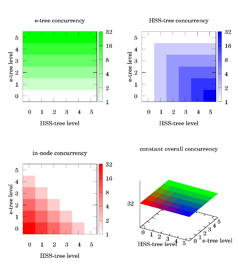This is illustrated in Figure 3. Even in the case of highly unbalanced trees, the runtime can assign work evenly to the available cores. We chose not to use an existing library for the task based dense linear algebra, for instance PLASMA (based on the QUARK runtime), since we wished to exploit the same threading mechanism (OpenMP) already used for the tree parallelism.

(a) Three nested levels of parallelism.

(b) Constant overall concurrency.

Figure 3: Schematic illustration of the different types of concurrency in the code and the gradual shift from tree parallelism to in-node parallelism. (a) Tasks for dense kernels ($\diamond$) are nested in nodes ($\circ$) of the HSS trees, which are nested in the elimination tree nodes ($\Box$) (e-tree). (b) Left-to-right, top-to-bottom: (1) Elimination tree concurrency decreases when getting closer to the root node. (2) Closer to the root of the elimination tree, more HSS tree concurrency is exploited as it becomes available, i.e., while moving down the HSS tree away from the root. (3) Towards the root of the HSS tree and the root of the elimination tree, more in-node concurrency (parallel tasked dense algebra) is exploited. (4) The product of the 3 types of concurrency, i.e., the overall concurrency, remains constant throughout both the elimination and HSS trees.

5.3 Parallel BLAS and LAPACK

One of the most time consuming operations of the algorithm is dense matrix-matrix multiplication $C\leftarrow\alpha AB+\beta C$. This can be implemented easily with recursion and task parallelism [41], by splitting the problem into smaller matrix-matrix multiplications; this strategy is referred to as divide-and-conquer and is often used in so-called cache-oblivious algorithms [26]. How the matrices are split depends on their shapes. Let $A$ be $m\times k$ and $B$ be $k\times n$, then

$$C\leftarrow\begin{cases}\alpha AB+\beta C&\textrm{if }m\times n\times k\leq T,\\ \alpha\begin{bmatrix}AB_{0}&AB_{1}\end{bmatrix}+\beta\begin{bmatrix}C_{0}&C_{1}\end{bmatrix}&\textrm{else if }n\geq\max(m,k),\\ \alpha\begin{bmatrix}A_{0}B\\ A_{1}B\end{bmatrix}+\beta\begin{bmatrix}C_{0}\\ C_{1}\end{bmatrix}&\textrm{else if }m\geq k,\\ \alpha\left(A_{0}B_{0}+A_{1}B_{1}\right)+\beta C&\textrm{else}\\ \end{cases}.$$ (20)

The last case in (20), short fat $A$ times tall skinny $B$, uses two consecutive recursive matrix-matrix multiplication calls. Cases 2 and 3 start two multiplications in parallel, spawning two tasks. The recursion ends when reaching case 1, with $T$ a tuning parameter set by default to $T=64^{3}$, where a sequential vendor optimized BLAS3 *gemm routine is called. Depending on the scalar type, one of four inlined template specialization functions for gemm<scalar> is executed to pick the correct version: sgemm, dgemm, cgemm or zgemm. For the other BLAS2/3 routines that are required, for instance triangular matrix multiplication and solve, a similar recursive approach is used. This recursive task generation is also stopped when the recursion depth becomes too large, with the same depth parameter being passed through the entire code and incremented each time it enters a new task.

The code also requires some LAPACK functionality, namely LQ, LU and RRQR decompositions. For those, we modify the reference Fortran LAPACK implementation to make use of our parallel (tasked) BLAS routines. Some vendor optimized LAPACK libraries do not just use the LAPACK reference code on top of multithreaded BLAS calls, but add additional optimizations to the LAPACK routines. Unfortunately, in our approach we cannot take advantage of these optimized multithreaded codes.

Figure 4: Speedups over sequential getrf from Intel^® MKL for matrices of size $500^{2}$ to $4000^{2}$. Left: Recursive LU decomposition using OpenMP tasked BLAS code. Middle: Reference LAPACK getrf using OpenMP tasked BLAS code. Right: MKL optimized multithreaded getrf. Our recursive implementation scales better than the reference netlib getrf with parallel BLAS but worse than the MKL optimized code. However, calling MKL multithreaded getrf from multiple threads simultaneously would lead to over-subscription and performance penalty. This is not a problem with the recursive LU because it uses the OpenMP task runtime, just like the rest of the code.

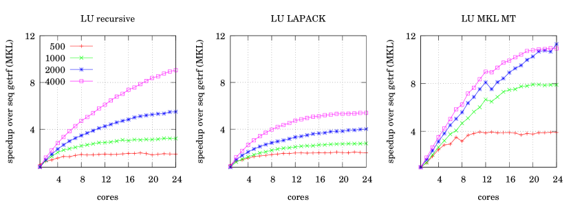
Consider partial pivoted LU decomposition, used for the $F_{11}$ block of a dense frontal matrix. Apart from the LAPACK *getrf routine using our OpenMP tasked BLAS routines, we also implemented a recursive LU factorization algorithm [21]. The parallelism in this algorithm has to come from the BLAS routines, triangular solve, row permutation, and matrix-matrix multiply. Figure 4 compares the performance and scalability of the two LU decomposition approaches with the MKL optimized implementation and shows our implementation of LU scales nearly as well as MKL without sacrificing the ability to exploit subtree concurrency. A more scalable approach [15], based on so-called tiled algorithms instead of recursion, partitions the matrices in tiles of fixed sizes and assigns tasks to each of the tiles while explicitly modeling the data dependencies between the tasks. A DAG (directed acyclic graph) scheduler then executes the tasks while respecting their dependencies. OpenMP supports explicit task dependencies since version 4.0. We intend to exploit this feature in the future to achieve more scalable dense linear algebra operations. For the rank-revealing QR decomposition we use a modified version of the LAPACK *geqp3 code [45], a BLAS3 version of column pivoted QR. The routine is modified to call our parallel tasked BLAS and an extra tolerance parameter $\varepsilon$ is added to stop the rank-revealing process as soon as the $\varepsilon$-rank has been found instead of computing the full decomposition. More precisely, numerical rank $i$ is detected when $R_{i+1,i+1}/R_{11}\leq\varepsilon$, where $R$ is the upper-triangular factor.

5.4 Scaling bottlenecks

Before the actual numerical factorization step, but after matrix scaling and nested dissection reordering, a symbolic factorization step is performed. During this step some memory is allocated and the index sets $I^{\mathrm{upd}}_{\tau}$ are assembled. The symbolic factorization is a bottom-up tree traversal which is done in parallel, as in Listing 1. In a multithreaded setting, memory allocation can become a serious scaling bottleneck. We have found that the use of a scalable memory allocator, like TCMalloc [27] or the TBB scalable memory allocator [46] greatly improves the performance over for instance the default malloc in glibc. For instance, running on a 60 core Intel^® Xeon Phi, the symbolic factorization phase runs up to $56\times$ faster when using TBBMalloc instead of the default allocator.

6 Numerical experiments

This section presents various numerical results. Section 6.1 first focuses on some PDE problems on regular grids as this allows us to easily change the problem size. The following sections consider other matrices from various applications. Unless otherwise stated, the experiments are performed on a single $12$-core socket of a single node of the NERSC Edison machine. A compute node has two $12$-core Intel^® Ivy Bridge processors at $2.4$GHz. Double precision peak performance is $19.2$Gflop/s per core, $230.4$Gflop/s per socket or $460.8$Gflop/s per node. Each socket has $32$GB DDR3 $1866$MHz memory, hence $64$GB per node, with a STREAM [40] bandwidth of $48.5$GB/s. We use the Intel^® 15.0.1 compiler with sequential MKL.

6.1 PDEs on a regular grid

We start with a number of benchmarks of well-known PDEs on regular 2D and 3D grids to study scaling of time-to-solution, number of floating point operations, memory usage, HSS-ranks etc., with respect to problem size. For these regular grids, a geometric nested dissection code is used instead of the default METIS graph partitioner. The following benchmark problems are considered:

• Poisson equation $-\Delta u=f$ on a 2D grid using the standard $5$-point finite difference stencil with homogeneous Dirichlet boundary conditions.

• Poisson equation on a 3D grid using the standard $7$-point stencil with homogeneous Dirichlet boundary conditions.

• Convection diffusion equation [43] $-\nu\Delta u+\mathbf{v}\cdot\nabla u=f$ on a 2D grid using a $5$-point upwind stencil, with viscosity $\nu=10^{-4}$ and

  $$\mathbf{v}=\begin{pmatrix}x(1-x)(2y-1)&y(1-y)(2x-1)\end{pmatrix}^{T}\,.$$ (21)

• Convection diffusion, similar as above, on 3D grid with

  $$\mathbf{v}=\begin{pmatrix}2x(1-x)(2y-1)z&-y(1-y)(2x-1)&-(2x-1)(2y-1)z(1-z)\end{pmatrix}^{T}\,.$$ (22)

• Helmholtz equation

  $$\left(-\Delta-\omega^{2}/v(x)^{2}\right)u(x,\omega)=s(x,\omega)$$ (23)

  on a 2D grid, with $\omega$ the angular frequency, $v(x)$ the seismic velocity and $u(x,\omega)$ the time-harmonic wavefield solution to the forcing term $s(x,\omega)$. The discretization uses a $9$-point stencil and the frequency is set at $f=10$Hz with $\omega=2\pi f$. We use a sampling rate of about $15$ points per wavelength and PML boundary conditions. This example uses complex arithmetic.

• Same as H2D, but 3D using a $27$-point stencil.

A crucial parameter for performance is the number of levels $\ell_{s}$ of the elimination tree for which HSS compression is performed. Note that $\ell_{s}=0$ corresponds to a pure multifrontal solver. Unfortunately, the optimal $\ell_{s}$ is impossible to predict a priori, so it is determined experimentally and will always be mentioned with each result. The same applies to the compression tolerance $\varepsilon$. When $\ell_{s}>0$, i.e., with HSS compression, the multifrontal solver is used as a preconditioner for restarted GMRES($30$) with modified Gram-Schmidt and a zero initial guess. Without HSS compression, iterative refinement with the direct solver is used. All experiments are performed in double precision with relative or absolute stopping criteria $\|u_{i}\|/\|u_{0}\|\leq 10^{-6}$ or $\|u_{i}\|\leq 10^{-10}$, where $u_{i}=M^{-1}(Ax_{i}-b)$, with $M$ the approximate multifrontal factorization of $A$, is the preconditioned residual. The right-hand-side is always set to $A\begin{bmatrix}1&1&\cdots&1\end{bmatrix}^{T}$.

(a) Num fact time, $5000^{2}$.

(b) Total solve time, $5000^{2}$.

(c) Num fact time, $125^{3}$.

(d) Total solve time, $125^{3}$.

Figure 5: Times for factorization (left) and solve (right) of the 2D (top) and 3D (bottom) Poisson equation on $5000^{2}$ and $125^{3}$ grids as function of the number of levels $\ell_{s}$ in the elimination tree for which HSS compression is applied. Different curves correspond to different HSS compression tolerances $\varepsilon$. For 3D, much more aggressive HSS compression can be used.

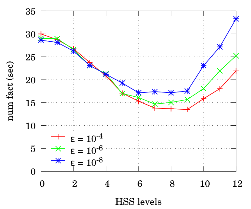
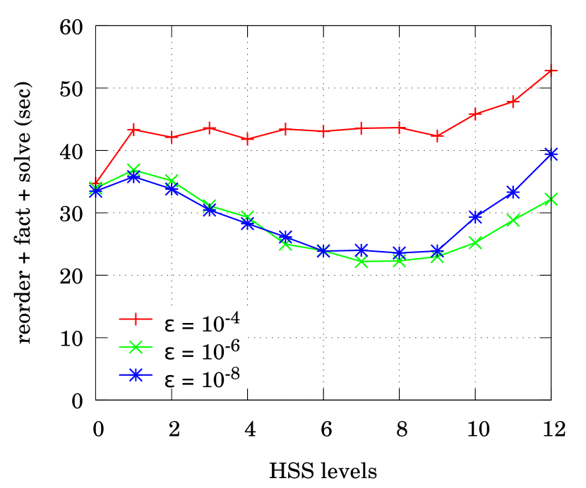
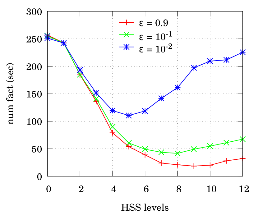
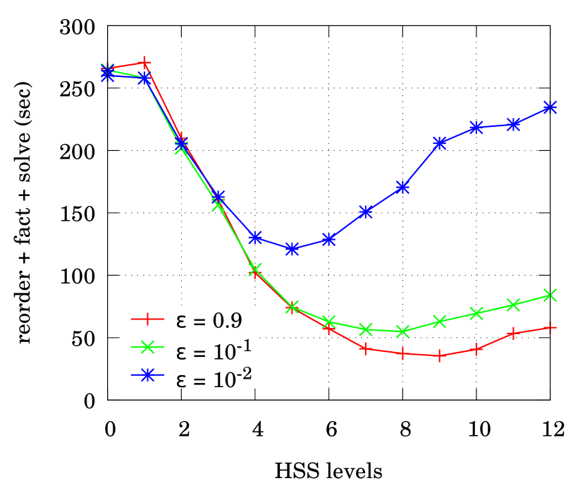
Figure 5 shows timing results for the 2D (top) and 3D (bottom) Poisson equation on $5000^{2}$ and $125^{3}$ grids respectively. Figure 5(a) shows numerical factorization time as a function of the number of levels in the elimination tree for which HSS compression was used. The HSS levels always correspond to the top levels of the elimination tree. This shows that applying HSS compression leads to a speedup of about $2\times$ for $7$ HSS levels. Different lines correspond to different HSS compression tolerances $\varepsilon$. Somewhat larger factorization speedups are possible for $\varepsilon\geq 10^{-4}$. However, this does not lead to faster time-to-solution. Figure 5(b) shows the cumulative time for nested dissection reordering, symbolic factorization, numerical factorization and GMRES solve. For $\varepsilon\geq 10^{-4}$, the number of GMRES iterations, and thus the number of applications of the multifrontal solve, increases too much to get overall speedup. Best results were obtained with $\ell_{s}=8$, $\varepsilon=10^{-7}$ and only $2$ GMRES iterations ($3$ multifrontal solves). Figures 5(c) and 5(d) show the timings for the 3D Poisson problem. For the 3D problem, much more aggressive HSS compression can be used. Best results were obtained with $\ell_{s}=10$, $\varepsilon=0.9$ and $61$ GMRES iterations. For the Poisson problem it seems that for 2D the direct solver is very efficient, with a modest speedup from HSS, while for 3D the HSS enabled factorization leads to a good preconditioner.

(a) 2D Poisson.

(b) 3D Poisson.

Figure 6: Scaling of the number of floating point operations required to factor and solve a 2D(a) or 3D(b) Poisson equation. (a) The theory predicts $\mathcal{O}(N^{3/2})$ complexity for the multifrontal (MF) solver and optimal $\mathcal{O}(N)$ [55] complexity with HSS compression. (b) $\mathcal{O}(N^{2})$ complexity for the multifrontal solver and slightly lower complexity with HSS compression. The fits (black lines) are very sensitive to the data and not very reliable. However, note the smaller exponents and the larger constants for the new solver.

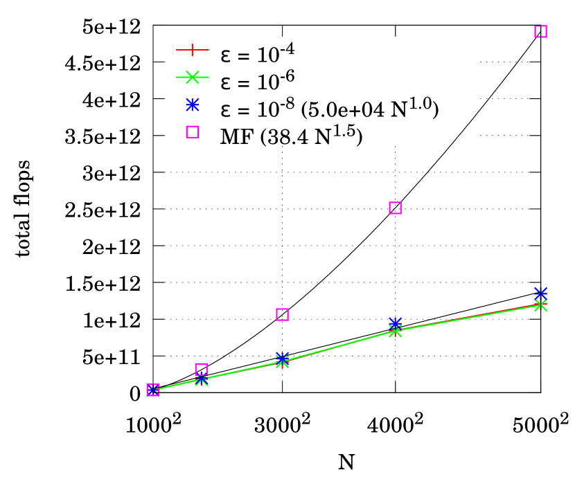
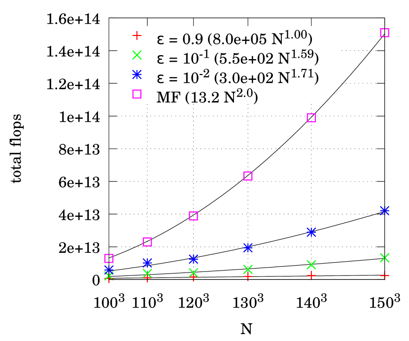
Figure 6(a) shows the total number of flops (numerical factorization and GMRES solve) for solving a 2D Poisson equation as function of the number of degrees of freedom, again for different compression tolerances. For the pure multifrontal method (no compression), the number of flops is $\mathcal{O}(N^{3/2})$, as predicted by the theory. For 2D Poisson the HSS-rank is independent of the grid size [17], which leads to an optimal solver, i.e., linear scaling in the number of unknowns, see the fit in Figure 6(a). Note the much larger constant for the HSS method. For the $5000^{2}$ problem there is a reduction in the number of flops by a factor of about $3.3\times$. However, the observed speedup (Figure 5(b)) is smaller than that. This is due to the fact that although the number of flops for the factorization decreases, the number of flops for the solution phase (and GMRES iterations) increases. Although multifrontal solve requires an order of magnitude less flops than factorization, it runs at much lower flop rates on modern hardware because it is limited by the memory bandwidth instead of the floating point unit. Additionally, the flop rate in the factorization phase is lower when using HSS compression due to the more fine-grained task decomposition. Figure 6(b) shows number of flops-to-solution for the 3D Poisson equation. For the very aggressive compression, $\varepsilon=0.9$, the number of floating point operations for the $125^{3}$ problem are reduced to $4.4\%$ of the number of flops for the multifrontal method.

(a) 3D Poisson, total time.

(b) 3D Poisson, factor size.

Figure 7: (a) Total solve time (reordering, factorization and solution) for the 3D $125^{3}$ Poisson equation. (b) Factor size for the same problem. Different lines correspond to different HSS compression tolerance $\varepsilon$, MF refers to pure multifrontal. The HSS enabled solver is faster for larger problems, and it allows to solve larger problems.

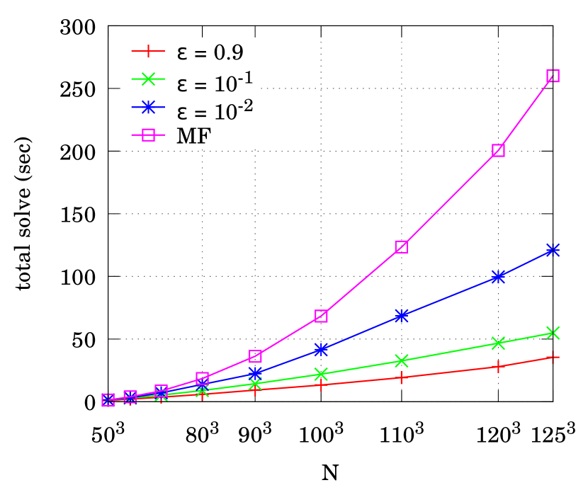
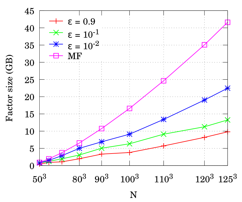
Figure 7(a) shows the total solve time for the 3D problem for different grid sizes. These times include matrix reordering, factorization and GMRES solve. Figure 7(b) shows the size of the factors.

problem		P2D	P3D	C2D	C3D	H2D	H3D
grid size		$5000^{2}$	$125^{3}$	$5000^{2}$	$125^{3}$	$4000^{2}$	$100^{3}$
Multifrontal	nested dissection time (s)	2.5	0.25	2.1	0.24	2.9	0.43
	symbolic factorization time (s)	3.6	8.0	3.4	8.1	4.5	6.0
	factorization time (s)	29.1	254.7	28.8	252.4	53.6	259.1
	factorization flops ($\times 10^{12}$)	4.9	50.0	4.9	50.0	10.1	53.5
	flop rate ($\times 10^{9}$Gflop/s)	168.4	196.3	170.1	198.1	188.4	206.5
	fraction of peak	73%	85%	74%	86%	82%	90%
	factor size (GB)	28.4	41.6	28.4	41.6	36.3	35.5
	solution time (s)	1.4	1.1	1.5	1.1	2.4	0.91
	solution flops ($\times 10^{9}$)	7.9	10.5	7.9	10.5	21.1	18.2
	solution bandwidth (GB/s)	20.3	37.8	18.9	37.8	15.1	39.0
	fraction of peak	42%	78%	39%	78%	31%	80%
	total flops ($\times 10^{12}$)	4.9	50.0	4.9	50.0	10.1	53.5
	total time (s)	36.6	264.1	35.8	261.8	63.4	266.4
Multifrontal + HSS	nested dissection time (s)	2.5	0.26	2.1	0.24	2.9	0.43
	separator reordering time (s)	1.1	0.40	1.1	0.35	1.3	0.68
	symbolic factorization time (s)	2.0	0.55	2.1	0.8	2.9	1.8
	factorization time (s)	14.5	19.6	13.6	41.5	30.5	92.8
	factorization flops ($\times 10^{12}$)	1.5	2.0	1.3	5.0	3.9	18.0
	flop rate ($\times 10^{9}$Gflop/s)	103.4	102.0	95.6	120.5	127.9	194.0
	fraction of peak	45%	44%	41%	52%	56%	84%
	factor size (GB)	22.5	9.8	21.6	14.6	29.6	21.4
	fraction of multifrontal	79%	24%	76%	35%	82%	60%
	solution time (s)	4.1	15.3	4.3	75.9	22.5	71.2
	GMRES(30) iterations	3	67	3	234	11	152
	solution flops ($\times 10^{9}$)	25.6	169.9	23.7	876.3	210.5	1,759.0
	solution bandwidth (GB/s)	22.0	43.6	20.1	45.2	15.8	46.0
	fraction of peak	45%	90%	41%	93%	33%	95%
	HSS levels $\ell_{s}$ (total)	7 (22)	8 (18)	8 (22)	7 (18)	7 (22)	4 (18)
	HSS-rank	48	46	50	397	139	30
	HSS compression tolerance $\varepsilon$	$10^{-6}$	0.9	$10^{-5}$	0.1	$10^{-4}$	0.9
	total flops ($\times 10^{12}$)	1.5	2.2	1.3	5.9	4.1	19.8
	fraction of multifrontal	30%	4.4%	27%	12%	41%	37%
	total time (s)	24.2	36.1	23.2	118.8	60.1	166.9
	speedup	1.52$\times$	7.14$\times$	1.54$\times$	2.22$\times$	1.05$\times$	1.59$\times$

Table 2: Comparison of the standard multifrontal solver and the multifrontal solver with HSS compression for a number of PDEs on regular grids. All experiments are run on a $12$-core Intel^® Ivy Bridge (peak $230.4$Gflop/s and $48.5$GB/s) in double precision. The code achieves good performance in terms of Gflop/s (for the factorization) or GByte/s (for the solve) and HSS compression leads to nice speedups over the standard multifrontal solver. A geometric nested dissection code is used for these regular grid problems.

Table 2 shows detailed results for the 6 PDE problems. The best speedups are obtained for the 3D problems. The code achieves good performance in flops per second for the factorization phase; although slightly less so for the HSS enabled code. Since the performance of the solve phase is not bounded by the floating point unit but rather by the memory bandwidth, we report the approximate attained bandwidth. The detailed results from Table 2 are summarized in Figure 8.

Figure 8: Summary of the results from Table 2: Poisson (P), convection-diffusion (C) and Helmholtz (H) on 2D (left) and 3D (right) regular grids on a $12$-core Intel^® Ivy Bridge. Poisson and convection-diffusion are in double precision, Helmholtz in complex double precision.

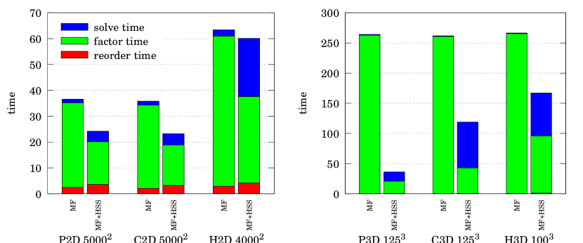
The $\varepsilon$ and $\ell_{s}$ values used for Table 2 and Figures 5-7 were chosen to minimize the total time to factor and solve a single linear system, i.e., the optimal trade-off between factorization time and number of GMRES iterations. When multiple consecutive solves with the same matrix are required, one needs to select different $\ell_{s}$ and $\varepsilon$ values. For many consecutive and highly accurate solves, the pure (exact) multifrontal factorization is probably optimal as it minimizes the number of multifrontal triangular solves. However, suppose only a few digits of accuracy are required. The multifrontal HSS solver can be used as a direct solver and due to the smaller factor size the solve phase will be faster than a solve with the pure multifrontal code.

The times for symbolic factorization in Table 2 are larger for the multifrontal method than for the HSS solver. This is because the memory for dense frontal matrices is allocated during the symbolic factorization while memory for the HSS generators is allocated during the numerical factorization since HSS-ranks are not known in advance.

6.2 Matrices from various applications

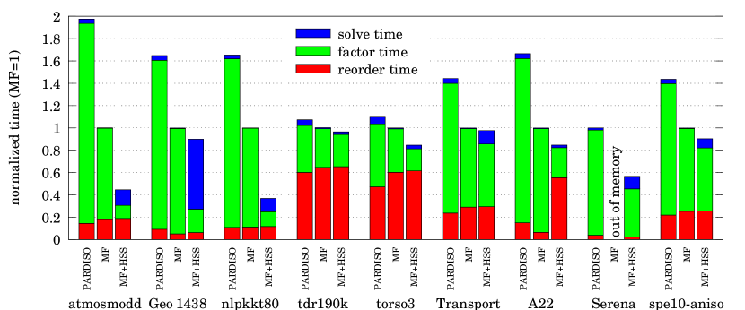
Figure 9 shows a comparison of timings to solve linear systems with a number of matrices from applications. The matrices atmosmodd, Geo_1438, nlpkkt80, torso3, Transport and Serena are from the University of Florida Sparse Matrix Collection. The other matrices tdr190k, A22 and spe10-anisotropic, are from SciDAC projects at the DOE. The matrices are also listed in Table 3, which additionally contains matrix Cube_Coup_dt0. This last matrix is not shown in Figure 9 because our multifrontal code ran out of memory during factorization unless HSS compression was used. All selected matrices are relatively large and originated from a 2D or 3D partial differential equation (on arbitrary domains). In Figure 9, our HSS enabled multifrontal solver (MF+HSS) is compared to the pure multifrontal method (MF) and to the state-of-the-art PARDISO solver [49]. PARDISO, a multithreaded supernodal solver, is part of Intel^® MKL. For MF and MF+HSS, reorder time includes nested dissection, MC64 and symmetrization of the sparsity structure and for MF+HSS also separator reordering. Factor time includes both symbolic and numerical factorization. The times are normalized to a total time $1$ for MF. For the matrices selected for Figure 9, we see a consistent speedup from MF+HSS compared to pure MF and our MF solver always outperforms the PARDISO solver. PARDISO uses the same METIS nested dissection reordering as our implementation, with comparable reordering times for the different solvers. The supernodal pivoting scheme used in PARDISO for numerical stability does not affect the fill-in so the overall number of nonzeros in the factors with PARDISO and with our multifrontal code are very similar. Only for the A22 problem reordering the separator in order to reduce the HSS-ranks takes a lot of time. This is probably due to the addition of link-two edges to the separator graph (see Section 4.2) since the original matrix already has 246 nonzeros per row on average. However, if those extra edges are not taken into account, the HSS-ranks are much larger and there is no net performance benefit from using HSS.

Figure 9: Comparison of timings for matrices from various applications on a $12$-core Intel^® Ivy Bridge. PARDISO is the sparse direct multithreaded solver from Intel^® MKL. MF refers to our implementation of the multifrontal method and MF+HSS is our new multifrontal solver with HSS compression. The matrices are taken from the Florida Sparse Matrix Collection and from SciDAC projects at the DOE. For these matrices, which are all quite large and from 2D/3D PDE problems, our MF solver is faster than PARDISO and HSS compression gives an additional speedup.

			MF		HSS
matrix	order	#nnz	factor	solve	$\ell_{s}/\ell_{\textrm{max}}$	$\varepsilon$	rank	its	factor	solve
atmosmodd	1.2M	8.8M	81s	0.4s	6/18	$0.9$	17	88	25s	11s
Geo_1438	1.4M	63M	205s	1s	6/18	$0.9$	8	318	56s	129s
nlpkkt80	1.1M	29M	197s	0.7s	6/18	$0.5$	59	90	49s	23s
tdr190k	1.1M	43M	19s	0.2s	1/18	$10^{-4}$	61	2	18s	0.4s
torso3	.25M	4.4M	6s	0.05s	6/15	$0.5$	36	7	5s	0.2s
Transport	1.6M	23M	80s	0.5s	3/18	$10^{-2}$	182	24	69s	10s
A22	.59M	145M	127s	0.7s	10/17	$0.1$	172	18	105s	3s
spe10-aniso	1.2M	31M	88s	0.4s	3/18	$10^{-2}$	245	21	73s	7.3s
Serena*	1.4M	65M	171s	0.5s	6/18	$0.9$	11	111	40s	22s
Cube_Coup_dt0*	2.2M	65M	-	-	8/19	$0.5$	100	200	60s	63s
*single precision experiment

Table 3: Same as in Figure 9: comparison of timings for matrices from various applications on a $12$-core Intel^® Ivy Bridge. This table also shows the optimal number of HSS levels $\ell_{s}$, the optimal compression tolerance $\varepsilon$ and the corresponding HSS-rank and number of GMRES($30$) iterations. For the Serena and Cube_Coup_dt0 matrices the pure multifrontal method ran out of memory in double precision.

6.3 Many-core parallel performance

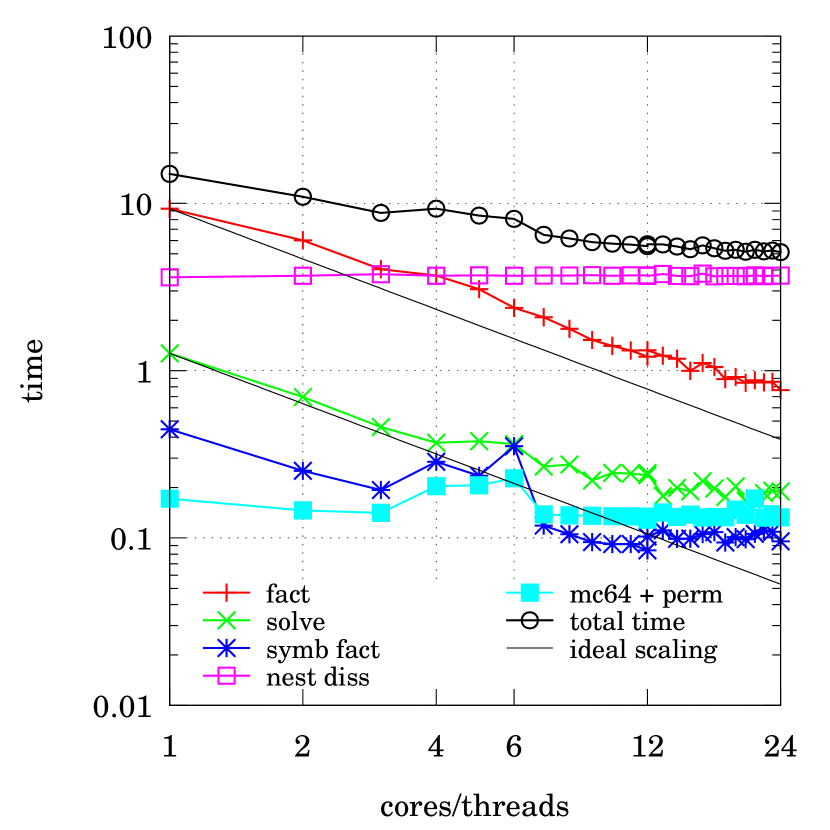
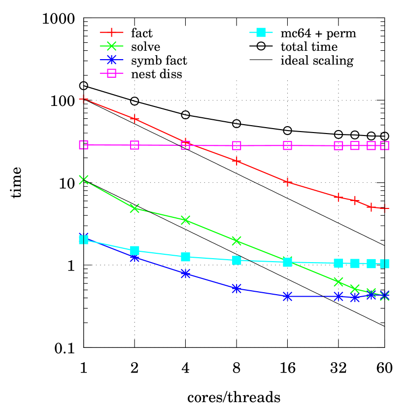
Figure 10 shows performance and parallel scalability of the MF+HSS solver applied to the torso3.mtx matrix ($\ell_{s}=6$, $\varepsilon=0.5$) on two leading multi-core architectures: a two sockets machine with a $12$-core Intel^® Ivy Bridge Xeon per socket and a $60$-core Intel^® Xeon Phi Knight’s Corner. When running $12$ or less threads on the dual socket $24$-core Xeon system, the threads are all bound to a single socket (NUMA node). Note that since the Xeon Phi only has $8$GB of memory, the larger problems from Table 3 do not fit in it’s memory. Our code shows good parallel scalability on both architectures for the numerical factorization phase and reasonable scalability for the solve phase. However, with increasing number of threads the reordering codes MC64 and METIS/SCOTCH quickly become scaling bottlenecks. The MC64 phase in Figure 10 shows some parallel speedup since this time also includes applying the column permutation from MC64, which is done in parallel.

(a) Intel^® Ivy Bridge.

(b) Intel^® Xeon Phi.

Figure 10: Multi-core scalability of the different steps in the MF+HSS solver on two leading architectures. The MF+HSS solver is applied to the relatively small torso3.mtx matrix. The code achieves good speedup for the numerical factorization phase and reasonable speedup for the solve (MF+HSS preconditioned GMRES). Note that the sequential reordering codes METIS and MC64 become bottlenecks.

7 Conclusions & Outlook

We presented an initial attempt to create a high performance implementation of a novel multifrontal solver with HSS low-rank structures. We show speedups of up to $7\times$ over the pure multifrontal algorithm for a range of applications. Moreover, our implementation compares favorably to the commercial PARDISO solver. We observed that the new solver has lower computational complexity than the pure multifrontal method. However, the constants involved are much larger. We will focus our attention on trying to reduce these constants (for instance by trying to reduce the HSS-ranks) and on solving larger problems with a distributed memory implementation. As possible strategies to reduce the HSS-ranks we consider the following. A power iteration on the random vectors, for instance $S^{r}=\left(AA^{*}\right)^{q}AR$ with $q$ a small integer, will improve the quality of the samples at the expense of additional computations; see [29] for further details. We believe the separator reordering, see Section 4.2, can be improved, perhaps by taking into account the matrix entries and/or the underlying geometry, also leading to lower ranks. Finally, a better rank-revealing factorization, like a strong rank-revealing QR [28], might lead to lower ranks and possibly more stable ULV factorization. The solver with HSS compression achieves lower floating point operation throughput than the pure multifrontal code. Hence, we believe there is some room for improvement. We will continue performance tuning of the code on various modern computer architectures.

The presented code is part of a package called STRUMPACK. At the moment STRUMPACK has a sparse shared memory solver and a dense distributed memory solver. The longer term goal is to develop and maintain a single scalable code for both sparse and dense problems using hybrid parallelism. The current paper, together with the distributed HSS code developed for [47] are a good step towards reaching that goal.

The research on fast sparse and dense direct solvers is a very active field at the moment. Some newer algorithmic ideas are for instance nested HSS approximation and matrix-free direct solver-based preconditioners. In nested HSS approximation, the HSS generators of the frontal matrices are themselves HSS matrices. This could further reduce the overall complexity of the solver. A matrix-free direct solver based preconditioner could be constructed using randomization techniques. It seems that knowledge of the sparsity pattern would be required for this.

References

- [1] Emmanuel Agullo, Alfredo Buttari, Abdou Guermouche, and Florent Lopez. Multifrontal QR factorization for multicore architectures over runtime systems. In Euro-Par 2013 Parallel Processing, pages 521–532. Springer, 2013.
- [2] Emmanuel Agullo, Jim Demmel, Jack Dongarra, Bilel Hadri, Jakub Kurzak, Julien Langou, Hatem Ltaief, Piotr Luszczek, and Stanimire Tomov. Numerical linear algebra on emerging architectures: The plasma and magma projects. In Journal of Physics: Conference Series, volume 180, page 012037. IOP Publishing, 2009.
- [3] Sivaram Ambikasaran. Fast Algorithms for Dense Numerical Linear Algebra and Applications. PhD thesis, Stanford, 2013.
- [4] Patrick R Amestoy, Cleve Ashcraft, Olivier Boiteau, Alfredo Buttari, Jean-Yves L’Excellent, and Clément Weisbecker. Improving multifrontal methods by means of block low-rank representations. To appear in SIAM Journal on Scientific Computing, 2015.
- [5] Patrick R Amestoy, Tim A Davis, and Iain S Duff. An approximate minimum degree ordering algorithm. SIAM Journal on Matrix Analysis and Applications, 17(4):886–905, 1996.
- [6] Patrick R Amestoy, Iain S Duff, Jean-Yves L’Excellent, and Jacko Koster. A fully asynchronous multifrontal solver using distributed dynamic scheduling. SIAM Journal on Matrix Analysis and Applications, 23(1):15–41, 2001.
- [7] Patrick R Amestoy, Iain S Duff, Daniel Ruiz, and Bora Uçar. A parallel matrix scaling algorithm. In High Performance Computing for Computational Science-VECPAR 2008, pages 301–313. Springer, 2008.
- [8] Amirhossein Aminfar, Sivaram Ambikasaran, and Eric Darve. A fast block low-rank dense solver with applications to finite-element matrices. CoRR, abs/1403.5337, 2014.
- [9] Cédric Augonnet, Samuel Thibault, Raymond Namyst, and Pierre-André Wacrenier. StarPU: a unified platform for task scheduling on heterogeneous multicore architectures. Concurrency and Computation: Practice and Experience, 23(2):187–198, 2011.
- [10] Mario Bebendorf. Approximation of boundary element matrices. Numerische Mathematik, 86(4):565–589, 2000.
- [11] Robert D Blumofe, Christopher F Joerg, Bradley C Kuszmaul, Charles E Leiserson, Keith H Randall, and Yuli Zhou. Cilk: An efficient multithreaded runtime system. Journal of parallel and distributed computing, 37(1):55–69, 1996.
- [12] Robert D Blumofe and Charles E Leiserson. Scheduling multithreaded computations by work stealing. Journal of the ACM (JACM), 46(5):720–748, 1999.
- [13] Steffen Börm, Lars Grasedyck, and Wolfgang Hackbusch. Introduction to hierarchical matrices with applications. Engineering Analysis with Boundary Elements, 27(5):405–422, 2003.
- [14] George Bosilca, Aurelien Bouteiller, Anthony Danalis, Thomas Herault, Pierre Lemarinier, and Jack Dongarra. Dague: A generic distributed dag engine for high performance computing. Parallel Computing, 38(1):37–51, 2012.
- [15] Alfredo Buttari, Julien Langou, Jakub Kurzak, and Jack Dongarra. A class of parallel tiled linear algebra algorithms for multicore architectures. Parallel Computing, 35(1):38–53, 2009.
- [16] Tony F Chan. Rank revealing QR factorizations. Linear Algebra and Its Applications, 88:67–82, 1987.
- [17] Shivkumar Chandrasekaran, Patrick Dewilde, Ming Gu, and N Somasunderam. On the numerical rank of the off-diagonal blocks of Schur complements of discretized elliptic PDEs. SIAM Journal on Matrix Analysis and Applications, 31(5):2261–2290, 2010.
- [18] Shivkumar Chandrasekaran, Ming Gu, and Timothy Pals. A fast ULV decomposition solver for hierarchically semiseparable representations. SIAM Journal on Matrix Analysis and Applications, 28(3):603–622, 2006.
- [19] Hongwei Cheng, Zydrunas Gimbutas, Per-Gunnar Martinsson, and Vladimir Rokhlin. On the compression of low rank matrices. SIAM Journal on Scientific Computing, 26(4):1389–1404, 2005.
- [20] A R Curtis and John Ker Reid. On the automatic scaling of matrices for Gaussian elimination. IMA Journal of Applied Mathematics, 10(1):118–124, 1972.
- [21] Jack Dongarra, Mathieu Faverge, Hatem Ltaief, and Piotr Luszczek. Achieving numerical accuracy and high performance using recursive tile lu factorization with partial pivoting. Concurrency and Computation: Practice and Experience, 26(7):1408–1431, 2014.
- [22] Iain S Duff and Jacko Koster. The design and use of algorithms for permuting large entries to the diagonal of sparse matrices. SIAM Journal on Matrix Analysis and Applications, 20(4):889–901, 1999.
- [23] Iain S Duff and John Ker Reid. The multifrontal solution of indefinite sparse symmetric linear. ACM Transactions on Mathematical Software (TOMS), 9(3):302–325, 1983.
- [24] Alejandro Duran, Eduard Ayguadé, Rosa M Badia, Jesús Labarta, Luis Martinell, Xavier Martorell, and Judit Planas. Ompss: a proposal for programming heterogeneous multi-core architectures. Parallel Processing Letters, 21(02):173–193, 2011.
- [25] B. Engquist and L. Ying. Sweeping preconditioner for the helmholtz equation: hierarchical matrix representation. Commun. Pure Appl. Math., 64:697–735, 2011.
- [26] Matteo Frigo, Charles E Leiserson, Harald Prokop, and Sridhar Ramachandran. Cache-oblivious algorithms. In Foundations of Computer Science, 1999. 40th Annual Symposium on, pages 285–297. IEEE, 1999.
- [27] Sanjay Ghemawat and Paul Menage. Tcmalloc: Thread-caching malloc. goog-perftools. sourceforge. net/doc/tcmalloc. html, 2009.
- [28] Ming Gu and Stanley C Eisenstat. Efficient algorithms for computing a strong rank-revealing QR factorization. SIAM Journal on Scientific Computing, 17(4):848–869, 1996.
- [29] Nathan Halko, Per-Gunnar Martinsson, and Joel A Tropp. Finding structure with randomness: Probabilistic algorithms for constructing approximate matrix decompositions. SIAM review, 53(2):217–288, 2011.
- [30] Pascal Hénon, Pierre Ramet, and Jean Roman. PaStiX: a high-performance parallel direct solver for sparse symmetric positive definite systems. Parallel Computing, 28(2):301–321, 2002.
- [31] Jonathan D Hogg, John K Reid, and Jennifer A Scott. Design of a multicore sparse Cholesky factorization using DAGs. SIAM Journal on Scientific Computing, 32(6):3627–3649, 2010.
- [32] George Karypis and Vipin Kumar. A fast and high quality multilevel scheme for partitioning irregular graphs. SIAM Journal on scientific Computing, 20(1):359–392, 1998.
- [33] Kyungjoo Kim and Victor Eijkhout. A parallel sparse direct solver via hierarchical DAG scheduling. ACM Transactions on Mathematical Software (TOMS), 41(1):3, 2014.
- [34] Ronald Kriemann. -LU factorization on many-core systems. Computing and Visualization in Science, 16(3):105–117, 2013.
- [35] Xavier Lacoste, Mathieu Faverge, George Bosilca, Pierre Ramet, and Samuel Thibault. Taking advantage of hybrid systems for sparse direct solvers via task-based runtimes. In Parallel & Distributed Processing Symposium Workshops (IPDPSW), 2014 IEEE International, pages 29–38. IEEE, 2014.
- [36] Jean-Yves L’Excellent. Multifrontal Methods: Parallelism, Memory Usage and Numerical Aspects. Habilitation à diriger des recherches, École normale supérieure de Lyon, September 2012.
- [37] Lin Lin, Jianfeng Lu, and Lexing Ying. Fast construction of hierarchical matrix representation from matrix–vector multiplication. Journal of Computational Physics, 230(10):4071–4087, 2011.
- [38] Joseph W. H. Liu. The multifrontal method for sparse matrix solution: Theory and practice. SIAM review, 34(1):82–109, 1992.
- [39] Per-Gunnar Martinsson. A fast randomized algorithm for computing a hierarchically semiseparable representation of a matrix. SIAM Journal on Matrix Analysis and Applications, 32(4):1251–1274, 2011.
- [40] John D McCalpin. STREAM: Sustainable Memory Bandwidth in High Performance Computers. http://www.cs.virginia.edu/stream/.
- [41] Michael McCool, James Reinders, and Arch Robison. Structured parallel programming: patterns for efficient computation. Elsevier, 2012.
- [42] Artem Napov and Xiaoye S Li. An algebraic multifrontal preconditioner that exploits the low-rank property. Submitted to Numerical Linear Algebra with Applications, 2013.
- [43] Y. Notay. An aggregation-based algebraic multigrid method. Electronic Trans. Numer. Anal., 37:123–146, 2010.
- [44] François Pellegrini and Jean Roman. Scotch: A software package for static mapping by dual recursive bipartitioning of process and architecture graphs. In High-Performance Computing and Networking, pages 493–498. Springer, 1996.
- [45] Gregorio Quintana-Ortí, Xiaobai Sun, and Christian H Bischof. A BLAS-3 version of the QR factorization with column pivoting. SIAM Journal on Scientific Computing, 19(5):1486–1494, 1998.
- [46] James Reinders. Intel threading building blocks: outfitting C++ for multi-core processor parallelism. O’Reilly Media, Inc., 2007.
- [47] François-Henry Rouet, Xiaoye S. Li, Pieter Ghysels, and Artem Napov. A distributed-memory package for dense Hierarchically Semi-Separable matrix computations using randomization. submitted to ACM Transactions on Mathematical Software, 2014.
- [48] Daniel Ruiz. A scaling algorithm to equilibrate both rows and columns norms in matrices. Technical report, Technical Report RT/APO/01/4, ENSEEIHT-IRIT, 2001. Also appeared as RAL report RAL-TR-2001-034, 2001.
- [49] Olaf Schenk, Klaus Gärtner, and Wolfgang Fichtner. Efficient sparse lu factorization with left-right looking strategy on shared memory multiprocessors. BIT Numerical Mathematics, 40(1):158–176, 2000.
- [50] Raf Vandebril, Marc Van Barel, Gene Golub, and Nicola Mastronardi. A bibliography on semiseparable matrices. Calcolo, 42(3-4):249–270, 2005.
- [51] Shen Wang, Maarten V de Hoop, and Jianlin Xia. On 3D modeling of seismic wave propagation via a structured parallel multifrontal direct Helmholtz solver. Geophysical Prospecting, 59(5):857–873, 2011.
- [52] Shen Wang, Xiaoye S Li, François-Henry Rouet, Jianlin Xia, and Maarten V De Hoop. A parallel geometric multifrontal solver using hierarchically semiseparable structure. submitted to ACM Transactions on Mathematical Software, 2014.
- [53] Clément Weisbecker. Improving multifrontal solvers by means of algebraic Block Low-Rank representations. PhD thesis, Institut National Polytechnique de Toulouse, 2013.
- [54] James Hardy Wilkinson. Rounding errors in algebraic processes. Courier Dover Publications, 1994.
- [55] Jianlin Xia. Randomized sparse direct solvers. SIAM Journal on Matrix Analysis and Applications, 34(1):197–227, 2013.
- [56] Jianlin Xia, Shivkumar Chandrasekaran, Ming Gu, and Xiaoye S Li. Fast algorithms for hierarchically semiseparable matrices. Numerical Linear Algebra with Applications, 17(6):953–976, 2010.
- [57] Jianlin Xia, Yuanzhe Xi, and Ming Gu. A superfast structured solver for Toeplitz linear systems via randomized sampling. SIAM Journal on Matrix Analysis and Applications, 33(3):837–858, 2012.
- [58] Asim YarKhan, Jakub Kurzak, and Jack Dongarra. Quark users’ guide: Queueing and runtime for kernels. University of Tennessee Innovative Computing Laboratory Technical Report ICL-UT-11-02, 2011.