Abstract

A classic tension exists between exact inference in a simple model and approximate inference in a complex model. The latter offers expressivity and thus accuracy, but the former provides coverage of the space, an important property for confidence estimation and learning with indirect supervision. In this work, we introduce a new approach, reified context models, to reconcile this tension. Specifically, we let the amount of context (the arity of the factors in a graphical model) be chosen “at run-time” by reifying it—that is, letting this choice itself be a random variable inside the model. Empirically, we show that our approach obtains expressivity and coverage on three natural language tasks.

1 Introduction

Many structured prediction tasks across natural language processing, computer vision, and computational biology can be formulated as that of learning a distribution over outputs $y_{1:L}=(y_{1},\dots,y_{L})\in\mathcal{Y}_{1:L}$ given an input $x$:

$$p_{\theta}(y_{1:L}\mid x)\propto\exp\left(\sum_{i=1}^{L}\theta^{\top}\phi_{i}(y_{1:i-1},y_{i},x)\right).$$ (1)

The thirst for expressive models (e.g., where $y_{i}$ depends heavily on its context $y_{1:i-1}$) often leads one down the route of approximate inference, for example, to Markov chain Monte Carlo Brooks et al. (2011), sequential Monte Carlo Cappé et al. (2007); Doucet & Johansen (2011), or beam search Koehn et al. (2003). While these methods in principle can operate on models with arbitrary amounts of context, they only touch a small portion of the output space $\mathcal{Y}_{1:L}$. Without such coverage, we miss out on two important but oft-neglected properties:

• precision: In user-facing applications, it is important to only predict on inputs where the system is confident, leaving hard decisions to the user (Zhang et al., 2014). Lack of coverage means failing to consider all alternative outputs, which leads to overconfidence and poor estimates of uncertainty.

• indirect supervision: When only part of the output $y_{1:L}$ is observed, lack of coverage is even more problematic than it is in the fully-supervised setting. An approximate inference algorithm might not even consider the true $y$ (whereas one always has the true $y$ in a fully-supervised setting), which leads to invalid parameter updates (Yu et al., 2013).

Of course, lower-order models admit exact inference and ensure coverage, but these models have unacceptably low expressive power. Ideally, we would like a model that varies the amount of context in a judicious way, allocating modeling power to parts of the input that demand it. Therein lies the principal challenge: How can we adaptively choose the amount of context for each position $i$ in a data-dependent way while maintaining tractability?

In this paper, we introduce a new approach, which we call reified context models. The key idea is based on reification, a general idea in logic and programming languages, which refers to making something previously unaccessible (e.g., functions or metadata of functions) a “first-class citizen” and therefore available (e.g., via lambda abstraction or reflection) to formal manipulation. In the probabilistic modeling setting, we propose reifying the contexts as random variables in the model so that we can reason over them.

r	ro	rol	*olc	$\bullet\ \bullet\ \bullet\ \bullet\ \bullet\ \bullet\ \bullet\ \bullet\ \bullet$
v	ra	ral	***c
y	*o	*ol	***r
*	**	***	****

Figure 1: Illustration of our method for handwriting recognition. At each position, we keep track of a collection of contexts, and learn a model that factorizes with respect to these contexts. Each context remembers a certain amount of history, e.g. $\star o$ is all length two sequences whose second character is $o$. By using contexts at multiple levels of resolution, we can obtain coverage of the entire space while still modeling complex dependencies.

Specifically, for each $i\in\{1,\ldots,L-1\}$, we maintain a collection $\mathcal{C}_{i}$ of contexts, each of which is a subset of $\mathcal{Y}_{1:i}$ representing what we remember about the past (see Figure 1 for an example). We define a joint model over $(y,c)$, suppressing $x$ for brevity:

$$p_{\theta}(y_{1:L},c_{1:L-1})\propto\exp\left(\sum_{i=1}^{L}\theta^{\top}\phi_{i}(c_{i-1},y_{i})\right)\times\kappa(y,c),$$ (2)

where $\kappa$ is a consistency potential, to be explained later. The features $\phi_{i}$ now depend on the current context $c_{i-1}$, rather than the full history $y_{1:i-1}$. The distribution over $(y,c)$ factorizes according to the graphical model below:

(3)

The factorization (3) implies that the family in (2) admits efficient exact inference via the forward-backward algorithm as long as each collection $\mathcal{C}_{i}$ has small cardinality.

Adaptive selection of context.

Given limited computational resources, we only want to track contexts that are reasonably likely to contain the answer. We do this by selecting the context sets $\mathcal{C}_{i}$ during a forward pass using a heuristic similar to beam search, but unlike beam search, we achieve coverage because we are selecting contexts rather than individual variable values. We detail our selection method, called RCMS, in Section 4. We can think of selecting the $\mathcal{C}_{i}$’s as selecting a model to perform inference in, with the guarantee that all such models will be tractable. Our method is simple to implement; see the appendix for implementation details.

The goal of this paper is to flesh out the framework described above, providing intuitions about its use and exploring its properties empirically. To this end, we start in Section 2 by defining some tasks that motivate this work. In Sections 3 and 4 we introduce reified context models formally, together with an algorithm, RCMS, for selecting contexts adaptively at run-time. Sections 5-7 explore the empirical properties of the RCMS method. Finally, we discuss future research directions in Section 9.

2 Description of Tasks

To better understand the motivation for our work, we present three tasks of interest, which are also the tasks used in our empirical evaluation later. These tasks are word recognition (a fully supervised task), speech recognition (a weakly supervised task), and decipherment (an unsupervised task). The first of these tasks is relatively easy while the latter two are harder. We use word recognition to study the precision of our method, the other two tasks to explore learning under indirect supervision, and all three to understand how our algorithm selects contexts during training.

Word recognition

The first task is the word recognition task from Kassel (1995); we use the “clean” version of the dataset as in Weiss et al. (2012). This contains $6,876$ examples, split into $10$ folds (numbered $0$ to $9$); we used fold $1$ for testing and the rest for training. Each input is a sequence of $16\times 8$ binary images of characters; the output is the word that those characters spell. The first character is omitted due to capitalization issues. Since this task ended up being too easy as given, we downsampled each image to be $8\times 4$ (by taking all pixels whose coordinates were both odd). An example input and output is given below:

input $x$
output $y$	r	o	j	e	c	t	i	o	n	s

Each individual image is too noisy to interpret in isolation, and so leveraging the context of the surrounding characters is crucial to achieving high accuracy.

Speech recognition

Our second task is from the Switchboard speech transcription project (Greenberg et al., 1996). The dataset consists of $999$ utterances, split into two chunks of sizes $746$ and $253$; we used the latter chunk as a test set. Each utterance is a phonetic input and textual output:

input $x$	h# y ae ax s w ih r dcl d h#
latent $z$	(alignment)
output $y$	yeah_it’s_weird

The alignment between the input and output is unobserved.

The average input length is $26$ phonemes, or $2.5$ seconds of speech. We removed most punctuation from the output, except for spaces, apostrophes, dashes, and dots.

Decipherment

Our final task is a decipherment task similar to that described in Nuhn & Ney (2014). In decipherment, one is given a large amount of plain text and a smaller amount of cipher text; the latter is drawn from the same distribution as the former but is then passed through a $1$-to-$1$ substitution cipher. For instance, the plain text sentence “I am what I am” might be enciphered as “13 5 54 13 5”:

latent $z$	I	am	what	I	am
output $y$	13	5	54	13	5

The task is to reverse the substitution cipher, e.g. determine that $13\mapsto I$, $5\mapsto am$, etc.

We extracted a dataset from the English Gigaword corpus Graff & Cieri (2003) by finding the $500$ most common words and filtering for sentences that only contained those words. This left us with $24,666$ utterances, of which $2,000$ were enciphered and the rest were left as plain text.

Note that this task is unsupervised, but we can hope to gain information about the cipher by looking at various statistics of the plaintext and ciphertext. For instance, a very basic idea would be to match words based on their frequency. This alone doesn’t work very well, but by considering bigram and trigram statistics we can do much better.

3 Reified Context Models

We now formally introduce reified context models. Our setup is structured prediction, where we predict an output $(y_{1},\ldots,y_{L})\in\mathcal{Y}_{1}\times\cdots\times\mathcal{Y}_{L}$; we abbreviate these as $y_{1:L}$ and $\mathcal{Y}_{1:L}$. While this setup assumes a generative model, we can easily handle discriminative models as well as a variable length $L$; we ignore these extensions for simplicity.

Our framework reifies the idea of context as a tool for efficient inference. Informally, a context for $\mathcal{Y}_{i}$ is information that we remember about $\mathcal{Y}_{1:i-1}$. In our case, a context $c_{i-1}$ is a subset of $\mathcal{Y}_{1:i-1}$, which should contain $y_{1:i-1}$: in other words, $c_{i-1}$ is “remembering” that $y_{1:i-1}\in c_{i-1}$. A context set $\mathcal{C}_{i-1}$ is a collection of possible values for $c_{i-1}$.

Formally, we define a canonical context set $\mathcal{C}_{i}$ to be a collection of subsets of $\mathcal{Y}_{1:i}$ satisfying two properties:

• coverage: $\mathcal{Y}_{1:i}\in\mathcal{C}_{i}$

• closure: for $c,c^{\prime}\in\mathcal{C}_{i}$, $c\cap c^{\prime}\in\mathcal{C}_{i}\cup\{\emptyset\}$

An example of such a collection is given in Figure 2; as in Section 1, notation such as $\star\!\star\!a$ denotes the subset of $\mathcal{Y}_{1:3}$ where $y_{3}=a$.

We refer to each element of $\mathcal{C}_{i}$ as a “context”. Given a sequence $y_{1:L}$, we need to define contexts $c_{1:L-1}$ such that $y_{1:i}\in c_{i}$ for all $i$. The coverage property ensures that some such context always exists: we can take $c_{i}=\mathcal{Y}_{1:i}$.

In reality, we would like to use the smallest (most precise) context $c_{i}$ possible; the closure property ensures that this is canonically defined: given a context $c_{i-1}\in\mathcal{C}_{i-1}$ and a value $y_{i}\in\mathcal{Y}_{i}$, we inductively define $c_{i}=f_{i}(c_{i-1},y_{i})$ to be the intersection of all $c\in\mathcal{C}_{i}$ that contain $c_{i-1}\times\{y_{i}\}$, or equivalently the smallest such $c$. Example evaluations of $f$ are provided in Figure 2. Note that $y_{1:i}\in c_{i}$ always.

We now define a joint model over the variables $y_{1:L}$ and contexts $c_{1:L-1}$:

$$p_{\theta}(y_{1:L},c_{1:L-1}) \propto\exp\left(\sum_{i=1}^{L}\theta^{\top}\phi_{i}(c_{i-1},y_{i})\right)\times\kappa(y,c),$$

where $\kappa(y,c)\stackrel{{\scriptstyle\mathrm{def}}}{{=}}\prod_{i=2}^{L-1}\mathbb{I}[c_{i}=f_{i}(c_{i-1},y_{i})]$ enforces consistency of contexts. The distribution $p_{\theta}$ factors according to (3). One consequence of this is that the variables $y_{1:L}$ are jointly independent given $c_{1:L-1}$: the contexts contain all information about interrelationships between the $y_{i}$.

Mathematically, the model above is similar to a hidden Markov model where $c_{i}$ is the hidden state. However, we choose the context sets adaptively, giving us much greater expressive power than an HMM, since we essentially have exponentially many choices of hidden states (canonical context sets) to select from at runtime.

Figure 2: Illustration of a context set $\mathcal{C}_{3}$. These sets form a hierarchy, allowing us to focus on certain specific values in $\mathcal{Y}_{1:3}$, while also allocating some resources (via the context $\star\!\star\!\star$) to model the rest of $\mathcal{Y}_{1:3}$ as well. To the right are some example outputs of $f_{3}$.

Example: $2$nd-order Markov chain.

To provide more intuition, we construct a $2$nd-order Markov chain using our framework (we can construct $n$th-order Markov chains in the same way). We would like $\mathcal{C}_{i}$ to “remember” the previous $2$ values, i.e. $(y_{i-1},y_{i})$. To do this, we let $\mathcal{C}_{i}$ consist of all sets of the form $\mathcal{Y}_{1:i-2}\times\{(y_{i-1},y_{i})\}$; these sets fix the value of $(y_{i-1},y_{i})$ while allowing $y_{1:i-2}$ to vary freely. Then $f_{i+1}(c_{i},y_{i+1})=\mathcal{Y}_{1:i-1}\times\{(y_{i},y_{i+1})\}$, which is well-defined since $y_{i}$ can be determined from $c_{i}$.

If $|\mathcal{Y}_{i}|=V$, then $|\mathcal{C}_{i}|=V^{2}$ (or $V^{n}$ for $n$th-order chains), reflecting the cost of inference in such models.

As a technical note, we also need to include $\mathcal{Y}_{1:i}$ in $\mathcal{C}_{i}$ to satisfy the coverage condition. However, $\mathcal{Y}_{1:i}$ will never actually appear as a context, as can be seen by the preceding definition of $f$.

To finish the construction, suppose we have a family of $2$nd-order Markov chains parameterized as

$$p_{\theta}(y_{1:n})\propto\exp\left(\sum_{i=1}^{L}\theta^{\top}\phi_{i}((y_{i-2},y_{i-1}),y_{i})\right).$$ (4)

Since $\phi_{i}$ depends only on $(y_{i-2},y_{i-1})$, which can be determined from $c_{i-1}$, we can define an equivalent function $\tilde{\phi}_{i}(c_{i-1},y_{i})$. Doing so, we recover a model family equivalent to (4) after marginalizing out $c_{1:L-1}$ (since $c_{1:L-1}$ is a deterministic function of $y_{1:L}$, this last step is trivial).

4 Adaptive Context Sets

The previous section shows how to define a tractable model for any collection of canonical context sets $\mathcal{C}_{i}$. We now show how to choose such sets adaptively, at run-time. We use a heuristic motivated by beam search, which greedily chooses the highest-scoring configurations of $y_{1:i}$ based on an estimate of their mass. We work one level of abstraction higher, choosing contexts instead of configurations; this allows us to maintain coverage while still being adaptive.

Our idea has already been illustrated to an extent in Figures 1 and 2: if some of our contexts are very coarse (such as $\star\!\star\!\star$ in Figure 2) and others are much finer (such as $abc$ in Figure 2), then we can achieve coverage of the space while still modeling complex dependencies. We will do this by allowing each context $c\in\mathcal{C}_{i}$ to track a suffix of $y_{1:i}$ of arbitrary length; this contrasts with the Markov chain example where we always track suffixes of length $2$.

Precise contexts expose more information about $y_{1:i}$ and so allow more accurate modeling; however, they are small and $\mathcal{C}_{i}$ is necessarily limited in size, so only a small part of the space can be precisely modeled in this way. We thus want to choose contexts that focus on high probability regions.

Our procedure.

To do this, we define the partial model

$$q_{\theta}^{i}(y_{1:i},c_{1:i-1})\propto\exp\left(\sum_{j=1}^{i}\theta^{\top}\phi_{j}(c_{j-1},y_{j})\right)\times\kappa(y,c).$$

We then define the context sets inductively via the following procedure, which takes as input a context size $B$:

• Let $\tilde{\mathcal{C}}_{i}=\{c_{i-1}\times\{y_{i}\}\mid c_{i-1}\in\mathcal{C}_{i-1},y_{i}\in\mathcal{Y}_{i}\}$.

• Compute the mass of each element of $\tilde{\mathcal{C}}_{i}$ under $q_{\theta}^{i}$.

• Let $\mathcal{C}_{i}$ be the $B$ elements of $\tilde{\mathcal{C}}_{i}$ with highest mass, together with the set $\mathcal{Y}_{1:i}$.

The remaining elements of $\tilde{\mathcal{C}}_{i}$ will effectively be merged into their least ancestor in $\mathcal{C}_{i}$. Note that each $c\in\mathcal{C}_{i}$ fixes the value of some suffix $y_{j:i}$ of $y_{1:i}$, and allows $y_{1:j-1}$ to vary freely across $\mathcal{Y}_{1:j-1}$. Any such collection will automatically satisfy the closure property.

The above procedure can be performed during the forward pass of inference, and so is cheap computationally. Implementation details can be found in the appendix. We call this procedure RCMS (short for “Reified Context Model Selection”).

Caveat.

There is no direct notion of an inference error in the above procedure, since exact inference is possible by design. An indirect notion of inference error is poor choice of contexts, which can lead to less accurate predictions.

4.1 Relationship to beam search

The idea of greedily selecting contexts based on $q_{\theta}^{i}$ is similar in spirit to beam search, an approximate inference algorithm that greedily selects individual values of $y_{1:i}$ based on $q_{\theta}^{i}$. More formally, beam search maintains a beam $\mathcal{B}_{i}\subseteq\mathcal{Y}_{1:i}$ of size $B$, constructed as follows:

• Let $\tilde{\mathcal{B}}_{i}=\mathcal{B}_{i-1}\times\mathcal{Y}_{i}$.

• Compute the mass of each element of $\tilde{\mathcal{B}}_{i}$ under $q_{\theta}^{i}$.

• Let $\mathcal{B}_{i}$ be the $B$ elements of $\tilde{\mathcal{B}}_{i}$ with highest mass.

The similarity can be made precise: beam search is a degenerate instance of our procedure. Given $\mathcal{B}_{i}$, let $\mathcal{C}_{i}=\{\{b\}\mid b\in\mathcal{B}_{i}\}\cup\{\mathcal{Y}_{1:i}\}$. Then $\mathcal{C}_{i}$ consists of singleton sets for each element of $\mathcal{B}_{i}$, together with $\mathcal{Y}_{1:i}$ in order to ensure coverage. To get back to beam search (which doesn’t have coverage), we add an additional feature to our model: $\mathbb{I}[c_{i}=\mathcal{Y}_{1:i}]$. We set the weight of this feature to $-\infty$, assigning zero mass to everything outside of $\mathcal{B}_{i}$.

Given any algorithm based on beam search, we can improve it simply by allowing the weight on this additional feature to be learned from data. This can help with the precision ceiling issue by allowing us to reason about when beam search is likely to have made a search error.

4.2 Featurizations

We end this section with a recipe for choosing features $\phi_{i}(c_{i-1},y_{i})$. We focus on $n$-gram and alignment features, which are what we use in our experiments.

$n$-gram features.

We consider $n$th-order Markov chains over text, typically featurized by $(n+1)$-grams:

$$\phi_{i}(y_{1:i-1},y_{i})=\big{(}\mathbb{I}[y_{i-n:i}=\hat{y}]\big{)}_{\hat{y}\in\mathcal{Y}_{i-n:i}}.$$ (5)

To extend this to our setting, define $\overline{\mathcal{Y}}_{i}=\mathcal{Y}_{i}\cup\{\star\}$ and $\overline{\mathcal{Y}}_{1:i}=\prod_{j=1}^{i}\overline{\mathcal{Y}}_{i}$. We can identify each pair $(c_{i-1},y_{i})$ with a sequence $s=\sigma(c_{i-1},y_{i})\in\overline{\mathcal{Y}}_{i}$ in the same way as before: in each position $j\leq i$ where $y_{j}$ is determined by $(c_{i-1},y_{i})$, $s_{j}=y_{j}$; otherwise, $s_{j}=\star$. We then define our $n$-gram model on the extended space $\overline{\mathcal{Y}}_{i-n:i}$:

$$\phi_{i}(c_{i-1},y_{i})=\big{(}\mathbb{I}[\sigma(c_{i-1},y_{i})=\hat{y}]\big{)}_{\hat{y}\in\overline{\mathcal{Y}}_{i-n:i}}.$$ (6)

Alignments.

In the speech task from Section 2, we have an input $x_{1:L^{\prime}}$ and output $y_{1:L}$, where $x$ and $y$ have different lengths and need to be aligned. To capture this, we add an alignment $z$ to the model, such as the one below:

aligned input

h#

y

ae

ax

s

w

ih

r

dcl d

h#

aligned output

y

eah

_

it

’

s

_

w

ei

r

d

We represent $z$ as a bipartite graph between $\{1,\ldots,L\}$ and $\{1,\ldots,L^{\prime}\}$ with no crossing edges, and where every node has degree at least one. The non-crossing condition allows one phoneme to align to multiple characters, or one character to align to multiple phonemes, but not both. Our goal is to model $p_{\theta}(y,z\mid x)$.

To featurize alignment models, we place $n$-gram features on the output $y_{i}$, as well as on every group of $n$ consecutive edges. In addition, we augment the context $c_{i}$ to keep track of what $y_{i}$ most recently aligned to (so that we can ensure the alignment is monotonic). We also maintain the $B$ best contexts at position $i$ separately for each of the $L^{\prime}$ possible values of $z_{i}$; this modification to the RCMS heuristic encourages even coverage of the space of alignments.

5 Generating High Precision Predictions

Recall that one symptom stemming from a lack of coverage is poor estimates of uncertainty and the inability to generate high precision predictions. In this section, we show that the coverage offered by RCMS mitigates this issue compared to beam search.

Specifically, we are interested in whether an algorithm can find a large subset of test examples that it can classify with high ($\approx 99\%$) accuracy. Formally, assume a method outputs a prediction $y$ with confidence $p\in[0,1]$ for each example. We sort the examples by confidence, and see what fraction $R$ of examples we can answer before our accuracy drops below a given threshold $P$. In this case, $P$ is the precision and $R$ is the recall.

Having good recall at high levels of precision (e.g., $P=0.99$) is useful in applications where we need to pass on predictions below the precision threshold for a human to verify, but where we would still like to classify as many examples as possible automatically.

We ran an experiment on the word recognition dataset described in Section 2. We used a $4$-gram model, training both beam search (with a beam size of $10$) and RCMS (with $10$ contexts per position, not counting $\mathcal{Y}_{1:i}$). In addition, we used beam search with a beam size of $200$ to simulate almost-exact inference. To train the models, we maximized the approximate log-likelihood using AdaGrad (Duchi et al., 2010) with a step size $\eta$ of $0.2$ and $\delta=10^{-4}$.

Figure 3: On word recognition, precision-recall curve of beam search with beam size $10$, RCMS with $10$ contexts per position, and almost-exact inference simulated by beam search with a beam of size $200$. Beam search makes errors even on its most confident predictions, while RCMS is able to separate out a large number of nearly error-free predictions.

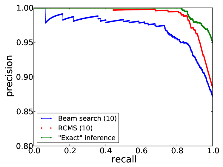
The precision-recall curve for each method is plotted in Figure 3; confidence is the probability the model assigns to the predicted output. Note that while beam search and RCMS achieve similar accuracies (precision at $R=1$) on the full test set ($87.1\%$ and $88.5\%$, respectively), RCMS is much better at separating out examples that are likely to be correct. The flat region in the precision-recall curve for beam search means that the model confidence and actual error probability are unrelated across that region.

As a result, there is a precision ceiling, where it is simply impossible to obtain high precision at any reasonable level of recall. To quantify this effect, note that the recall at $99\%$ precision for beam search is only $16\%$, while for RCMS it is $82\%$. For comparison, the recall for exact inference is only $4\%$ higher ($86\%$). Therefore, RCMS is nearly as effective as exact inference on this metric while requiring substantially fewer computational resources.

6 Learning with Indirect Supervision

The second symptom of lack of coverage is the inability to learn from indirect supervision. In this setting, we have an exponential family model $p_{\theta}(y,z\mid x)\propto\exp(\theta^{\top}\phi(x,y,z))$, where $x$ and $y$ are observed during training but $z$ is unobserved. The gradient of the (marginal) log-likelihood is:

$$\nabla\log p_{\theta}(y\mid x) =\mathbb{E}_{\hat{z}\sim p_{\theta}(z\mid x,y)}\left[\phi(x,y,\hat{z})\right]$$ (7)

$$\phantom{==}-\mathbb{E}_{\hat{y},\hat{z}\sim p_{\theta}(y,z\mid x)}\left[\phi(x,\hat{y},\hat{z})\right],$$

which is the difference between the expected features with respect to the target distribution $p_{\theta}(z\mid x,y)$ and the model distribution $p_{\theta}(y,z\mid x)$. In the fully supervised case, where we observe $z$, the target term is simply $\phi(x,y,z)$, which provides a clear training signal without any inference. With indirect supervision, even obtaining a training signal requires inference with respect to $p_{\theta}(z\mid x,y)$, which is generally intractable.

In the context of beam search, there are several strategies to inferring $z$ for computing gradients:

• Select-by-model: select beams based on $q_{\theta}^{i}(z\!\mid\!x)$, then re-weight at the end by $p_{\theta}(y\!\mid\!z,x)$. This only works if the weights are high for at least some “easy” examples, from which learning can then bootstrap.

• Select-by-target: select beams based on $q_{\theta}^{i}(z\!\mid\!x,y)$. Since $y$ is not available at test time, parameters $\theta$ learned conditioned on $y$ do not generalize well.

• Hybrid: take the union of beams based on both the model and target distributions.

• Forced decoding (Gorman et al., 2011): first train a simple model for which exact inference is tractable to infer the most likely $z$, conditioned on $x$ and $y$. Then simply fix $z$; this becomes a fully-supervised problem.

To understand the behavior of these methods, we used them all to train a model on the speech recognition dataset from Section 2. The model places $5$-gram indicator features on the output as well as on the alignments. We trained using AdaGrad with step size $\eta=0.2$ and $\delta=10^{-4}$. For each method, we set the beam size to $20$. For forced decoding, we used a bigram model with exact inference to impute $z$ at the beginning.

Figure 4: Left: character error rate (CER) of all beam search-based methods on the speech task, for $5$ passes of the training data; note that an empty output always has a CER of $1.0$. Middle: CER of forced decoding and RCMS over $5$ random permutations of the data; the solid line is the median. Right: exact-match accuracy over the same $5$ permutations.

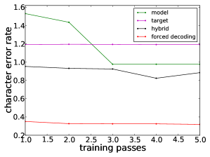
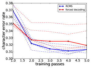
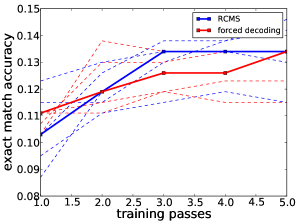
The results are shown in Figure 4. Select-by-model doesn’t learn at all: it only finds valid alignments for $2$ out of the $746$ training examples; for the rest, $p_{\theta}(y\mid z,x)$ is zero for all alignments considered, thus providing no signal for learning. Select-by-target quickly reaches high training accuracy, but generalizes extremely poorly because it doesn’t learn to keep the right answer on the beam. The hybrid approach does better but still not very well. The only method that learns effectively is forced decoding.

While forced decoding works well, it relies on the idea that a simple model can effectively determine $z$ given access to $x$ and $y$. This will not always be the case, so we would like methods that work well even without such a model. Reified context models provide a natural way of doing this: we simply compute $p_{\theta}(z\mid x,y)$ under the contexts selected by RCMS, and perform learning updates in the natural way.

To test RCMS, we trained it in the same way using $20$ contexts per position. Without any need for an initialization scheme, we obtain a model whose test accuracy is better than that of forced decoding (see Figures 4,4).

Decipherment: Unsupervised Learning.

We now turn our attention to an unsupervised problem: the decipherment task from Section 2. We model decipherment as a hidden Markov model (HMM): the hidden plain text evolves according to an $n$-th order Markov chain, and the cipher text is emitted based on a deterministic but unknown 1:1 substitution cipher (Ravi & Knight, 2009).

All the methods we described for speech recognition break down in the absence of any supervision except select-by-model. We therefore compare only three methods: select-by-model (beam search), RCMS, and exact inference. We trained a $1$st-order (bigram) HMM using all 3 methods, and a $2$nd-order (trigram) HMM using only beam search and RCMS, as exact inference was too slow (the vocabulary size is $500$). We used the given plain text to learn the transition probabilities, using absolute discounting (Ney et al., 1994) for smoothing. Then, we used EM to learn the transition probabilities; we used Laplace smoothing for these updates.

Figure 5: Results on the decipherment task. Left: accuracy for a fixed beam/context size as the model order varies; approximate inference with a $2$nd-order HMM using RCMS outperforms both beam search in the same model and exact inference in a simpler model. Right: effect of beam/context size on accuracy for the $2$nd-order HMM. RCMS is much more robust to changes in beam/context size.

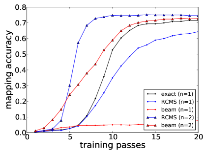
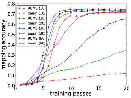
The results are shown in Figure 5. We measured performance by mapping accuracy: the fraction of unique symbols that are correctly mapped (Nuhn et al., 2013). First, we compared the overall accuracy of all methods, setting the beam size and context size both to $60$. We see that all $2$nd-order models outperform all $1$st-order models, and that beam search barely learns at all for the $1$st-order model.

Restricting attention to $2$nd-order models, we measure the effect of beam size and context size on accuracy, plotting learning curves for sizes of $10$, $20$, $30$, and $60$. In all cases, RCMS learns more quickly and converges to a more accurate solution than beam search. The shapes of the learning curves are also different: RCMS learns quickly after a few initial iterations, while beam search slowly accrues information at a roughly constant rate over time.

7 Refinement of Contexts During Training

When learning with indirect supervision and approximate inference, one intuition is that we can “bootstrap” by first learning from easy examples, and then using the information gained from these examples to make better inferences about the remaining ones (Liang et al., 2011). However, this can fail if there are insufficiently many easy examples (as in the speech task), if the examples are hard to identify, or if they differ statistically from the remaining examples.

We think of the above as “vertical bootstrapping”: using the full model on an increasing number of examples. RCMS instead performs “horizontal bootstrapping”: for each example, it selects a model (via the context sets) based on the information available. As training progresses, we expect these contexts to become increasingly fine as our parameters improve.

To measure this quantitatively, we define the length of a context $c_{i-1}$ to be the number of positions of $y_{1:i-1}$ that can be determined from $c_{i-1}$ (number of non-$\star$’s). We plot the average length (weighted by mass under $q_{\theta}^{i}$) as training progresses. The averages are updated every $50$ and $100$ training examples respectively for word and speech recognition. For decipherment, they are computed once for each full pass over the training data (since EM only updates the parameters once per pass).

Figure 6: Average context length vs. number of learning updates for the word recognition, speech, and decipherment tasks. For word and speech recognition we take a cumulative average (to reduce noise).

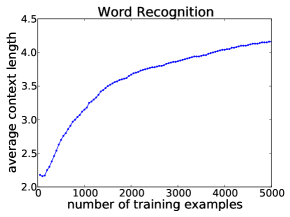
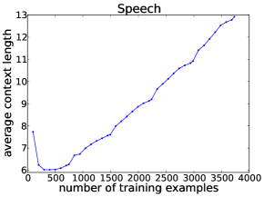
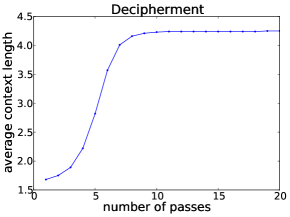
Figure 6 shows that the broad trend is an increase in the context length over time. For both the word and speech tasks, there is an initial overshoot at the beginning that is not present in the decipherment task; this is because the word and speech tasks are trained with stochastic gradient methods, which often overshoot and then correct in parameter space, while for decipherment we use the more stable EM algorithm.

Since we start by using coarse contexts and move to finer contexts by the end of training, RCMS can be thought of as a coarse-to-fine training procedure (Petrov & Charniak, 2011). However, instead of using a pre-defined, discrete set of models for initialization, we organically adapt the amount of context on a per-example basis.

8 Related work

Kulesza & Pereira (2007) first study the interaction between approximate inference and learning, showing that even in the fully supervised case approximate inference can be seriously detrimental; Finley & Joachims (2008) show that approximate inference algorithms which over-generate possible outputs interact best with learning; this further supports the need for coverage when learning.

Four major approaches have been taken to address the problem of learning with inexact inference. The first modifies the learning updates to account for the inference procedure, as in the max-violation perceptron and related algorithms (Huang et al., 2012; Zhang et al., 2013; Yu et al., 2013); reinforcement learning approaches to inference (Daumé III et al., 2009; Shi et al., 2015) also fit into this category. Another approach modifies the inference algorithm to obtain better coverage, as in coarse-to-fine inference (Petrov et al., 2006; Weiss et al., 2010), where simple models are used to direct the focus of more complex models. Pal et al. (2006) encourage coverage for beam search by adaptively increasing the beam size. A third approach is to use inference procedures with certificates of optimality, based on either duality gaps from convex programs (Sontag, 2010) or variational bounds (Xing et al., 2002; Wainwright et al., 2005).

Finally, another way of sidestepping the problems of approximate inference is to learn a model that is already tractable. While classical tractable model families based on low treewidth are often insufficiently expressive, more modern families have shown promise; for instance, sum-product networks (Poon & Domingos, 2011) can express models with high treewidth while still being tractable, and have achieved state-of-the-art results for some tasks. Other work includes exchangeable variable models (Niepert & Domingos, 2014) and mean-field networks (Li & Zemel, 2014).

Our method RCMS also attempts to define tractable model families, in our case, via a parsimonious choice of latent context variables, even though the actual distribution over $y_{1:L}$ may have arbitrarily high treewidth. We adaptively choose the model structure for each example at “run-time”, which distinguishes our approach from the aforementioned methods, though sum-product networks have some capacity for expressing adaptivity implicitly. We believe that such per-example adaptivity is important for obtaining good performance on challenging structured prediction tasks.

Certain smoothing techniques in natural language processing also interpolate between contexts of different order, such as absolute discounting (Ney et al., 1994) and Kneser-Ney smoothing Kneser & Ney (1995). However, in such cases all observed contexts are used in the model; to get the same tractability gains as we do, it would be necessary to adaptively sparsify the model for each example at run-time. Some Bayesian nonparametric approaches such as infinite contingent Bayesian networks (Milch et al., 2005) and hierarchical Pitman-Yor processes (Teh, 2006; Wood et al., 2009) also reason about contexts; again, such models do not lead to tractable inference.

9 Discussion

We have presented a new framework, reified context models, that reifies context as a random variable, thereby defining a family of expressive but tractable probability distributions. By adaptively choosing context sets at run-time, our RCMS method uses short contexts in regions of high uncertainty and long contexts in regions of low uncertainty, thereby reproducing the behavior of coarse-to-fine training methods in a more organic and fine-grained manner. In addition, because RCMS maintains full coverage of the space, it is able to break through the precision ceiling faced by beam search. Coverage also helps with training under indirect supervision, since we can better identify settings of latent variables that assign high likelihood to the data.

At a high level, our method provides a framework for structuring inference in terms of the contexts it considers; because the contexts are reified in the model, we can also support queries about how much probability mass lies in each context. These two properties together open up intriguing possibilities. For instance, one could imagine a multi-pass approach to inference where the first pass uses small context sets for each location, and later passes add additional contexts at locations where there is high uncertainty. By adaptively adding context only when it is needed, we could speed up inference by a potentially large amount.

Another direction of research is to extend our construction beyond a single left-to-right ordering. In principle, we can consider any collection of contexts that induce a graphical model with low treewidth, rather than only considering the factorization in (3). For problems such as image segmentation where the natural structure is a grid rather than a chain, such extensions may be necessary.

Finally, while we currently learn how much weight to assign to each context, we could go one step further and learn which contexts to propose and include in the context sets $\mathcal{C}_{i}$ (rather than relying on a fixed procedure as in the RCMS algorithm). Ideally, one could specify a large number of possible strategies for building context sets, and the best strategy to use for a given example would be learned from data. This would move us one step closer to being able to employ arbitrarily expressive models with the assurance of an automatic inference procedure that can take advantage of the expressivity in a reliable manner.

Appendix A Implementation Details

Recall that to implement the RCMS method, we need to perform the following steps:

1. Let $\tilde{\mathcal{C}}_{i}=\{c_{i-1}\times\{y_{i}\}\mid c_{i-1}\in\mathcal{C}_{i-1},y_{i}\in\mathcal{Y}_{i}\}$.

2. Compute what the mass of each element of $\tilde{\mathcal{C}}_{i}$ would be if we used $q_{\theta}^{i}$ as the model and $\tilde{\mathcal{C}}_{i}$ as the collection of contexts.

3. Let $\mathcal{C}_{i}$ be the $B$ elements of $\tilde{\mathcal{C}}_{i}$ with highest mass, together with the set $\mathcal{Y}_{1:i}$.

As in Section 4, each context in $\mathcal{C}_{i}$ can be represented by a string $s_{1:i}$, where $s_{j}\in\mathcal{Y}_{j}\cup\{\star\}$. We will also assume an arbitrary ordering on $\mathcal{Y}_{j}\cup\{\star\}$ that has $\star$ as its maximum element.

In addition, we use two datatypes: E (for “expand”), which keeps track of elements of $\tilde{\mathcal{C}}_{i}$, and M (for “merge”), which keeps track of elements of $\mathcal{C}_{i}$. More precisely, if $c_{i-1}$ is represented by an object $m_{i-1}$ of type M, then ${\texttt{E}}(m_{i-1},y_{i})$ represents $c_{i-1}\times\{y_{i}\}$; and ${\texttt{M}}({\texttt{E}}(m_{i-1},y_{i}))$ represents $c_{i-1}\times\{y_{i}\}$ as well, with the distinction that it is a member of $\mathcal{C}_{i}$ rather than $\tilde{\mathcal{C}_{i}}$. The distinction is important because we will also want to merge smaller contexts into objects of type M. For both E and M objects, we maintain a field $\operatorname{len}$, which is the length of the suffix of $y_{1:i}$ that is specified (e.g., if an object represents $\mathcal{Y}_{1:3}\times\{y_{4:5}\}$, then its $\operatorname{len}$ is $2$).

Throughout our algorithm, we will maintain $2$ invariants:

• $\tilde{\mathcal{C}}_{i}$ and $\mathcal{C}_{i}$ will be sorted lexicographically (e.g. based first on $s_{i}$, then $s_{i-1}$, etc.)

• A list $\widetilde{\operatorname{lcs}}_{i}$ of length $\operatorname{len}(\tilde{\mathcal{C}}_{i})$ is maintained, such that the longest common suffix of $\tilde{\mathcal{C}}_{i}[a]$ and $\tilde{\mathcal{C}}_{i}[b]$ is $\min_{c\in[a,b)}\widetilde{\operatorname{lcs}}_{i}[c]$. A similar list $\operatorname{lcs}_{i}$ is maintained for $\mathcal{C}_{i}$.

Step 1.

To perform step $1$ above, we just do:

  $\tilde{\mathcal{C}}_{i}=[]$

  for $j=0$ to $\operatorname{len}(\mathcal{Y}_{i})-1$ do

     for $k=0$ to $\operatorname{len}(\mathcal{C}_{i-1})-1$ do

        if $k+1<\operatorname{len}(\mathcal{C}_{i-1})$ then

           $\widetilde{\operatorname{lcs}}_{i}$.append($\operatorname{lcs}_{i-1}[k]+1$)

        else

           $\widetilde{\operatorname{lcs}}_{i}$.append($0$)

        end if

        $\tilde{\mathcal{C}}_{i}$.append(E($\mathcal{C}_{i}[k]$, $\mathcal{Y}_{i}[j]$))

     end for

  end for

The important observation is that if two sequences end in the same character, their $\operatorname{lcs}$ is one greater than the $\operatorname{lcs}$ of the remaining sequence without that character; and if they end in different characters, their $\operatorname{lcs}$ is $0$.

Each E keeps track of a forward score, defined as

$${\texttt{E}}(m,y).\mathrm{forward}=m.\mathrm{forward}\times\exp(\theta^{\top}\phi(m,y)).$$ (8)

Step 2.

For step $2$, we find the $B$ elements $\tilde{c}$ of $\tilde{\mathcal{C}}_{i}$ with the largest forward score; we set a flag $\tilde{c}.\mathrm{active}$ to true for each such $\tilde{c}$.

Step 3.

Step $3$ contains the main algorithm challenge, which is to efficiently merge each element of $\tilde{\mathcal{C}}_{i}$ into its least ancestor in $\mathcal{C}_{i}$. If we think of $\mathcal{C}_{i}$ as a tree (as in Figure 2), we can do this by essentially performing a depth-first-search of the tree. The DFS goes backwards in the lexicographic ordering, so we need to reverse the lists $\mathcal{C}_{i}$ and $\operatorname{lcs}_{i}$ at the end.

  $\rhd$ merge and update $\operatorname{lcs}$

  $\operatorname{stack}=[]$

  $\mathcal{C}_{i}=[]$

  $\operatorname{lcs}_{i}=[]$

  $l\leftarrow\infty$

  for $j=\operatorname{len}(\tilde{\mathcal{C}}_{i})-1$ to $0$ do

     $l\leftarrow\min(l,\widetilde{\operatorname{lcs}}_{i}[j])$

     while $l<\operatorname{stack}[-1].\operatorname{len}$ do

        $\rhd$ then current top of stack is not an ancestor of $\tilde{\mathcal{C}}_{i}[j]$

        $\operatorname{stack}$.pop()

     end while

     if $\tilde{\mathcal{C}}_{i}[j].\mathrm{active}$ then

        $m={\texttt{M}}(\tilde{\mathcal{C}}_{i}[j])$

        $\operatorname{lcs}_{i}$.append($l$)

        $\mathcal{C}_{i}$.append($m$)

        $\operatorname{stack}$.push($m$)

        $l\leftarrow\infty$

     else

        $\rhd$ merge $\tilde{\mathcal{C}}_{i}[j]$ into its least ancestor

        $\operatorname{stack}[-1].\operatorname{absorb}(\tilde{\mathcal{C}}_{i}[j])$

     end if

  end for

  $\operatorname{lcs}_{i}$.reverse()

  $\mathcal{C}_{i}$.reverse()

If $m\in\mathcal{C}_{i}$ has absorbed elements $e_{1},\ldots,e_{k}$, then we compute $m.\mathrm{forward}$ as $\sum_{j=1}^{k}e_{j}.\mathrm{forward}$.

After we have constructed $\mathcal{C}_{1},\ldots,\mathcal{C}_{i-1}$, we also need to send backward messages for inference. If $e\in\tilde{\mathcal{C}}_{i}$ is merged into $m\in\mathcal{C}_{i}$, then $e.\operatorname{backward}=m.\operatorname{backward}$. If $m\in\mathcal{C}_{i}$ expands to ${\texttt{E}}(m,y)$ for $y\in\mathcal{Y}_{i+1}$, then $m.\operatorname{backward}=\sum_{y\in\mathcal{Y}_{i+1}}{\texttt{E}}(m,y).\operatorname{backward}\times\exp(\theta^{\top}\phi(m,y))$. The (un-normalized) probability mass of an object is then simply the product of its forward and backward scores; we can compute the normalization constant by summing over $\mathcal{C}_{i}$.

In summary, our method can be coded in three steps; first, during the forward pass of inference, we:

1. Expand to $\tilde{\mathcal{C}}_{i}$ and construct $\widetilde{\operatorname{lcs}}_{i}$.

2. Sort by forward score and mark active nodes in $\tilde{\mathcal{C}}_{i}$ for inclusion in $\mathcal{C}_{i}$.

3. Merge each node in $\tilde{\mathcal{C}}_{i}$ into its least ancestor in $\mathcal{C}_{i}$, using a depth-first-search.

Finally, once all of the $\mathcal{C}_{i}$ are constructed, we perform the backward pass:

1. Propagate backward messages and compute the normalization constant.

Appendix B Further Details of Experimental Setup

We include here a few experimental details that did not fit into the main text. When training with AdaGrad, we performed several stochastic gradient updates in parallel, similar to the approach described in Recht et al. (2011) (although we parallelized even more aggressively at the expense of theoretical guarantees). We also used a randomized truncation scheme to round most small coordinates of the gradients to zero, which substantially reduces memory usage as well as concurrency overhead.

For decipherment, we used absolute discounting with discount $0.25$ and smoothing $0.01$, and Laplace smoothing with parameter $0.01$. For the $1$st-order model, beam search performs better if we use Laplace smoothing instead of absolute discounting (though still worse than RCMS). In order to maintain a uniform experimental setup, we excluded this result from the main text.

For the hybrid selection algorithm in the speech experiments, we take the union of the beams at every step (as opposed to computing two sets of beams separately and then taking a single union at the end).

Appendix C Additional Files

In the supplementary material, we also include the source code and datasets for the decipherment task. A README is included to explain how to run these experiments.

References

- Brooks et al. (2011) Brooks, Steve, Gelman, Andrew, Jones, Galin, and Meng, Xiao-Li. Handbook of Markov Chain Monte Carlo. CRC press, 2011.
- Cappé et al. (2007) Cappé, Olivier, Godsill, Simon J, and Moulines, Eric. An overview of existing methods and recent advances in sequential Monte Carlo. Proceedings of the IEEE, 95(5):899–924, 2007.
- Daumé III et al. (2009) Daumé III, Hal, Langford, John, and Marcu, Daniel. Search-based structured prediction. Machine learning, 75(3):297–325, 2009.
- Doucet & Johansen (2011) Doucet, Arnaud and Johansen, Adam M. A tutorial on particle filtering and smoothing: Fifteen years later. In Oxford Handbook of Nonlinear Filtering. Citeseer, 2011.
- Duchi et al. (2010) Duchi, J., Hazan, E., and Singer, Y. Adaptive subgradient methods for online learning and stochastic optimization. In Conference on Learning Theory (COLT), 2010.
- Finley & Joachims (2008) Finley, Thomas and Joachims, Thorsten. Training structural svms when exact inference is intractable. In Proceedings of the 25th international conference on Machine learning, pp. 304–311. ACM, 2008.
- Gorman et al. (2011) Gorman, Kyle, Howell, Jonathan, and Wagner, Michael. Prosodylab-aligner: A tool for forced alignment of laboratory speech. Canadian Acoustics, 39(3):192–193, 2011.
- Graff & Cieri (2003) Graff, David and Cieri, Christopher. English Gigaword LDC2003T05. Philadelphia: Linguistic Data Consortium, 2003. Web Download.
- Greenberg et al. (1996) Greenberg, Steven, Hollenback, Joy, and Ellis, Dan. Insights into spoken language gleaned from phonetic transcription of the switchboard corpus. In Proceedings of the International Conference on Spoken Language Processing, 1996.
- Huang et al. (2012) Huang, Liang, Fayong, Suphan, and Guo, Yang. Structured perceptron with inexact search. In Proceedings of the 2012 Conference of the North American Chapter of the Association for Computational Linguistics: Human Language Technologies, pp. 142–151. Association for Computational Linguistics, 2012.
- Kassel (1995) Kassel, Robert H. A comparison of approaches to on-line handwritten character recognition. PhD thesis, Massachusetts Institute of Technology, 1995.
- Kneser & Ney (1995) Kneser, Reinhard and Ney, Hermann. Improved backing-off for m-gram language modeling. In Acoustics, Speech, and Signal Processing, 1995. ICASSP-95., 1995 International Conference on, volume 1, pp. 181–184. IEEE, 1995.
- Koehn et al. (2003) Koehn, Philipp, Och, Franz Josef, and Marcu, Daniel. Statistical phrase-based translation. In Proceedings of the 2003 Conference of the North American Chapter of the Association for Computational Linguistics on Human Language Technology-Volume 1, pp. 48–54. Association for Computational Linguistics, 2003.
- Kulesza & Pereira (2007) Kulesza, Alex and Pereira, Fernando. Structured learning with approximate inference. In Advances in neural information processing systems, pp. 785–792, 2007.
- Li & Zemel (2014) Li, Yujia and Zemel, Richard. Mean-field networks. arXiv preprint arXiv:1410.5884, 2014.
- Liang et al. (2011) Liang, P., Jordan, M. I., and Klein, D. Learning dependency-based compositional semantics. In Association for Computational Linguistics (ACL), pp. 590–599, 2011.
- Milch et al. (2005) Milch, Brian, Marthi, Bhaskara, Sontag, David, Russell, Stuart, Ong, Daniel L, and Kolobov, Andrey. Approximate inference for infinite contingent bayesian networks. In Proc. 10th AISTATS, pp. 238–245, 2005.
- Ney et al. (1994) Ney, Hermann, Essen, Ute, and Kneser, Reinhard. On structuring probabilistic dependences in stochastic language modelling. Computer Speech & Language, 8(1):1–38, 1994.
- Niepert & Domingos (2014) Niepert, Mathias and Domingos, Pedro. Exchangeable variable models. arXiv preprint arXiv:1405.0501, 2014.
- Nuhn & Ney (2014) Nuhn, Malte and Ney, Hermann. Improved decipherment of homophonic ciphers. In Conference on Empirical Methods in Natural Language Processing, Doha, Qatar, October 2014.
- Nuhn et al. (2013) Nuhn, Malte, Schamper, Julian, and Ney, Hermann. Beam search for solving substitution ciphers. In Annual Meeting of the Assoc. for Computational Linguistics, pp. 1569–1576, Sofia, Bulgaria, August 2013. URL http://aclweb.org/anthology//P/P13/P13-1154.pdf.
- Pal et al. (2006) Pal, Chris, Sutton, Charles, and McCallum, Andrew. Sparse forward-backward using minimum divergence beams for fast training of conditional random fields. In IEEE International Conference on Acoustics, Speech and Signal Processing, volume 5, pp. V–V. IEEE, 2006.
- Petrov et al. (2006) Petrov, S., Barrett, L., Thibaux, R., and Klein, D. Learning accurate, compact, and interpretable tree annotation. In International Conference on Computational Linguistics and Association for Computational Linguistics (COLING/ACL), pp. 433–440, 2006.
- Petrov & Charniak (2011) Petrov, Slav and Charniak, Eugene. Coarse-to-fine natural language processing. Springer Science & Business Media, 2011.
- Poon & Domingos (2011) Poon, Hoifung and Domingos, Pedro. Sum-product networks: A new deep architecture. In Computer Vision Workshops (ICCV Workshops), 2011 IEEE International Conference on, pp. 689–690. IEEE, 2011.
- Ravi & Knight (2009) Ravi, Sujith and Knight, Kevin. Attacking letter substitution ciphers with integer programming. Cryptologia, 33(4):321–334, 2009. doi: 10.1080/01611190903030920. URL http://dx.doi.org/10.1080/01611190903030920.
- Recht et al. (2011) Recht, Benjamin, Re, Christopher, Wright, Stephen, and Niu, Feng. Hogwild: A lock-free approach to parallelizing stochastic gradient descent. In Advances in Neural Information Processing Systems, pp. 693–701, 2011.
- Shi et al. (2015) Shi, Tianlin, Steinhardt, Jacob, and Liang, Percy. Learning where to sample in structured prediction. 2015.
- Sontag (2010) Sontag, David Alexander. Approximate inference in graphical models using LP relaxations. PhD thesis, Massachusetts Institute of Technology, 2010.
- Steinhardt & Liang (2014) Steinhardt, Jacob and Liang, Percy. Filtering with abstract particles. In Proceedings of the 31st International Conference on Machine Learning (ICML-14), pp. 727–735, 2014.
- Teh (2006) Teh, Yee Whye. A hierarchical bayesian language model based on pitman-yor processes. In Proceedings of the 21st International Conference on Computational Linguistics and the 44th annual meeting of the Association for Computational Linguistics, pp. 985–992. Association for Computational Linguistics, 2006.
- Wainwright et al. (2005) Wainwright, Martin J, Jaakkola, Tommi S, and Willsky, Alan S. A new class of upper bounds on the log partition function. Information Theory, IEEE Transactions on, 51(7):2313–2335, 2005.
- Weiss et al. (2010) Weiss, David, Sapp, Benjamin, and Taskar, Ben. Sidestepping intractable inference with structured ensemble cascades. In Advances in Neural Information Processing Systems, pp. 2415–2423, 2010.
- Weiss et al. (2012) Weiss, David, Sapp, Benjamin, and Taskar, Ben. Structured prediction cascades. arXiv preprint arXiv:1208.3279, 2012.
- Wood et al. (2009) Wood, Frank, Archambeau, Cédric, Gasthaus, Jan, James, Lancelot, and Teh, Yee Whye. A stochastic memoizer for sequence data. In Proceedings of the 26th Annual International Conference on Machine Learning, pp. 1129–1136. ACM, 2009.
- Xing et al. (2002) Xing, Eric P, Jordan, Michael I, and Russell, Stuart. A generalized mean field algorithm for variational inference in exponential families. In Proceedings of the Nineteenth conference on Uncertainty in Artificial Intelligence, pp. 583–591. Morgan Kaufmann Publishers Inc., 2002.
- Yu et al. (2013) Yu, Heng, Huang, Liang, Mi, Haitao, and Zhao, Kai. Max-violation perceptron and forced decoding for scalable mt training. In EMNLP, pp. 1112–1123, 2013.
- Zhang et al. (2013) Zhang, Hao, Huang, Liang, Zhao, Kai, and McDonald, Ryan. Online learning for inexact hypergraph search. In Proceedings of EMNLP, 2013.
- Zhang et al. (2014) Zhang, Liyan, Kalashnikov, Dmitri V., and Mehrotra, Sharad. Context-assisted face clustering framework with human-in-the-loop. International Journal of Multimedia Information Retrieval, 3(2):69–88, 2014. ISSN 2192-6611. doi: 10.1007/s13735-014-0052-1. URL http://dx.doi.org/10.1007/s13735-014-0052-1.