Lattice QCD with 2+1 Flavors and Open Boundaries: First Results of the Baryon Spectrum

Abstract:

Based on CLS simulations with 2+1 flavors and open boundaries we present first results of the baryon spectrum. We report on the status of our effort related to these simulations and the chiral extrapolation to the physical point.

1 Introduction

As more computing power and better algorithms have become available over the years the precision in lattice QCD results becomes more and more relevant. In order to have small errors on lattice QCD results it is important to have good control over the systematics involved in lattice simulations. Besides large volumes, quark masses close to the physical point, and large statistics, the continuum limit plays a prominent role because of the so-called topological freezing problem [1, 2, 3]. As the lattice spacing is decreased and, hence, the continuum is approached it becomes more and more difficult for conventional simulation techniques to tunnel between topologically distinct gauge sectors during the simulation. As a result, one faces large autocorrelation times for simulations at lattice spacings smaller than about $0.05~{}\mathrm{fm}$ [4]. With the conventional approach large statistics and/or large spatial volumes would be necessary to obtain meaningful results. A quite different and new approach to reduce the large autocorrelation times for quantities which couple to those topological modes is based on the introduction of open boundary conditions [5] which are, in practice, imposed in the time direction. Topological objects can then flow in and out through the temporal boundary, and, in fact, it has turned out that this approach is computationally advantageous [6] with respect to an – otherwise necessary – increase in volume and/or statistics.

Therefore, the CLS collaboration [7] has started a major effort to generate gauge field configurations with open boundary conditions aiming at large statistics and volumes as well as pion masses close to the physical point in order to get good control over all systematics. There has been generated a relatively large set of ensembles quite recently using Wilson fermions with $2+1$ flavors [8]. We report on first measurements on some of these ensembles, in particular we focus on first results of the $\mathrm{SU}(3)$ octet baryon spectrum and also briefly address the scale setting, see Sec. 3 and Sec. 4, respectively. Before, we will start with a short presentation of some details about the simulations.

2 Simulation Details

run id	H101	H102	H105	C101	D100
$m_{\pi}\approx$	420 MeV	350 MeV	280 MeV	220 MeV	130 MeV
$m_{K}\approx$	420 MeV	440 MeV	460 MeV	470 MeV	480 MeV

Table 1: CLS ensembles at $\beta=3.4$. Note that the D100 ensemble has currently only low statistics and is not considered in the analysis presented in this contribution.

A non-perturbatively $\mathcal{O}(a)$-improved Wilson action with tree-level Symanzik improved gauge action and $2+1$ flavors has been employed. We have simulated at pion masses ranging from about $420~{}\mathrm{MeV}$ down to about $130~{}\mathrm{MeV}$ following the strategy adopted from the QCDSF collaboration [9] where the sum of bare quark masses is kept constant along the chiral trajectory. This strategy not only simplifies the tuning process of the simulations but also has the advantage that one can extrapolate, e.g., the combination $m_{K}^{2}+m_{\pi}^{2}/2$ rather precisely to the physical point as it turns out that in leading order chiral perturbation theory this combination is proportional to the sum of quark masses, $m_{K}^{2}+m_{\pi}^{2}/2\propto\mathrm{Tr}M\equiv\sum_{i}m_{i}$, and, in addition, the corrections to this relation stay small down to the physical point. As the scale $t_{0}$ is known to depend only weakly on the quark mass (see also the upper left plot in Fig. 3) we use the dimensionless combination $\phi_{4}=8t_{0}(m_{K}^{2}+m_{\pi}^{2}/2)$ and match our chiral trajectories with different lattice spacings at a single point along the symmetric line, i.e. we have fixed $\mathrm{Tr}M$, respectively $\sum_{i}1/\kappa_{i}$, for each lattice spacing to match our target estimate $\phi_{4}|_{m_{ud}=m_{s}}=1.15$ for $m_{ud}\equiv m_{u}=m_{d}=m_{s}$. Note that, at the physical point, we obtain $\phi_{4}^{\mathrm{p}hys}|_{m_{ud}=m_{s}}=1.117(38)$ with $m_{\pi}=134.8(3)~{}\mathrm{MeV}$ and $m_{K}=494.2(4)~{}\mathrm{MeV}$ from Ref. [10], and $\sqrt{8t_{0}}=0.4144(59)(37)~{}\mathrm{fm}$ from Ref. [11].

Figure 1: Effective mass plots of the nucleon. The horizontal length of the red bars in the plots indicate the fit range which was chosen to be $[10,18]$, the vertical position indicates the fitted mean value and the width corresponds to the fit error. Note that for the C101 ensemble ($m_{\pi}\approx 220~{}\mathrm{MeV}$) the statistics is smaller compared to the other ensembles.

Currently, we have generated ensembles at three different lattice gauge couplings with $\beta=6/g^{2}=3.4,3.55,3.7$. In the following we present preliminary data only for our ensembles at $\beta=3.4$ which corresponds to a lattice spacing $a\approx 0.086~{}\mathrm{fm}$. Note that also for $\beta=3.55,3.7$ other quantities have been presented at this conference [12, 13]. We have summarized the pion and kaon masses of the ensembles with $\beta=3.4$ in Tab. 1. Note that the D100 ensemble has currently only low statistics and is therefore not be taken into account in the analysis below. The lattice geometry for the ensembles H101, H102, and H105 is $32^{3}\times 96$ and for the C101 ensemble $48^{3}\times 96$ where the temporal extent of the lattices is typically larger compared to simulations with periodic boundary conditions due to the boundary effects specific to open boundary conditions. All ensembles have large spatial volumes $V_{s}=L^{3}$; for all ensembles $m_{\pi}L\gtrsim 4$ is satisfied. The HMC trajectory has length $\tau=2$ and for the ensembles under consideration more than 4000 Molecular Dynamic Units (MDUs) for each ensemble have been generated.

For the generation of gauge field configurations the openQCD package [14] has been used which has several algorithmic improvements built in. Besides the Hasenbusch trick [15], improved integrators [16], a multi-level integration scheme [17], and a deflated solver [18, 19], the twisted mass reweighting [6] should be pointed out because it is the first time that this technique has been applied within a larger set of simulations. In the light fermion part of the action a twisted mass term is introduced in order to push the eigenvalues of the Dirac operator away from zero and, hence, increase the stability of the HMC simulation.

To correct for the additional twisted mass term in the light quark action one has to reweight the observables. In addition, one also applies reweighting with respect to the strange quark action to account for errors coming from the rational approximation which is used to simulate the strange quark. The ensemble average of an observable $\left<O\right>=\frac{\left<WO\right>}{\left<W\right>}$ then includes the reweighting factor $W=W_{0}W_{1}$ with a light and strange reweighting factor $W_{0}$ and $W_{1}$, respectively. We found that these reweighting methods work quite nicely in practice, more details can be found in Ref. [8].

3 Baryon Spectrum

In this section we present first preliminary results on the baryon spectrum from simulations with open boundary conditions. In Sec. 3.1 we give some details about the computation of the spectrum, in Sec. 3.2 we discuss the chiral extrapolation of our results and also compare our findings to results from the literature.

Figure 2: Fits to the octet baryon masses of our preliminary data (right) compared to fits from Ref [9] based on data from Ref. [20] (left plot was taken from Ref [9]).

3.1 Computational Details

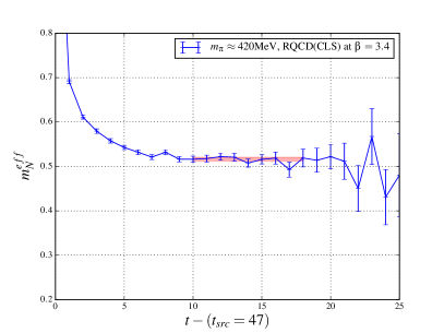
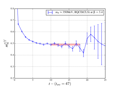
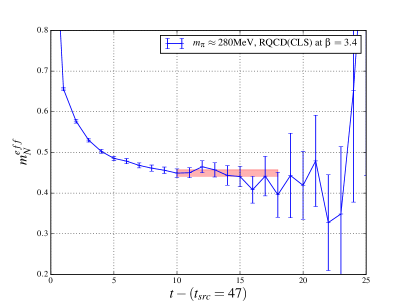
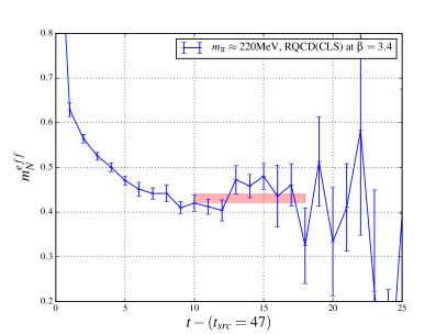
For the computation of the baryon spectrum we have used standard relativistic interpolators, e.g. for the nucleon we have used $I_{N}=\epsilon_{abc}u_{a}\left(u_{b}^{T}C\gamma_{5}d_{c}\right)$. The source position in temporal direction was always chosen to be at the center of the lattice, i.e. $t_{\mathrm{s}rc}=47$ where $t\in[0,\dots,95]$, the spatial source position was chosen randomly. We have been investigating smeared-smeared point-to-all correlators where we have used 100 steps of Wuppertal smearing on APE smeared gauge links for both the source and the sink. The fit range was chosen to be $t\in[10,18]$. For the ensembles H101, H102, and H105 all available 4000 MDUs for each ensemble have been analyzed, for the C101 ensemble 1000 MDUs have been considered so far. For the analysis a custom version of the CHROMA software package [21] has been developed where also the deflated solver [18] is used.

In Fig. 1 we show the effective mass of the nucleon for the ensembles under consideration. For the three ensembles where all configurations have been analyzed we observe a nice plateau while for the C101 ensemble one would expect that a less noisy plateau will develop once full statistics have become available. For $\Sigma$ and $\Xi$ the corresponding plots look similar. Note that it has turned out that for this preliminary analysis the smearing was not chosen optimally. We are currently running measurements with full statistics and optimized smearing and, hence, we expect to improve on the errors present in this study.

3.2 Chiral Extrapolation

In order to chirally extrapolate to the physical point we make use of $\mathrm{SU}(3)$ chiral perturbation theory. The octet baryon masses in terms of the pion and kaon masses to order $\mathcal{O}(p^{2})$ are given by [22],

$$\begin{split}m_{N}&=m_{0}-4b_{D}\dot{M}_{K}^{2}+4b_{F}\left(\dot{M}_{K}^{2}-\dot{M}_{\pi}^{2}\right)-2b_{0}\left(2\dot{M}_{K}^{2}+\dot{M}_{\pi}^{2}\right)+\cdots\,,\\ m_{\Lambda}&=m_{0}+\frac{4}{3}b_{D}\left(-4\dot{M}_{K}^{2}+\dot{M}_{\pi}^{2}\right)-2b_{0}\left(2\dot{M}_{K}^{2}+\dot{M}_{\pi}^{2}\right)+\cdots\,,\\ m_{\Sigma}&=m_{0}-4b_{D}\dot{M}_{\pi}^{2}-2b_{0}\left(2\dot{M}_{K}^{2}+\dot{M}_{\pi}^{2}\right)+\cdots\,,\\ m_{\Xi}&=m_{0}-4b_{D}\dot{M}_{K}^{2}-4b_{F}\left(\dot{M}_{K}^{2}-\dot{M}_{\pi}^{2}\right)-2b_{0}\left(2\dot{M}_{K}^{2}+\dot{M}_{\pi}^{2}\right)+\cdots\,.\end{split}$$ (1)

The average nucleon mass $X_{N}$ and average pion mass $X_{\pi}$ are defined by $X_{N}\equiv\left(m_{N}+m_{\Sigma}+m_{\Xi}\right)/3$ and $X_{\pi}^{2}\equiv\left(2m_{K}^{2}+m_{\pi}^{2}\right)/3$. In leading order chiral perturbation theory one finds,

$$X_{N}=m_{0}-2b_{0}\left(2\dot{M}_{K}^{2}+\dot{M}_{\pi}^{2}\right)+\cdots\,.$$ (2)

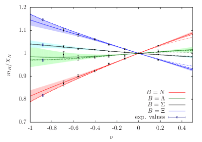
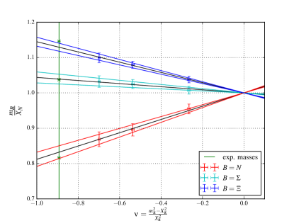
Since $2m_{K}^{2}+m_{\pi}^{2}$ is approximately constant along our chiral trajectory also the average nucleon mass stays constant to leading order along that line. We define the dimensionless quantity $\nu=\tfrac{m_{\pi}^{2}-X_{\pi}^{2}}{X_{\pi}^{2}}$ and plot the fits of our data to Eq. (1) in the right plot of Fig. 2. The errors on the masses come from uncorrelated fits where we have performed a jackknife analysis with binning. The left plot of Fig. 2 is taken from [20] where chiral fits have been performed to data from QCDSF [9]. Comparing those to our preliminary results we find nice agreement.

4 Scale Setting

To set the scale at a certain lattice coupling one would choose a dimensionful, (ideally) physical quantity and compare it to the lattice result. In order to do so we have to, in our case, chirally extrapolate to the physical point. For the following discussion we define as the physical point the value of $\kappa_{l}\equiv\kappa_{l}^{\mathrm{p}hys}$ at which the ratio of strange to light $\mathcal{O}(a)$-improved AWI quark masses takes its physical value of $27.46(44)$ [10]. The preliminary value of $\kappa_{l}^{\mathrm{p}hys}$ is taken from Ref. [23]. Note that $\kappa_{s}^{\mathrm{p}hys}$ is then determined by our definition of the chiral trajectory through $\mathrm{Tr}M=\mathrm{const}$. We remark that this definition is preliminary since we would hope to improve over the errors on that ratio given in Ref. [10] once the continuum limit can be taken.

Figure 3: Linear extrapolations of $\tfrac{t_{0}}{a^{2}}$, $\phi_{4}$, $\sqrt{t_{0}}X_{N}$, $\tfrac{X_{\pi}}{X_{N}}$ to the physical point (vertical red bars). The horizontal red bars indicate the corresponding experimental value including errors (or respectively the theoretical value including errors in the case of combinations involving $t_{0}$), the blue horizontal bar represent the respective lattice value with errors obtained by extrapolating the data to the physical point.

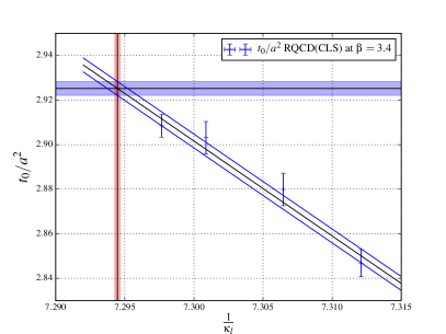
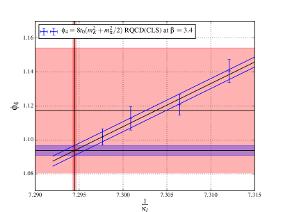
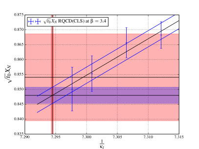
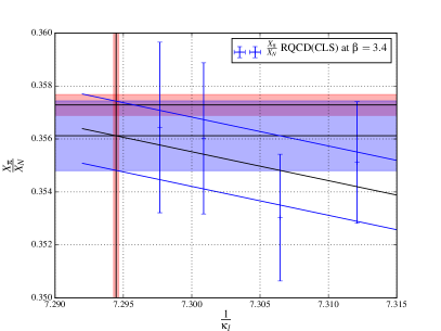
We first look at the chiral extrapolation of $\phi_{4}$, see the upper right plot in Fig. 3. Remember that $\phi_{4}$ has been used to match our chiral trajectory along the symmetric line. We can now ask whether our matching condition at that point results in an agreement at the physical point, i.e. $\phi_{4}$ obtains its physical value at the physical point which is actually what is desired. Since $m_{K}^{2}+m_{\pi}^{2}/2$ is constant to leading order along that trajectory and in addition $t_{0}$ is also only weakly dependent on the quark mass (see upper left plot in Fig. 3) we do not expect a strong quark mass dependence of $\phi_{4}$, in fact this is evident from the upper right plot of Fig. 3 and we find agreement of $\phi_{4}$ at the physical point with its physical value within errors. Up to cutoff effects, this means that we have indeed chosen the correct value of $\mathrm{Tr}M$ for our chiral trajectory. However, since we do not know much about the cutoff dependence at the present stage, it is interesting to compare how different quantities match at the physical point because different quantities could have very different cutoff dependence. Let us take a closer look at $\sqrt{t_{0}}X_{N}$ and $\tfrac{X_{\pi}}{X_{N}}$. The chiral extrapolations are shown in the lower plots of Fig. 3. Within errors we find again agreement for those quantities at the physical point with the corresponding physical values. Again we would conclude that we have chosen the correct value of $\mathrm{Tr}M$ for our chiral trajectory, and, in addition, the cutoff effects seem to be small. Note, however, that without knowing the explicit cutoff dependence of the quantities under investigation it is not really possible to disentangle cutoff effects and effects stemming from a mistuning of our chiral trajectory, i.e. a wrong value of $\mathrm{Tr}M$. This will be clarified by a future study of our ensembles at different lattice spacings which will also enable an independent scale setting.

We remark that the conclusions we have drawn above, of course, depend on the actual value and error on $t_{0}$ which is a result from a lattice study [11] as $t_{0}$ is not experimentally accessible. We therefore also plan to extract $t_{0}$ from our simulations and once the continuum limit can be performed we expect to deliver an independent cross-check on that quantity.

Finally, coming back to the issue of scale setting, we remark that all quantities discussed in this section can be used for scale setting. As we have found that all these quantities agree well at the physical point with their corresponding physical value it is evident that the lattice spacings extracted by the quantities investigated here will results in similar values. As our results are still preliminary we will refrain from quoting numbers but will return to this topic in a different publication.

5 Summary and Outlook

We have presented first results on the baryon octet spectrum from lattice simulations with $2+1$ flavors and open boundaries which has been generated within the CLS collaboration. Using leading order chiral perturbation theory we have chirally extrapolated results down to the physical point for $N,\Sigma,\Xi$ at pion masses ranging from $m_{\pi}\approx 220-420~{}\mathrm{MeV}$ at a lattice spacing $a\approx 0.086~{}\mathrm{fm}$. We have found nice agreement with the literature. In addition, we have extrapolated $\tfrac{t_{0}}{a^{2}}$, $\phi_{4}$, $\sqrt{t_{0}}X_{N}$, $\tfrac{X_{\pi}}{X_{n}}$ to the physical point and have checked that $\phi_{4}$, which is used to match our chiral trajectories, agrees at this point with its physical value. Furthermore, we have found that $\sqrt{t_{0}}X_{N}$ and $\tfrac{X_{\pi}}{X_{n}}$ also agree with their corresponding physical values at this point suggesting that cutoff effects may be small and that the chiral trajectory has been chosen appropriate. A more detailed analysis including cutoff effects will follow in the future.

References

- [1] L. Del Debbio, H. Panagopoulos, and E. Vicari, theta dependence of SU(N) gauge theories, JHEP 0208 (2002) 044, [hep-th/0204125].
- [2] C. Bernard, T. A. DeGrand, A. Hasenfratz, C. E. Detar, J. Osborn, et al., Topological susceptibility with the improved Asqtad action, Phys.Rev. D68 (2003) 114501, [hep-lat/0308019].
- [3] S. Schaefer, R. Sommer, and F. Virotta, Critical slowing down and error analysis in lattice QCD simulations, Nucl.Phys. B845 (2011) 93–119, [arXiv:1009.5228].
- [4] M. Bruno, S. Schaefer, and R. Sommer, Topological susceptibility and the sampling of field space in Nf = 2 lattice QCD simulations, JHEP 1408 (2014) 150, [arXiv:1406.5363].
- [5] M. Lüscher and S. Schaefer, Lattice QCD without topology barriers, JHEP 1107 (2011) 036, [arXiv:1105.4749].
- [6] M. Lüscher and S. Schaefer, Lattice QCD with open boundary conditions and twisted-mass reweighting, Comput.Phys.Commun. 184 (2013) 519–528, [arXiv:1206.2809].
- [7] Coordinated Lattice Simulations (CLS), https://wiki-zeuthen.desy.de/CLS/CLS
- [8] M. Bruno, D. Djukanovic, G. P. Engel, A. Francis, G. Herdoiza, et al., Simulation of QCD with N 2 1 flavors of non-perturbatively improved Wilson fermions, JHEP 1502 (2015) 043, [arXiv:1411.3982].
- [9] W. Bietenholz, V. Bornyakov, M. Göckeler, R. Horsley, W. Lockhart, et al., Flavour blindness and patterns of flavour symmetry breaking in lattice simulations of up, down and strange quarks, Phys.Rev. D84 (2011) 054509, [arXiv:1102.5300].
- [10] S. Aoki, Y. Aoki, C. Bernard, T. Blum, G. Colangelo, et al., Review of lattice results concerning low-energy particle physics, Eur.Phys.J. C74 (2014), no. 9 2890, [arXiv:1310.8555].
- [11] S. Borsanyi, S. Durr, Z. Fodor, C. Hoelbling, S. D. Katz, et al., High-precision scale setting in lattice QCD, JHEP 1209 (2012) 010, [arXiv:1203.4469].
- [12] M. Bruno, On the extraction of spectral quantities with open boundary conditions, \posPos(LATTICE2014)089
- [13] P. Korcyl, The CLS 2+1 flavor simulations, \posPoS(LATTICE2014)029
- [14] http://luscher.web.cern.ch/luscher/openQCD/.
- [15] M. Hasenbusch, Speeding up the Hybrid-Monte-Carlo algorithm for dynamical fermions, Phys. Lett. B519 (2001) 177–182, [hep-lat/0107019].
- [16] I. P. Omelyan, I. M. Mryglod, and R. Folk, Symplectic analytically integrable decomposition algorithms: classification, derivation, and application to molecular dynamics, quantum and celestial mechanics simulations, Computer Physics Communications 151 (2003), no. 3 272 – 314.
- [17] J. Sexton and D. Weingarten, Hamiltonian evolution for the hybrid Monte Carlo algorithm, Nucl.Phys. B380 (1992) 665–678.
- [18] M. Lüscher, Deflation acceleration of lattice QCD simulations, JHEP 0712 (2007) 011, [arXiv:0710.5417].
- [19] A. Frommer, K. Kahl, S. Krieg, B. Leder, and M. Rottmann, Adaptive Aggregation Based Domain Decomposition Multigrid for the Lattice Wilson Dirac Operator, SIAM J.Sci.Comput. 36 (2014) A1581–A1608, [arXiv:1303.1377].
- [20] P. C. Bruns, L. Greil, and A. Schäfer, Chiral extrapolation of baryon mass ratios, Phys.Rev. D87 (2013), no. 5 054021, [arXiv:1209.0980].
- [21] R. G. Edwards and B. Joo, The Chroma software system for lattice QCD, Nucl.Phys.Proc.Suppl. 140 (2005) 832, [hep-lat/0409003].
- [22] V. Bernard, N. Kaiser, and U. G. Meissner, Critical analysis of baryon masses and sigma terms in heavy baryon chiral perturbation theory, Z.Phys. C60 (1993) 111–120, [hep-ph/9303311].
- [23] G. Bali, E. E. Scholz, J. Simeth, W.S., in preparation