Visualizing Object Detection Features

Abstract

We introduce algorithms to visualize feature spaces used by object detectors. Our method works by inverting a visual feature back to multiple natural images. We found that these visualizations allow us to analyze object detection systems in new ways and gain new insight into the detector’s failures. For example, when we visualize the features for high scoring false alarms, we discovered that, although they are clearly wrong in image space, they do look deceptively similar to true positives in feature space. This result suggests that many of these false alarms are caused by our choice of feature space, and supports that creating a better learning algorithm or building bigger datasets is unlikely to correct these errors. By visualizing feature spaces, we can gain a more intuitive understanding of recognition systems.

1 Introduction

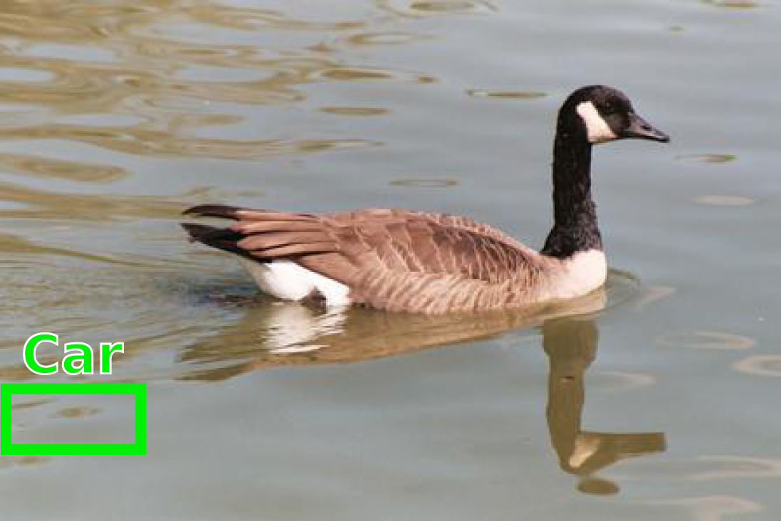
Figure 2 shows a high scoring detection from an object detector with HOG features and a linear SVM classifier trained on a large database of images. Why does this detector think that sea water looks like a car?

Figure 1: An image from PASCAL and a high scoring car detection from DPM (Felzenszwalb et al, 2010b). Why did the detector fail?

Figure 2: We show the crop for the false car detection from Figure 2. On the right, we show our visualization of the HOG features for the same patch. Our visualization reveals that this false alarm actually looks like a car in HOG space.

Figure 3: We visualize some high scoring detections from the deformable parts model (Felzenszwalb et al, 2010b) for person, chair, and car. Can you guess which are false alarms? Take a minute to study this figure, then see Figure 23 for the corresponding RGB patches.

Unfortunately, computer vision researchers are often unable to explain the failures of object detection systems. Some researchers blame the features, others the training set, and even more the learning algorithm. Yet, if we wish to build the next generation of object detectors, it seems crucial to understand the failures of our current detectors.

In this paper, we introduce a tool to explain some of the failures of object detection systems. We present algorithms to visualize the feature spaces of object detectors. Since features are too high dimensional for humans to directly inspect, our visualization algorithms work by inverting features back to natural images. We found that these inversions provide an intuitive visualization of the feature spaces used by object detectors.

Figure 2 shows the output from our visualization algorithm on the features for the false car detection. This visualization reveals that, while there are clearly no cars in the original image, there is a car hiding in the HOG descriptor. HOG features see a slightly different visual world than what we see, and by visualizing this space, we can gain a more intuitive understanding of our object detectors.

Figure 3 inverts more top detections on PASCAL for a few categories. Can you guess which are false alarms? Take a minute to study the figure since the next sentence might ruin the surprise. Although every visualization looks like a true positive, all of these detections are actually false alarms. Consequently, even with a better learning algorithm or more data, these false alarms will likely persist. In other words, the features are responsible for these failures.

Figure 4: Since there are many images that map to similar features, our method recovers multiple images that are diverse in image space, but match closely in feature space.

The primary contribution of this paper is a general algorithm for visualizing features used in object detection. We present a method that inverts visual features back to images, and show experiments for two standard features in object detection, HOG and activations from CNNs. Since there are many images that can produce equivalent feature descriptors, our method moreover recovers multiple images that are perceptually different in image space, but map to similar feature vectors, illustrated in Figure 4.

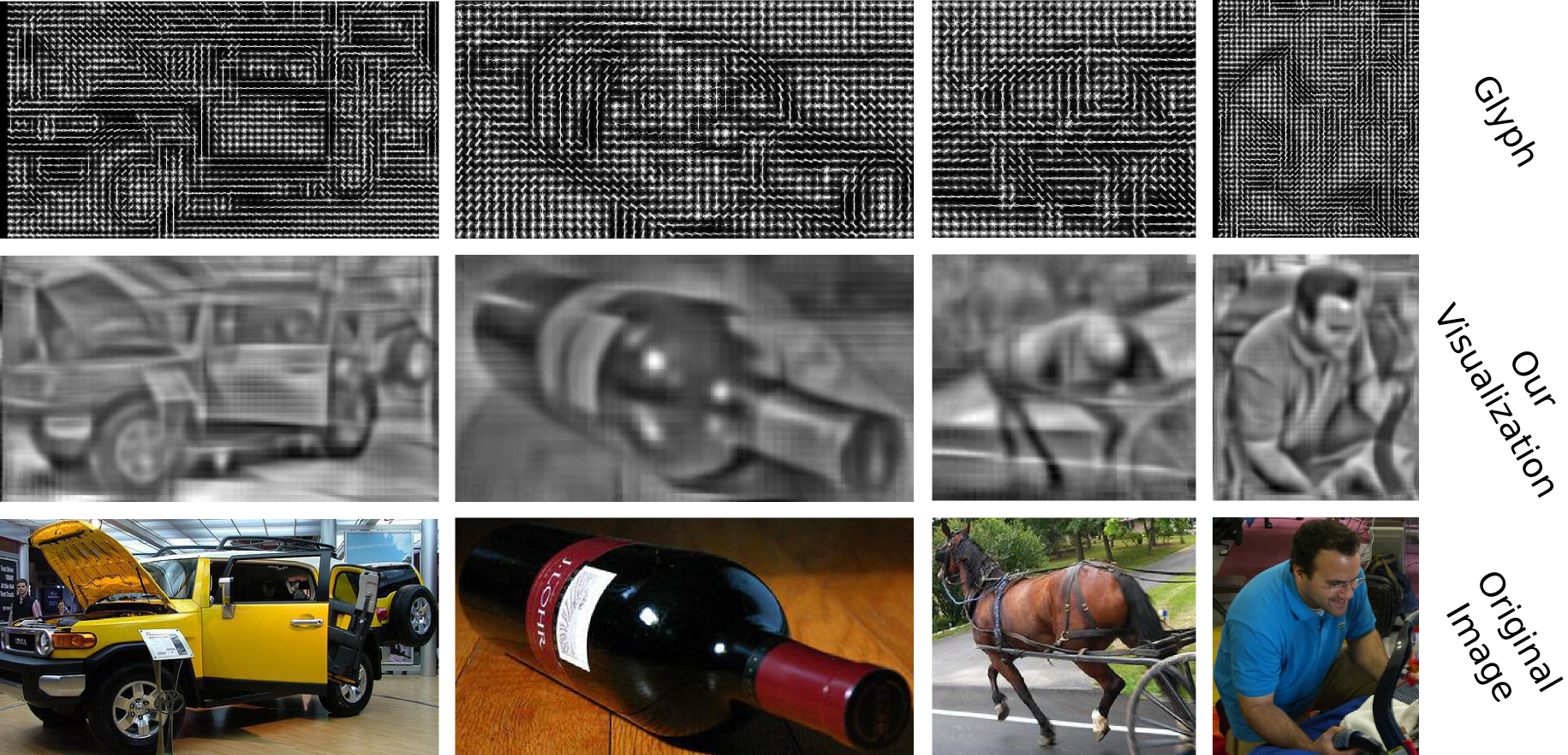
The remainder of this paper presents and analyzes our visualization algorithm. We first review a growing body of work in feature visualization for both handcrafted features and learned representations. We evaluate our inversions with both automatic benchmarks and a large human study, and we found our visualizations are perceptually more accurate at representing the content of a HOG feature than standard methods; see Figure 5 for a comparison between our visualization and HOG glyphs. We then use our visualizations to inspect the behaviors of object detection systems and analyze their features. Since we hope our visualizations will be useful to other researchers, our final contribution is a public feature visualization toolbox.

2 Related Work

Our visualization algorithms are part of an actively growing body of work in feature inversion. Oliva and Torralba (2001), in early work, described a simple iterative procedure to recover images given gist descriptors. Weinzaepfel et al (2011) were the first to reconstruct an image given its keypoint SIFT descriptors (Lowe, 1999). Their approach obtains compelling reconstructions using a nearest neighbor based approach on a massive database. d’Angelo et al (2012) then developed an algorithm to reconstruct images given only LBP features (Calonder et al, 2010; Alahi et al, 2012). Their method analytically solves for the inverse image and does not require a dataset. Kato and Harada (2014) posed feature inversion as a jigsaw puzzle problem to invert bags of visual words.

Figure 5: In this paper, we present algorithms to visualize features. Our visualizations are more perceptually intuitive for humans to understand.

Since visual representations that are learned can be difficult to interpret, there has been recent work to visualize and understand learned features. Zeiler and Fergus (2013) present a method to visualize activations from a convolutional neural network. In related work, Simonyan et al (2013) visualize class appearance models and their activations for deep networks. Girshick et al (2013) proposed to visualize convolutional neural networks by finding images that activate a specific feature. Mahendran and Vedaldi (2014) describe a general method for inverting visual features from CNNs by incorporating natural image priors.

While these methods are good at reconstructing and visualizing images from their respective features, our visualization algorithms have some advantages. Firstly, while most methods are tailored for specific features, the visualization algorithms we propose are feature independent. Since we cast feature inversion as a machine learning problem, our algorithms can be used to visualize any feature. In this paper, we focus on features for object detection, and we use the same algorithm to invert both HOG and CNN features. Secondly, our algorithms are fast: our best algorithm can invert features in under a second on a desktop computer, enabling interactive visualization, which we believe is important for real-time debugging of vision systems. Finally, our algorithm explicitly optimizes for multiple inversions that are diverse in image space, yet match in feature space.

Our method builds upon work that uses a pair of dictionaries with a coupled representation for super resolution (Yang et al, 2010; Wang et al, 2012) and image synthesis (Huang and Wang, 2013). We extend these methods to show that similar approaches can visualize features as well. Moreover, we incorporate novel terms that encourage diversity in the reconstructed image in order to recover multiple images from a single feature.

Feature visualizations have many applications in computer vision. The computer vision community has been using these visualization largely to understand object recognition systems so as to reveal information encoded by features (Zhang et al, 2014; Sadeghi and Forsyth, 2013), interpret transformations in feature space (Chen and Grauman, 2014), studying diverse images with similar features (Tatu et al, 2011; Lenc and Vedaldi, 2014), find security failures in machine learning systems (Biggio et al, 2012; Weinzaepfel et al, 2011), and fix problems in convolutional neural networks (Zeiler and Fergus, 2013; Simonyan et al, 2013; Bruckner, 2014). With many applications, feature visualizations are an important tool for the computer vision researcher.

Visualizations enable analysis that complement a recent line of papers that provide tools to diagnose object recognition systems, which we briefly review here. Parikh and Zitnick (2011, 2010) introduced a new paradigm for human debugging of object detectors, an idea that we adopt in our experiments. Hoiem et al (2012) performed a large study analyzing the errors that object detectors make. Divvala et al (2012) analyze part-based detectors to determine which components of object detection systems have the most impact on performance. Liu and Wang (2012) designed algorithms to highlight which image regions contribute the most to a classifier’s confidence. Zhu et al (2012) try to determine whether we have reached Bayes risk for HOG. The tools in this paper enable an alternative mode to analyze object detectors through visualizations. By putting on ‘HOG glasses’ and visualizing the world according to the features, we are able to gain a better understanding of the failures and behaviors of our object detection systems.

3 Inverting Visual Features

We now describe our feature inversion method. Let $x_{0}\in\mathbb{R}^{P}$ be a natural RGB image and $\phi=f(x_{0})\in\mathbb{R}^{Q}$ be its corresponding feature descriptor. Since features are many-to-one functions, our goal is to invert the features $\phi$ by recovering a set of images $\mathcal{X}=\{x_{1},\ldots,x_{N}\}$ that all map to the original feature descriptor.

We compute this inversion set $\mathcal{X}$ by solving an optimization problem. We wish to find several $x_{i}$ that minimize their reconstruction error in feature space $\left|\left|f(x_{i})-\phi\right|\right|_{2}^{2}$ while simultaneously appearing diverse in image space. We write this optimization as:

$$\mathcal{X}=\operatorname*{argmin}_{x,\xi} \sum_{i=1}^{N}\left|\left|f(x_{i})-\phi\right|\right|_{2}^{2}+\gamma\sum_{j<i}\xi_{ij}$$ (1)

s.t. $$0\leq S_{A}(x_{i},x_{j})\leq\xi_{ij}\;\forall_{ij}$$

The first term of this objective favors images that match in feature space and the slack variables $\xi_{ij}$ penalize pairs of images that are too similar to each other in image space where $S_{A}(x_{i},x_{j})$ is the similarity cost, parametrized by $A$, between inversions $x_{i}$ and $x_{j}$. A high similarity cost intuitively means that $x_{i}$ and $x_{j}$ look similar and should be penalized. The hyperparameter $\gamma\in\mathbb{R}$ controls the strength of the similarity cost. By increasing $\gamma$, the inversions will look more different, at the expense of matching less in feature space.

3.1 Similarity Costs

There are a variety of similarity costs that we could use. In this work, we use costs of the form:

$$S_{A}(x_{i},x_{j})=(x_{i}^{T}Ax_{j})^{2}$$ (2)

where $A\in\mathbb{R}^{P\times P}$ is an affinity matrix. Since we are interested in images that are diverse and not negatives of each other, we square $x_{i}^{T}Ax_{j}$. The identity affinity matrix, i.e. $A=I$, corresponds to comparing inversions directly in the color space. However, more metrics are also possible, which we describe now.

Edges: We can design $A$ to favor inversions that differ in edges. Let $A=C^{T}C$ where $C\in\mathbb{R}^{2P\times P}$. The first $P$ rows of $C$ correspond to the convolution with the vertical edge filters $\left[\begin{smallmatrix}-1&0&1\end{smallmatrix}\right]$ and similarly the second $P$ rows are for the horizontal edge filters $\left[\begin{smallmatrix}-1&0&1\end{smallmatrix}\right]^{T}$.

Color: We can also encourage the inversions to differ only in colors. Let $A=C^{T}C$ where $C\in\mathbb{R}^{3\times P}$ is a matrix that averages each color channel such that $Cx\in\mathbb{R}^{3}$ is the average RGB color.

Spatial: We can force the inversions to only differ in certain spatial regions. Let $A=C^{T}C$ where $C\in\mathbb{R}^{P\times P}$ is a binary diagonal matrix. A spatial region of $x$ will be only encouraged to be diverse if its corresponding element on the diagonal of $C$ is $1$. Note we can combine spatial similarity costs with both color and edge costs to encourage color and edge diversity in only certain spatial regions as well.

3.2 Optimization

Unfortunately, optimizing equation 1 efficiently is challenging because it is not convex. Instead, we will make two modifications to solve an approximation:

Figure 6: Inverting features using a paired dictionary. We first project the feature vector on to a feature basis. By jointly learning a coupled basis of features and natural images, we can transfer coefficients estimated from features to the image basis to recover the natural image.

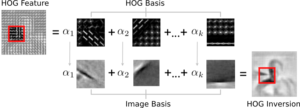
Modification 1: Since the first term of the objective depends on the feature function $f(\cdot)$, which is often not convex nor differentiable, efficient optimization is difficult. Consequently, we approximate an image $x_{i}$ and its features $\phi=f(x_{i})$ with a paired, over-complete basis to make the objective convex. Suppose we represent an image $x_{i}\in\mathbb{R}^{P}$ and its feature $\phi\in\mathbb{R}^{Q}$ in a natural image basis $U\in\mathbb{R}^{P\times K}$ and a feature space basis $V\in\mathbb{R}^{Q\times K}$ respectively. We can estimate $U$ and $V$ such that images and features can be encoded in their respective bases but with shared coefficients $\alpha\in\mathbb{R}^{K}$:

$$x_{0}=U\alpha\quad\textrm{and}\quad\phi=V\alpha$$ (3)

If $U$ and $V$ have this paired representation, then we can invert features by estimating an $\alpha$ that reconstructs the feature well. See Figure 6 for a graphical representation of the paired dictionaries.

Modification 2: However, the objective is still not convex when there are multiple outputs. We approach solving equation 1 sub-optimally using a greedy approach. Suppose we already computed the first $i-1$ inversions, $\{x_{1},\ldots,x_{i-1}\}$. We then seek the inversion $x_{i}$ that is only different from the previous inversions, but still matches $\phi$.

Taking these approximations into account, we solve for the inversion $x_{i}$ with the optimization:

$$\alpha_{i}^{*}=\operatorname*{argmin}_{\alpha_{i},\xi}||V\alpha_{i}-\phi||_{2}^{2}+\lambda||\alpha_{i}||_{1}+\gamma\sum_{j=1}^{i-1}\xi_{j}$$ (4)

$$\textrm{s.t.}\quad S_{A}(U\alpha_{i},x_{j})\leq\xi_{j}$$

where there is a sparsity prior on $\alpha_{i}$ parameterized by $\lambda\in\mathbb{R}$. After estimating $\alpha_{i}^{*}$, the inversion is $x_{i}=U\alpha_{i}^{*}$.

Figure 7: Some pairs of dictionaries for $U$ and $V$. The left of every pair is the gray scale dictionary element and the right is the positive components elements in the HOG dictionary. Notice the correlation between dictionaries.

The similarity costs can be seen as adding a weighted Tikhonov regularization ($\ell 2$ norm) on $\alpha_{i}$ because

$$S_{A}(U\alpha_{i},x_{j})=\alpha_{i}^{T}B\alpha_{i}\quad\textrm{where}\quad B=U^{T}A^{T}x_{j}^{T}x_{j}AU$$

Since this is combined with lasso, the optimization behaves as an elastic net (Zou and Hastie, 2005). Note that if we remove the slack variables ($\gamma=0$), our method reduces to (Vondrick et al, 2013) and only produces one inversion.

As the similarity costs are in the form of equation 2, we can absorb $S_{A}(x;x_{j})$ into the $\ell 2$ norm of equation 4. This allows us to efficiently optimize equation 4 using an off-the-shelf sparse coding solver. We use SPAMS (Mairal et al, 2009) in our experiments. The optimization typically takes a few seconds to produce each inversion on a desktop computer.

3.3 Learning

Figure 8: We found that averaging the images of top detections from an exemplar LDA detector provide one method to invert HOG features.

The bases $U$ and $V$ can be learned such that they have paired coefficients. We first extract millions of image patches $x_{0}^{(i)}$ and their corresponding features $\phi^{(i)}$ from a large database. Then, we can solve a dictionary learning problem similar to sparse coding, but with paired dictionaries:

$$\operatorname*{argmin}_{U,V,\alpha} \sum_{i}||x_{0}^{(i)}-U\alpha_{i}||_{2}^{2}+||\phi^{(i)}-V\alpha_{i}||_{2}^{2}+\lambda||\alpha_{i}||_{1}$$ (5)

s.t. $$||U||_{2}^{2}\leq\psi_{1},\;||V||_{2}^{2}\leq\psi_{2}\$$

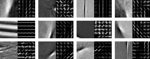
for some hyperparameters $\psi_{1}\in\mathbb{R}$ and $\psi_{2}\in\mathbb{R}$. We optimize the above with SPAMS (Mairal et al, 2009). Optimization typically took a few hours, and only needs to be performed once for a fixed feature. See Figure 7 for a visualization of the learned dictionary pairs.

4 Baseline Feature Inversion Methods

In order to evaluate our method, we also developed several baselines that we use for comparison. We first describe three baselines for single feature inversion, then discuss two baselines for multiple feature inversion.

4.1 Exemplar LDA (ELDA)

Consider the top detections for the exemplar object detector (Hariharan et al, 2012; Malisiewicz et al, 2011) for a few images shown in Figure 8. Although all top detections are false positives, notice that each detection captures some statistics about the query. Even though the detections are wrong, if we squint, we can see parts of the original object appear in each detection.

We use this observation to produce our first baseline. Suppose we wish to invert feature $\phi$. We first train an exemplar LDA detector (Hariharan et al, 2012) for this query, $w=\Sigma^{-1}(y-\mu)$ where $\Sigma$ and $\mu$ are parameters estimated with a large dataset. We then score $w$ against every sliding window in this database. The feature inverse is the average of the top $K$ detections in RGB space: $f^{-1}(\phi)=\frac{1}{K}\sum_{i=1}^{K}z_{i}$ where $z_{i}$ is an image of a top detection.

This method, although simple, produces reasonable reconstructions, even when the database does not contain the category of the feature template. However, it is computationally expensive since it requires running an object detector across a large database. Note that a similar nearest neighbor method is used in brain research to visualize what a person might be seeing (Nishimoto et al, 2011).

4.2 Ridge Regression

We describe a fast, parametric inversion baseline based off ridge regression. Let $X\in\mathbb{R}^{P}$ be a random variable representing a gray scale image and $\Phi\in\mathbb{R}^{Q}$ be a random variable of its corresponding feature. We define these random variables to be normally distributed on a $P+Q$-variate Gaussian $P(X,\Phi)\sim\mathcal{N}(\mu,\Sigma)$ with parameters $\mu=\left[\begin{smallmatrix}\mu_{X}&\mu_{\Phi}\end{smallmatrix}\right]$ and $\Sigma=\left[\begin{smallmatrix}\Sigma_{XX}&\Sigma_{X\Phi}\\ \Sigma_{X\Phi}^{T}&\Sigma_{Y\Phi}\end{smallmatrix}\right]$. In order to invert a feature $y$, we calculate the most likely image from the conditional Gaussian distribution $P(X|\Phi=\phi)$:

$$f^{-1}(y) =\operatorname*{argmax}_{x\in\mathbb{R}^{D}}P(X=x|\Phi=\phi)$$ (6)

It is well known that a Gaussian distribution have a closed form conditional mode:

$$f^{-1}(y)=\Sigma_{X\Phi}\Sigma_{\Phi\Phi}^{-1}(y-\mu_{\Phi})+\mu_{X}$$ (7)

Under this inversion algorithm, any feature can be inverted by a single matrix multiplication, allowing for inversion in under a second.

We estimate $\mu$ and $\Sigma$ on a large database. In practice, $\Sigma$ is not positive definite; we add a small uniform prior (i.e., $\hat{\Sigma}=\Sigma+\lambda I$) so $\Sigma$ can be inverted. Since we wish to invert any feature, we assume that $P(X,\Phi)$ is stationary (Hariharan et al, 2012), allowing us to efficiently learn the covariance across massive datasets. For features with varying spatial dimensions, we invert a feature by marginalizing out unused dimensions.

4.3 Direct Optimization

We now provide a baseline that attempts to find images that, when we compute features on it, sufficiently match the original descriptor. In order to do this efficiently, we only consider images that span a natural image basis. Let $U\in\mathbb{R}^{D\times K}$ be the natural image basis. We found using the first $K$ eigenvectors of $\Sigma_{XX}\in\mathbb{R}^{D\times D}$ worked well for this basis. Any image $x\in\mathbb{R}^{D}$ can be encoded by coefficients $\rho\in\mathbb{R}^{K}$ in this basis: $x=U\rho$. We wish to minimize:

$$f^{-1}(y)=U\rho^{*}$$ (8)

$$\textrm{where}\quad\rho^{*}=\operatorname*{argmin}_{\rho\in\mathbb{R}^{K}}\left|\left|f(U\rho)-y\right|\right|_{2}^{2}$$

Empirically we found success optimizing equation 8 using coordinate descent on $\rho$ with random restarts. We use an over-complete basis corresponding to sparse Gabor-like filters for $U$. We compute the eigenvectors of $\Sigma_{XX}$ across different scales and translate smaller eigenvectors to form $U$.

4.4 Nudged Dictionaries

In order to compare our ability to recover multiple inversions, we describe two baselines for multiple feature inversions. Our first method modifies paired dictionaries. Rather than incorporating similarity costs, we add noise to a feature to create a slightly different inversion by “nudging” it in random directions:

$$\alpha_{i}^{*}=\operatorname*{argmin}_{\alpha_{i}}||V\alpha_{i}-\phi+\gamma\epsilon_{i}||_{2}^{2}+\lambda||\alpha_{i}||_{1}$$ (9)

where $\epsilon_{i}\sim\mathcal{N}(0_{Q},I_{Q})$ is noise from a standard normal distribution such that $I_{Q}$ is the identity matrix and $\gamma\in\mathbb{R}$ is a hyperparameter that controls the strength of the diversity.

4.5 Subset Dictionaries

In addition, we compare against a second baseline that modifies a paired dictionary by removing the basis elements that were activated on previous iterations. Suppose the first inversion activated the first $R$ basis elements. We obtain a second inversion by only giving the paired dictionary the other $K-R$ basis elements. This forces the sparse coding to use a disjoint basis set, leading to different inversions.

5 Evaluation of Single Inversion

We evaluate our inversion algorithms using both qualitative and quantitative measures. We use PASCAL VOC 2011 (Everingham et al, 2010) as our dataset and we invert patches corresponding to objects. Any algorithm that required training could only access the training set. During evaluation, only images from the validation set are examined. The database for exemplar LDA excluded the category of the patch we were inverting to reduce the potential effect of dataset biases. Due to their popularity in object detection, we first focus on evaluating HOG features.

(a) Original

(b) ELDA

(c) Ridge

(d) Direct

(e) PairDict

Figure 9: We show results for all four of our inversion algorithms on held out image patches on similar dimensions common for object detection.

5.1 Qualitative Results

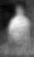
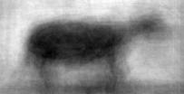
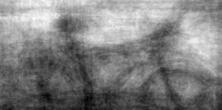
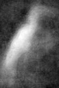
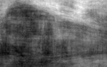
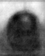
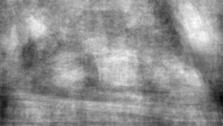
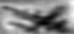
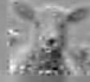
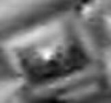
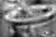
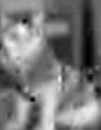
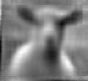
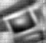
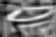
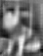
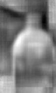
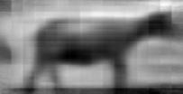
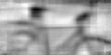
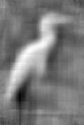
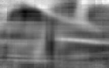
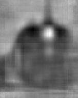
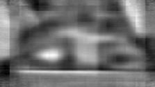
We show our inversions in Figure 9 for a few object categories. Exemplar LDA and ridge regression tend to produce blurred visualizations. Direct optimization recovers high frequency details at the expense of extra noise. Paired dictionary learning tends to produce the best visualization for HOG descriptors. By learning a dictionary over the visual world and the correlation between HOG and natural images, paired dictionary learning recovered high frequencies without introducing significant noise.

Figure 10: We show results where our paired dictionary algorithm is trained to recover RGB images instead of only grayscale images. The right shows the original image and the left shows the inverse.

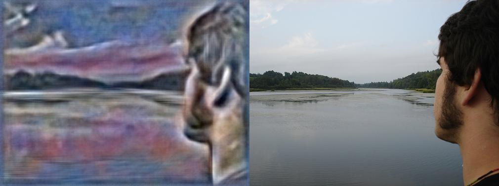
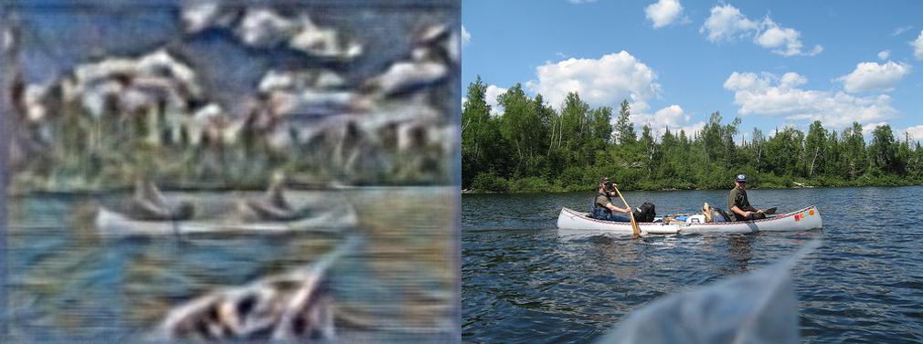
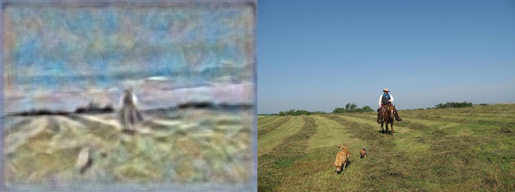
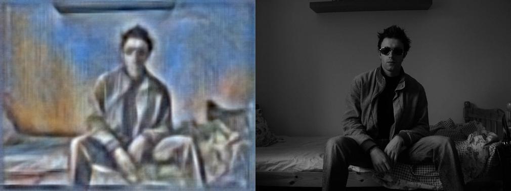
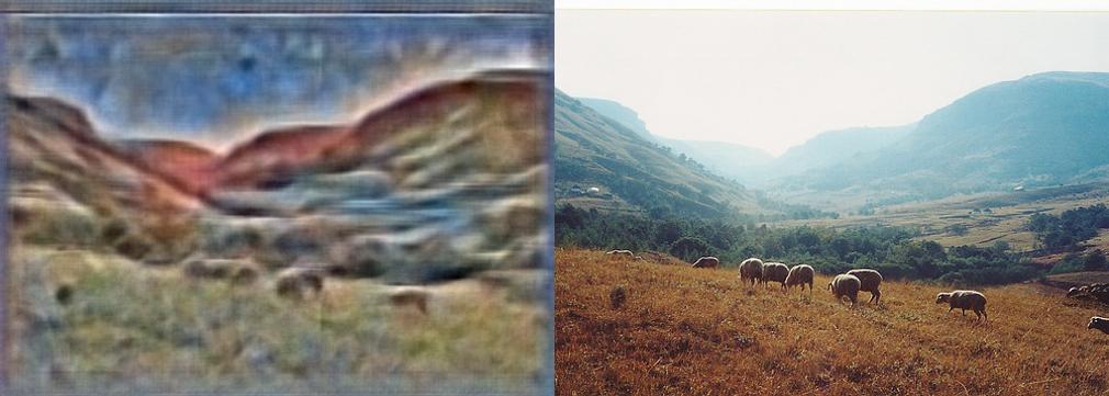
Although HOG does not explicitly encode color, we found that the paired dictionary is able to recover color from HOG descriptors. Figure 10 shows the result of training a paired dictionary to estimate RGB images instead of grayscale images. While the paired dictionary assigns arbitrary colors to man-made objects and indoor scenes, it frequently colors natural objects correctly, such as grass or the sky, likely because those categories are strongly correlated to HOG descriptors. We focus on grayscale visualizations in this paper because we found those to be more intuitive for humans to understand.

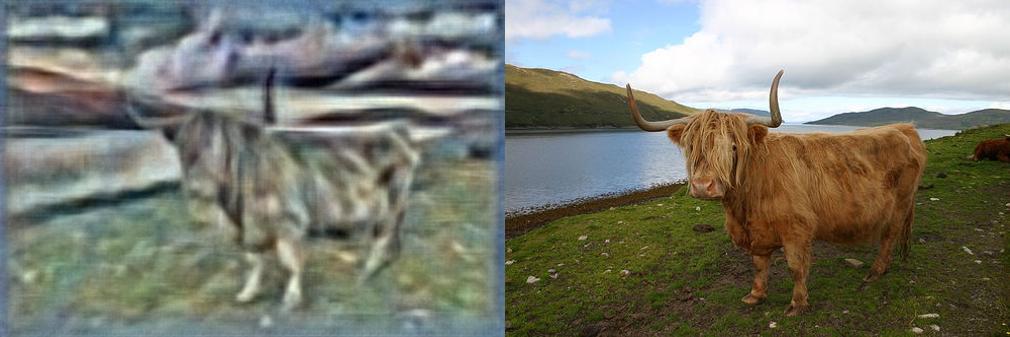
We also explored whether our visualization algorithm could invert other features besides HOG, such as deep features. Figure 14 shows how our algorithm can recover some details of the original image given only activations from the last convolutional layer of Krizhevsky et al (2012). Although the visualizations are blurry, they do capture some important visual aspects of the original images such as shapes and colors. This suggests that our visualization algorithm may be general to the type of feature.

(a) Original

(b) PairDict (seconds)

(c) Greedy (days)

Figure 11: Although our algorithms are good at inverting HOG, they are not perfect, and struggle to reconstruct high frequency detail. See text for details.

(a) Original $x$

(b) $x^{\prime}=\phi^{-1}\left(\phi(x)\right)$

(c) $x^{\prime\prime}=\phi^{-1}\left(\phi(x^{\prime})\right)$

Figure 12: We recursively compute HOG and invert it with a paired dictionary. While there is some information loss, our visualizations still do a good job at accurately representing HOG features. $\phi(\cdot)$ is HOG, and $\phi^{-1}(\cdot)$ is the inverse.

(a) $40\times 40$

(b) $20\times 20$

(c) $10\times 10$

(d) $5\times 5$

Figure 13: Our inversion algorithms are sensitive to the HOG template size. We show how performance degrades as the template becomes smaller.

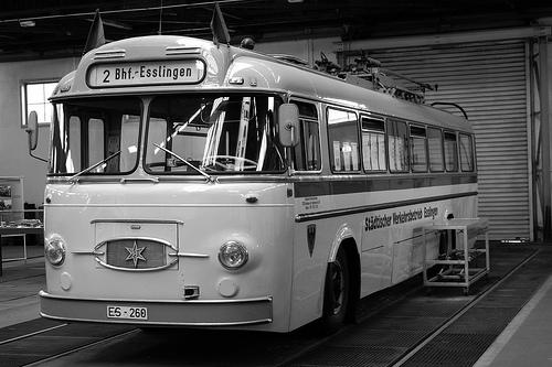
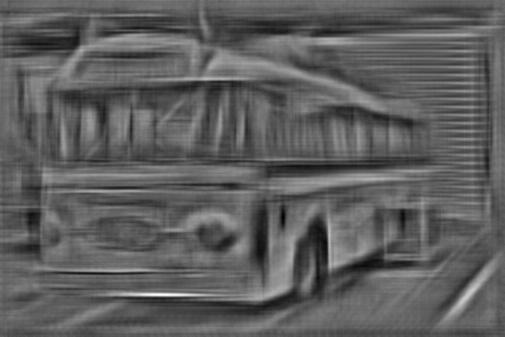
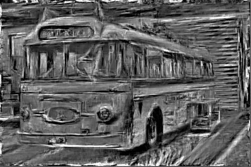
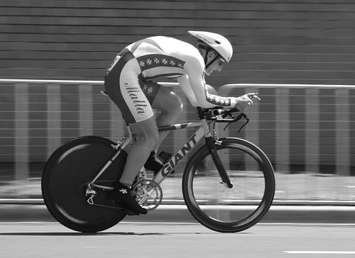
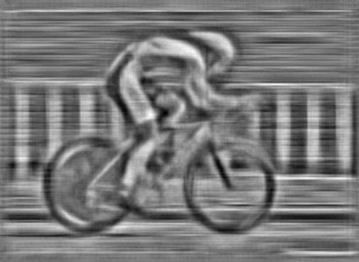
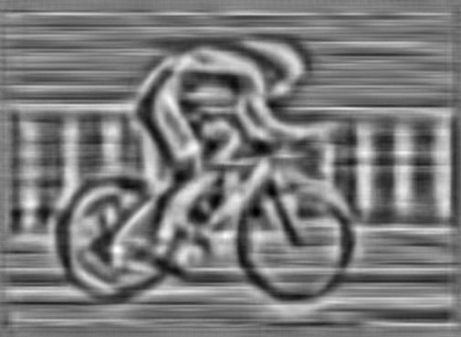
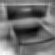
While our visualizations do a good job at representing HOG features, they have some limitations. Figure 11 compares our best visualization (paired dictionary) against a greedy algorithm that draws triangles of random rotation, scale, position, and intensity, and only accepts the triangle if it improves the reconstruction. If we allow the greedy algorithm to execute for an extremely long time (a few days), the visualization better shows higher frequency detail. This reveals that there exists a visualization better than paired dictionary learning, although it may not be tractable for large scale experiments. In a related experiment, Figure 12 recursively computes HOG on the inverse and inverts it again. This recursion shows that there is some loss between iterations, although it is minor and appears to discard high frequency details. Moreover, Figure 13 indicates that our inversions are sensitive to the dimensionality of the HOG template. Despite these limitations, our visualizations are, as we will now show, still perceptually intuitive for humans to understand.

5.2 Quantitative Results

We quantitatively evaluate our algorithms under two benchmarks. Firstly, we use an automatic inversion metric that measures how well our inversions reconstruct original images. Secondly, we conducted a large visualization challenge with human subjects on Amazon Mechanical Turk (MTurk), which is designed to determine how well people can infer high level semantics from our visualizations.

Pixel Level Reconstruction: We consider the inversion performance of our algorithm: given a HOG feature $y$, how well does our inverse $\phi^{-1}(y)$ reconstruct the original pixels $x$ for each algorithm? Since HOG is invariant up to a constant shift and scale, we score each inversion against the original image with normalized cross correlation. Our results are shown in Table 1. Overall, exemplar LDA does the best at pixel level reconstruction.

Semantic Reconstruction: While the inversion benchmark evaluates how well the inversions reconstruct the original image, it does not capture the high level content of the inverse: is the inverse of a sheep still a sheep? To evaluate this, we conducted a study on MTurk. We sampled 2,000 windows corresponding to objects in PASCAL VOC 2011. We then showed participants an inversion from one of our algorithms and asked participants to classify it into one of the 20 categories. Each window was shown to three different users. Users were required to pass a training course and qualification exam before participating in order to guarantee users understood the task. Users could optionally select that they were not confident in their answer. We also compared our algorithms against the standard black-and-white HOG glyph popularized by (Dalal and Triggs, 2005).

Figure 14: We show visualizations from our method to invert features from deep convolutional networks. Although the visualizations are blurry, they capture some key aspects of the original images, such as shapes and colors. Our visualizations are inverting the last convolutional layer of Krizhevsky et al (2012).

Category	ELDA	Ridge	Direct	PairDict
aeroplane	0.634	0.633	0.596	0.609
bicycle	0.452	0.577	0.513	0.561
bird	0.680	0.650	0.618	0.638
boat	0.697	0.678	0.631	0.629
bottle	0.697	0.683	0.660	0.671
bus	0.627	0.632	0.587	0.585
car	0.668	0.677	0.652	0.639
cat	0.749	0.712	0.687	0.705
chair	0.660	0.621	0.604	0.617
cow	0.720	0.663	0.632	0.650
table	0.656	0.617	0.582	0.614
dog	0.717	0.676	0.638	0.667
horse	0.686	0.633	0.586	0.635
motorbike	0.573	0.617	0.549	0.592
person	0.696	0.667	0.646	0.646
pottedplant	0.674	0.679	0.629	0.649
sheep	0.743	0.731	0.692	0.695
sofa	0.691	0.657	0.633	0.657
train	0.697	0.684	0.634	0.645
tvmonitor	0.711	0.640	0.638	0.629
Mean	0.671	0.656	0.620	0.637

Table 1: We evaluate the performance of our inversion algorithm by comparing the inverse to the ground truth image using the mean normalized cross correlation. Higher is better; a score of 1 is perfect.

Category	ELDA	Ridge	Direct	PairDict	Glyph	Expert
aeroplane	0.433	0.391	0.568	0.645	0.297	0.333
bicycle	0.327	0.127	0.362	0.307	0.405	0.438
bird	0.364	0.263	0.378	0.372	0.193	0.059
boat	0.292	0.182	0.255	0.329	0.119	0.352
bottle	0.269	0.282	0.283	0.446	0.312	0.222
bus	0.473	0.395	0.541	0.549	0.122	0.118
car	0.397	0.457	0.617	0.585	0.359	0.389
cat	0.219	0.178	0.381	0.199	0.139	0.286
chair	0.099	0.239	0.223	0.386	0.119	0.167
cow	0.133	0.103	0.230	0.197	0.072	0.214
table	0.152	0.064	0.162	0.237	0.071	0.125
dog	0.222	0.316	0.351	0.343	0.107	0.150
horse	0.260	0.290	0.354	0.446	0.144	0.150
motorbike	0.221	0.232	0.396	0.224	0.298	0.350
person	0.458	0.546	0.502	0.676	0.301	0.375
pottedplant	0.112	0.109	0.203	0.091	0.080	0.136
sheep	0.227	0.194	0.368	0.253	0.041	0.000
sofa	0.138	0.100	0.162	0.293	0.104	0.000
train	0.311	0.244	0.316	0.404	0.173	0.133
tvmonitor	0.537	0.439	0.449	0.682	0.354	0.666
Mean	0.282	0.258	0.355	0.383	0.191	0.233

Table 2: We evaluate visualization performance across twenty PASCAL VOC categories by asking MTurk participants to classify our inversions. Numbers are percent classified correctly; higher is better. Chance is $0.05$. Glyph refers to the standard black-and-white HOG diagram popularized by (Dalal and Triggs, 2005). Paired dictionary learning provides the best visualizations for humans. Expert refers to MIT PhD students in computer vision performing the same visualization challenge with HOG glyphs.

Our results in Table 2 show that paired dictionary learning and direct optimization provide the best visualization of HOG descriptors for humans. Ridge regression and exemplar LDA perform better than the glyph, but they suffer from blurred inversions. Human performance on the HOG glyph is generally poor, and participants were even the slowest at completing that study. Interestingly, the glyph does the best job at visualizing bicycles, likely due to their unique circular gradients. Our results overall suggest that visualizing HOG with the glyph is misleading, and richer visualizations from our paired dictionary are useful for interpreting HOG features.

Our experiments suggest that humans can predict the performance of object detectors by only looking at HOG visualizations. Human accuracy on inversions and state-of-the-art object detection AP scores from (Felzenszwalb et al, 2010a) are correlated with a Spearman’s rank correlation coefficient of 0.77.

We also asked computer vision PhD students at MIT to classify HOG glyphs in order to compare MTurk participants with experts in HOG. Our results are summarized in the last column of Table 2. HOG experts performed slightly better than non-experts on the glyph challenge, but experts on glyphs did not beat non-experts on other visualizations. This result suggests that our algorithms produce more intuitive visualizations even for object detection researchers.

6 Evaluation of Multiple Inversions

Since features are many-to-one functions, our visualization algorithms should be able to recover multiple inversions for a feature descriptor. We look at the multiple inversions from deep network features because these features appear to be robust to several invariances.

To conduct our experiments with multiple inversions, we inverted features from the AlexNet convolutional neural network (Krizhevsky et al, 2012) trained on ImageNet (Deng et al, 2009; Russakovsky et al, 2014). We use the publicly available Caffe software package (Jia, 2013) to extract features. We use features from the last convolutional layer (pool5), which has been shown to have strong performance on recognition tasks (Girshick et al, 2013). We trained the dictionaries $U$ and $V$ using random windows from the PASCAL VOC 2007 training set (Everingham et al, 2010). We tested on two thousand random windows corresponding to objects in the held-out PASCAL VOC 2007 validation set.

(a) Affinity = Color

(b) Affinity = Edge

(c) Nudged Dict

(d) Subset Dict

Figure 15: We show the first three inversions for a few patches from our testing set. Notice how the color (a) and edge (b) variants of our method tend to produce different inversions. The baselines tend to either similar in image space (c) or do not match well in feature space (d). Best viewed on screen.

Figure 16: The edge affinity can often result in subtle differences. Above, we show a difference matrix between the first three inversions that highlights differences between all pairs of a few inversions from one CNN feature. The margins show the inversions, and the inner black squares show the absolute difference. White means larger difference. Notice that our algorithm is able to recover inversions with shifts of gradients.

6.1 Qualitative Results

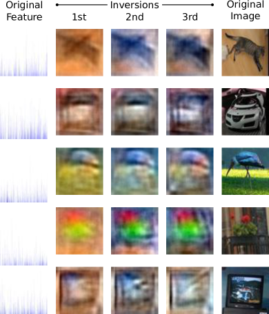
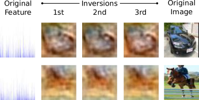
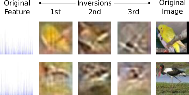
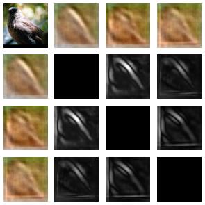
We first look at a few qualitative results for our multiple feature inversions. Figure 15 shows a few examples for both our method (top rows) and the baselines (bottom rows). The 1st column shows the result of a paired dictionary on CNN features, while the 2nd and 3rd show the additional inversions that our method finds. While the results are blurred, they do tend to resemble the original image in rough shape and color.

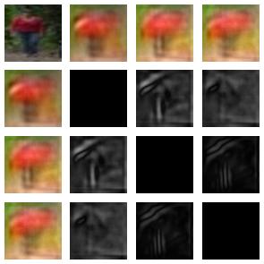
The color affinity in Figure 15a is often able to produce inversions that vary slightly in color. Notice how the cat and the floor are changing slightly in hue, and the grass the bird is standing on is varying slightly. The edge affinity in Figure 15b can occasionally generate inversions with different edges, although the differences can be subtle. To better show the differences with the edge affinity, we visualize a difference matrix in Figure 16. Notice how the edges of the bird and person shift between each inversion.

Figure 17: The block-wise histograms of HOG allow for gradients in the image to shift up to their bin size without affecting the feature descriptor. By using our visualization algorithm with the edge affinity matrix, we can recover multiple HOG inversions that differ by edges subtly shifting. Above, we show a difference matrix between the first three inversions for a downsampled image of a man shown in the top left corner. Notice the vertical gradient in the background shifts between the inversions, and the man’s head move slightly.

The baselines tend to either produce nearly identical inversions or inversions that do not match well in feature space. Nudged dictionaries in Figure 15c frequently retrieves inversions that look nearly identical. Subset dictionaries in Figure 15d recovers different inversions, but the inversions do not match in feature space, likely because this baseline operates over a subset of the basis elements.

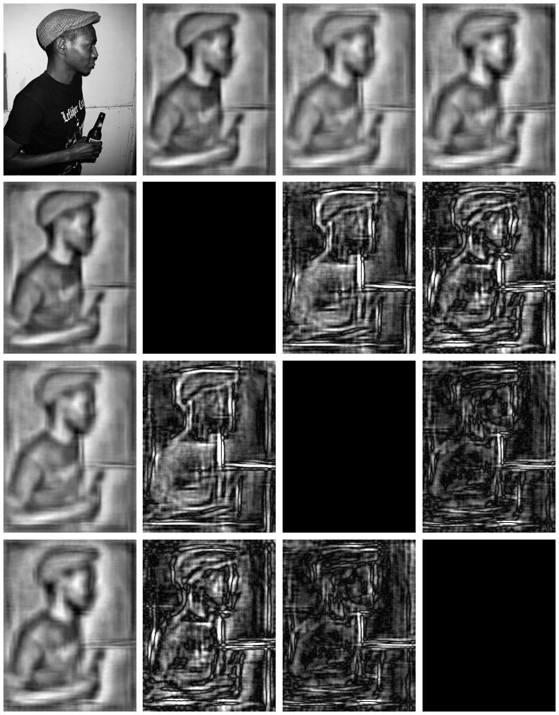
Although HOG is not as invariant to visual transformations as deep features, we can still recover multiple inversions from a HOG descriptor. The block-wise histograms of HOG allow for gradients in the image to shift up to their bin size without affecting the feature descriptor. Figure 17 shows multiple inversions from a HOG descriptor of a man where the person shifts slightly between each inversion.

6.2 Quantitative Results

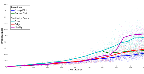
We wish to quantify how well our inversions trade off matching in feature space versus having diversity in image space. To evaluate this, we calculated Euclidean distance between the features of the first and second inversions from each method, $||\phi(x_{1})-\phi(x_{2})||_{2}$, and compared it to the Euclidean distance of the inversions in Lab image space, $||L(x_{1})-L(x_{2})||_{2}$ where $L(\cdot)$ is the Lab colorspace transformation. We consider one inversion algorithm to be better than another method if, for the same distance in feature space, the image distance is larger.

We show a scatter plot of this metric in Figure 18 for our method with different similarity costs. The thick lines show the median image distance for a given feature distance. The overall trend suggests that our method produces more diverse images for the same distance in feature space. Setting the affinity matrix $A$ to perform color averaging produces the most image variation for CNN features in order to keep the feature space accuracy small. The baselines in general do not perform as well, and baseline with subset dictionaries struggles to even match in feature space, causing the green line to abruptly start in the middle of the plot. The edge affinity produces inversions that tend to be more diverse than baselines, although this effect is best seen qualitatively in the next section.

We consider a second evaluation metric designed to determine how well our inversions match the original features. Since distances in a feature space are unscaled, they can be difficult to interpret, so we use a normalized metric. We calculate the ratio of distances that the inversions make to the original feature: $r=\frac{||\phi(x_{2})-f||_{2}}{||\phi(x_{1})-f||_{2}}$ where $f$ is the original feature and $x_{1}$ and $x_{2}$ are the first and second inversions. A value of $r=1$ implies the second inversion is just as close to $f$ as the first. We then compare the ratio $r$ to the Lab distance in image space.

Figure 18: We evaluate the performance of our multiple inversion algorithm. The horizontal axis is the Euclidean distance between the first and second inversion in CNN space and the vertical axis is the distance of the same inversions in Lab colorspace. This plot suggests that incorporating diversity costs into the inversion are able to produce more diverse multiple visualizations for the same reconstruction error. Thick lines show the median image distance for a given feature distance.

(a) Color

(b) Identity

(c) Edge

(d) Nudged Dict

(e) Subset Dict

Figure 19: We show density maps that visualize image distance versus the ratio distances in feature space: $r=\frac{||\phi(x_{2})-f||_{2}}{||\phi(x_{1})-f||_{2}}$. A value of $r=1$ means that the two inversions are the same distance from the original feature. Black means most dense and white is zero density. Our results suggest that our method with the affinity matrix set to color averaging produces more diverse visualizations for the same $r$ value.

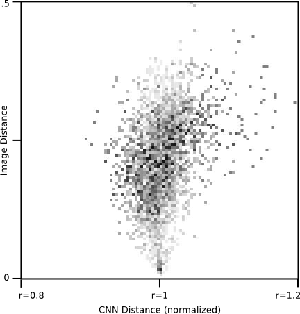
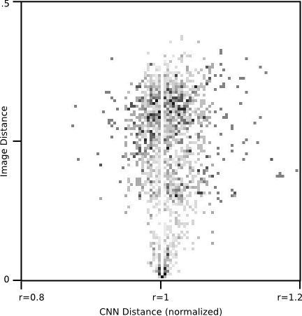
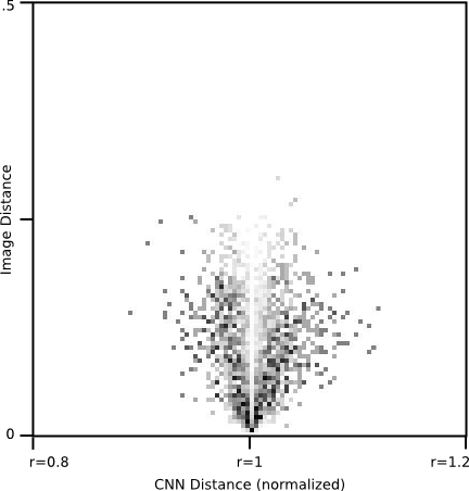
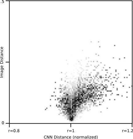
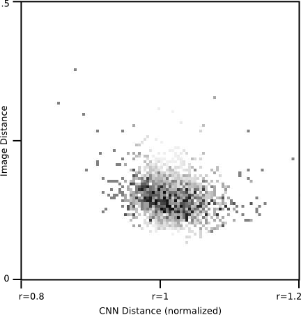
We show results for our second metric in Figure 19 as a density map comparing image distance and the ratio of distances in feature space. Black is a higher density and implies that the method produces inversions in that region more frequently. This experiment shows that for the same ratio $r$, our approach tends to produce more diverse inversions when affinity is set to color averaging. Baselines frequently performed poorly, and struggled to generate diverse images that are close in feature space.

7 Understanding Object Detectors

While the goal of this paper is to visualize object detection features, in this section we will use our visualizations to inspect the behavior of object detection systems. Due to our budget for experiments, we focus on HOG features.

7.1 HOGgles

Our visualizations reveal that the world that features see is slightly different from the world that the human eye perceives. Figure 20a shows a normal photograph of a man standing in a dark room, but Figure 20b shows how HOG features see the same man. Since HOG is invariant to illumination changes and amplifies gradients, the background of the scene, normally invisible to the human eye, materializes in our visualization.

In order to understand how this clutter affects object detection, we visualized the features of some of the top false alarms from the Felzenszwalb et al. object detection system (Felzenszwalb et al, 2010b) when applied to the PASCAL VOC 2007 test set. Figure 3 shows our visualizations of the features of the top false alarms. Notice how the false alarms look very similar to true positives. While there are many different types of detector errors, this result suggests that these particular failures are due to limitations of HOG, and consequently, even if we develop better learning algorithms or use larger datasets, these will false alarms will likely persist.

Figure 23 shows the corresponding RGB image patches for the false positives discussed above. Notice how when we view these detections in image space, all of the false alarms are difficult to explain. Why do chair detectors fire on buses, or people detectors on cherries? By visualizing the detections in feature space, we discovered that the learning algorithm made reasonable failures since the features are deceptively similar to true positives.

7.2 Human+HOG Detectors

Although HOG features are designed for machines, how well do humans see in HOG space? If we could quantify human vision on the HOG feature space, we could get insights into the performance of HOG with a perfect learning algorithm (people). Inspired by Parikh and Zitnick’s methodology (Parikh and Zitnick, 2011, 2010), we conducted a large human study where we had Amazon Mechanical Turk participants act as sliding window HOG based object detectors.

We built an online interface for humans to look at HOG visualizations of window patches at the same resolution as DPM. We instructed participants to either classify a HOG visualization as a positive example or a negative example for a category. By averaging over multiple people (we used 25 people per window), we obtain a real value score for a HOG patch. To build our dataset, we sampled top detections from DPM on the PASCAL VOC 2007 dataset for a few categories. Our dataset consisted of around $5,000$ windows per category and around $20\%$ were true positives.

(a) Human Vision

(b) HOG Vision

Figure 20: Feature inversion reveals the world that object detectors see. The left shows a man standing in a dark room. If we compute HOG on this image and invert it, the previously dark scene behind the man emerges. Notice the wall structure, the lamp post, and the chair in the bottom right hand corner.

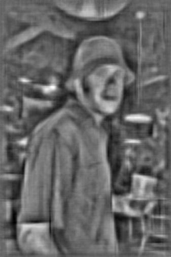
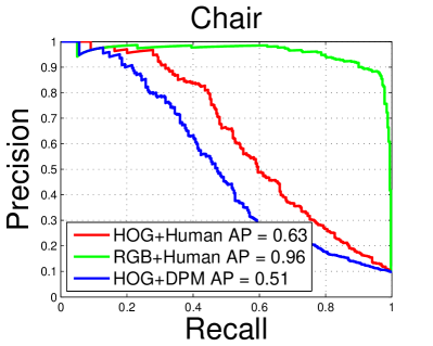
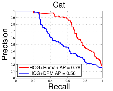
Figure 21 shows precision recall curves for the Human + HOG based object detector. In most cases, human subjects classifying HOG visualizations were able to rank sliding windows with either the same accuracy or better than DPM. Humans tied DPM for recognizing cars, suggesting that performance may be saturated for car detection on HOG. Humans were slightly superior to DPM for chairs, although performance might be nearing saturation soon. There appears to be the most potential for improvement for detecting cats with HOG. Subjects performed slightly worst than DPM for detecting people, but we believe this is the case because humans tend to be good at fabricating people in abstract drawings.

We then repeated the same experiment as above on chairs except we instructed users to classify the original RGB patch instead of the HOG visualization. As expected, humans have near perfect accuracy at detecting chairs with RGB sliding windows. The performance gap between the Human+HOG detector and Human+RGB detector demonstrates the amount of information that HOG features discard.

Figure 21: By instructing multiple human subjects to classify the visualizations, we show performance results with an ideal learning algorithm (i.e., humans) on the HOG feature space. Please see text for details.

Figure 22: We visualize a few deformable parts models trained with (Felzenszwalb et al, 2010b). Notice the structure that emerges with our visualization. First row: car, person, bottle, bicycle, motorbike, potted plant. Second row: train, bus, horse, television, chair. For the right most visualizations, we also included the HOG glyph. Our visualizations tend to reveal more detail than the glyph.

Figure 23: We show the original RGB patches that correspond to the visualizations from Figure 3. We print the original patches on a separate page to highlight how the inverses of false positives look like true positives. We recommend comparing this figure side-by-side with Figure 3.

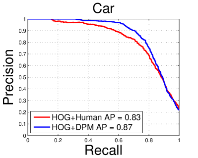
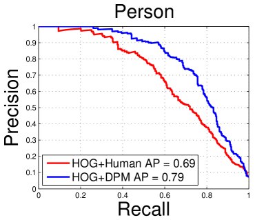
Our experiments suggest that there is still some performance left to be squeezed out of HOG. However, DPM is likely operating very close to the performance limit of HOG. Since humans are the ideal learning agent and they still had trouble detecting objects in HOG space, HOG may be too lossy of a descriptor for high performance object detection. If we wish to significantly advance the state-of-the-art in recognition, we suspect focusing effort on building better features that capture finer details as well as higher level information will lead to substantial performance improvements in object detection. Indeed, recent advances in object recognition have been driven by learning with richer features (Girshick et al, 2013).

7.3 Model Visualization

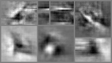
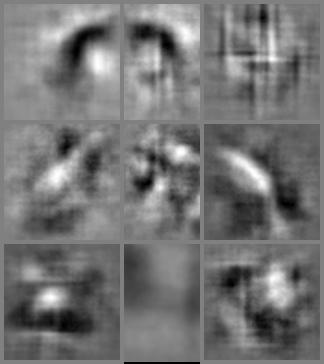
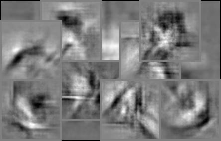
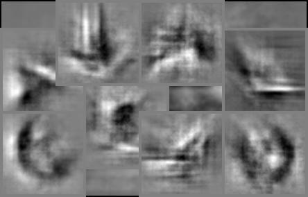
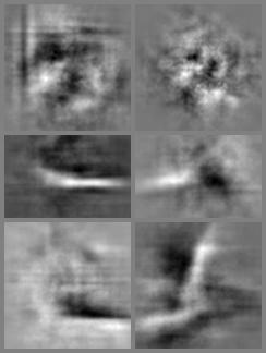
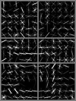
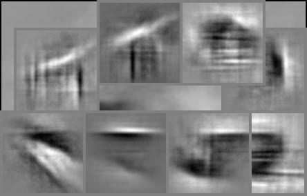
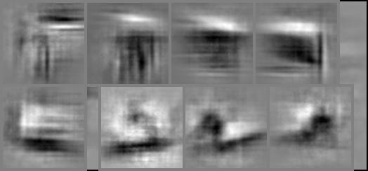
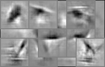
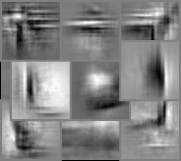
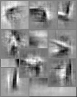
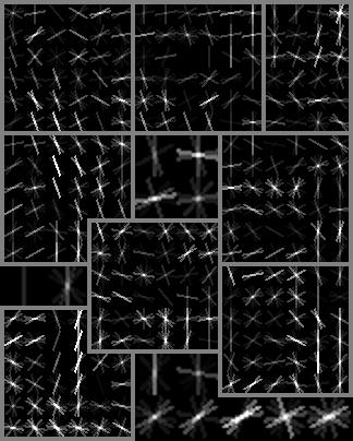
We found our algorithms are also useful for visualizing the learned models of an object detector. Figure 22 visualizes the root templates and the parts from (Felzenszwalb et al, 2010b) by inverting the positive components of the learned weights. These visualizations provide hints on which gradients the learning found discriminative. Notice the detailed structure that emerges from our visualization that is not apparent in the HOG glyph. Often, one can recognize the category of the detector by only looking at the visualizations.

8 Conclusion

We believe visualizations can be a powerful tool for understanding object detection systems and advancing research in computer vision. To this end, this paper presented and evaluated several algorithms to visualize object detection features. We hope more intuitive visualizations will prove useful for the community.

Acknowledgments: We thank the CSAIL Vision Group for many important discussions. Funding was provided by a NSF GRFP to CV, a Facebook fellowship to AK, and a Google research award, ONR MURI N000141010933 and NSF Career Award No. 0747120 to AT.

References

- Alahi et al (2012) Alahi A, Ortiz R, Vandergheynst P (2012) Freak: Fast retina keypoint. In: CVPR
- Biggio et al (2012) Biggio B, Nelson B, Laskov P (2012) Poisoning attacks against support vector machines. ICML
- Bruckner (2014) Bruckner D (2014) Ml-o-scope: a diagnostic visualization system for deep machine learning pipelines
- Calonder et al (2010) Calonder M, Lepetit V, Strecha C, Fua P (2010) Brief: Binary robust independent elementary features. ECCV
- Chen and Grauman (2014) Chen CY, Grauman K (2014) Inferring unseen views of people
- Dalal and Triggs (2005) Dalal N, Triggs B (2005) Histograms of oriented gradients for human detection. In: CVPR
- d’Angelo et al (2012) d’Angelo E, Alahi A, Vandergheynst P (2012) Beyond bits: Reconstructing images from local binary descriptors. ICPR
- Deng et al (2009) Deng J, Dong W, Socher R, Li LJ, Li K, Fei-Fei L (2009) Imagenet: A large-scale hierarchical image database. In: CVPR
- Divvala et al (2012) Divvala S, Efros A, Hebert M (2012) How important are deformable parts in the deformable parts model? Technical Report
- Everingham et al (2010) Everingham M, Van Gool L, Williams CKI, Winn J, Zisserman A (2010) The pascal visual object classes challenge. IJCV
- Felzenszwalb et al (2010a) Felzenszwalb P, Girshick R, McAllester D (2010a) Cascade object detection with deformable part models. In: CVPR
- Felzenszwalb et al (2010b) Felzenszwalb P, Girshick R, McAllester D, Ramanan D (2010b) Object detection with discriminatively trained part-based models. PAMI
- Girshick et al (2013) Girshick R, Donahue J, Darrell T, Malik J (2013) Rich feature hierarchies for accurate object detection and semantic segmentation. arXiv preprint arXiv:13112524
- Hariharan et al (2012) Hariharan B, Malik J, Ramanan D (2012) Discriminative decorrelation for clustering and classification. ECCV
- Hoiem et al (2012) Hoiem D, Chodpathumwan Y, Dai Q (2012) Diagnosing error in object detectors. ECCV
- Huang and Wang (2013) Huang DA, Wang YCF (2013) Coupled dictionary and feature space learning with applications to cross-domain image synthesis and recognition
- Jain (1989) Jain AK (1989) Fundamentals of digital image processing. Prentice-Hall, Inc.
- Jia (2013) Jia Y (2013) Caffe: An open source convolutional architecture for fast feature embedding
- Kato and Harada (2014) Kato H, Harada T (2014) Image reconstruction from bag-of-visual-words. In: CVPR
- Krizhevsky et al (2012) Krizhevsky A, Sutskever I, Hinton GE (2012) Imagenet classification with deep convolutional neural networks. In: NIPS
- Lenc and Vedaldi (2014) Lenc K, Vedaldi A (2014) Understanding image representations by measuring their equivariance and equivalence
- Liu and Wang (2012) Liu L, Wang L (2012) What has my classifier learned? visualizing the classification rules of bag-of-feature model by support region detection. In: CVPR
- Lowe (1999) Lowe D (1999) Object recognition from local scale-invariant features. In: ICCV
- Mahendran and Vedaldi (2014) Mahendran A, Vedaldi A (2014) Understanding Deep Image Representations by Inverting Them
- Mairal et al (2009) Mairal J, Bach F, Ponce J, Sapiro G (2009) Online dictionary learning for sparse coding. In: ICML
- Malisiewicz et al (2011) Malisiewicz T, Gupta A, Efros A (2011) Ensemble of exemplar-svms for object detection and beyond. In: ICCV
- Nishimoto et al (2011) Nishimoto S, Vu A, Naselaris T, Benjamini Y, Yu B, Gallant J (2011) Reconstructing visual experiences from brain activity evoked by natural movies. Current Biology
- Oliva and Torralba (2001) Oliva A, Torralba A (2001) Modeling the shape of the scene: A holistic representation of the spatial envelope. IJCV
- Parikh and Zitnick (2011) Parikh D, Zitnick C (2011) Human-debugging of machines. In: NIPS WCSSWC
- Parikh and Zitnick (2010) Parikh D, Zitnick CL (2010) The role of features, algorithms and data in visual recognition. In: CVPR
- Russakovsky et al (2014) Russakovsky O, Deng J, Su H, Krause J, Satheesh S, Ma S, Huang Z, Karpathy A, Khosla A, Bernstein M, et al (2014) Imagenet large scale visual recognition challenge. arXiv preprint arXiv:14090575
- Sadeghi and Forsyth (2013) Sadeghi MA, Forsyth D (2013) Fast template evaluation with vector quantization. In: NIPS
- Simonyan et al (2013) Simonyan K, Vedaldi A, Zisserman A (2013) Deep inside convolutional networks: Visualising image classification models and saliency maps. arXiv preprint
- Tatu et al (2011) Tatu A, Lauze F, Nielsen M, Kimia B (2011) Exploring the representation capabilities of hog descriptors. In: ICCV WIT
- Vondrick et al (2013) Vondrick C, Khosla A, Malisiewicz T, Torralba A (2013) Hoggles: Visualizing object detection features. In: ICCV
- Wang et al (2012) Wang S, Zhang L, Liang Y, Pan Q (2012) Semi-coupled dictionary learning with applications to image super-resolution and photo-sketch synthesis. In: CVPR
- Weinzaepfel et al (2011) Weinzaepfel P, Jégou H, Pérez P (2011) Reconstructing an image from its local descriptors. In: CVPR
- Yang et al (2010) Yang J, Wright J, Huang T, Ma Y (2010) Image super-resolution via sparse representation. Transactions on Image Processing
- Zeiler and Fergus (2013) Zeiler MD, Fergus R (2013) Visualizing and understanding convolutional neural networks. arXiv preprint arXiv:13112901
- Zhang et al (2014) Zhang L, Dibeklioglu H, van der Maaten L (2014) Speeding up tracking by ignoring features. CVPR
- Zhu et al (2012) Zhu X, Vondrick C, Ramanan D, Fowlkes C (2012) Do we need more training data or better models for object detection? BMVC
- Zou and Hastie (2005) Zou H, Hastie T (2005) Regularization and variable selection via the elastic net. Journal of the Royal Statistical Society: Series B (Statistical Methodology)