Multibin correlations in a superposition approach to relativistic heavy-ion collisions

Abstract

Analysis of correlation of multiplicities between various rapidity bins is carried out in the framework of a superposition approach consisting of three phases of the ultra-relativistic nuclear collision: early partonic phase, intermediate collective evolution, and statistical hadronization. Simple relations between the moments of produced hadrons and the moments of the sources produced in the initial partonic phase are presented. They involve only a few effective parameters describing the microscopic dynamics of the system. We illustrate the practicality of the approach with the Glauber model simulations. Our study bears direct relevance for the interpretation of the upcoming results for the multibin multiplicity correlations from the LHC, which will help in an assessment of the correlation features of the state formed in the earliest stage of the reaction.

I Introduction

Long-range rapidity correlations between multiplicities of produced hadrons have been under active consideration since the early experiments with $pp$ and $p\bar{p}$ collisions Uhlig:1977dc ; Alpgard:1983xp ; Ansorge:1988fg ; Alexopoulos:1995ft , followed with heavy-ion data in the RHIC era Abelev:2009ag ; Tarnowsky:2010qp ; ATLAS:2012as . Numerous theoretical investigations followed, in particular Capella:1978rg ; Amelin:1994mf ; Braun:2000cc ; Braun:2003fn ; Brogueira:2007ub ; Armesto:2007ia ; Armesto:2006bv ; Vechernin:2007zza ; Braun:2007rf ; Konchakovski:2008cf ; Bzdak:2009dr ; Lappi:2009vb ; Bozek:2010vz ; deDeus:2010id ; Bzdak:2011nb ; Bzdak:2012tp ; Vechernin:2012bz ; Bialas:2013xea ; De:2013bta ; Ma:2014pva . The interest is driven by the expectation that such correlations may provide understanding of the elementary space-time dynamics in the earliest (partonic) stages of the reaction. An extension of the conventional forward-backward analysis based on multibin correlations in rapidity and applying factorial moments has been developed in Bialas:2011xk ; Bialas:2011vj .

We recall that according to the interpretation of the STAR Collaboration data of Ref. Tarnowsky:2010qp ; ATLAS:2012as , made in Lappi:2009vb ; Bzdak:2011nb , we are quite far from understanding theoretically in a complete way the forward-backward correlations in heavy-ion collisions, in particular their centrality dependence. With the analyses from the Large Hadron Collider (LHC) expected to be released in the near future, it is important to prepare theoretical ground for the interpretation of the data, which is one of the goals of our work.

In this paper, which extends the analysis of Ref. Olszewski:2013qwa to the case of three bins (forward, central, and backward), we analyze the pseudorapidity correlations in a superposition approach. In this framework, to describe the statistical aspects of relativistic heavy-ion dynamics we use a common picture involving three separate stages: 1) early generation of initial partonic densities (sources), 2) collective (hydrodynamic or transport) evolution, and 3) statistical hadronization. A crucial assumption for the method is that the emission from a source is independent from other sources and universal, i.e., occurs from the same statistical distribution independently of the rapidity or the centrality class of the collision. This leads to very simple formulas for the statistical measures, relating the moments of the initial sources to the moments of the distribution of the produced hadrons, in particular the multibin correlation coefficients. Parameters present in these relations depend on the features of the overlaid statistical distributions and properties of hydrodynamics, and have simple interpretation.

We use the derived relations to obtain predictions for multiplicities, variances, and multibin correlations of the produced hadrons. To model the initial phase, we use the Glauber framework based on wounded nucleons Bialas:1976ed ; Bialas:2008zza ; Broniowski:2007ft amended with binary collisions Kharzeev:2000ph ; SchaffnerBielich:2001qj ; Back:2001xy . The predictions are made for the Pb+Pb collisions at $\sqrt{s_{NN}}=2.76\textrm{~{}TeV}$, as the corresponding analyses from the LHC are expected to be published in the near future.

We note that simulations of the forward-backward multiplicity correlations for the Au+Au collisions at the highest RHIC energies were carried out by Konchakovski et al. Konchakovski:2008cf in the framework of the wounded-nucleon model with overlaid Poisson distribution and in the Hadron-String-Dynamics transport approach Ehehalt:1996uq . That work carefully discusses the influence of centrality selection on the correlation measures used in the experiment, pointing out to effects stemming just from the fact that the centrality classes are wide. Our results from the Glauber model comply to these general findings.

Our paper is organized as follows. In Sec. II we review the three-stage approach, consisting of the early production, the hydrodynamic evolution, and the final freeze-out. We derive the relations between the multibin moments of the sources produced in the early phase and of the multibin moments of final hadrons. Some general predictions of the approach are given in Sec. III. In Sec. IV we discuss the technically important issues related to the choice of the centrality bins. For the considered statistical measures, scaling laws with the width of the centrality bin are derived. Section V presents our results of the Glauber simulations for the initial phase. We show here the practicality of our method in the application to the future experimental data, which will serve to verify the model of the initial phase.

II Three stage approach

Figure 1: (color online) Time evolution of the created system, visualizing the subsequent stages of particle production. B, C, and F indicate the backward, central, and forward bins, respectively, extending along the spatial rapidity or pseudorapidity direction.

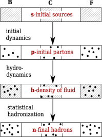
In Ref. Olszewski:2013qwa we have considered a three-stage approach, based on superposition, that describes certain features of production of particles in relativistic heavy ion collisions and their correlations, focusing entirely on statistical aspects. In this framework, the complicated dynamical evolution of the system is represented with the following separate stages:

1. Initial phase, which may be modeled with the Glauber approach Czyz:1969jg ; Bialas:1976ed ; Bialas:2008zza ; Kharzeev:2000ph ; Back:2001xy ; Broniowski:2007ft , color glass condensate Kovner:1995ja ; Iancu:2000hn ; Lappi:2010cp ; Lappi:2011zz , string formation Amelin:1994mf ; Brogueira:2006yk , etc. As the result of this early dynamics, some initial space-time distribution of entropy or energy-density is generated. We assume that first the initial sources are formed (see Sec. II.1), denoted with $s$, which then produce the distribution of initial partons, $p$ (see top of Fig. 1). The extent of correlation between the source densities in spatial rapidity bins $B$, $C$, or $F$ depends on the early dynamics.

2. Hydrodynamic evolution (for reviews see, e.g., Heinz:2013th ; Gale:2013da and references therein) or transport Lin:2004en evolves the initial density of partons $p$ into expanding hydrodynamic fluid density $h$ (third row in Fig. 1). In our considerations it is only important that $h$ is (to a good approximation) proportional to $p$.

3. Freeze-out and the statistical hadronization mechanism (see, e.g., WFlorkowski:2010zz for a review), converting the hydrodynamic fluid into hadrons $n$, which are then subject to experimental observation in various pseudorapidity bins.

The above simple scheme summarizes most of the popular model approaches to particle production in relativistic heavy-ion collisions. Our treatment focuses on statistical aspects of each of the phases. While the underlining dynamical mechanisms are very complicated, it turns out that certain statistical features may be simply parametrized, and specific conclusions concerning particle correlations in rapidity may be, under mild assumptions, drawn in a model-independent way.

Figure 2: (color online) Initial source projected on the transverse plane (left) and the three dimensional picture of color flux-tubes extending along the spatial rapidity (right).

II.1 Sources

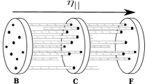
We use the concept of the initial sources, which yield the initial space-time entropy or energy density distribution. The precise definition depends on the model of the initial phase. In our work we use the Glauber model RGlauber:1959aa ; Czyz:1969jg ; Bialas:1976ed ; Miller:2007ri ; Broniowski:2007ft ; Bialas:2008zza , where the source is created in an individual NN collision, located in the transverse plane and extending along the spatial rapidity direction, $\eta_{\parallel}=\frac{1}{2}\log[(t+z)/(t-z)]$ (cf. Fig. 2). A particular model of the distribution in $\eta_{\parallel}$, coming from Ref. Bozek:2010bi and used here, is described in Appendix A. It is motivated with the success of Ref. Bialas:2004su in describing the deuteron-gold collisions Nouicer:2004ke , followed with the extension to NN collisions Gazdzicki:2005rr ; Bzdak:2009dr ; Bzdak:2009xq . We note that other descriptions of the early production could be used as well, for instance the Kharzeev-Levin-Nardi framework Kharzeev:2000ph ; Kharzeev:2002ei ; Drescher:2006pi .

In certain models, the sources may be interpreted as color flux-tubes, extending along some range in rapidity, as pictured in Fig. 2). It may happen that some flux-tubes are longer, extending through the whole region of interest from the $B$ to $F$ bins, while some may be shorter, as indicated in Fig. 2), making the correlations shorter-range. Clearly, such effects influence the multiplicity correlations between the bins, which is what ultimately we wish to investigate.

The dots in Fig. 2 indicate the sources in bin $A$, where $A=F,B,C$. Their corresponding numbers are denoted as $s_{A}$ throughout this paper.

II.2 Centrality definition

The number of sources in the central bin, $s_{C}$, is used to define the centrality classes of the collision in our simulations presented in Sec.  V. In the wounded nucleon model this prescription would correspond to using the number of wounded nucleons to determine centrality, as is frequently done in model studies. The definition based on wounded nucleons or participants of the projectile is appropriate for experiments which measure the projectile spectators in dedicated detectors (e.g, as in NA61). On the other hand, in experiments where the multiplicity of the event is used as the centrality selector, a closer measure would be the number of hadrons generated in the model, e.g., $n_{C}$. As pointed out in Ref. Konchakovski:2008cf , the definition of centrality may influence the results for the forward-backward correlations to some extent. We investigate this issue in Sec. V.3.

II.3 Initial dynamics

In the early stage of the reaction, the sources emit partons. We assume that each source produces partons independently of one another and, in addition, the production occurs independently in the $F$, $B$, and $C$ bins, as they are assumed to be well separated in the spatial rapidity $\eta_{\parallel}$. Thus, each source $i$ emits $\mu_{i}$ partons according to the same distribution,

$$\mathnormal{p_{A}=\sum_{i=1}^{s_{A}}\mu_{i},\quad A=B,F,C}.$$ (1)

It is then elementary to obtain the formulas for the above superposition model for moments corresponding to averages over events (here listed up to rank three):

$$\langle p_{A}\rangle = \langle\mu\rangle\langle s_{A}\rangle,$$

$$\langle\Delta p_{A}^{2}\rangle = {\rm var}(\mu)\langle s_{A}\rangle+\langle\mu\rangle^{2}\langle\Delta s_{A}^{2}\rangle,$$

$$\langle\Delta p_{A}\Delta p_{A^{\prime}}\rangle = \langle\mu\rangle^{2}\langle\Delta s_{A}\Delta s_{A^{\prime}}\rangle,$$

$$\langle\Delta p^{3}_{A}\rangle = \mu_{3}\!\left(\mu\right)\langle s_{A}\rangle+3{\rm var}(\mu)\langle\mu\rangle\langle\Delta s_{A}^{2}\rangle$$ (2)

$$+ \langle\mu\rangle^{3}\langle\Delta s_{A}^{3}\rangle,$$

$$\langle\Delta p_{A}\Delta p^{2}_{A^{\prime}}\rangle = {\rm var}(\mu)\langle\mu\rangle\langle\Delta s_{A}\Delta s_{A^{\prime}}\rangle$$

$$+ \langle\mu\rangle^{3}\langle\Delta s_{A}\Delta s^{2}_{A^{\prime}}\rangle,$$

$$\langle\Delta p_{F}\Delta p_{C}\Delta p_{B}\rangle = \langle\mu\rangle^{3}\langle\Delta s_{F}\Delta s_{C}\Delta s_{B}\rangle,$$

where $A,A^{\prime}=F$, $B$, or $C$, and $A\neq A^{\prime}$. In our notation $\Delta p_{A}^{n}=(p_{A}-\langle p_{A}\rangle)^{n}$, $n=1,2,3$, while $\langle\cdot\rangle$ denotes averaging over events. The symbol $\mu_{3}(x)$ stands for the third central moment of the distribution of $x$.

II.4 Hydrodynamics

The density of partons formed in the early phase, as described above, provides initial conditions for the equations of the hydrodynamic evolution of the fluid cell in the intermediate phase. This evolution, proceeding until freeze-out, is assumed to be deterministic (note, however, Refs. Kapusta:2011gt ; Kapusta:2012gm ), hence no extra fluctuations are introduced at this stage. As a result, the initial density of partons $p$ is deterministically carried over to the entropy density of the fluid cell at freeze-out, denoted with $h$ (cf. Fig. 1).

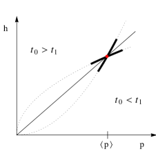
In the vicinity of the average value of $p$ the function $h(p)$ is approximately affine, hence we may expand

$$h=t_{0}\langle p\rangle+t_{1}(p-\langle p\rangle)+{\cal O}\left((p-\langle p\rangle)^{2}\right),$$ (3)

where $t_{i}$ are parameters depending on the dynamical response of hydrodynamics to the initial condition. The higher-order terms in Eq. (3) may be dropped if $p$ is sufficiently close to $\langle p\rangle$, otherwise corrections arise to the formulas developed below. With Eq. (3) we get

$$\langle h_{A}\rangle = t_{0}\langle p_{A}\rangle,$$

$$\langle\Delta h_{A}^{2}\rangle = t_{1}^{2}\langle\Delta p_{A}^{2}\rangle,$$

$$\langle\Delta h_{A}\Delta h_{A^{\prime}}\rangle = t_{1}^{2}\langle\Delta p_{A}\Delta p_{A^{\prime}}\rangle,$$

$$\langle\Delta h_{A}^{3}\rangle = t_{1}^{3}\langle\Delta p_{A}^{3}\rangle,$$ (4)

$$\langle\Delta h_{A}\Delta h_{A^{\prime}}^{2}\rangle = t_{1}^{3}\langle\Delta p_{A}\Delta p_{A^{\prime}}^{2}\rangle,$$

$$\langle\Delta h_{F}\Delta h_{C}\Delta h_{B}\rangle = t_{1}^{3}\langle\Delta p_{F}\Delta p_{C}\Delta p_{B}\rangle.$$

We note that the approximate linearity of the hydrodynamic response has been well determined for the evolution of eccentricities Gardim:2011xv ; Niemi:2012aj at a given centrality. For the present case of multiplicities, the success of modeling of the measured particle multiplicity distributions within the Glauber framework Back:2001xy ; Back:2004dy indirectly supports the assumptions leading to Eq. (4).

II.5 Statistical hadronization

When hydrodynamic evolution ends, statistical hadronization phase takes over at freeze-out (cf. Fig. 1). We assume that the well-separated fluid cells $h$ emit $n$ hadrons independently from one other into corresponding well-separated phase-space regions in pseudorapidity. Each of the $h$ cells emits $m$ hadrons in the same universal manner, hence

$$n_{A}=\sum_{i=1}^{h_{A}}m_{i}.$$ (5)

Then, in full analogy to Eq. (2), we obtain

$$\langle n_{A}\rangle = \langle m\rangle\langle h_{A}\rangle,$$

$$\langle\Delta n_{A}\rangle^{2} = {\rm var}(m)\langle h_{A}\rangle+\langle m\rangle^{2}\langle\Delta h_{A}\rangle^{2},$$

$$\langle\Delta n_{A}\Delta n_{A^{\prime}}\rangle = \langle m\rangle^{2}\langle\Delta h_{A}\Delta h_{A^{\prime}}\rangle,$$ (6)

$$\langle\Delta n^{3}_{A}\rangle = \mu_{3}\left(m\right)+3{\rm var}(m)\langle m\rangle\langle\Delta h_{A}^{2}\rangle$$

$$+ \langle m\rangle^{3}\langle\Delta h_{A}^{3}\rangle,$$

$$\langle\Delta n_{A}\Delta n^{2}_{A^{\prime}}\rangle = {\rm var}(m)\langle m\rangle\langle\Delta h_{A}\Delta h_{A^{\prime}}\rangle$$

$$+ \langle m\rangle^{3}\langle\Delta h_{A}\Delta h^{2}_{A^{\prime}}\rangle,$$

$$\langle\Delta n_{F}\Delta n_{C}\Delta n_{B}\rangle = \langle m\rangle^{3}\langle\Delta h_{F}\Delta h_{C}\Delta h_{B}\rangle.$$

The numbers $n_{A}$ are observed experimentally. We note that the distribution of $m_{i}$ incorporates the effects of the detector acceptance.

II.6 Combined formulas

We are now ready to combine Eqs. (2,4,6), which yield relations between moments of produced hadron distributions and moments of the initial sources:

$$\langle n_{A}\rangle = \alpha\langle s_{A}\rangle,$$

$$\langle\Delta n_{A}^{2}\rangle = \beta\langle s_{A}\rangle+\gamma\langle\Delta s_{A}^{2}\rangle$$

$$\langle\Delta n_{A}\Delta n_{A^{\prime}}\rangle = \gamma\langle\Delta s_{A}\Delta s_{A^{\prime}}\rangle,$$ (7)

$$\langle\Delta n_{A}^{3}\rangle = \zeta\langle s_{A}\rangle+3\gamma^{1/2}\beta^{\prime}\langle\Delta s_{A}^{2}\rangle+\gamma^{3/2}\langle\Delta s_{A}^{3}\rangle,$$

$$\langle\Delta n_{A}\Delta n_{A^{\prime}}^{2}\rangle = \gamma^{1/2}\beta^{\prime}\langle\Delta s_{A}\Delta s_{A^{\prime}}\rangle+\gamma^{3/2}\langle\Delta s_{A}\Delta s_{A^{\prime}}^{2}\rangle,$$

$$\langle\Delta n_{F}\Delta n_{C}\Delta n_{B}\rangle = \gamma^{3/2}\langle\Delta s_{F}\Delta s_{C}\Delta s_{B}\rangle.$$

The constants introduced above are defined as

$$\alpha = t_{0}\langle\mu\rangle\langle m\rangle,$$

$$\beta = t_{0}\langle\mu\rangle{\rm var}(m)+t_{1}^{2}\langle m\rangle^{2}{\rm var}(\mu),$$ (8)

$$\beta^{\prime} = t_{1}\langle\mu\rangle{\rm var}(m)+t_{1}^{2}\langle m\rangle^{2}{\rm var}(\mu),$$

$$\gamma = t_{1}^{2}\langle m\rangle^{2}\langle\mu\rangle^{2},$$

$$\zeta = t_{0}\mu_{3}(m)\langle\mu\rangle+3t_{1}^{2}{\rm var}(\mu){\rm var}(m)\langle m\rangle+t_{1}^{3}\mu_{3}(\mu)\langle m\rangle^{3}.$$

The algebraic structure of Eqs. (7) is very simple. However, nontrivial character stems from the fact that the parameters (8) do not depend on centrality of the collision.

It is convenient to introduce a short-hand notation

$$S_{ijk}=\langle\Delta s_{B}^{i}\Delta s_{C}^{j}\Delta s_{F}^{k}\rangle$$ (9)

for the moments of rank $r=i+j+k$, and

$$\tilde{S}_{ijk}=\frac{\langle\Delta s_{B}^{i}\Delta s_{C}^{j}\Delta s_{F}^{k}\rangle}{\sqrt{\langle\Delta s_{B}^{2}\rangle\langle\Delta s_{C}^{2}\rangle\langle\Delta s_{F}^{2}\rangle}}$$ (10)

for the moments scaled with the standard deviations. In particular, the forward-backward correlation of the number of sources is

$$\tilde{S}_{101} \equiv \frac{\langle\Delta s_{B}\Delta s_{F}\rangle}{\sqrt{\langle\Delta s_{B}^{2}\rangle\langle\Delta s_{F}^{2}\rangle}}\equiv\rho(s_{F},s_{B}).$$ (11)

The scaled variance, used in the following, is defined as

$$\omega(x_{A})={\rm var}(x_{A})/\langle x_{A}\rangle.$$ (12)

We also introduce the combinations of parameters

$$\delta = \beta/\alpha=\omega(m)+\frac{t_{1}^{2}}{t_{0}}\langle m\rangle\omega(\mu),$$

$$\kappa = \gamma/\alpha=\frac{t_{1}^{2}}{t_{0}}\langle\mu\rangle\langle m\rangle,$$ (13)

$$\lambda = \beta/\gamma=\frac{t_{0}\omega(m)}{t_{1}^{2}\langle\mu\rangle\langle m\rangle}+\frac{\omega(\mu)}{\langle\mu\rangle}.$$

III General results

III.1 Relations of moments of hadrons to moments of sources

Our methodology uses the Glauber model for the sources to make predictions for the moments of $n_{A}$.

An interesting relation for the hadron correlations results from Eq. (7):

$$\rho(n_{A},n_{A^{\prime}})={\rho(s_{A},s_{A^{\prime}})}{\sqrt{\left({1-\frac{\delta}{\omega(n_{A})}}\right)\left({1-\frac{\delta}{\omega(n_{A^{\prime}})}}\right)}}.$$

(14)

Since, as we shall see, for not too large pseudorapidity separations, in the Glauber model to a high accuracy $\rho(s_{A},s_{A^{\prime}})\simeq 1$, it then follows that

$$\rho(n_{A},n_{A^{\prime}})\simeq{\sqrt{\left({1-\frac{\delta}{\omega(n_{A})}}\right)\left({1-\frac{\delta}{\omega(n_{A^{\prime}})}}\right)}}.$$ (15)

which means a very specific relation between the correlation of numbers of hadrons in bins $A$ and $A^{\prime}$ and the corresponding scaled variances, which depends on a single centrality independent parameter $\delta$. Relation (15) may be straightforwardly tested with the future data.

From Eqs. (7) we also find

$$\omega(n_{A}) = \delta+\kappa\omega(s_{A}),$$

$$\rho(n_{F},n_{B}) \equiv \frac{\rho(s_{F},s_{B})}{\sqrt{\left(1+\frac{\lambda}{\omega(s_{F})}\right)\left(1+\frac{\lambda}{\omega(s_{B})}\right)}},$$ (16)

formulas presented already in Ref. Olszewski:2013qwa .

Another interesting relation, linking three bins, has the form

$$\frac{\langle\Delta n_{B}\Delta n_{C}\Delta n_{F}\rangle}{\langle\Delta n_{A}\Delta n_{A^{\prime}}\rangle^{3/2}}=\frac{\langle\Delta s_{B}\Delta s_{C}\Delta s_{F}\rangle}{\langle\Delta s_{A}\Delta s_{A^{\prime}}\rangle^{3/2}}.$$ (17)

Again, the right-hand side, obtainable in a model, can be verified against the future data, yielding the left-hand side.

With the help of the basic formulas (7) it is straightforward to find relations for the newly-proposed measures Gorenstein:2011vq ; Gazdzicki:2013ana of fluctuations. They are defined as

$$\Sigma(n_{F},n_{B}) = \frac{\langle n_{F}\rangle\omega(n_{B})+\langle n_{B}\rangle\omega(n_{F})-2{\rm cov}(n_{F},n_{B})}{C_{\Sigma}},$$

$$\Delta(n_{F},n_{B}) = \frac{\langle n_{B}\rangle\omega(n_{F})-\langle n_{F}\rangle\omega(n_{B})}{C_{\Delta}},$$ (18)

where the constants $C_{\Sigma}$ and $C_{\Delta}$ are proportional to first moments of any extensive quantity. We take the simplest choice

$$C_{\Sigma}=C_{\Delta}=\langle n_{F}\rangle+\langle n_{B}\rangle.$$ (19)

Elementary algebra leads to the relations

$$\Sigma(n_{F},n_{B}) = \delta+\kappa\Sigma(s_{F},s_{B}),$$

$$\Delta(n_{F},n_{B}) = \delta\frac{\langle s_{F}-s_{B}\rangle}{\langle s_{F}+s_{B}\rangle}+ \kappa\Delta(s_{F},s_{B}),$$ (20)

where $\Sigma(n_{F},n_{B})$ and $\Delta(n_{F},n_{B})$ are defined analogously to Eq. (18), but with $n_{A}$ replaced with $s_{A}$.

III.2 Implications for the qualitative features of hydrodynamics

Based on first and third of Eqs. (7), we find the relation

$$\frac{t_{0}}{t_{1}}=\frac{\alpha}{\gamma^{1/2}}.$$ (21)

Since the $\alpha$ and $\gamma$ parameters may be found by fitting the model predictions to the future data, we are able to obtain from Eq. (21) information concerning the hydrodynamic response in the intermediate phase. Figure (3) shows two possible scenarios for the hydro evolution. When $t_{0}>t_{1}$ ($t_{0}<t_{1}$), the hydrodynamic growth $h(p)$ is slower (faster) than the linear function. From the experience of hydrodynamics we expect that $t_{0}\simeq t_{1}$, which means that the entropy in the considered cell is proportional to its initial entropy (see, e.g., Bozek:2011ua ).

Figure 3: (color online) Possible scenarios for the hydrodynamic response (see text for details).

IV Dependence of results on width of centrality bins

An important question concerns the dependence of the results shown in this paper on centrality selection. In our analysis presented below we define centrality with the help of the number of sources in the central bin, $s_{C}$. The results for moments of multiplicities depend on the chosen width of the centrality bin $\Delta c$ – in that sense they are not intensive measures Gorenstein:2011vq ; Mrowczynski:1999un . Nevertheless, the moments evaluated that way are still useful for comparing model predictions to experiment, as exactly the same choice of width of the centrality windows can be made in model simulations as in the data analysis.

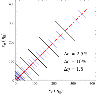
To understand the problem, let us focus on Fig. 4, where we show a result of a simulation in the form of a scattered plot of $s_{F}$ and $s_{B}$. The short skewed lines cut the events into subsequent centrality classes with $\Delta c=2.5\%$, while the longer lines into classes with $\Delta c=10\%$ (containing 4 bins of $\Delta c=2.5\%$). We note that the scattered plot is very much elongated, simply reflecting the large correlation between $s_{F}$ and $s_{B}$. With the exception of very small centralities $c$ (the lower left corner of the plot), the correlation between $s_{F}$ and $s_{B}$ within a given centrality window is very close to 1, $\rho(s_{F},s_{B})\simeq 1$. As we move towards very low $c$ (lower-left corner), or when $\Delta c$ is decreased, $\rho(s_{F},s_{B})$ becomes lower than 1. Thus the correlation of the sources is in an obvious way affected by the choice of the centrality bins.

For sufficiently large width of the bins, the above-discussed feature allows us for a derivation of approximate scaling laws of the moments on $\Delta c$. Details are shown in Appendix A. The average multiplicities do not scale, as long as the window is sufficiently narrow:

$$\langle s_{A}\rangle\sim(\Delta c)^{0}.$$ (22)

For the variance and covariance we find

$$\langle(\Delta s_{A})^{2}\rangle\sim(\Delta c)^{2},$$

$$\langle\Delta s_{A}\Delta s_{A^{\prime}}\rangle\sim(\Delta c)^{2},$$ (23)

from where

$$\rho(s_{A},s_{A^{\prime}})\sim(\Delta c)^{0}.$$ (24)

For the moments of rank 3 we need to be a bit more sophisticated. The marginal distribution for the variable $s_{A}$ in a given centrality bin can be approximated as an affine function, $f(s_{A})=N(1+as_{A})$, where $a$ is small. Then (cf. Appendix A), to leading order in $a$

$$\langle(\Delta s_{A})^{3}\rangle\sim a(\Delta c)^{4},$$ (25)

and

$$\langle(\Delta s_{A})^{3}\rangle/\langle\Delta s_{A}\Delta s_{A^{\prime}}\rangle^{3/2}\sim a\Delta c.$$ (26)

The above scaling laws are visible in our results presented below.

Figure 4: (color online) Scattered plot for the forward-backward correlation of the numbers of initial sources $s_{F}$ and $s_{B}$ for rapidity separation $\Delta\eta=1.8$. The short lines cut the sample into centrality bins of width $\Delta c=2.5\%$, and the long lines into bins of width $\Delta c=10\%$. GLISSANDO, mixed model, Pb+Pb collisions at the LHC energy of $\sqrt{s_{NN}}=2.76\textrm{ TeV}$.

V GLISSANDO simulations

We use GLISSANDO Rybczynski:2013yba to model the initial phase. To simulate Pb+Pb collisions at the LHC at $\sqrt{s_{NN}}=2.76\textrm{ TeV}$, we use (unless stated otherwise) the mixed Glauber model  Kharzeev:2000ph ; SchaffnerBielich:2001qj ; Back:2001xy with the mixing parameter $a=0.1$ (cf. Appendix B), the NN cross section $\sigma_{NN}=66.3\textrm{ mb}$ and a Gaussian wounding profile Rybczynski:2011wv . The numbers of sources $s_{A}$ are obtained in pseudo-rapidity bins of width $\delta\eta=0.2$, while $\Delta\eta$ denotes the separation of the centers of the $F$ and $B$ bins. The $C$ bin is centered around zero, while the $F$ and $B$ bins are arranged symmetrically.

Figure 5: (color online) Forward-backward and forward-central correlations of the number of initial sources, plotted as functions of centrality for two cases of the pseudorapidity separation, $\Delta\eta=1.8$ and $\Delta\eta=10$.

Figure 6: (color online) Scaled rank-3 moments of sources plotted as functions of centrality for three sample values of the width for the centrality bins.

V.1 Results for the correlations of sources

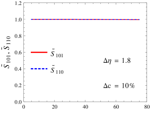
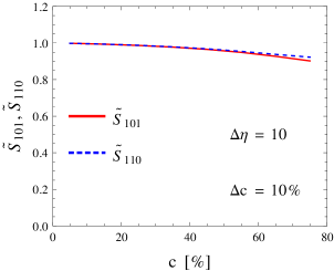
We begin presenting our results with the forward-backward and forward-central correlation functions, $\tilde{S}_{101}$ and $\tilde{S}_{110}$, shown in Fig. 5 for the rapidity separations $\Delta\eta=1.8$ and $\Delta\eta=10$. We use $\Delta c=10$ %, but as follows from Eq. (23), the results are insensitive to the width of the bin. We note that these correlation functions are essentially equal to unity, except for very large values of $\Delta\eta$ and $c$. This is an interesting feature of the adopted Glauber model, as it shows that we can use $\rho(s_{A},s_{A^{\prime}})\simeq 1$ in practical applications. This fact has its origin in a strong correlation between the numbers of wounded nucleons from nuclei A and B, as well as between the wounded nucleons and the binary collisions (cf. Appendix B).

For the case of symmetric collisions and symmetrically placed F and B bins, the measures $\Sigma(s_{F},s_{B})$ and $\Delta(s_{F},s_{B})$ from Eq. (18) are equal to

$$\Sigma(s_{F},s_{B}) = \omega(s_{A})[1-\rho(s_{F},s_{B})],$$ (27)

$$\Delta(s_{F},s_{B}) = 0,\hskip 85.35826pt(A=F,B),$$

Since $\rho(s_{F},s_{B})\simeq 1$, it follows that $\Sigma(s_{F},s_{B})\simeq 0$.

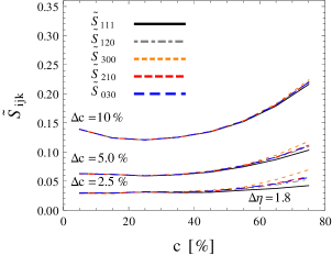
The scaled rank-3 correlations of Eq. (10) are displayed in Fig. 6. We note the advocated scaling with the value of $\Delta c$, cf. Eq. (26). Moreover, various rank-3 moments shown in the plot are essentially equal to one another in the Glauber treatment.

Figure 7: (color online) Prediction for the combination of third and second moments of observed hadrons, plotted as a function of centrality for three pseudo-rapidity separations, $\Delta\eta=1.8,\ 6,\ 10$.

V.2 Results for the correlations of produced hadrons

Figure 8: (color online) Same as in Fig. 7, but for different variants of the Glauber model.

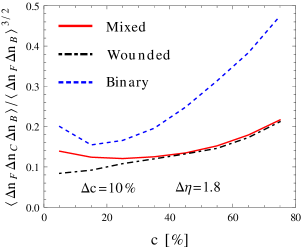
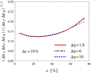
Now we pass to the presentation of results for the moments of the distributions of the produced hadrons, $n_{A}$. Under the assumptions of the superposition approach, Eq. (17) allows us to make predictions for the produced hadrons, based on the model of sources. Our result, for several pseudo-rapidity separations $\Delta\eta$, is shown in Fig. 7. The result is specific to the adopted source production model. In Fig. 8 we compare the outcome, for the same quantity, of the wounded nucleon model (mixing parameter $a=0$), the mixed model ($a=0.1$), and the binary-collisions model ($a=1$). The large differences between the models should allow, with the future data, to discriminate between them.

Figure 9: (color online) Predictions for the multiplicity of the produced hadrons in peripheral bins, plotted as a functions of centrality, based on Eq. (7) at different values of parameters in Eq. (8,13).

Figure 10: (color online) Same as Fig. 9, but for the variance.

Figure 11: (color online) Same as Fig. 9, but for the scaled variance.

Figure 12: (color online) Same as Fig. 9, but for the covariance.

Figure 13: (color online) Same as Fig. 9, but for the forward-backward correlations.

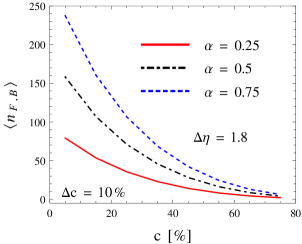
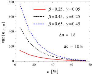
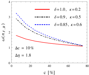
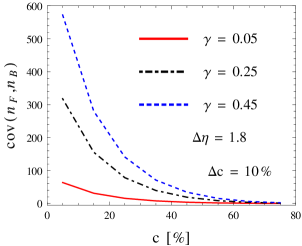
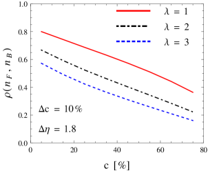
Finally, we use Eq. (7) with some reasonable choice of the parameters (8,13) to make predictions for the multiplicity, variance, covariance, and rank-2 correlation coefficients. The results are displayed in Figs. 9-13. We may now carefully illustrate our methodology: with the data for multiplicity we fit the value of $\alpha$ with the results of Fig. 9, the value of $\gamma$ with Fig. 12, and then the value of $\beta$ with Fig. 10. Next, we evaluate $\lambda=\beta/\gamma$ and make a test with the help of Fig. 13. Extension to rank-3 moments is straightforward. That way, we may obtain the parameters of the superposition model in a systematic way. Knowledge of these parameters will provide insight into the microscopic features of the particle production mechanism in the system.

V.3 Centrality from the number of hadrons

In this Section we check how the results for the forward-backward correlations depend on the method of determining centrality, carrying out a study similar to Ref. Konchakovski:2008cf . In Sec. II.2 we have introduced the definition of centrality, used in the remaining parts of this paper, based on the number of sources in the central rapidity bin, $s_{C}$. To estimate the results based on centrality determined with number of produced hadrons in the central bin, $n_{C}$, we carry out GLISSANDO simulations, where a negative binomial distribution is superimposed over the distribution of sources. The parameters of the binomial distributions are such that the experimental multiplicity distributions at the LHC are reproduced Bozek:2015bna .

The qualitative effect of the superimposed fluctuations is simple to understand: when the limits of the centrality bin are $n_{C}^{\rm low}$ and $n_{C}^{\rm high}$, the corresponding limits in the number of sources, $s_{C}^{\rm low}$ and $s_{C}^{\rm high}$ are somewhat diffused. This causes more extended scattered plot of type of Fig. 4 for the events belonging to the considered centrality class and the correlation coefficient $\rho(s_{F},s_{B})$ increases. As may be inferred form Fig. 4, the effect will be larger for peripheral collisions, where the scattered plots are less elongated, and smaller for central collisions, where elongation (for $\Delta c=10\%)$ is large.

Figure 14: (color online) Influence of the method of centrality selection for the forward-backward correlation of sources, tested with the ratio $\tilde{S}_{101}/\tilde{S}^{\rm NB}_{101}$ of the forward-backward correlations evaluated with the number of sources $s_{C}$ and the number of hadron $n_{C}$ in the central rapidity bin. At small forward-backward separation, $\Delta\eta=1.8$, there is no effect of the method used to determine centrality.

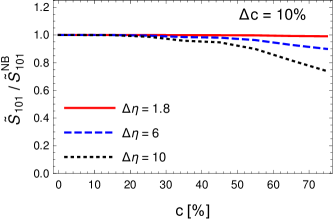
Results of our numerical simulations are presented in Fig. 14, where we show the ratio of the correlation coefficients $\tilde{S}_{101}$ for the centralities evaluated according to $s_{C}$ and according to $n_{C}$ obtained with the overlaid negative binomial distribution, indicated as $\tilde{S}_{101}/\tilde{S}^{\rm NB}_{101}$. We note that for small forward-backward pseudorapidity separation, $\Delta\eta=1.8$, there is no visible effect, whence $\tilde{S}_{101}/\tilde{S}^{\rm NB}_{101}\simeq 1$. For large $\Delta\eta$ and peripheral collisions $\tilde{S}_{101}/\tilde{S}^{\rm NB}_{101}<1$, in agreement with the qualitative arguments presented above.

VI Conclusions

We have presented a systematic study of two- and three-rapidity-bin multiplicity correlations in relativistic heavy-ion collisions in a superposition approach, based on three phases of the collision: initial partonic phase, intermediate collective evolution, and final statistical hadronization. The derived expressions show how the moments of the produced particles are related to the moments of the sources produced in the initial phase. The relations, simple but nontrivial, involve only a few parameters collecting the microscopic information concerning the dynamics (parameters of the superimposed distributions, response of hydrodynamics).

With a definite model for the production of sources, such as the Glauber model used here, one is then able to obtain in a systematic way predictions for the multibin multiplicity correlations of the produced hadrons. Conversely, with the future experimental data, one will be able to test the models of the initial phase, as well as obtain information on the microscopic parameters. In particular, the awaited forward-backward multiplicity correlation analysis with the LHC data will shed light on the early production mechanism. The statistical method presented in this paper is directly applicable to that case.

Appendix A Centrality width dependence

In this Appendix we sketch the derivation of scaling of the moments with the width of the centrality bin. The explanation comes from Fig. (4), where the forward-backward correlation is plotted as scattered plot. For a given centrality and for a typical size of $\Delta c$ we may approximate the distribution of $s_{A}=x$ as an affine function,

$$f(x) = \frac{1+ax}{\left(1+ac\right)\Delta c},$$ (28)

which has been normalize to 1. Upon expanding for small $ac$ it follows that

$$\langle x\rangle=\int_{c-\frac{\Delta c}{2}}^{c+\frac{\Delta c}{2}}xf(x)\simeq c+\frac{a\Delta c^{2}}{12},$$ (29)

$$\langle\left(\Delta x\right)^{2}\rangle=\int_{c-\frac{\Delta c}{2}}^{c+\frac{\Delta c}{2}}\left(x-\langle x\rangle\right)^{2}\simeq\frac{\Delta c^{2}}{12},$$

$$\langle\left(\Delta x\right)^{3}\rangle=\int_{c-\frac{\Delta c}{2}}^{c+\frac{\Delta c}{2}}\left(x-\langle x\rangle\right)^{3}\sim\Delta c^{4},$$

$$\frac{\langle\left(\Delta x\right)^{3}\rangle}{\langle\left(\Delta x\right)^{2}\rangle^{3/2}}\sim\Delta c.$$

The scaling laws (22,23) result from the above formulas.

Appendix B Emission profiles in spatial rapidity

Figure 15: (color online) The emission profiles in space-time rapidity for the wounded nucleons (dashed lines) and the binary collisions (solid line). The profile $f_{+}(f_{-})$ corresponds to the forward (backward) moving wounded nucleons.

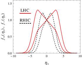
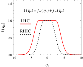
In a nucleus-nucleus collision, the emission profile Bozek:2010bi defining the shape of initial sources in the spatial rapidity has the form

$$s\!\left(\eta_{||}\right) = \left(\frac{1-a}{2}\right)\left(f_{+}\!\left(\eta_{||}\right)N_{w,B}+f_{-}\!\left(\eta_{||}\right)N_{w,F}\right)$$ (30)

$$+ a\left(\frac{f_{+}\!\left(\eta_{||}\right)+f_{-}\!\left(\eta_{||}\right)}{2}\right)N_{bin},$$

where $N_{w,F}$ and $N_{w,F}$ are the numbers of the forward- and backward-going wounded nucleons, $N_{bin}$ is the number of binary collisions, while $f_{+}\left(\eta_{||}\right)$ and $f_{-}\left(\eta_{||}\right)$ describe the corresponding wounded-nucleon emission profiles. Finally, $f\left(\eta_{||}\right)$ is the emission profile for the binary collisions. We use the following parametrization Bozek:2010bi :

$$f\left(\eta_{||}\right) = \exp\!\left(-\frac{\left(|\eta_{||}|-\eta_{0}\right)^{2}}{2\sigma^{2}}\theta\!\left(|\eta_{||}|-\eta_{0}\right)\right),$$

$$f_{+}\left(\eta_{||}\right) = f_{F}\left(\eta_{||}\right)f\left(\eta_{||}\right),$$ (31)

$$f_{-}\left(\eta_{||}\right) = f_{F}\left(-\eta_{||}\right)f\left(\eta_{||}\right),$$

with

$$f_{F}\left(\eta_{||}\right)=\left\{\begin{array}[]{ll}0,&\eta_{||}\leq-\eta_{m}\\ \frac{\eta_{||}+\eta_{m}}{2\eta_{m}}&-\eta_{m}<\eta_{||}<\eta_{m}\\ 1&\eta_{m}\leq\eta_{||}.\end{array}\right.$$

Sample values of parameters Bozek:2013uha , describing the ATLAS data after the hydrodynamic evolution, are $\eta_{0}=1.25$, $\eta_{m}=8.58$, $\sigma_{\eta}=1.4$. The functions (31) are shown in Fig. 15.

References

- (1) S. Uhlig, I. Derado, R. Meinke, and H. Preissner, Nucl. Phys. B132, 15 (1978)
- (2) K. Alpgard et al. (UA5), Phys. Lett. B123, 361 (1983)
- (3) R. E. Ansorge et al. (UA5), Z. Phys. C37, 191 (1988)
- (4) T. Alexopoulos et al. (E735), Phys. Lett. B353, 155 (1995)
- (5) B. I. Abelev et al. (STAR), Phys. Rev. Lett. 103, 172301 (2009)
- (6) T. J. Tarnowsky, Proceedings, 26th Winter Workshop on Nuclear Dynamics (WWND 2010), J. Phys. Conf. Ser. 230, 012025 (2010)
- (7) G. Aad et al. (ATLAS), JHEP 07, 019 (2012)
- (8) A. Capella and A. Krzywicki, Phys. Rev. D18, 4120 (1978)
- (9) N. S. Amelin, N. Armesto, M. A. Braun, E. G. Ferreiro, and C. Pajares, Phys. Rev. Lett. 73, 2813 (1994)
- (10) M. A. Braun, C. Pajares, and V. V. Vechernin, Phys. Lett. B493, 54 (2000)
- (11) M. A. Braun, R. S. Kolevatov, C. Pajares, and V. V. Vechernin, Eur. Phys. J. C32, 535 (2004)
- (12) P. Brogueira, J. Dias de Deus, and J. G. Milhano, Phys. Rev. C76, 064901 (2007)
- (13) N. Armesto, M. A. Braun, and C. Pajares, Phys. Rev. C75, 054902 (2007)
- (14) N. Armesto, L. McLerran, and C. Pajares, Nucl. Phys. A781, 201 (2007)
- (15) V. V. Vechernin and R. S. Kolevatov, Phys. Atom. Nucl. 70, 1797 (2007), [Yad. Fiz.70,1846(2007)]
- (16) M. A. Braun, Nucl. Phys. A806, 230 (2008)
- (17) V. P. Konchakovski, M. Hauer, G. Torrieri, M. I. Gorenstein, and E. L. Bratkovskaya, Phys. Rev. C79, 034910 (2009)
- (18) A. Bzdak and K. Wozniak, Phys. Rev. C81, 034908 (2010)
- (19) T. Lappi and L. McLerran, Nucl. Phys. A832, 330 (2010)
- (20) P. Bozek, W. Broniowski, and J. Moreira, Phys. Rev. C83, 034911 (2011)
- (21) J. Dias de Deus and C. Pajares, Phys. Lett. B695, 211 (2011)
- (22) A. Bzdak, Phys. Rev. C85, 051901 (2012)
- (23) A. Bzdak and D. Teaney, Phys. Rev. C87, 024906 (2013)
- (24) V. V. Vechernin(2012), arXiv:1210.7588 [hep-ph]
- (25) A. Bialas, A. Bzdak, and K. Zalewski, Acta Phys.Polon.Supp. 6, 463 (2013)
- (26) S. De, T. Tarnowsky, T. K. Nayak, R. P. Scharenberg, and B. K. Srivastava, Phys. Rev. C88, 044903 (2013)
- (27) G.-L. Ma and A. Bzdak, Phys. Lett. B739, 209 (2014)
- (28) A. Bialas and K. Zalewski, Nucl. Phys. A860, 56 (2011)
- (29) A. Bialas and K. Zalewski, Phys. Lett. B698, 416 (2011)
- (30) A. Olszewski and W. Broniowski, Phys.Rev. C88, 044913 (2013)
- (31) A. Bialas, M. Bleszynski, and W. Czyz, Nucl. Phys. B111, 461 (1976)
- (32) A. Bialas, Strangeness in quark matter. Proceedings, International Conference, SQM 2007, Levoca, Slovakia, June 24-29, 2007, J. Phys. G35, 044053 (2008)
- (33) W. Broniowski, P. Bozek, and M. Rybczynski, Phys. Rev. C76, 054905 (2007)
- (34) D. Kharzeev and M. Nardi, Phys. Lett. B507, 121 (2001)
- (35) J. Schaffner-Bielich, D. Kharzeev, L. D. McLerran, and R. Venugopalan, Nucl. Phys. A705, 494 (2002)
- (36) B. B. Back et al. (PHOBOS), Phys. Rev. C65, 031901 (2002)
- (37) W. Ehehalt and W. Cassing, Nucl. Phys. A602, 449 (1996)
- (38) W. Czyz and L. C. Maximon, Annals Phys. 52, 59 (1969)
- (39) A. Kovner, L. D. McLerran, and H. Weigert, Phys. Rev. D52, 6231 (1995)
- (40) E. Iancu, A. Leonidov, and L. D. McLerran, Nucl. Phys. A692, 583 (2001)
- (41) T. Lappi, High energy strong interactions. Proceedings, International Symposium, HESI10, Kyoto, Japan, August 9-13, 2010, Prog. Theor. Phys. Suppl. 187, 134 (2011)
- (42) T. Lappi, Proceedings, Workshop for Young Scientists on the Physics of Ultrarelativistic Nucleus-Nucleus Collisions (Hot Quarks 2010), J. Phys. Conf. Ser. 270, 012055 (2011)
- (43) P. Brogueira and J. Dias de Deus, Phys. Lett. B653, 202 (2007)
- (44) U. Heinz and R. Snellings, Ann.Rev.Nucl.Part.Sci. 63, 123 (2013)
- (45) C. Gale, S. Jeon, and B. Schenke, Int.J.Mod.Phys. A28, 1340011 (2013)
- (46) Z.-W. Lin, C. M. Ko, B.-A. Li, B. Zhang, and S. Pal, Phys. Rev. C72, 064901 (2005)
- (47) W. Florkowski, Phenomenology of Ultra-Relativistic Heavy-Ion Collisions (World Scientific Publishing Company, Singapore, 2010)
- (48) R. J. Glauber in Lectures in Theoretical Physics W. E. Brittin and L. G. Dunham eds., (Interscience, New York, 1959) Vol. 1, p. 315
- (49) M. L. Miller, K. Reygers, S. J. Sanders, and P. Steinberg, Ann. Rev. Nucl. Part. Sci. 57, 205 (2007)
- (50) P. Bozek and I. Wyskiel, Phys. Rev. C81, 054902 (2010)
- (51) A. Bialas and W. Czyz, Acta Phys. Polon. B36, 905 (2005)
- (52) R. Nouicer et al. (PHOBOS), Ultra-relativistic nucleus-nucleus collisions. Proceedings, 17th International Conference, Quark Matter 2004, Oakland, USA, January 11-17, 2004, J. Phys. G30, S1133 (2004)
- (53) M. Gazdzicki and M. I. Gorenstein, Phys. Lett. B640, 155 (2006)
- (54) A. Bzdak, Phys. Rev. C80, 024906 (2009)
- (55) D. Kharzeev, E. Levin, and M. Nardi, Nucl. Phys. A730, 448 (2004), [Erratum: Nucl. Phys.A743,329(2004)]
- (56) H.-J. Drescher, A. Dumitru, A. Hayashigaki, and Y. Nara, Phys. Rev. C74, 044905 (2006)
- (57) J. I. Kapusta, B. Muller, and M. Stephanov, Phys. Rev. C85, 054906 (2012)
- (58) J. Kapusta, B. Muller, and M. Stephanov, Proceedings, International Conference on Strangeness in Quark Matter (SQM 2011), Acta Phys. Polon. B43, 781 (2012)
- (59) F. G. Gardim, F. Grassi, M. Luzum, and J.-Y. Ollitrault, Phys. Rev. C85, 024908 (2012)
- (60) H. Niemi, G. Denicol, H. Holopainen, and P. Huovinen, Phys.Rev. C87, 054901 (2013)
- (61) B. B. Back et al. (PHOBOS), Phys. Rev. C70, 021902 (2004)
- (62) M. I. Gorenstein and M. Gazdzicki, Phys. Rev. C84, 014904 (2011)
- (63) M. Gazdzicki, M. Gorenstein, and M. Mackowiak-Pawlowska, Phys.Rev. C88, 024907 (2013)
- (64) P. Bozek, Phys. Rev. C85, 034901 (2012)
- (65) S. Mrowczynski, Phys. Lett. B465, 8 (1999)
- (66) M. Rybczynski, G. Stefanek, W. Broniowski, and P. Bozek, Comput. Phys. Commun. 185, 1759 (2014)
- (67) M. Rybczynski and W. Broniowski, Phys. Rev. C84, 064913 (2011)
- (68) P. Bozek and W. Broniowski(2015), arXiv:1506.02817 [nucl-th]
- (69) P. Bozek and W. Broniowski, Phys.Rev. C88, 014903 (2013)