Performance Estimation for Two-Dimensional Brownian Rotary Ratchet Systems

Abstract

Within the context of the Brownian ratchet model, a molecular rotary system was studied that can perform unidirectional rotations induced by linearly polarized ac fields, and produce positive work under loads. The model is based on the Langevin equation for a particle in a two-dimensional (2D) three-tooth ratchet potential of threefold symmetry. The performance of the system is characterized by the coercive torque, i.e., the strength of the load competing with the torque induced by the ac driving field, and the energy efficiency in force conversion from the driving field to torque. We propose a master equation for coarse-grained states, which takes into account boundary motion between states, and develop a kinetic description to estimate mean angular momentum (MAM) and powers relevant to the energy balance equation. The framework of analysis incorporates several 2D characteristics, and is applicable to a wide class of models of smooth 2D ratchet potential. We confirm that the obtained expressions for MAM, power, and efficiency of the model can predict qualitative behaviors. We also discuss the usefulness of the torque/power relationship for experimental analyses, and propose a characteristic for 2D ratchet systems.

1 Introduction

Standard internal combustion engines generate torque by burning fuel in the combustion chambers of cylinders. The kinetic energy of the expanding gases is applied to move a piston, which in turn is connected to a crankshaft to produce rotation and do work. The performance of an engine is specified by the maximum output power and torque and its energy (fuel) efficiency under certain conditions. Such characterizations can also be applied to biological molecular motors, a subject that has been of growing interest in recent biophysical research.

V- and F-type ATPases are examples of rotary molecular motors, which perform proton pumping or ATP synthesis to maintain cell activity (for a recent review, see Ref. NakanishiMatsui20101343). Surprisingly, they are similar in appearance to a Wankel engine, which mainly consists of a cylinder, a rotor, and an eccentric shaft and has three moving chambers for each stroke of a combustion cycle (intake, compression, ignition, and exhaust).[2] In the F₁ domain of ATPase, the so-called $\gamma$-shaft rotates inside a cylinder consisting of three symmetrically arranged, paired $\alpha$- and $\beta$-subunits. ATP is hydrolyzed to ADP and phosphate, with the released chemical bonding energy being spent to perform the rotation. [3, 4, 5] The conversion is known to be highly energy efficient.[6, 7]

Apart from their energy sources, a basic difference between biological and man-made engines may lie in the stiffness of their architectural components. For molecular motors, recent single-molecule analyses have begun to discover mechanisms involving local deformations in the cylinder unit caused by ATP hydrolysis that generate torque, which rotates the $\gamma$-shaft.[8] In contrast to such deformable components, the piston and cylinder in man-made engines are made of harder materials. For the latter, it is also known that efficient operation requires completely sealed combustion chambers, as well as bearings and lubricant to maintain smooth mechanical movement. However, in biological engines the relevance of such deformations among components to the efficiency of force conversion remains mysterious.

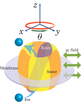
Figure 1: (Color online) Sketch of an AMM. The rod is loosely positioned inside the cylinder and can freely rotate around the $z$-axis. During rotation, its tilt with respect to the $z$-axis is maintained by contacts on the cylinder. The cylinder has three attachment points for the rod and works as a three-tooth ratchet. The cylinder is embedded in the membrane of a vesicle. When the rod rotates in a certain direction, the system can pump certain ions up and across the membrane. The $z$-axis of the Cartesian coordinate system is fixed to the axis of the cylinder. The arrows at right denote a linearly polarized ac field.

Our motivation is to understand the properties of the force-to-torque conversion in (artificial) molecular motors with deformable components when certain stimuli are applied, i.e., properties independent of energy sources, and our approach is based on mathematical modeling. In addition to biological molecular motors, artificial molecular motors (AMMs)[9, 10, 11, 12] represent good objects of study in this context. AMMs (or synthetic molecular motors) are small devices consisting of a rotor and stator consisting of (supra-) molecules, the rotor being capable of rotation relative to the stator under certain stimuli. Such rotation is largely due to noncovalent interactions between the rotor and stator. In particular, the recently described rotational, propeller-shaped supramolecules confined in nanopores[13] can be considered to be an example of an AMM made of deformable units. One significant advantage of studying AMMs is their well-characterized symmetry and responses to external stimuli. For more detailed information on AMMs, see the reviews in Refs. doi:10.1021/cr0300993,Browne2006,ANIE:ANIE200504313,ijms11062453.

Ratchet models [14] provide a basis for the theoretical study of molecular motors.[15, 16, 11, 17, 18, 19] In particular, a variety of one-dimensional (1D) piecewise linear ratchet models plays an important role in determining energy efficiency.[20, 21, 22, 23, 24, 25, 26] In the context of molecular rotary motors, these models treat the rotation of the rotor as the 1D motion of a particle in a sawtooth-type potential, and they demonstrate that a particle can move unidirectionally as a result of certain stimuli or modulations of the potential. Thus, ratchet models partly account for deformation of the cylinder subunit through modulation of the potential. However, realistic deformations are more complex than potential modulations in 1D space and involve richer dynamics. It therefore seems natural for our purpose to investigate the effects of two-dimensional potential modulations on efficiency with 2D ratchet models, as a minimal system of deformable units.

Figure 1 shows a schematic of the three-tooth rotary ratchet system that we consider as an AMM, which is composed of a rod (rotor) and cylinder (stator) and is anchored in and crosses a membrane. The system is perturbed by a heat bath and exposed to electromagnetic fields. The rod can respond to such fields and be driven by a linearly polarized ac field, which temporally modulates an effective potential for the rod–cylinder interaction. Here we assume that the polarization axis lies in the $xy$-plane (see Fig. 1 for the coordinate system).

Under certain conditions, the driving field can induce unidirectional rotation of the rotor in the stator. This can be used to generate work when a load is applied. As an example, we suppose that the system functions as a pump of ions across the membrane, against the concentration gradient. We focus on two main questions: How great a load can the driving field bear in performing productive work? How can the efficiency of the conversion of power from the ac field’s input to the output work be estimated?

Such systems have been studied in Refs. PhysRevE.84.061119 and PhysRevE.87.022144, where the rotor–stator interaction was described with 2D ratchet potentials having either twofold or threefold symmetry (two- or three-tooth rotary ratchet models) and the dynamics were analyzed using the Langevin equation for a particle in such potentials. The main interest was the robustness of the unidirectional rotation induced by a linearly polarized ac field. One result was that, unlike the two-tooth structure, the three-tooth ratchet allows robust unidirectional rotation for any polarization. However, loads and energy efficiency were not considered in those studies.

Here, to target these two questions, we develop a coarse-grained kinetic description that incorporates the deformational properties of 2D ratchet systems, through an analysis of the efficiency of force conversion from the ac driving field to the torque under load in the three-tooth rotary ratchet model. As a part of this framework, we propose a master equation, which is extended by taking into account the motion of boundaries between coarse-grained states. This enables us to estimate expectation values for the time derivatives of physical variables and to extract characteristic quantities related to the force conversion. The analytic expressions obtained for mean angular momentum, power, and efficiency agree qualitatively with numerical simulation data using a few adjustable parameters.

We describe our model in Sect. 2 and present its characteristic dynamics in Sect. 3. We propose the coarse-grained dynamical description in Sect. 4 and show the results for the energetics in Sect. 5. In Sect. 6, we discuss the relationship between mean angular momentum and output power and propose a characteristic feature of 2D ratchet systems.

2 Model

(a)	(b)

(c)	(d)

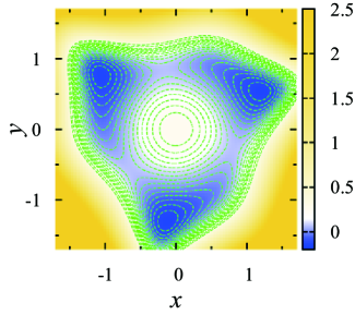
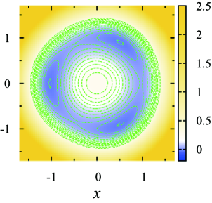
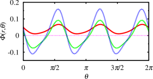
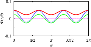
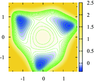
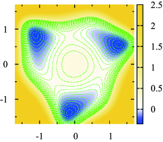
Figure 2: (Color online) Contour graphs of $V_{0}(\boldsymbol{x})$ and potential profiles. Panels (a) and (b) show the contour graphs of $V_{0}(\boldsymbol{x})$ at (a) $(a,b,c,d)=(-0.1,0.3,0.15,-0.1)$ and (b) $(-0.1,0,0.15,0)$, where the horizontal (vertical) direction corresponds to the $x$ ($y$) direction, and the dashed curves draw contour levels. Panels (c) and (d) show the curves of $\Phi(r,\theta)$ for the azimuthal angle $\theta\in[0,2\pi]$ at three radii $r\in\{0.8,1.0,1.1\}$. The values for $(a,b,c,d)$ of (c) and (d) are those of (a) and (b), respectively. The potential in panel (a) [(c)] is chiral with a ratchet structure, and that in panel (b) [(d)] is achiral without a ratchet structure. The ratchet direction of the potential in panel (a) [or (c)] is defined as anticlockwise (positive).

The rotational motion of the rotor tip in the stator (Fig. 1) is described as motion of a particle in a 2D ratchet potential. Consider the projection of the rotor tip onto the $xy$-plane. Let us describe its position at time $t$ as $\boldsymbol{X}(t)\equiv[X(t),Y(t)]^{{}^{\top}}$, the movement of $\boldsymbol{X}(t)$ (${\equiv}\boldsymbol{X}$) is described by the Langevin equation,

$$\gamma\dot{\boldsymbol{X}}(t)=-\partial_{\boldsymbol{X}}V(\boldsymbol{X},t)+\boldsymbol{R}(t)\quad(\gamma=1),$$ (1)

where $\partial_{\boldsymbol{x}}V\equiv(\partial V/\partial x,\partial V/\partial y)^{{}^{\top}}$, $\gamma$ is the viscous damping coefficient, which is set to unity, and $\boldsymbol{R}\equiv[R_{x}(t),R_{y}(t)]^{{}^{\top}}$ is the white Gaussian noise characterized by the ensemble averages $\langle R_{j}(t)\rangle=0$ and $\langle R_{j}(t)R_{k}(t^{\prime})\rangle=2D\delta_{j,k}\delta(t-t^{\prime})$, $j,k\in\{x,y\}$, with $D$ the strength of the noise. We regard $\boldsymbol{R}$ as thermal noise, and impose $D=\gamma k_{\mathrm{B}}T$, where $k_{\mathrm{B}}$ and $T$ are the Boltzmann constant and the temperature. $V(\boldsymbol{x},t)$ [${=}V_{0}(\boldsymbol{x})+V_{h}(\boldsymbol{x},t)+V_{I}(\boldsymbol{x})$] is the potential function. $V_{0}(\boldsymbol{x})$ represents a three-tooth ratchet potential [Figs. 2(a) and 2(b)]: in the 2D polar representation $\boldsymbol{x}^{{}^{\top}}=(r\cos\theta,r\sin\theta)$, $V_{0}(\boldsymbol{x})\equiv\Phi(r,\theta)$ reads

$$\Phi(r,\theta)=\Phi_{0}(r)-\frac{a}{4}r^{3}\cos 3\theta-\frac{b}{4}r^{5}\sin 3\theta+\frac{d}{6}r^{6}\sin 6\theta,$$ (2)

where $\Phi_{0}(r)=(1-r^{2})^{2}(1+cr^{2})/4$ [Figs. 2(c) and 2(d)]. $\Phi_{0}(r)$ builds a potential valley. This is modified from that in Ref. PhysRevE.87.022144 for a better confinement of motion within the valley. The second and third terms in Eq. (2) create the threefold symmetry. The fourth term makes a ratchet structure by adding asymmetry in azimuth. Below, we treat only potentials with three minima and saddles on the valley as in Figs. 2(a) and 2(b). $V_{h}(\boldsymbol{x},t)$ [${\equiv}\,\mathord{-}H(t)\boldsymbol{N}\cdot\boldsymbol{x}$] (“$\,\cdot\,$” denotes the inner product) is the electric (or magnetic) interaction energy of the rotor in a linearly polarized ac field $H(t)\boldsymbol{N}$, where $H(t)=h\cos\Omega t$, and $\boldsymbol{N}=(\cos\phi,\sin\phi)^{{}^{\top}}$ denotes the polarization (vector) with polarization angle $\phi$. $V_{I}(\boldsymbol{x})$ [${\equiv}(I/2\pi)\tan^{-1}(y/x)$] represents a function to generate a load with strength $I$ (the load torque), which is distinguished from the potentials in that it is multivalued.

The potential structure is classified into achiral, for $b=d=0$, and chiral, for $b\neq 0$ or $d\neq 0$. Under the mirror transformation $\theta\rightarrow-\theta$ and $\theta\rightarrow\pm 2\pi/3-\theta$ in Eq. (2), the achiral potentials are invariant, but each chiral is mapped to the other corresponding mirror image. The chiral potentials are distinguished as either clockwise or anticlockwise. Specifically, the direction of a ratchet potential is anticlockwise or positive (clockwise or negative) if, around each of the potential minima, each direction from the side of steeper slope to the more gradual side is anticlockwise (clockwise) (see Fig. 2).

The ac field can induce a torque to rotate the particle either clockwise or anticlockwise depending on the ratchet direction. As mentioned in Sect. 1, we suppose that this torque can be applied to drive the pumping function. Here, such a function is brought with load force given by the gradient of $V_{I}(\boldsymbol{x})$ as

$$\boldsymbol{f}_{I}(\boldsymbol{x})=-\partial_{\boldsymbol{x}}V_{I}(\boldsymbol{x})=\frac{I}{2\pi}\left(\frac{y}{|\boldsymbol{x}|^{2}},-\frac{x}{|\boldsymbol{x}|^{2}}\right)^{{}^{\top}}.$$ (3)

This is a field that circularly rotates about the origin.

To limit our scope, we impose the following conditions on the driving field: I. Letting $\Delta V$ be the potential difference between the minimum and the saddle of $V_{0}(\boldsymbol{x})$, both the typical magnitudes of $V_{h}(\boldsymbol{x},t)$ and $V_{I}(\boldsymbol{x})$, being denoted by $O(h)$ and $O(I)$ [Note2] Although the original dimension of $h$ is the energy divided by the dimension of $|\boldsymbol{x}|$ from $V_{h}(\boldsymbol{x},t)$, $h$ is also regarded as an energetic quantity as well as $I$ and $\Delta V$, because the typical magnitude of $\boldsymbol{x}$ is normalized to be a dimensionless number of $O(1)$ for the radius of the potential valley [See Eq. (2)]. [$O(\cdot)$ and $o(\cdot)$ denote the Landau symbols (Big- and Little-O)], are smaller than $\Delta V$. Below, we assume $O(I)\sim O(h)$. II. The period of the ac field $T_{p}\equiv 2\pi/\Omega$ is much longer than a typical relaxation time to the potential minima, which is denoted by $T_{r}$ and we may have $T_{r}\sim O(1)$, i.e., $\Omega T_{r}\ll 1$. These settings are relevant in stochastic resonance (SR) phenomenon [30, 31], and may be reasonable assumptions for the (artificial) molecular motor system.

We denote by $p(\boldsymbol{x},t)\mathrm{d}\boldsymbol{x}$ a probability for an event $\boldsymbol{X}(t)\in[x,x+dx)\times[y,y+dy)$. From Eq. (1), the time evolution of the probability density function (PDF) $p(\boldsymbol{x},t)$ obeys the Fokker–Planck equation:

$$\partial_{t}p(\boldsymbol{x},t)=-\partial_{\boldsymbol{x}}\cdot\boldsymbol{J}(\boldsymbol{x},t),$$ (4)

$$\boldsymbol{J}(\boldsymbol{x},t)\equiv\left\{-\partial_{\boldsymbol{x}}V(\boldsymbol{x},t)\right\}p(\boldsymbol{x},t)-D\partial_{\boldsymbol{x}}p(\boldsymbol{x},t),$$ (5)

where $\partial_{t}\equiv\partial/\partial t$, $\partial_{\boldsymbol{x}}\cdot\boldsymbol{J}$ denotes the divergence of a vector field $\boldsymbol{J}$, and $\boldsymbol{J}(\boldsymbol{x},t)$ represents the probability current density. In the absence of the fields ($h=0$ and $I=0$), the PDF approaches the canonical distribution function, which satisfies $\boldsymbol{J}(\boldsymbol{x},t)=\boldsymbol{0}$ with the relation $D=\gamma k_{\mathrm{B}}T$ ($\gamma=1$).

As shown in Ref. PhysRevE.87.022144, for $h\neq 0$ and $I=0$, the unidirectional rotation of the particle can be induced by an ac driving field. In addition, when the load is applied ($I>0$), there being a competitive bias circulation in $\boldsymbol{J}(\boldsymbol{x},t)$ from Eq. (3), it is expected that the induced rotational motion can persist if the load is sufficiently weak.

3 Mean Angular Momentum

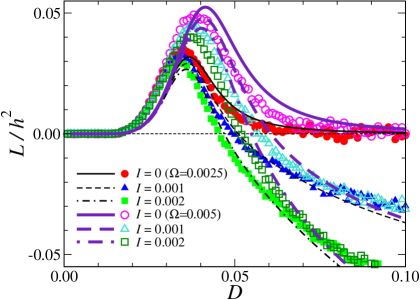
Figure 3: (Color online) Scaled MAM $L/h^{2}$ versus noise intensity $D$. The symbols and curves correspond to results of numerical simulation and the approximation Eqs. (42) and (71) for $(I,\Omega)=(0,0.0025)$ (filled circles and thin solid curve), $(0.001,0.0025)$ (filled triangles and thin dashed curve), $(0.002,0.0025)$ (filled squares and thin dashed-dotted curve), $(0,0.005)$ (open circles and thick solid curve), $(0.001,0.005)$ (open triangles and thick dashed curve) and $(0.002,0.005)$ (open squares and thick dashed-dotted curve) with $(a,b,c,d,h,\phi)=(-0.1,0.3,0.15,-0.1,0.05,0)$. The adjustable parameters in Eqs. (42) and (71) are set to $g_{L}=1.25$ and $g_{L}^{\prime}/g_{L}=0.95$ for all.

First, we give an overview of the dynamics of Eq. (1). The numerical simulation for the model was performed using the second-order stochastic Runge–Kutta method [32, 33]. To quantify the circulation of trajectory, we define the mean angular momentum (MAM):

$$L=\overline{X(t)\dot{Y}(t)-Y(t)\dot{X}(t)},$$ (6)

where $\overline{A(t)}\equiv\int_{0}^{T_{\mathrm{tot}}}\mathrm{d}t\,A(t)/T_{\mathrm{tot}}$ denotes the mean of a dynamical variable $A(t)$ over the observation time $T_{\mathrm{tot}}$ (${\gg}T_{p}$). The anticlockwise (clockwise) rotation corresponds to $L>0$ ($L<0$).

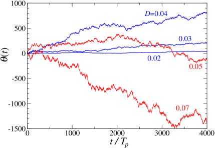
Figure 4: (Color online) Typical time series of $\theta(t)$ and its dependence on $D$. The abscissa indicates the elapsed time. The positive side of $\theta(t)$ corresponds to the anticlockwise rotation.

Figure 3 shows graphs of $L$ with respect to the noise intensity; the symbols and curves indicate the results from numerical simulations and theoretical analysis. In the numerical simulations, $\overline{A(t)}$ is obtained by averaging over 35 computational runs in addition to the long time average of $T_{\mathrm{tot}}=10^{8}$. The ratchet potential used here is that shown in Fig. 2(a), the direction of which is classified as anticlockwise (positive). Without the load, $I=0$ (open and closed circles), the MAM exhibits a bell-shaped curve with respect to $D$, which implies the magnitude of the MAM is maximized by SR. The sign of the MAM in SR depends on the ratchet direction. As the load is increased under a clockwise rotation ($I>0$), the negative region of the MAM expands. This behavior indicates that the MAM consists of a component from $H(t)\boldsymbol{N}$ and that from $\boldsymbol{f}_{I}(\boldsymbol{X})$, and these are in competition. This also implies that, for the noise intensity beyond the SR peak, the rotation forced by $\boldsymbol{f}_{I}(\boldsymbol{X})$ is more persistent for noise than that induced by the ac driving field.

Figure 4 shows a typical time series of the angular displacement defined by

$$\theta(t)=\int_{0}^{t}\mathrm{d}s\left\{\frac{X(s)\dot{Y}(s)-Y(s)\dot{X}(s)}{|\boldsymbol{X}(s)|^{2}}\right\}$$ (7)

for several noise intensities, $D\in\{0.01,0.03,0.04,0.05,0.08\}$, which is taken from the points on the curve for $(\Omega,I)=(0.005,0.002)$ in Fig. 3, where the SR peaks at $D\approx 0.04$. We see the mean angular velocity, $\overline{\dot{\theta}}=\theta(T_{\mathrm{tot}})/T_{\mathrm{tot}}$, increases and decreases with $D$ below and beyond the peak point of SR. There is also a turning point at which the rotational direction switches from anticlockwise to clockwise (see the curve for $D=0.07$).

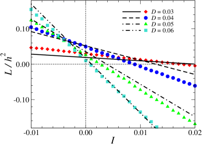
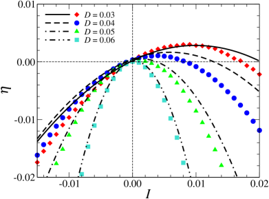
Figure 5: (Color online) $L/h^{2}$ versus load torque $I$. The symbols and curves represent numerical and theoretical results for $D=0.03$ (diamonds and solid curve), $0.04$ (circles and dashed curve), $0.05$ (triangles and dashed-dotted curve) and $0.06$ (squares and dashed-double-dotted curve) in the chiral case of Fig. 2(a) with $(\Omega,h,\phi)=(0.005,0.05,0)$.

Figure 5 shows the $I$-dependence of the MAM at several noise intensities around the SR point. We see that the sign of MAM reverses to negative values as $I$ increases. This is because the component of MAM from the load torque increases with $I$ and dominates that from the ac driving field. In addition to the above results, we should note that the MAM does not significantly depend on $\phi$. As suggested in Ref. PhysRevE.87.022144, this property can bring a robustness such that a rotary system always performs a unidirectional rotation regardless of the polarization angle.

4 Theory

We now develop a coarse-grained description of the dynamics. After introducing notation in Sect. 4.1, we obtain a master equation for coarse-grained states in Sect. 4.2, and analyze it in Sect. 4.3. In Sect. 4.4, we establish a formalism to estimate the time derivatives of energetic quantities.

4.1 Definitions

(a)	(b)

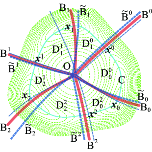
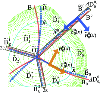
Figure 6: (Color online) (a) Definition of symbols for locally maximal and minimal points $\{\mathrm{O},\boldsymbol{x}_{\sigma}\}$, saddle points $\{\boldsymbol{x}^{\mu}\}$, ridge curves $\{\mathrm{B}_{\sigma},\mathrm{B}^{\mu}\}$ (thick solid curves), potential valley C, and domains $\{\mathrm{D}_{\sigma}^{\mu}\}$ on $V_{0}(\boldsymbol{x})$ [$(a,b,c,d)=(0.1,-0.15,0.1,-0.05)$]. Thick and thin dashed curves corresponds to the ridge curves $\{\tilde{\mathrm{B}}_{\sigma},\tilde{\mathrm{B}}^{\mu}\}$ on $V(\boldsymbol{x},t)$ [$H(t)=0.05$(thick) and $-0.05$ (thin)]. Here, $\sigma,\mu\in\{0,1,2\}$. (b) Definition of symbols for locally maximal and minimal points $\{\tilde{\mathrm{O}},\tilde{\boldsymbol{x}}_{\sigma}\}$, saddle points $\{\tilde{\boldsymbol{x}}^{\mu}\}$, ridge curves $\{\tilde{\mathrm{B}}_{\sigma},\tilde{\mathrm{B}}^{\mu}\}$ (thick dashed curves), and domains $\{\tilde{\mathrm{D}}_{\sigma}^{\mu}\}$ on $V(\boldsymbol{x},t)$ [$H(t)=0.05$]. Unit tangential and normal vectors $\{\boldsymbol{\tau}_{\sigma}^{\mu}(\boldsymbol{x}),\boldsymbol{n}_{\sigma}^{\mu}(\boldsymbol{x})\}$ or $\{\tilde{\boldsymbol{\tau}}_{\sigma}^{\mu}(\boldsymbol{x}),\tilde{\boldsymbol{n}}_{\sigma}^{\mu}(\boldsymbol{x})\}$ are defined on the boundary of $\mathrm{D}_{\sigma}^{\mu}$ or $\tilde{\mathrm{D}}_{\sigma}^{\mu}$. The vectors are the eigenvectors of the Hessian matrix $\hat{G}(\boldsymbol{x})$ on the ridge curves. The tip of the unit normal vector is directed toward the interior of the specified domain, and the associated unit tangential vector is oriented to its right. $\mathrm{B}_{\epsilon}^{\mu}$ is a domain of width $2\epsilon$ covering $\tilde{\mathrm{B}}^{\mu}$, which is indicated by a hatched region. $\Delta\mathrm{D}_{\sigma,}^{\mu}$ and $\Delta\mathrm{D}_{\sigma}^{\mu\ast}$ are the differential domain from $\mathrm{D}_{\sigma}^{\mu}$ to $\tilde{\mathrm{D}}_{\sigma}^{\mu}$.

Figure 6(a) shows our notation to describe the structure of the potential function $V_{0}(\boldsymbol{x})$. $\mathrm{C}$ denotes the potential valley. $\boldsymbol{x}_{\sigma}$ and $\boldsymbol{x}^{\mu}$ ($\sigma,\mu=0,1,2$) denote the minimal and saddle points of $V_{0}(\boldsymbol{x})$, which satisfy $\partial_{\boldsymbol{x}}V_{0}(\boldsymbol{x})=\boldsymbol{0}$. Ridge curves of $V_{0}(\boldsymbol{x})$ are denoted by $\mathrm{B}_{\sigma}$ and $\mathrm{B}^{\mu}$, where $\mathrm{B}_{\sigma}$ ($\mathrm{B}^{\mu}$) is the curve running from the origin $\mathrm{O}$ toward infinity through the minimal point $\boldsymbol{x}_{\sigma}$ (the saddle point $\boldsymbol{x}^{\mu}$). Each domain surrounded by the neighboring curves $\mathrm{B}_{\sigma}$ and $\mathrm{B}^{\mu}$ is denoted by $\mathrm{D}_{\sigma}^{\mu}$ (${\in}\{\mathrm{D}_{0}^{0},\mathrm{D}_{1}^{0},\mathrm{D}_{1}^{1},\mathrm{D}_{2}^{1},\mathrm{D}_{2}^{2},\mathrm{D}_{0}^{2}\}$).

In our coarse-grained description, the 2D space is divided into the six domains of $\mathrm{D}_{\sigma}^{\mu}$; the six events of $\boldsymbol{X}(t)\in\mathrm{D}_{\sigma}^{\mu}$ construct a state space. Although in Ref. PhysRevE.87.022144 the master equation for these six states is obtained under the static boundaries $\mathrm{B}_{\sigma}$ and $\mathrm{B}^{\mu}$, here we develop another approach based on moving ridge curves of $V(\boldsymbol{x},t)$. Then, to the notation mentioned above, we also add another notation based on $V(\boldsymbol{x},t)$; $\tilde{\boldsymbol{x}}_{\sigma}$, $\tilde{\boldsymbol{x}}^{\mu}$ ($\sigma,\mu=0,1,2$), and $\tilde{\mathrm{O}}$ denote the minimal, saddle, and maximal points of $V(\boldsymbol{x},t)$, which satisfy $\partial_{\boldsymbol{x}}V(\boldsymbol{x},t)=\boldsymbol{0}$, respectively; $\tilde{\mathrm{B}}_{\sigma}$ ($\tilde{\mathrm{B}}^{\mu}$) denotes the ridge curve of $V(\boldsymbol{x},t)$ which runs from $\tilde{\mathrm{O}}$ toward infinity through the minimal point $\tilde{\boldsymbol{x}}_{\sigma}$ (the saddle point $\tilde{\boldsymbol{x}}^{\mu}$); $\tilde{\mathrm{D}}_{\sigma}^{\mu}$ denotes a domain surrounded by the curves $\tilde{\mathrm{B}}_{\sigma}$ and $\tilde{\mathrm{B}}^{\mu}$. As shown in Fig. 6, the boundaries $\tilde{\mathrm{B}}_{\sigma}$ and $\tilde{\mathrm{B}}^{\mu}$ vary with $H(t)$.

Furthermore, we define $\boldsymbol{\tau}_{\sigma}^{\mu}(\boldsymbol{x})$ and $\boldsymbol{n}_{\sigma}^{\mu}(\boldsymbol{x})$ as unit tangential and normal vectors to the boundary of $\mathrm{D}_{\sigma}^{\mu}$ at $\boldsymbol{x}$ ($\boldsymbol{x}\in\mathrm{B}_{\sigma}$ or $\boldsymbol{x}\in\mathrm{B}^{\mu}$). Here, we orient the tip (or referential direction) of the normal vector $\boldsymbol{n}_{\sigma}^{\mu}(\boldsymbol{x})$ inside $\mathrm{D}_{\sigma}^{\mu}$, and orient the tip of the tangential vector $\boldsymbol{\tau}_{\sigma}^{\mu}(\boldsymbol{x})$ to the right-hand side (RHS) of $\boldsymbol{n}_{\sigma}^{\mu}(\boldsymbol{x})$ [Fig. 6(b)]. Similarly, corresponding to $\boldsymbol{\tau}_{\sigma}^{\mu}(\boldsymbol{x})$ and $\boldsymbol{n}_{\sigma}^{\mu}(\boldsymbol{x})$, we define the unit tangential and normal vectors $\tilde{\boldsymbol{\tau}}_{\sigma}^{\mu}(\boldsymbol{x})$ and $\tilde{\boldsymbol{n}}_{\sigma}^{\mu}(\boldsymbol{x})$ on the boundary of $\tilde{\mathrm{D}}_{\sigma}^{\mu}$, respectively.

Curvatures of the potential at $\boldsymbol{x}_{\sigma}$ and $\boldsymbol{x}^{\mu}$ are defined as follows. Near an extremum $\boldsymbol{x}_{\ast}$ (${\in}\{\boldsymbol{x}_{\sigma},\boldsymbol{x}^{\mu}\}$), we expand $V(\boldsymbol{x},t)$ as

$$V(\boldsymbol{x},t)\approx V(\boldsymbol{x}_{\ast},t)-\left\{\boldsymbol{f}_{I}(\boldsymbol{x}_{\ast})+H(t)\boldsymbol{N}\right\}\cdot\delta\boldsymbol{x}+\tfrac{1}{2}\delta\boldsymbol{x}^{{}^{\top}}\hat{G}(\boldsymbol{x}_{\ast})\delta\boldsymbol{x},$$ (8)

where $\delta\boldsymbol{x}\equiv\boldsymbol{x}-\boldsymbol{x}_{\ast}$ and $\hat{G}(\boldsymbol{x}_{\ast})\equiv\partial_{\boldsymbol{x}}\partial_{\boldsymbol{x}}^{{}^{\top}}V(\boldsymbol{x},t)\bigr{|}_{\boldsymbol{x}=\boldsymbol{x}_{\ast}}$ is the $2\times 2$ Hessian matrix at $\boldsymbol{x}_{\ast}$. We define a local coordinate system as $\boldsymbol{x}=\boldsymbol{x}_{\ast}+\xi\boldsymbol{\tau}_{\sigma}^{\mu}(\boldsymbol{x}_{\ast})+\eta\boldsymbol{n}_{\sigma}^{\mu}(\boldsymbol{x}_{\ast})$ with coordinates $(\xi,\eta)$. From the nature of ridge curves and valley, the basis vectors $\boldsymbol{\tau}_{\sigma}^{\mu}(\boldsymbol{x}_{\ast})$ and $\boldsymbol{n}_{\sigma}^{\mu}(\boldsymbol{x}_{\ast})$ satisfy

$$\hat{G}(\boldsymbol{x}_{\ast})\boldsymbol{\tau}_{\sigma}^{\mu}(\boldsymbol{x}_{\ast}) =\Lambda_{\tau}(\boldsymbol{x}_{\ast})\boldsymbol{\tau}_{\sigma}^{\mu}(\boldsymbol{x}_{\ast}),$$ (9)

$$\hat{G}(\boldsymbol{x}_{\ast})\boldsymbol{n}_{\sigma}^{\mu}(\boldsymbol{x}_{\ast}) =\Lambda_{n}(\boldsymbol{x}_{\ast})\boldsymbol{n}_{\sigma}^{\mu}(\boldsymbol{x}_{\ast}),$$ (10)

where $\Lambda_{\tau}(\boldsymbol{x}_{\ast})$ and $\Lambda_{n}(\boldsymbol{x}_{\ast})$ are the eigenvalues corresponding to $\boldsymbol{\tau}_{\sigma}^{\mu}(\boldsymbol{x}_{\ast})$ and $\boldsymbol{n}_{\sigma}^{\mu}(\boldsymbol{x}_{\ast})$, respectively. $\Lambda_{\tau}(\boldsymbol{x}_{\ast})$ and $\Lambda_{n}(\boldsymbol{x}_{\ast})$ are also the curvatures along a ridge curve and the valley. We have $\Lambda_{\tau}(\boldsymbol{x}_{\sigma})>0$ and $\Lambda_{n}(\boldsymbol{x}_{\sigma})>0$ at the minimal points, and $\Lambda_{\tau}(\boldsymbol{x}^{\mu})>0$ and $\Lambda_{n}(\boldsymbol{x}^{\mu})<0$ at the saddle points. In the local coordinate system, the third term in Eq. (8) is transformed to $\{\Lambda_{\tau}(\boldsymbol{x}_{\ast})\xi^{2}+\Lambda_{n}(\boldsymbol{x}_{\ast})\eta^{2}\}/2$.

4.2 Master equation

We denote by $P(\sigma,\mu,t)$ ($\sigma,\mu\in\{0,1,2\}$) the probability of finding the trajectory $\boldsymbol{X}(t)$ in the domain $\mathrm{D}_{\sigma}^{\mu}$ at time $t$. $P(\sigma,\mu,t)$ is related to $p(\boldsymbol{x},t)$ as

$$P(\sigma,\mu,t)\equiv\left(\delta_{\sigma,\mu}^{(3)}+\delta_{\sigma,\mu+1}^{(3)}\right)\int_{\boldsymbol{x}\in\mathrm{D}_{\sigma}^{\mu}}\mathrm{d}\boldsymbol{x}\,p(\boldsymbol{x},t),$$ (11)

where $\delta_{j,k}^{(3)}$ denotes the Kronecker delta, which is $1$ if $j=k$ and $0$ otherwise for integers $j$ and $k$, and with periodic boundary conditions $\delta_{j+3,k}^{(3)}=\delta_{j,k+3}^{(3)}=\delta_{j,k}^{(3)}$ and $\mathrm{D}_{\sigma+3}^{\mu}=\mathrm{D}_{\sigma}^{\mu+3}=\mathrm{D}_{\sigma}^{\mu}$ imposed. Hereafter, quantities with a suffixed $\sigma$ or $\mu$, such as $\boldsymbol{x}_{\sigma}$, $\boldsymbol{x}^{\mu}$, $\boldsymbol{n}_{\sigma}^{\mu}(\boldsymbol{x})$, and $\boldsymbol{\tau}_{\sigma}^{\mu}(\boldsymbol{x})$, obey these boundary conditions. The factor $\delta_{\sigma,\mu}^{(3)}+\delta_{\sigma,\mu+1}^{(3)}$ in Eq. (11) is 1 only if a specified domain $\mathrm{D}_{\sigma}^{\mu}$ is of type $\mathrm{D}_{\mu}^{\mu}$ or type $\mathrm{D}_{\mu+1}^{\mu}$. $P(\sigma,\mu,t)$ is thus nonzero only for allowed pairs of $\sigma$ and $\mu$.

Likewise, we denote by $P(\sigma,t)$ the probability of finding the trajectory $\boldsymbol{X}(t)$ in the domain $\mathrm{D}_{\sigma}^{\sigma}\cup\mathrm{D}_{\sigma}^{\sigma+2}\equiv\mathrm{D}_{\sigma}$ ($\sigma\in\{0,1,2\}$), i.e., the attractive region for $\boldsymbol{x}_{\sigma}$, and by $Q(\mu,t)$ the probability of finding $\boldsymbol{X}(t)$ in the domain $\mathrm{D}_{\mu}^{\mu}\cup\mathrm{D}_{\mu+1}^{\mu}\equiv\mathrm{D}^{\mu}$ ($\mu$ $\in$ $\{0,1,2\}$), i.e., the united domain on both sides of $\mathrm{B}^{\mu}$. Specifically,

$$P(\sigma,t) \equiv\sum_{\mu}P(\sigma,\mu,t)=\int_{\boldsymbol{x}\in\mathrm{D}_{\sigma}}\mathrm{d}\boldsymbol{x}\,p(\boldsymbol{x},t),$$ (12)

$$Q(\mu,t) \equiv\sum_{\sigma}P(\sigma,\mu,t)=\int_{\boldsymbol{x}\in\mathrm{D}^{\mu}}\mathrm{d}\boldsymbol{x}\,p(\boldsymbol{x},t).$$ (13)

Using $P(\sigma,\mu,t)$, $P(\sigma,t)$, and $Q(\mu,t)$, we define the conditional probabilities $P(\sigma\mid\mu,t)$ and $Q(\mu\mid\sigma,t)$ as

$$P(\sigma\mid\mu,t)\equiv\frac{P(\sigma,\mu,t)}{Q(\mu,t)},\quad Q(\mu\mid\sigma,t)\equiv\frac{P(\sigma,\mu,t)}{P(\sigma,t)}.$$ (14)

Now let us consider a master equation for $P(\sigma,\mu,t)$. From Eqs. (4) and (11), we have

$$\partial_{t}P(\sigma,\mu,t)=\int_{\boldsymbol{x}\in\mathrm{D}_{\sigma}^{\mu}}\mathrm{d}\boldsymbol{x}\left\{-\partial_{\boldsymbol{x}}\cdot\boldsymbol{J}(\boldsymbol{x},t)\right\}.$$ (15)

Dividing the domain of integration into $\tilde{\mathrm{D}}_{\sigma}^{\mu}$ and $\Delta\mathrm{D}_{\sigma}^{\mu}\equiv\mathrm{D}_{\sigma}^{\mu}-\tilde{\mathrm{D}}_{\sigma}^{\mu}$, we rewrite the RHS as

$$\int_{\boldsymbol{x}\in\mathrm{D}_{\sigma}^{\mu}}\mathrm{d}\boldsymbol{x}\left\{\cdot\right\}=\int_{\boldsymbol{x}\in\tilde{\mathrm{D}}_{\sigma}^{\mu}}\mathrm{d}\boldsymbol{x}\left\{\cdot\right\}+\int_{\boldsymbol{x}\in\Delta\mathrm{D}_{\sigma}^{\mu}}\mathrm{d}\boldsymbol{x}\left\{\cdot\right\},$$ (16)

where “$\,\cdot\,$” denotes $-\partial_{\boldsymbol{x}}\cdot\boldsymbol{J}(\boldsymbol{x},t)$ [${=}\partial_{t}p(\boldsymbol{x},t)$]. The difference region $\Delta\mathrm{D}_{\sigma}^{\mu}$ consists of domains $\{\boldsymbol{x}\mid\boldsymbol{x}\in\mathrm{D}_{\sigma}^{\mu},\boldsymbol{x}\notin\tilde{\mathrm{D}}_{\sigma}^{\mu}\}$ and $\{\boldsymbol{x}\mid\boldsymbol{x}\in\tilde{\mathrm{D}}_{\sigma}^{\mu},\boldsymbol{x}\notin\mathrm{D}_{\sigma}^{\mu}\}$, which we refer to as “positive” and “negative” domains, respectively. For the latter, we invert the sign of integration.

To employ Eq. (16), we assume that the noise intensity $D$ is much smaller than the potential difference $\Delta V$ ($\Delta V/D\gg 1$) and that $h$, $\Omega$, and $I$ are very small. These assumptions are often used in studies of SR[30, 31]. In this situation, the probability density of $\boldsymbol{X}(t)$ is localized at the minima of $V(\boldsymbol{x},t)$ and can be regarded as near thermal equilibrium around them. We thus assume that thermal equilibrium for the PDF, $\boldsymbol{J}(\boldsymbol{x},t)=\boldsymbol{0}$, approximately holds along the curve $\tilde{\mathrm{B}}_{\sigma}$. Applying this to the first term in Eq. (16), we have

$$\int_{\boldsymbol{x}\in\tilde{\mathrm{D}}_{\sigma}^{\mu}}\mathrm{d}\boldsymbol{x}\left\{-\partial_{\boldsymbol{x}}\cdot\boldsymbol{J}(\boldsymbol{x},t)\right\} \approx\int_{\boldsymbol{x}\in\tilde{\mathrm{B}}^{\mu}}\mathrm{d}\boldsymbol{x}\,\tilde{\boldsymbol{n}}_{\sigma}^{\mu}(\boldsymbol{x})\cdot\boldsymbol{J}(\boldsymbol{x},t)$$

$$\equiv\left(\delta_{\sigma,\mu+1}^{(3)}-\delta_{\sigma,\mu}^{(3)}\right)J^{\mu}(t),$$ (17)

where $J^{\mu}(t)$ is the probability current, i.e., the transition rate, from $\tilde{\mathrm{D}}_{\mu}^{\mu}$ to $\tilde{\mathrm{D}}_{\mu+1}^{\mu}$ induced by thermal activation and is positive for anticlockwise rotations. Note that $\tilde{\mathrm{B}}^{\mu}$ lies on the moving potential barrier. It is reasonable to expect that the magnitude of $\boldsymbol{J}(\boldsymbol{x},t)$ reflects the degree of deviation from thermal equilibrium and to assume that $|\boldsymbol{J}(\boldsymbol{x},t)|$ is locally maximal (minimal) at $\tilde{\boldsymbol{x}}^{\mu}$ ($\tilde{\boldsymbol{x}}_{\sigma}$), and that $|\boldsymbol{J}(\boldsymbol{x},t)|$ increases as $\boldsymbol{x}$ nears the boundary $\tilde{\mathrm{B}}^{\mu}$ along the valley. Thus, $\tilde{\mathrm{B}}^{\mu}$ can be taken as a natural boundary between states. Indeed, the current density may have an $O(I)$ bias due to the load force such that $\boldsymbol{J}(\boldsymbol{x},t)\sim O(I)$ everywhere, although it is assumed to vanish along $\tilde{\mathrm{B}}_{\sigma}$. We expect that this bias would smoothly vanish as $I\rightarrow 0$ and only contribute a meaningful effect to states near thermal equilibrium. This bias is integrated into $J^{\mu}(t)$ at the boundary $\tilde{\mathrm{B}}^{\mu}$.

Because $h$ is small and $\Delta V/D\gg 1$, the PDF nearly vanishes around the origin O and the temporal maximum $\tilde{\mathrm{O}}$. We can thus regard both O and $\tilde{\mathrm{O}}$ as essentially being the same point and all the curves $\mathrm{B}_{\sigma}$, $\tilde{\mathrm{B}}_{\sigma}$, $\mathrm{B}^{\mu}$, and $\tilde{\mathrm{B}}^{\mu}$ as starting at O. This allows us to consider the difference domain $\Delta\mathrm{D}_{\sigma}^{\mu}$ as being composed of one domain surrounded by $\mathrm{B}_{\sigma}$ and $\tilde{\mathrm{B}}_{\sigma}$ and another surrounded by $\mathrm{B}^{\mu}$ and $\tilde{\mathrm{B}}^{\mu}$, denoted $\Delta\mathrm{D}_{\sigma\ast}^{\mu}$ and $\Delta\mathrm{D}_{\sigma}^{\mu\ast}$, respectively. With $\Delta\mathrm{D}_{\sigma}^{\mu}$ separated into $\Delta\mathrm{D}_{\sigma\ast}^{\mu}$ and $\Delta\mathrm{D}_{\sigma}^{\mu\ast}$, the second term in Eq. (16) reads

$$\int_{\Delta\mathrm{D}_{\sigma}^{\mu}}\mathrm{d}\boldsymbol{x}\left\{\cdot\right\}=\int_{\Delta\mathrm{D}_{\sigma}^{\mu\ast}}\mathrm{d}\boldsymbol{x}\left\{\cdot\right\}+\int_{\Delta\mathrm{D}_{\sigma\ast}^{\mu}}\mathrm{d}\boldsymbol{x}\left\{\cdot\right\}.$$ (18)

Using the notation $\partial_{t}P(\sigma,\mu,t)\bigr{|}_{Q}\equiv-\int_{\Delta\mathrm{D}_{\sigma}^{\mu\ast}}\mathrm{d}\boldsymbol{x}\left\{\cdot\right\}$ and $\partial_{t}P(\sigma,\mu,t)\bigr{|}_{P}\equiv\int_{\Delta\mathrm{D}_{\sigma\ast}^{\mu}}\mathrm{d}\boldsymbol{x}\left\{\cdot\right\}$, from Eqs. (16)–(18) we express Eq. (15) as

$$\partial_{t}P(\sigma,\mu,t)\approx \left(\delta_{\sigma,\mu+1}^{(3)}-\delta_{\sigma,\mu}^{(3)}\right)J^{\mu}(t)$$

$$-\partial_{t}P(\sigma,\mu,t)\bigr{|}_{Q}+\partial_{t}P(\sigma,\mu,t)\bigr{|}_{P}.$$ (19)

Under the assumptions $O(h)\ll\Delta V$ and $\Omega T_{r}\ll 1$, the displacement and velocity of the movement of the boundaries, $\tilde{\mathrm{B}}_{\sigma}$ and $\tilde{\mathrm{B}}^{\mu}$, can be regarded as sufficiently small and sufficiently slow, respectively, in the following arguments. In this case, we consider the roles of the current $J^{\mu}(t)$ and the two following terms in Eq. (19) individually, by applying virtual variations of the boundaries under certain conditions. For $J^{\mu}(t)$, when there is no boundary variation, i.e., $\tilde{\mathrm{B}}_{\sigma}=\mathrm{B}_{\sigma}$ and $\tilde{\mathrm{B}}^{\mu}=\mathrm{B}^{\mu}$, we can ignore the last two terms in Eq. (19) and thus have $\partial_{t}P(\sigma,t)\approx J^{\sigma-1}(t)-J^{\sigma}(t)$ and $\partial_{t}Q(\mu,t)\approx 0$. This implies that the time evolution of $P(\sigma,t)$ is dominated by $J^{\mu}(t)$, or the action of $J^{\mu}(t)$ is connected to the time evolution of $P(\sigma,t)$.

For $\partial_{t}P(\sigma,\mu,t)\bigr{|}_{Q}$ and $\partial_{t}P(\sigma,\mu,t)\bigr{|}_{P}$, we consider variation of $\tilde{\mathrm{B}}^{\mu}$ (or $\tilde{\mathrm{B}}_{\sigma}$) under the conditions that the other boundaries are fixed to their reference states $\mathrm{B}_{\sigma^{\prime}}$ and $\mathrm{B}^{\mu^{\prime}}$ ($\sigma^{\prime}\neq\sigma$, $\mu^{\prime}\neq\mu$) at $H(t)=0$, and that $J^{\mu^{\prime}}(t)=0$ for $\mu^{\prime}\in\{\mu-1,\mu+1\}$ (or $\mu^{\prime}\in\{\sigma-1,\sigma,\sigma+1\}$). Under these conditions, the influence from the other boundaries being ignored, we can identify an effect only of the specified variation of boundary, and clarify the respective roles of $\partial_{t}P(\mu,\mu,t)\bigr{|}_{Q}$ and $\partial_{t}P(\mu,\mu,t)\bigr{|}_{P}$ as follows. For simplicity, considering only the case of $\sigma=\mu$ in $\partial_{t}P(\sigma,\mu,t)\bigr{|}_{Q}$ and $\partial_{t}P(\sigma,\mu,t)\bigr{|}_{P}$ we have

$$\partial_{t}P(\mu,\mu,t)\bigr{|}_{Q} =\int_{\boldsymbol{x}\in\tilde{\mathrm{B}}^{\mu}}\,\mathrm{d}\boldsymbol{x}\,\tilde{\boldsymbol{n}}_{\mu}^{\mu}(\boldsymbol{x})\cdot\boldsymbol{J}(\boldsymbol{x},t)-\int_{\boldsymbol{x}\in\mathrm{B}^{\mu}}\,\mathrm{d}\boldsymbol{x}\,\boldsymbol{n}_{\mu}^{\mu}(\boldsymbol{x})\cdot\boldsymbol{J}(\boldsymbol{x},t)$$

$$\approx\int_{\boldsymbol{x}\in\mathrm{B}^{\mu}}\,\mathrm{d}\boldsymbol{x}\,\boldsymbol{n}_{\mu}^{\mu}(\boldsymbol{x})\cdot\left\{\boldsymbol{J}(\tilde{\boldsymbol{x}}(\boldsymbol{x}),t)-\boldsymbol{J}(\boldsymbol{x},t)\right\},$$ (20)

$$\partial_{t}P(\mu,\mu,t)\bigr{|}_{P} \approx\int_{\boldsymbol{x}\in\mathrm{B}_{\mu}}\,\mathrm{d}\boldsymbol{x}\,\boldsymbol{n}_{\mu}^{\mu}(\boldsymbol{x})\cdot\boldsymbol{J}(\boldsymbol{x},t),$$ (21)

where $\tilde{\boldsymbol{x}}=\tilde{\boldsymbol{x}}(\boldsymbol{x})$ is a mapping from $\boldsymbol{x}$ on $\mathrm{B}^{\mu}$ to its nearest point, $\tilde{\boldsymbol{x}}$, on $\tilde{\mathrm{B}}^{\mu}$ and the approximation $\boldsymbol{n}_{\sigma}^{\mu}(\boldsymbol{x})\approx\tilde{\boldsymbol{n}}_{\sigma}^{\mu}(\tilde{\boldsymbol{x}}(\boldsymbol{x}))$ is applied (the boundaries $\tilde{\mathrm{B}}^{\mu}$ and $\mathrm{B}^{\mu}$ [$\tilde{\mathrm{B}}_{\mu}$ and $\mathrm{B}_{\mu}$] are assumed to be sufficiently close). We can regard $\partial_{t}P(\mu,\mu,t)\bigr{|}_{Q}$ [$\partial_{t}P(\mu,\mu,t)\bigr{|}_{P}$] as a relative current to $J^{\mu}(t)$ because each RHS of Eqs. (20) and (21) represents the integral of the flux through $\tilde{\mathrm{B}}^{\mu}$ ($\mathrm{B}_{\mu}$) relative to that through $\mathrm{B}^{\mu}$ ($\tilde{\mathrm{B}}_{\mu}$), where $\boldsymbol{J}(\boldsymbol{x},t)=\boldsymbol{0}$ on $\tilde{\mathrm{B}}_{\mu}$ in Eq. (21). In Eq. (20), since we have assumed that the current attains a local maximum on $\tilde{\mathrm{B}}^{\mu}$ because $|\boldsymbol{J}(\tilde{\boldsymbol{x}}(\boldsymbol{x}),t)\cdot\boldsymbol{n}_{\mu}^{\mu}(\boldsymbol{x})|\geq|\boldsymbol{J}(\boldsymbol{x},t)\cdot\boldsymbol{n}_{\mu}^{\mu}(\boldsymbol{x})|$, we have that $\partial_{t}P(\mu,\mu,t)\bigr{|}_{Q}$ represents the incoming relative current into the domain $\mathrm{D}_{\mu}^{\mu}$. From the virtual variation of $\tilde{\mathrm{B}}^{\mu}$, by ignoring the current into the domain $\mathrm{D}^{\mu}$, we regard $Q(\mu,t)$ as a constant in Eq. (20). Then, using the conditional probability in Eq. (14), we have

$$\int_{\boldsymbol{x}\in\mathrm{B}^{\mu}}\mathrm{d}\boldsymbol{x}\,\frac{\boldsymbol{n}_{\mu}^{\mu}(\boldsymbol{x})\cdot\left\{\boldsymbol{J}(\boldsymbol{x},t)-\boldsymbol{J}(\tilde{\boldsymbol{x}}(\boldsymbol{x}),t)\right\}}{Q(\mu,t)}=\partial_{t}P(\mu\mid\mu,t)$$ (22)

and $\partial_{t}P(\mu,\mu,t)\bigr{|}_{Q}=Q(\mu,t)\partial_{t}P(\mu\mid\mu,t)$. Similarly, by applying such a virtual variation to $\tilde{\mathrm{B}}_{\mu}$ in Eq. (21), and ignoring the current into the domain $\mathrm{D}_{\mu}$, we regard $P(\mu,t)$ as a constant and have $\partial_{t}P(\mu,\mu,t)\bigr{|}_{P}=P(\mu,t)\partial_{t}Q(\mu\mid\mu,t)$.

As a result of the above approximation and simplification, Eq. (19) reads

$$\partial_{t}P(\sigma,\mu,t)\approx\left(\delta_{\sigma,\mu+1}^{(3)}-\delta_{\sigma,\mu}^{(3)}\right)J^{\mu}(t)+J_{\sigma}^{\mu}(t),$$ (23)

$$J_{\sigma}^{\mu}(t)\equiv\left(\delta_{\sigma,\mu+1}^{(3)}+\delta_{\sigma,\mu}^{(3)}\right)\left\{P(\sigma,t)\partial_{t}Q(\mu\mid\sigma,t)-Q(\mu,t)\partial_{t}P(\sigma\mid\mu,t)\right\}.$$ (24)

Because, as mentioned above, we are treating the currents in Eq. (19) separately, the total current in Eq. (23) can be read as a superposition of currents that cause independent actions; the current $J^{\mu}(t)$ is relevant only to the evolution of $P(\sigma,t)$ without affecting $Q(\mu\mid\sigma,t)$, whereas the two (relative) currents in $J_{\sigma}^{\mu}(t)$ are related to the change in the ratios of $P(\sigma,\mu,t)$ to $P(\sigma,t)$ and to $Q(\mu,t)$. In Sect. 4.4, we shall see $J_{\sigma}^{\mu}(t)$ is indispensable in explaining the circulation induced by the ac driving field.

To complete the master equation, we have to express $J^{\mu}(t)$ with known quantities. With this, we can approximately solve Eqs. (23) and (24) by regarding $J_{\sigma}^{\mu}(t)$ as a small quantity, which, as shown below, enters at the level of $O(h^{2})$. We first analyze the linearized master equation,

$$\partial_{t}P(\sigma,\mu,t)\approx\delta_{\sigma,\mu+1}^{(3)}J^{\mu}(t)-\delta_{\sigma,\mu}^{(3)}J^{\mu}(t),$$ (25)

within a linear response treatment in Sect. 4.3, in which $P(\sigma,t)$ and $J^{\mu}(t)$ are related to the driving field.

4.3 Linear response treatment

By applying reaction rate theory [34] or Langer’s method [35] for $J^{\mu}(t)$ in Eq. (17), we obtain

$$J^{\mu}(t)\approx W(\mu,\mu,t)P(\mu,t)-W(\mu+1,\mu,t)P(\mu+1,t),$$ (26)

$$W(\sigma,\mu,t)\equiv\frac{1}{2\pi}e^{-\{V(\boldsymbol{x}^{\mu},t)-V(\boldsymbol{x}_{\sigma},t)\}/D}\sqrt{\frac{H_{\tau}H_{n}|G_{n}|}{G_{\tau}}},$$ (27)

where $W(\mu+1,\mu,t)$ [$W(\mu,\mu,t)$] is the transition rate from the state $\boldsymbol{X}(t)\in\mathrm{D}_{\mu+1}$ to the state $\boldsymbol{X}(t)\in\mathrm{D}_{\mu}^{\mu}$ [from $\boldsymbol{X}(t)\in\mathrm{D}_{\mu}$ to $\boldsymbol{X}(t)\in\mathrm{D}_{\mu+1}^{\mu}$] [Note1]Supplemental material for the derivation of Eqs. (26)–(29) is provided online.. $H_{\tau}$ and $H_{n}$ ($G_{n}$ and $G_{\tau}$) are the eigenvalues of the Hessian matrix, as defined in Eqs. (9) and (10), at the potential minimum (saddle), for which we have $H_{\tau}\equiv\Lambda_{\tau}(\boldsymbol{x}_{\sigma})$ and $H_{n}\equiv\Lambda_{n}(\boldsymbol{x}_{\sigma})$ [$G_{n}\equiv\Lambda_{n}(\boldsymbol{x}^{\mu})<0$ and $G_{\tau}\equiv\Lambda_{\tau}(\boldsymbol{x}^{\mu})$] from the threefold symmetry. Also, we obtain the relationship between $P(\sigma,\mu,t)$ and $Q(\mu\mid\sigma,t)$ in Eq. (14) as

$$P(\sigma,\mu,t)\approx\left(\delta_{\sigma,\mu}^{(3)}+\delta_{\sigma+2,\mu}^{(3)}\right)Q(\mu\mid\sigma,t)P(\sigma,t),$$ (28)

$$Q(\mu\mid\sigma,t)\approx\frac{1}{2}\left\{1+\frac{2\boldsymbol{f}_{\sigma}\cdot\boldsymbol{n}_{\sigma}^{\mu}(\boldsymbol{x}_{\sigma})}{\sqrt{2\pi DH_{n}}}\right\},$$ (29)

where $\boldsymbol{f}_{\sigma}\equiv\boldsymbol{f}_{I}(\boldsymbol{x}_{\sigma})+H(t)\boldsymbol{N}$. This derivation is based on the condition of local thermal equilibrium around the potential minima [36].

To obtain the relationships of $P(\sigma,t)$, $Q(\mu,t)$, and $J^{\mu}(t)$ to the driving fields in $O(h)$ and $O(I)$, we expand $P(\sigma,t)$ and $W(\sigma,\mu,t)$ in Eqs. (26) and (27) as

$$P(\sigma,t)\approx P_{0}(\sigma)+P_{1}(\sigma,t),$$ (30)

$$W(\sigma,\mu,t)\approx W_{0}\left\{1+\frac{H(t)}{D}\boldsymbol{N}\cdot(\boldsymbol{x}^{\mu}-\boldsymbol{x}_{\sigma})-\frac{V_{I}(\boldsymbol{x}^{\mu})-V_{I}(\boldsymbol{x}_{\sigma})}{D}\right\},$$ (31)

where the first and the second [and the third in Eq. (31)] terms are of zeroth- and first-order in $h$ and $I$, respectively, we assume $\sum_{\sigma}P_{0}(\sigma)=1$ and $\sum_{\sigma}P_{1}(\sigma,t)=0$ for the normalization, and the transition rate

$$W_{0}\equiv\frac{1}{2\pi}e^{-\{V_{0}(\boldsymbol{x}^{0})-V_{0}(\boldsymbol{x}_{0})\}/D}\sqrt{\frac{H_{\tau}H_{n}|G_{n}|}{G_{\tau}}}$$ (32)

results from the thermal activation without load and ac driving fields. Here we neglect the $I$- and $h$-dependence in $H_{\tau}$, $H_{n}$, $G_{\tau}$, and $G_{n}$ for simplification, i.e., in which we replace $\hat{G}(\boldsymbol{x}_{\ast})$ in Eqs. (9) and (10) with $\partial_{\boldsymbol{x}}\partial_{\boldsymbol{x}}^{{}^{\top}}V_{0}(\boldsymbol{x})\bigr{|}_{\boldsymbol{x}=\boldsymbol{x}_{\ast}}$. Note that we have used the threefold symmetry in $V_{0}(\boldsymbol{x})$, e.g., $V_{0}(\boldsymbol{x}_{\sigma})=V_{0}(\boldsymbol{x}_{\sigma+1})$, for $W_{0}$.

Substituting Eqs. (30) and (31) into Eq. (26), the zeroth-order equality of $J^{\mu}(t)=0$ reads $P_{0}(\sigma)=1/3$, and, up to $O(h)$ and $O(I)$, $J^{\mu}(t)$ reads

$$J^{\mu}(t)\approx W_{0}\biggl{\{} P_{1}(\mu,t)-P_{1}(\mu+1,t)+\frac{H(t)}{3D}\boldsymbol{N}\cdot\left(\boldsymbol{x}_{\mu+1}-\boldsymbol{x}_{\mu}\right)$$

$$+\frac{V_{I}(\boldsymbol{x}_{\mu})-V_{I}(\boldsymbol{x}_{\mu+1})}{3D}\biggr{\}}.$$ (33)

Applying this to $\partial_{t}P(\sigma,t)\approx J^{\sigma-1}(t)-J^{\sigma}(t)$ from Eq. (25), we find $P_{1}(\sigma,t)\approx(h\boldsymbol{N}\cdot\boldsymbol{x}_{\sigma}/3)\operatorname{Re}\left[\tilde{\chi}(\Omega)e^{i\Omega t}\right]$ with $\tilde{\chi}(\Omega)=3W_{0}/\{D(i\Omega+3W_{0})\}$[28]. Note that we have $\boldsymbol{x}_{\sigma+1}+\boldsymbol{x}_{\sigma-1}=-\boldsymbol{x}_{\sigma}$ and $V_{I}(\boldsymbol{x}_{\mu+1})-V_{I}(\boldsymbol{x}_{\mu})=I/3$ from the threefold symmetry.

Thus, up to $O(h)$, we obtain $P(\sigma,t)$ as

$$P(\sigma,t) \approx\frac{1}{3}\left\{1+h\frac{\boldsymbol{N}\cdot\boldsymbol{x}_{\sigma}}{D}\operatorname{Re}\left[\frac{3W_{0}e^{i\Omega t}}{i\Omega+3W_{0}}\right]\right\}.$$ (34)

Also, substituting Eqs. (29) and (34) into $Q(\mu,t)=\sum_{\sigma\in\{\mu,\mu+1\}}Q(\mu\mid\sigma,t)P(\sigma,t)$, we get

$$Q(\mu,t)\approx\frac{1}{3}\biggl{\{} 1+\frac{H(t)\boldsymbol{N}\cdot\left(\boldsymbol{n}_{\mu}^{\mu}-\boldsymbol{n}_{\mu+1}^{\mu+1}\right)}{\sqrt{2\pi DH_{n}}}$$

$$\quad+\frac{h}{2D}\boldsymbol{N}\cdot\left(\boldsymbol{x}_{\mu}+\boldsymbol{x}_{\mu+1}\right)\operatorname{Re}\left[\frac{3W_{0}e^{i\Omega t}}{i\Omega+3W_{0}}\right]\biggr{\}},$$ (35)

where $\boldsymbol{n}_{\mu}^{\mu}(\boldsymbol{x}_{\mu})\equiv\boldsymbol{n}_{\mu}^{\mu}$, $\boldsymbol{n}_{\mu+1}^{\mu}(\boldsymbol{x}_{\mu+1})=-\boldsymbol{n}_{\mu+1}^{\mu+1}$, and we have used $\boldsymbol{f}_{I}(\boldsymbol{x}_{\mu})\cdot\boldsymbol{n}_{\mu}^{\mu}=\boldsymbol{f}_{I}(\boldsymbol{x}_{\mu+1})\cdot\boldsymbol{n}_{\mu+1}^{\mu+1}$ from the threefold symmetry. From Eqs. (34) and (33), we find

$$J^{\mu}(t)\approx\frac{hW_{0}}{3D}\boldsymbol{N}\cdot(\boldsymbol{x}_{\mu+1}-\boldsymbol{x}_{\mu})\operatorname{Re}\left[\frac{i\Omega e^{i\Omega t}}{i\Omega+3W_{0}}\right]-\frac{W_{0}I}{9D},$$ (36)

where the first and second terms are the respective currents driven by $H(t)$ and the load.

4.4 Coarse-grained kinetics

We next develop a method to estimate kinetic quantities in terms of a coarse-grained description. For a comparable argument in the case of 1D ratchet models, see Ref. JPSJ.66.1234. The expectation value for the time derivative of a quantity $A\{\boldsymbol{X}(t)\}\equiv A$ reads

$$\langle\dot{A}\rangle =\int\mathrm{d}\boldsymbol{x}\,\partial_{\boldsymbol{x}}A\cdot\boldsymbol{J}\quad[\boldsymbol{J}\equiv\boldsymbol{J}(\boldsymbol{x},t)]$$

$$=\sum_{\mu}\int_{\tilde{\mathrm{D}}^{\mu}_{\mu}\cup\tilde{\mathrm{D}}^{\mu}_{\mu+1}}\mathrm{d}\boldsymbol{x}\,\partial_{\boldsymbol{x}}A\cdot\boldsymbol{J}+\sum_{\sigma,\mu}\int_{\Delta\mathrm{D}^{\mu}_{\sigma}}\mathrm{d}\boldsymbol{x}\,\partial_{\boldsymbol{x}}A\cdot\boldsymbol{J}$$

$$\approx\sum_{\mu}\Delta A^{\mu}J^{\mu}(t)+\sum_{\sigma,\mu}\Delta A_{\sigma}^{\mu}J_{\sigma}^{\mu}(t),$$ (37)

with the two types of current as in Eqs. (23) and (24). Assuming that $\boldsymbol{J}$ lies along the potential valley (see Sect. 4.2), for example, the integral over $\Delta\mathrm{D}^{\mu\ast}_{\mu}$ [see Eqs. (18)–(21)] in the second term in the second line can be approximated as

$$\int_{\Delta\mathrm{D}^{\mu\ast}_{\mu}} \mathrm{d}\boldsymbol{x}\,\partial_{\boldsymbol{x}}A\cdot\boldsymbol{J}$$

$$\approx-\int_{\boldsymbol{x}\in\mathrm{C}}\mathrm{d}\boldsymbol{x}\left(\partial_{\boldsymbol{x}}A\right)_{\mathrm{C}}\int_{\boldsymbol{x}\in\mathrm{B}^{\mu}}\mathrm{d}\boldsymbol{x}\,\boldsymbol{n}_{\mu}^{\mu}(\boldsymbol{x})\cdot\left\{\boldsymbol{J}(\tilde{\boldsymbol{x}}(\boldsymbol{x}),t)-\boldsymbol{J}(\boldsymbol{x},t)\right\},$$ (38)

where $\mathrm{C}$ denotes the curve along the valley in the related domain and $(\partial_{\boldsymbol{x}}A)_{\mathrm{C}}$ the tangential derivative along the curve. In other words, each double integral over the 2D domain is converted into repeated integrals over $\mathrm{C}$ and its orthogonal curves nearly parallel to $\mathrm{B}^{\mu}$ (or $\mathrm{B}_{\sigma}$ for $\Delta\mathrm{D}^{\mu}_{\sigma\ast}$) and then decoupled into independent integrals as in Eq. (38). A similar procedure is applied to the other integrals in Eq. (37). Thus, we regard $\Delta A^{\mu}$ as a representative difference of $A$ between the domains $\mathrm{D}^{\mu}_{\mu+1}$ and $\mathrm{D}^{\mu}_{\mu}$ and $\Delta A_{\sigma}^{\mu}$ as that between the boundaries $\mathrm{B}_{\sigma}$ and $\mathrm{B}^{\mu}$ of $\mathrm{D}^{\mu}_{\sigma}$.

Recall here the currents $J^{\mu}(t)$, $-Q(\mu,t)\partial_{t}P(\mu\mid\mu,t)$, $P(\mu,t)\partial_{t}Q(\mu\mid\mu,t)$, $Q(\mu,t)\partial_{t}P(\mu+1\mid\mu,t)$, and $-P(\mu+1,t)\partial_{t}Q(\mu\mid\mu+1,t)$ (anticlockwise), which increase and decrease $A$ on the downstream and upstream sides, respectively, on the specified boundary. For each of these currents, there is a possible coupling with one of the characteristic differences $A(\boldsymbol{x}_{\mu+1})-A(\boldsymbol{x}_{\mu})$, $A(\boldsymbol{x}_{\mu+1})-A(\boldsymbol{x}^{\mu})$, and $A(\boldsymbol{x}^{\mu})-A(\boldsymbol{x}_{\mu})$ as $\Delta A^{\mu}$ or $\Delta A_{\sigma}^{\mu}$ in Eq. (37). Each product of a current and the characteristic difference represents transport of $A$ through the specified boundary. In Eq. (37), $\langle\dot{A}\rangle$ is expressed as a superposition of such transports. However, there are no clear definitions for the relationships between $\Delta A^{\mu}$ ($\Delta A_{\sigma}^{\mu}$) and the characteristic difference. We therefore determine these empirically by comparison with the results of numerical simulations.

For instance, by applying Eq. (37) to the velocity we obtain

$$\langle\dot{\boldsymbol{X}}(t)\rangle \approx g_{V}\sum_{\mu}(\boldsymbol{x}_{\mu+1}-\boldsymbol{x}_{\mu})J^{\mu}(t)+g_{V}^{\prime}\sum_{\sigma,\mu}(\boldsymbol{x}^{\mu}-\boldsymbol{x}_{\sigma})\left(\delta_{\sigma,\mu}^{(3)}+\delta_{\sigma,\mu+1}^{(3)}\right)$$

$$\quad\times\left\{P(\sigma,t)\partial_{t}Q(\mu\mid\sigma,t)-Q(\mu,t)\partial_{t}P(\sigma\mid\mu,t)\right\}.$$ (39)

In the first term, $\boldsymbol{x}_{\mu+1}-\boldsymbol{x}_{\mu}$ gives the representative difference in the position vector between $\mathrm{D}^{\mu}_{\mu+1}$ and $\mathrm{D}^{\mu}_{\mu}$. In the second term, with $\sigma$ set to equal $\mu$ in the summation, $(\boldsymbol{x}^{\mu}-\boldsymbol{x}_{\mu})P(\mu,t)\partial_{t}Q(\mu\mid\mu,t)$ and $(\boldsymbol{x}_{\mu}-\boldsymbol{x}^{\mu})Q(\mu,t)\partial_{t}P(\mu\mid\mu,t)$ give the components of the velocity caused by variations in $\tilde{\mathrm{B}}_{\mu}$ and $\tilde{\mathrm{B}}^{\mu}$, respectively. We use the adjustable parameters $g_{V}$ and $g_{V}^{\prime}$ to absorb errors arising from the approximation in Eq. (37) and determine these by fits to the data. Such adjustable parameters, introduced here and below, are dimensionless, and we regard them as $O(1)$.

For the expectation value for the MAM in Eq. (6), assuming $L\approx\langle L\rangle$ for sufficiently large $T_{\mathrm{tot}}$, we have $L=L^{(I)}+L^{(h)}$ with

$$L^{(I)} \approx\frac{g_{L}}{2}\sum_{\mu}\left\{\boldsymbol{x}^{\mu}\times(\boldsymbol{x}_{\mu+1}-\boldsymbol{x}_{\mu})\right\}_{z}\overline{J^{\mu}(t)},$$ (40)

$$L^{(h)} \approx g_{L}^{\prime}\sum_{\sigma,\mu}(\boldsymbol{x}_{\sigma}\times\boldsymbol{x}^{\mu})_{z}\left(\delta_{\sigma,\mu}^{(3)}+\delta_{\sigma,\mu+1}^{(3)}\right)$$

$$\quad\times\overline{\left\{P(\sigma,t)\partial_{t}Q(\mu\mid\sigma,t)-Q(\mu,t)\partial_{t}P(\sigma\mid\mu,t)\right\}},$$ (41)

where $L^{(I)}$ and $L^{(h)}$ come from the two types of current. Each summand in Eq. (40) represents the $z$-component of the angular momentum at $\boldsymbol{x}^{\mu}$, i.e., the vector product between $\boldsymbol{x}^{\mu}$ and $(\boldsymbol{x}_{\mu+1}-\boldsymbol{x}_{\mu})J^{\mu}(t)/2$, where the latter is the mean of $(\boldsymbol{x}_{\mu+1}-\boldsymbol{x}^{\mu})J^{\mu}(t)$ and $(\boldsymbol{x}^{\mu}-\boldsymbol{x}_{\mu})J^{\mu}(t)$.

Applying Eqs. (34)–(36) to Eqs. (40)–(41), we obtain

$$L^{(I)}\approx-\frac{g_{L}W_{0}I}{6D}\{(\boldsymbol{x}_{0}-\boldsymbol{x}_{1})\times\boldsymbol{x}^{0}\}_{z}$$ (42)

and $L^{(h)}$ as in Eq. (71) in Appendix A. Note that because of the threefold symmetry, $\{(\boldsymbol{x}_{\mu+1}-\boldsymbol{x}_{\mu})\times\boldsymbol{x}^{\mu}\}_{z}$ is independent of $\mu$. Using Eqs. (42) and (71), we rewrite $L$ as

$$L\approx\frac{g_{L}W_{0}}{6D}\{(\boldsymbol{x}_{0}-\boldsymbol{x}_{1})\times\boldsymbol{x}^{0}\}_{z}\,\{I_{0}(D)-I\},$$ (43)

$$I_{0}(D)\equiv-\frac{9g_{L}^{\prime}h^{2}\Omega^{2}}{2g_{L}\sqrt{2\pi DH_{n}}}\frac{\boldsymbol{x}_{0}\cdot\boldsymbol{n}_{0}^{0}}{\Omega^{2}+(3W_{0})^{2}}.$$ (44)

For the mirror image of the potential, the sign of $\left\{(\boldsymbol{x}_{0}-\boldsymbol{x}_{1})\times\boldsymbol{x}^{0}\right\}_{z}$ is inverted, but $\boldsymbol{x}_{0}\cdot\boldsymbol{n}_{0}^{0}$ remains unchanged. One can check that $\left\{(\boldsymbol{x}_{0}-\boldsymbol{x}_{1})\times\boldsymbol{x}^{0}\right\}_{z}\geq 0$ for a positive ratchet potential: When $I=I_{0}(D)$, the load balances the ac-induced torque. The expression for $I_{0}(D)$ in Eq. (44) implies that a stronger torque from the ac driving field to cope with a load requires the ratchet potential to have a greater asymmetry with respect to $\boldsymbol{x}_{0}\cdot\boldsymbol{n}_{0}^{0}$, because of the latter’s relation to the degree of asymmetry.[28] $I_{0}(D)$ indicates the minimal load strength or coercive (load) torque, which is taken from the coercive field—in magnetic terminology—and the load torque for $I>I_{0}(D)$ overwhelms the ac-induced torque.

The curves in Fig. 3 refer to plots of Eq. (43); they qualitatively agree with the numerical results. The adjustable parameters are set to $g_{L}=1.25$ and $g_{L}^{\prime}/g_{L}=0.95$ throughout this paper. The peak of the curves with respect $D$ identifies SR and mainly comes from the factor $W_{0}\Omega^{2}/\{\Omega^{2}+(3W_{0})^{2}\}$ in Eq. (71), which has a maximum for $\Omega=3W_{0}$.

In Fig. 5, the value of $I$ at $L=0$ tends to increase as $D$ decreases. This is explained by Eq. (44), because $I_{0}(D)$ is a monotonically decreasing function of $D$. This implies that for a stronger coercive load torque, SR should occur in a smaller $D$-region to gain the advantage, because the coercive torque increases as the peak point for SR ($\Omega\approx 3W_{0}$) shifts to small-$D$ regions. We describe a related implication of the $D^{-1/2}$ factor on $I_{0}(D)$ in Sect. 6.2.

5 Energetics

We consider the energetics and the efficiency[37, 38, 39, 40] in the force conversion from the linearly polarized ac field to the torque for the load. Our approach follows the methods developed in Refs. PhysRevLett.83.903,PhysRevE.68.021906,PhysRevE.70.061105, and adds two dimensional characteristics to them. We separate the slowly varying part $\boldsymbol{V}$ from $\dot{\boldsymbol{X}}$ as $\dot{\boldsymbol{X}}\equiv\boldsymbol{V}+\delta\dot{\boldsymbol{X}}$, where $\delta\dot{\boldsymbol{X}}$ denotes the fluctuating part whereas $\boldsymbol{V}$ has a long-term correlation with the driving field. Furthermore, $\boldsymbol{V}$ is decomposed as $\boldsymbol{V}\equiv\langle\dot{\boldsymbol{X}}\rangle+\boldsymbol{V}_{\theta}$, where $\langle\dot{\boldsymbol{X}}\rangle$ is regarded as a translational mode, which is in fact an oscillation in the direction along the driving field $H(t)\boldsymbol{N}$ [See the argument below Eq. (84)], and $\boldsymbol{V}_{\theta}$ represents a steady rotational mode around the origin. For simplicity, we approximate $\langle\dot{\boldsymbol{X}}\rangle$ as $\langle\dot{\boldsymbol{X}}\rangle\approx\operatorname{Re}[\tilde{\boldsymbol{V}}_{h}e^{i\Omega t}]$ with the Fourier coefficient $\tilde{\boldsymbol{V}}_{h}=(2/T_{p})\int_{0}^{T_{p}}\mathrm{d}t\langle\dot{\boldsymbol{X}}(t)\rangle e^{-i\Omega t}$, of the fundamental harmonic (or the linear response part).

For the energetics on the rotational mode, the force $\boldsymbol{F}=-\partial_{\boldsymbol{X}}V(\boldsymbol{X},t)$ is also decomposed as

$$\boldsymbol{F}\equiv\gamma\langle\dot{\boldsymbol{X}}\rangle+\tilde{\boldsymbol{F}},$$ (45)

where $\gamma\langle\dot{\boldsymbol{X}}\rangle=\langle\boldsymbol{F}\rangle$ is the mean frictional force, and $\tilde{\boldsymbol{F}}$ involves the force relevant to the rotational mode. This corresponds to the decomposition $\dot{\boldsymbol{X}}\equiv\langle\dot{\boldsymbol{X}}\rangle+\tilde{\dot{\boldsymbol{X}}}$. With the component $\tilde{\dot{\boldsymbol{X}}}$, which is unbiased from the translational mode and leaves the rotational mode, we define relative angular momentum and angular velocity as

$$L^{\prime}(t) \equiv X(\dot{Y}-\langle\dot{Y}\rangle)-Y(\dot{X}-\langle\dot{X}\rangle),$$ (46)

$$\omega^{\prime}(t) \equiv\frac{X(\dot{Y}-\langle\dot{Y}\rangle)-Y(\dot{X}-\langle\dot{X}\rangle)}{X^{2}+Y^{2}}.$$ (47)

Now, let us consider the energy (power) balance equation (EBE). The derivation of EBE involves calculating the long time average of the inner product of Eq. (1) and $\boldsymbol{F}$, i.e., $\gamma\overline{\dot{\boldsymbol{X}}\cdot\boldsymbol{F}}=\overline{\left|\boldsymbol{F}\right|^{2}}+\overline{\boldsymbol{F}\cdot\boldsymbol{R}}$; details are given in Appendix B, which contains the decomposition of $\overline{\left|\boldsymbol{F}\right|^{2}}$ to terms relevant to the two modes and the estimation of $\overline{\boldsymbol{F}\cdot\boldsymbol{R}}$. We thus find the EBE as

$$\overline{\dot{\boldsymbol{X}}\cdot\boldsymbol{f}_{h}}=\overline{(-\dot{\boldsymbol{X}}\cdot\boldsymbol{f}_{I})}+\gamma\left(\overline{|\langle\dot{\boldsymbol{X}}\rangle|^{2}}+\overline{L^{\prime}}\overline{\omega^{\prime}}\right)+Q_{T},$$ (48)

where $\boldsymbol{F}=\boldsymbol{f}_{h}+\boldsymbol{f}_{I}$ [$\boldsymbol{f}_{h}\equiv H(t)\boldsymbol{N}$, $\boldsymbol{f}_{I}\equiv\boldsymbol{f}_{I}(\boldsymbol{X}(t))$], and

$$\gamma Q_{T}\equiv \;k_{\mathrm{B}}T(\overline{\partial_{x}F_{x}+\partial_{y}F_{y}})+\overline{\left(\frac{X\tilde{F}_{x}+Y\tilde{F}_{y}}{\sqrt{X^{2}+Y^{2}}}\right)^{2}}$$

$$+\gamma^{2}\overline{\left\{\gamma^{-1}(X\tilde{F}_{y}-Y\tilde{F}_{x})-\overline{L^{\prime}}\right\}\left(\frac{1}{\gamma}\frac{X\tilde{F}_{y}-Y\tilde{F}_{x}}{X^{2}+Y^{2}}-\overline{\omega^{\prime}}\right)}\,.$$ (49)

The left-hand side (LHS) in Eq. (48) represents the input power of the driving field $\boldsymbol{f}_{h}$ into the rotary system, and is denoted by $P_{h}\equiv\overline{\dot{\boldsymbol{X}}\cdot\boldsymbol{N}H(t)}$. The first term on the RHS represents an output power of the system for the load:

$$P_{I}\equiv-\overline{\dot{\boldsymbol{X}}\cdot\boldsymbol{f}_{I}(\boldsymbol{X})}=\overline{\dot{V}_{I}(\boldsymbol{X})}=\frac{I}{2\pi}\overline{\dot{\theta}(t)}.$$ (50)

The second term on the RHS, $P_{d}\equiv\gamma\left(\overline{|\langle\dot{\boldsymbol{X}}\rangle|^{2}}+\overline{L^{\prime}}\overline{\omega^{\prime}}\right)$, represents the energy dissipation rate of the two modes (Supposing the rotor drags and rotates the surrounding molecules, this power is spent to retain such a movement). However, we replace it with

$$P_{d}\approx\frac{\gamma}{2}|\tilde{\boldsymbol{V}}_{h}|^{2}+\gamma L\overline{\dot{\theta}}$$ (51)

for simplicity. Here, as shown in Eqs. (82) and (83) in Appendix B, the difference between $\overline{L^{\prime}}$ and $L$ (also that between $\overline{\omega^{\prime}}$ and $\overline{\dot{\theta}}$) can be regarded as $o(h^{2})$. The last term, $Q_{T}$, in Eq. (48) represents the power of the thermally activated fluctuations. In particular, the second term in Eq. (49) is the mean of the squared radial component of $\tilde{\boldsymbol{F}}$, which excludes the two modes, and the third is the covariance of $L^{\prime}(t)$ and $\omega^{\prime}(t)$. The latter involves that the relationship between $L^{\prime}(t)$ and $\omega^{\prime}(t)$ is not constant but fluctuates. Thus, the last two terms in Eq. (49) represent the fluctuation increased by additional degree of freedom to the rotational orbit.

Here, we consider two types of output/input power ratio, $\rho$ and $\eta$:

$$\rho=\frac{P_{d}+P_{I}}{P_{h}},$$ (52)

$$\eta=\frac{P_{d}^{\prime}+P_{I}}{P_{h}},\quad P_{d}^{\prime}\equiv\gamma L\overline{\dot{\theta}},$$ (53)

where $\rho$ denotes the ratio of the total output power of the slowly varying component to the input power, and characterizes the preservation of the powers of motion in the time scale ${\sim}\Omega^{-1}$, and $\eta$ denotes the power conversion efficiency of the ac driving field to the rotational motion subject to a load. In the latter, $P_{d}$ is replaced with $P_{d}^{\prime}$, so that the numerator of $\eta$ consists of only the output powers of the rotational mode. This corresponds to the so-called rectification efficiency (or generalized efficiency) in the 1D ratchet models in Refs. PhysRevE.68.021906,PhysRevLett.83.903,PhysRevE.70.061105,PhysRevE.75.061115. An advantage of the generalized efficiency is that it gives nonvanishing values even in the absence of loads. Below, we show both numerical simulation and approximation results for the above-mentioned powers, $\rho$ and $\eta$.

(a)	(b)

Figure 7: (Color online) (a) Scaled output power $P_{I}/h^{2}$ versus $D$. (b) $P_{I}/h^{2}$ versus $I$. The graph settings are the same as those in Fig. 3 [panel (a)] and Fig. 5 [panel (b)], respectively. The curves indicate Eq. (56), which adjustable parameters are set to $g_{O}=0.47g_{L}$ and $g_{O}^{\prime}/g_{O}=g_{L}^{\prime}/g_{L}=0.95$.

First, let us consider the expectation value for $P_{I}$ in Eq. (50). Hereafter, we assume that $P_{I}=\langle P_{I}\rangle$ with the ergodic hypothesis and that the other powers obey this. In a similar way to $L$ in Sect. 4.4, partitioning $P_{I}$ into $P_{I}^{(I)}$ and $P_{I}^{(h)}$ ($P_{I}=P_{I}^{(I)}+P_{I}^{(h)}$) related to the currents $J^{\mu}(t)$ and $J_{\sigma}^{\mu}(t)$, we obtain the following estimates:

$$P_{I}^{(I)}\approx \;g_{O}\sum_{\mu}\{V_{I}(\boldsymbol{x}_{\mu+1})-V_{I}(\boldsymbol{x}_{\mu})\}\overline{J^{\mu}(t)},$$ (54)

$$P_{I}^{(h)}\approx \;g_{O}^{\prime}\sum_{\sigma,\mu}\left\{V_{I}(\boldsymbol{x}_{\mu+1})-V_{I}(\boldsymbol{x}_{\mu})\right\}\left(\delta_{\sigma,\mu}^{(3)}-\delta_{\sigma,\mu+1}^{(3)}\right)$$

$$\times\overline{\left\{P(\sigma,t)\partial_{t}Q(\mu\mid\sigma,t)-Q(\mu,t)\partial_{t}P(\sigma\mid\mu,t)\right\}},$$ (55)

where $g_{O}$ and $g_{O}^{\prime}$ are adjustable parameters. In Eq. (54), each summand represents the rate of energy change for the transition $\boldsymbol{x}_{\mu}\rightarrow\boldsymbol{x}_{\mu+1}$ due to thermal activation. From Eq. (36), we get $P_{I}^{(I)}\approx-g_{O}W_{0}I^{2}/(9D)$. In Eq. (55), each summand represents the energy consumption for the movement in the direction $\boldsymbol{x}_{\mu}\rightarrow\boldsymbol{x}_{\mu+1}$ induced by the deformation of $\tilde{\mathrm{D}}_{\mu}^{\mu}$ and $\tilde{\mathrm{D}}_{\mu+1}^{\mu}$.

Using Eq. (72) in Appendix A, we obtain

$$P_{I} \approx\frac{g_{O}W_{0}I}{9D}\left\{I_{0}(D)-I\right\},$$ (56)

where $I_{0}(D)$ is given in Eq. (44), and $g_{O}^{\prime}/g_{O}=g_{L}^{\prime}/g_{L}$ is assumed so that $P_{I}$ is proportional to $L$ for $I_{0}(D)\geq I$. Figure 7 shows graphs of $P_{I}$ with respect to (a) $D$ and (b) $I$. In panel (b), $P_{I}$ is approximately parabolic taking positive values for $0<I<I_{0}(D)$ with a maximum at $I=I_{0}(D)/2$. The maximum output power is estimated as $g_{O}W_{0}\{I_{0}(D)\}^{2}/(36D)$.

Figure 8: (Color online) Scaled input power $P_{h}/h^{2}$ versus $D$. The graph settings are the same as those in Fig. 3. The curves indicate Eq. (57), which adjustable parameter is set at $g_{V}=0.75$ throughout this paper.

Next, we estimate the expectation value for $P_{h}$. From Eqs. (36) and (39), keeping terms up to $O(h^{2})$, we obtain

$$P_{h} \approx g_{V}\sum_{\mu}\left\{(\boldsymbol{x}_{\mu+1}-\boldsymbol{x}_{\mu})\cdot\boldsymbol{N}\right\}\overline{H(t)J^{\mu}(t)}$$

$$=\frac{g_{V}h^{2}}{6D}\frac{W_{0}\Omega^{2}}{\Omega^{2}+(3W_{0})^{2}}\sum_{\mu}\left\{(\boldsymbol{x}_{\mu+1}-\boldsymbol{x}_{\mu})\cdot\boldsymbol{N}\right\}^{2}$$

$$=\frac{3g_{V}h^{2}|\boldsymbol{x}_{0}|^{2}}{4D}\frac{W_{0}\Omega^{2}}{\Omega^{2}+(3W_{0})^{2}},$$ (57)

where, between the second and third lines, we have used Eq. (69) in Appendix A and $\sum_{\mu}\left\{(\boldsymbol{x}_{\mu+1}-\boldsymbol{x}_{\mu})\cdot\boldsymbol{N}\right\}^{2}=9|\boldsymbol{x}_{0}|^{2}/2$ [See Eqs. (74) and (75)]. Setting $g_{V}=0.75$, Fig. 8 shows graphs of $P_{h}$ with respect to $D$. The peak for $P_{h}$ is due to SR. $P_{h}$ has no strong dependence on $I$ and $\phi$.

(a)	(b)

Figure 9: (Color online) Energy dissipation rates of (a) the slowly varying modes $P_{d}$ and (b) the rotational mode $P_{d}^{\prime}$ versus $D$. The graph settings are the same as those in Fig. 3. The curves indicate Eqs. (59) [panel (a)] and (60) [panel (b)].

(a)	(b)

Figure 10: (Color online) (a) Power ratio $\rho$ and (b) efficiency $\eta$ versus $D$. The graph settings are the same as those in Fig. 3. The curves indicate Eqs. (62) [panel (a)] and $\eta$ made of Eqs. (53), (56), (57) and (60) [panel (b)]. In panel (a), the $I$-dependence of the curves is slight.

For $\tilde{\boldsymbol{V}}_{h}$, using the first term in Eq. (39) for the $O(h)$ approximation, we have

$$\tilde{\boldsymbol{V}}_{h}\approx\frac{g_{V}hW_{0}}{3D}\frac{i\Omega}{i\Omega+3W_{0}}\sum_{\mu}\left\{(\boldsymbol{x}_{\mu+1}-\boldsymbol{x}_{\mu})\cdot\boldsymbol{N}\right\}(\boldsymbol{x}_{\mu+1}-\boldsymbol{x}_{\mu}).$$ (58)

Substituting this and Eq. (56) into Eq. (51), we obtain

$$P_{d}\approx\frac{9g_{V}^{2}\gamma h^{2}\left|\boldsymbol{x}_{0}\right|^{4}}{8D^{2}}\frac{\Omega^{2}W_{0}^{2}}{\Omega^{2}+(3W_{0})^{2}}+P_{d}^{\prime},$$ (59)

$$P_{d}^{\prime}\approx\frac{\pi g_{L}g_{O}\gamma W_{0}^{2}}{27D^{2}}\{(\boldsymbol{x}_{0}-\boldsymbol{x}_{1})\times\boldsymbol{x}^{0}\}_{z}\left\{I_{0}(D)-I\right\}^{2},$$ (60)

where, in the calculation of $|\tilde{\boldsymbol{V}}_{h}|^{2}$, we have used

$$\biggl{|}\sum_{\mu}\{(\boldsymbol{x}_{\mu+1}-\boldsymbol{x}_{\mu})\cdot\boldsymbol{N}\}(\boldsymbol{x}_{\mu+1}-\boldsymbol{x}_{\mu})\biggr{|}^{2}=\frac{3^{4}}{4}|\boldsymbol{x}_{0}|^{4},$$ (61)

which is obtained in terms of Eqs. (74) and (75) in Appendix A by noting that the vector in $|\cdots|$ on the LHS is collinear with $\boldsymbol{N}$.

Figure 9(a) shows graphs of $P_{d}$ with respect to $D$. We see the curve is similar to that of $P_{h}$, because the first term in Eq. (51) is the dominant contribution. Figure 9(b) shows graphs of $P_{d}^{\prime}$ with respect to $D$. The maximum and minimum of the curve correspond to the SR peak and the zero point where $I=I_{0}(D)$, respectively. $P_{d}$ and $P_{d}^{\prime}$ are quantities in $O(h^{2})$ and $O(h^{4})$, and $P_{d}^{\prime}$ is much smaller than $P_{d}$. Although, Eq. (59) well agrees with the numerical result, the minimum point of Eq. (60) somewhat differs from the numerical result. This deviation is believed to stem from the several approximations made, in particular, in estimating the transition rate with the saddle point approximation and neglecting the $I$-dependence in the curvatures (the Hessian matrix).

(a)	(b)

Figure 11: (Color online) (a) $\rho$ and (b) $\eta$ versus $I$. The graph settings are the same as those in Fig. 5.

From Eqs. (57) and (59), we obtain $\rho$ and $\eta$ as

$$\rho=\eta+\frac{3g_{V}\gamma\left|\boldsymbol{x}_{0}\right|^{2}}{2D}W_{0},$$ (62)

where $\eta$ is determined from Eqs. (56), (57), and (60). Figure 10 shows graphs of $\rho$ and $\eta$ with respect to $D$. The behavior around $D=0$ in Fig. 10(a), in which $\rho$ quickly drops from $\rho=1$, is due to a minor oscillation caused by the ac field around a potential minimum that is irrelevant to the unidirectional rotation and must be excluded from consideration. $P_{d}$ is dominated by the energy dissipation of the translational mode, and $P_{d}$ adds a much larger contribution to the numerator in $\rho$ than $P_{I}$. In contrast to $\rho$, $\eta$ in Fig. 10(b) involves the characteristic points of SR and $I=I_{0}(D)$. Although $\eta$ is very small, we believe it will become larger if we improve the potential shape.

Figure 11 shows graphs of $\rho$ and $\eta$ with respect to $I$. $\rho$ and $\eta$ are positive for a finite range of $I$, although not all the range is displayed. For small $|I|$, the analytical results agree relatively well with the numerical results except for their magnitudes. The deviation may be large depending on $D$ and the setting of the adjustable parameters.

6 Discussion

6.1 Relationship between $P_{I}$ and $L$

Figure 12: (Color online) Relationship between $P_{I}$ and $L$. The symbols and curves indicate the numerical and the theoretical results for $I=0$ (filled circles, thick solid curve), $0.001$ (filled triangles, thick dashed curve), $0.002$ (filled squares, thick dashed-dotted curve), $0.005$ (filled diamonds, thin solid curve), $0.01$ (open circles, dotted curve) and $0.02$ (open triangles, dashed-double-dotted curve) at $(a,b,c,d,h,\Omega,\phi)=(-0.1,0.3,0.15,-0.1,0.05,0.005,0)$.

In the strongly dissipative system, in which inertia is neglected as Eq. (1), the MAM is proportional to the (mean) viscous torque, i.e., $\gamma L$ ($\gamma=1$), cf. terminal velocity in viscous media. From Eq. (43), for $I_{0}(D)>I$, the viscous torque is an excessive product of the applied ac field. Both $L$ and $P_{I}$ depend on the angular velocity, and the two quantities are expected to be connected in a simple relation. Here, in terms of these quantities, let us discuss another characteristic of the motor other than the efficiencies. Figure 12 shows the relationship between $P_{I}$ and $L$ through parameter $D$. We see that $L$ is a single-valued function of $P_{I}$. Furthermore, although $L$ is a nonlinear function of $P_{I}$ on the whole, we can approximate them as being proportional within the first quadrant. Indeed, the hypothetical expressions for $L$ in Eqs. (40) and (41) and those for $P_{I}$ in Eqs. (54) and (55) are arranged so as to be proportional. Consequently, from Eqs. (43) and (56), we have

$$L=\frac{3g_{L}}{2g_{O}I}\{(\boldsymbol{x}_{0}-\boldsymbol{x}_{1})\times\boldsymbol{x}^{0}\}_{z}P_{I}.$$ (63)

From $P_{I}=I/(2\pi)\,\overline{\dot{\theta}(t)}$, we can regard $\left\{(\boldsymbol{x}_{0}-\boldsymbol{x}_{1})\times\boldsymbol{x}^{0}\right\}_{z}$ as a moment of inertia.

For synthetic or natural molecular motor systems, if it is possible to experimentally measure the MAM (viscous torque) and the angular velocity $\overline{\dot{\theta}(t)}$ for a sufficiently wide range of temperature under conditions of constant load, we may obtain results comparable to the graph in Fig. 12, although the obtained result may not necessarily obey Eq. (63). On the measurement of torque of biological molecular motors, in Ref. PhysRevLett.104.218103, a method based on the fluctuation theorem[45, 46] and the Jarzynski equality[47] is proposed.

6.2 $D^{-3/2}$ scaling of SR peaks as a characteristic of 2D ratchet systems

$S=1.25$	$S=1.50$
$S=1.75$	$S=2.00$

Figure 13: (Color online) Contour graphs of $V_{0}(\boldsymbol{x})$ parameterized as $(a,b,c,d)=(-0.1S,0.3S,0.15S^{2},-0.1S)$ with $S\in\{1.25,1.50,1.75,2.00\}$. For $S=1.00$, see Fig. 2(a). The settings is the same as in Fig. 2(a).

(a)	(b)

Figure 14: (Color online) (a) Scaled MAM and (b) mean angular velocity $\omega/\Omega$ versus $D$ for a series of potentials parameterized by $S$ as $(a,b,c,d)=(-0.1S,0.3S,0.15S^{2},-0.1S)$. The symbols indicate the results of numerical simulations for $S=1.00$ (diamonds), $1.25$ (downward-pointing triangles), $1.50$ (squares), $1.75$ (circles), and $2.00$ (upward-pointing triangles). The other parameters are $(I,h,\Omega,\phi)=(0,0.05,0.0025,0)$. The axes of the main and inset plots are on log–log and linear scales. The additional curves represent (a) $L=C_{L}D^{-\alpha}$ with $(C_{L},\alpha)=(0.00136,1)$ (dashed curve), $(0.00022,1.5)$ (solid curve), and $(0.000062,2)$ (dotted curve) and (b) $\omega/\Omega=C_{\omega}D^{-\alpha}$ with $(C_{\omega},\alpha)=(0.00136,1)$ (dashed curve), $(0.00026,1.5)$ (solid curve), and $(0.000066,2)$ (dotted curve).

The factor of $D^{-1/2}$ in the expression for $I_{0}(D)$ in Eq. (44) stems from the current $J_{\sigma}^{\mu}(t)$, which is caused by the deformation of the state boundaries. The factor can be regarded as a characteristic of 2D ratchet systems driven by external fields, because it arises from the first term in Eq. (68), which involves the basic property in two dimensions that the driving field will not always lie along the rotational direction (or the potential valley), i.e., $\boldsymbol{N}\cdot(\boldsymbol{n}_{\mu+1}^{\mu+1}-\boldsymbol{n}_{\mu}^{\mu})$. (We exclude the possibility of cases with such tight coupling that the directions of the driving force and the motion are always parallel, which may be more appropriately described as 1D ratchet systems.) Here we present evidence of the $D^{-1/2}$ dependence with numerical simulations for the MAM and the mean angular velocity $\omega\equiv\overline{\dot{\theta}}=2\pi P_{I}/I$ at $I=0$. Consider a trace of SR peaks in a series of potentials parameterized as $(a,b,c,d)=(-0.1S,0.3S,0.15S^{2},-0.1S)$ by $S\in\{1.00,1.25,1.50,1.75,2.00\}$, which are shown in Figs. 2(a) and 13. This parameterization makes the contour plots similar (compare the shapes of the potential valleys) but controls the potential differences, with $\Delta V\approx 0.209$ ($S=1.00$), $0.285$ ($1.25$), $0.358$ ($1.50$), $0.423$ ($1.75$), and $0.479$ ($2.00$). As mentioned at the end of Sect. 4.4, the SR peak lies near the point of $D$ that satisfies $\Omega=3W_{0}$ for $I=0$. The peak position, $D_{\mathrm{SR}}$, increases with $\Delta V$, i.e., $D_{\mathrm{SR}}\approx C_{D}\Delta V$, from the logarithm of $\Omega=3W_{0}$ and Eq. (32), where $C_{D}$ may also depend on $\Delta V$ through the curvature of the potential. From Eq. (43) or Eq. (71), the peak height depends on $D$ as $L\approx C_{L}D_{\mathrm{SR}}^{-3/2}$, where $C_{L}$ involves geometric information about the potential, i.e., $C_{L}\propto\left\{(\boldsymbol{x}_{0}-\boldsymbol{x}_{1})\times\boldsymbol{x}^{0}\right\}_{z}\boldsymbol{x}_{0}\cdot\boldsymbol{n}_{0}^{0}/\sqrt{H_{n}}$. Similarly, from Eq. (72), the SR peak of $\omega$ has a form $\omega/\Omega\approx C_{\omega}D_{\mathrm{SR}}^{-3/2}$ with $C_{\omega}\propto\boldsymbol{x}_{0}\cdot\boldsymbol{n}_{0}^{0}/\sqrt{H_{n}}$.

One can thus see the $D_{\mathrm{SR}}^{-3/2}$ scaling for the peaks in the plot of $L$ or $\omega$ for $D$ as a manifestation of the factor of $D^{-1/2}$ in the expression for $I_{0}(D)$, within a range of $S$ such that the factor $C_{L}$ (or $C_{\omega}$) does not significantly change. Figure 14 shows $L/h^{2}$ and $\omega/\Omega$ as a function of $D$ for the series of potentials. In the additional curves (for $C_{L}D^{-\alpha}$ and $C_{\omega}D^{-\alpha}$, $\alpha\in\{1,1.5,2\}$), for which the values of $C_{L}$ and $C_{\omega}$ were determined by eye, it can be seen that the $D^{-3/2}$ curve is the closest to a tangent to the envelopes of the peaks. This result is consistent with the above argument. Deviations here between the curve and envelope may be caused by the dependence of $C_{L}$ or $C_{\omega}$ on the details of the shape of the potential. Also note that this scaling does not hold when $\Delta V$ is so small that SR is replaced by another behavior.

7 Summary

An artificial molecular rotary system driven by linearly polarized ac fields, which can generate a unidirectional rotation under a load, was studied using the three-tooth Brownian rotary ratchet model. The dynamics are described by the Langevin equation for a particle in the 2D three-tooth ratchet potential with threefold symmetry. To consider how much load for which the ac induced torque can bear a positive work (coercive load torque), and how to estimate efficiency in the power conversion from the ac-field input to the output under the load, we have developed an approach treating them with coarse-grained variables.

As a part of our coarse-grained kinetic description, we have proposed a master equation which is extended by incorporating the dynamical effects from oscillating boundaries between states. Here, the oscillation is assumed to be sufficiently small and slow. In addition to the normal current over the potential barrier under thermal activation, the master equation involves a current induced by moving boundaries (the ridge curves), which is applied to explain the circulation induced by the driving force. This also enables us to estimate expectation values for the time derivative of physical quantities. Using this, we have obtained approximate expressions for the MAM and the powers composing the energy balance equation. From the MAM result, we have obtained the coercive torque against the torque induced by the ac driving field with $I_{0}(D)$ given in Eq. (44). The factor $D^{-1/2}$ in $I_{0}(D)$ is associated with the feature of the driving field that is not always along the trajectory of the motion, and can be regarded as a characteristic of 2D ratchet systems possessing such driving forces. The coercive torque is also relevant to the maximum output power for the load as $P_{I}\propto W_{0}\{I_{0}(D)\}^{2}/D$ at $I=I_{0}(D)/2$. We have also suggested the determination of the linear relationship between the MAM and angular velocity for another characterization of the molecular motor.

We have characterized the energetics with the two types of output/input power ratio; the numerator of $\rho$ is the output power of the slowly varying component of the motion, that of $\eta$ is the output power of the rotational mode, and their denominator is the input power of the driving field. Because only the rotational mode produces useful work for the load, $\eta$ measures the efficiency in the force conversion to the torque. In the present design of the potential, the linear response part (the translational mode) dominated the slowly varying components, and provided the main contribution to the energy dissipation rate for the viscous resistance. Accordingly, $\rho$ was dominated by the energy dissipation, and the magnitude of $\eta$ was small. However, our main purpose in this paper was not to demonstrate models of larger $\eta$, but to construct an analytical framework for the performance estimation of 2D ratchet models. In fact, our approach has incorporated several 2D properties into the kinetic description in Sect. 4.4 and the EBE [Eq. (48) and, especially, $Q_{T}$ in Eq. (49)].

For a larger efficiency, we consider that the ratio between the translational and rotational modes depends on the potential structure, and we can increase the relative magnitude of the rotational mode by making the best use of the ratchet effect. Designing such models that can demonstrate an efficient force conversion may be an underlying theme of research on molecular motor systems. A possible approach is to make the potential shape much harder for motions other than rotational motion, because the presented potential may be too soft for radial motion, and to improve the potential design to increase $I_{0}(D)$ optimizing relevant geometrical factors. Although we have not deeply investigated how the fluctuation $Q_{T}$ influences the efficiency, that may also bring important information for the design, especially if an analytic expression for $Q_{T}$ is obtained. These remain problems for future study.

Appendix A AC Induced Angular Momentum $L^{(h)}$ and Output Power $P_{I}^{(h)}$

Using Eqs. (14) and (25), the second line of Eq. (41) or (55) is found to be

$$\overline{P(\sigma,t)\partial_{t}Q(\mu\mid\sigma,t)-Q(\mu,t)\partial_{t}P(\sigma\mid\mu,t)}$$

$$\quad\approx\left(\delta_{\sigma,\mu+1}^{(3)}-\delta_{\sigma,\mu}^{(3)}\right)\overline{\ln\frac{P(\sigma,t)}{Q(\mu,t)}J^{\mu}(t)}.$$ (64)

Substituting this into $L^{(h)}$ and $P_{I}^{(h)}$ in Eqs. (41) and (55), we find

$$L^{(h)}\approx g_{L}^{\prime}\sum_{\mu}\left\{(\boldsymbol{x}_{\mu+1}\times\boldsymbol{x}^{\mu})_{z}\>\overline{\ln\frac{P(\mu+1,t)}{Q(\mu,t)}J^{\mu}(t)}-(\boldsymbol{x}_{\mu}\times\boldsymbol{x}^{\mu})_{z}\,\overline{\ln\frac{P(\mu,t)}{Q(\mu,t)}J^{\mu}(t)}\right\},$$ (65)

$$P_{I}^{(h)}\approx g_{O}^{\prime}\sum_{\mu}\left\{V_{I}(\boldsymbol{x}_{\mu})-V_{I}(\boldsymbol{x}_{\mu+1})\right\}\overline{\left\{\ln\frac{P(\mu+1,t)}{Q(\mu,t)}+\ln\frac{P(\mu,t)}{Q(\mu,t)}\right\}J^{\mu}(t)}\,.$$ (66)

Let us estimate $L^{(h)}$ and $P_{I}^{(h)}$ within $O(h^{2})$ and $O(Ih^{2})$, respectively. First, using Eqs. (34) and (35), we expand $\ln\{P(\sigma,t)/Q(\mu,t)\}$ in $h$ as

$$\ln\frac{P(\sigma,t)}{Q(\mu,t)}\approx \;\frac{H(t)}{\sqrt{2\pi DH_{n}}}\boldsymbol{N}\cdot\left(\boldsymbol{n}_{\mu+1}^{\mu+1}-\boldsymbol{n}_{\mu}^{\mu}\right)$$

$$+\frac{h}{2D}\boldsymbol{N}\cdot(2\boldsymbol{x}_{\sigma}-\boldsymbol{x}_{\mu}-\boldsymbol{x}_{\mu+1})\operatorname{Re}\left[\frac{3W_{0}}{i\Omega+3W_{0}}e^{i\Omega t}\right].$$ (67)

Using this multiplied by $J^{\mu}(t)$, we have

$$\overline{\ln\frac{P(\sigma,t)}{Q(\mu,t)}J^{\mu}(t)}\approx \;\frac{1}{\sqrt{2\pi DH_{n}}}\boldsymbol{N}\cdot\left(\boldsymbol{n}_{\mu+1}^{\mu+1}-\boldsymbol{n}_{\mu}^{\mu}\right)\overline{H(t)J^{\mu}(t)}$$

$$+\frac{h}{2D}\boldsymbol{N}\cdot(2\boldsymbol{x}_{\sigma}-\boldsymbol{x}_{\mu}-\boldsymbol{x}_{\mu+1})\;\overline{\operatorname{Re}\left[\frac{3W_{0}e^{i\Omega t}}{i\Omega+3W_{0}}\right]J^{\mu}(t)}\,.$$ (68)

From Eq. (36), we estimate $\overline{H(t)J^{\mu}(t)}\equiv K_{1}$ and $\overline{\operatorname{Re}\left[3W_{0}e^{i\Omega t}/(i\Omega+3W_{0})\right]J^{\mu}(t)}\equiv K_{2}$ as

$$K_{1} \approx\frac{hW_{0}}{3D}\boldsymbol{N}\cdot(\boldsymbol{x}_{\mu+1}-\boldsymbol{x}_{\mu})\overline{H(t)\operatorname{Re}\left[\frac{i\Omega}{i\Omega+3W_{0}}e^{i\Omega t}\right]}$$

$$=\frac{h^{2}}{6D}\frac{W_{0}\Omega^{2}}{\Omega^{2}+(3W_{0})^{2}}\boldsymbol{N}\cdot(\boldsymbol{x}_{\mu+1}-\boldsymbol{x}_{\mu}),$$ (69)

$$K_{2} \approx\frac{hW_{0}}{3D}\boldsymbol{N}\cdot(\boldsymbol{x}_{\mu+1}-\boldsymbol{x}_{\mu})\overline{\;\operatorname{Re}\left[\frac{3W_{0}e^{i\Omega t}}{i\Omega+3W_{0}}\right]\operatorname{Re}\left[\frac{i\Omega e^{i\Omega t}}{i\Omega+3W_{0}}\right]}$$

$$=0.$$ (70)

Applying Eqs. (68)–(70) to Eqs. (65) and (66), we get

$$L^{(h)} \approx\frac{g_{L}^{\prime}}{\sqrt{2\pi DH_{n}}}\sum_{\mu}\boldsymbol{N}\cdot\left(\boldsymbol{n}_{\mu+1}^{\mu+1}-\boldsymbol{n}_{\mu}^{\mu}\right)\{(\boldsymbol{x}_{\mu+1}-\boldsymbol{x}_{\mu})\times\boldsymbol{x}^{\mu}\}_{z}K_{1}$$

$$=-\frac{3g_{L}^{\prime}h^{2}}{4D\sqrt{2\pi DH_{n}}}\frac{W_{0}\Omega^{2}}{\Omega^{2}+(3W_{0})^{2}}\left\{(\boldsymbol{x}_{0}-\boldsymbol{x}_{1})\times\boldsymbol{x}^{0}\right\}_{z}\boldsymbol{x}_{0}\cdot\boldsymbol{n}_{0}^{0}\,,$$ (71)

$$P_{I}^{(h)} \approx-\frac{g_{O}^{\prime}h^{2}I}{2D\sqrt{2\pi DH_{n}}}\frac{W_{0}\Omega^{2}}{\Omega^{2}+(3W_{0})^{2}}\boldsymbol{x}_{0}\cdot\boldsymbol{n}_{0}^{0}\,.$$ (72)

Here, in addition to the symmetric property, we have used

$$\sum_{\mu}\left\{\boldsymbol{N}\cdot(\boldsymbol{n}_{\mu+1}^{\mu+1}-\boldsymbol{n}_{\mu}^{\mu})\right\}\left\{\boldsymbol{N}\cdot(\boldsymbol{x}_{\mu+1}-\boldsymbol{x}_{\mu})\right\}=\frac{9}{2}\boldsymbol{x}_{0}\cdot\boldsymbol{n}_{0}^{0}\,.$$ (73)

Combining Eq. (72) with Eq. (44), we obtain the first term in Eq. (56).

Equation (73) is obtained as follows. Rewriting $\boldsymbol{x}_{\mu}$ and $\boldsymbol{n}_{\mu}^{\mu}$ as

$$\boldsymbol{x}_{\mu} =|\boldsymbol{x}_{0}|\begin{pmatrix}\cos(2\pi\mu/3+\alpha)\\ \sin(2\pi\mu/3+\alpha)\end{pmatrix},\quad\boldsymbol{n}_{\mu}^{\mu}=\begin{pmatrix}\cos(2\pi\mu/3+\beta)\\ \sin(2\pi\mu/3+\beta)\end{pmatrix}$$ (74)

with the constants $\alpha$ and $\beta$ independent of $\mu$, we have

$$\boldsymbol{N}\cdot(\boldsymbol{x}_{\mu+1}-\boldsymbol{x}_{\mu})=\sqrt{3}\,|\boldsymbol{x}_{0}|\sin\left(\phi-\alpha-\frac{2\pi}{3}\mu-\frac{\pi}{3}\right),$$ (75)

and $\boldsymbol{N}\cdot(\boldsymbol{n}_{\mu+1}^{\mu+1}-\boldsymbol{n}_{\mu}^{\mu})$ as that of Eq. (75) with the replacements $\alpha\rightarrow\beta$ and $|\boldsymbol{x}_{0}|\rightarrow 1$. Using these, we get Eq. (73).

Appendix B Energy Balance Equation

Let us consider the energy balance in the system of the form

$$\gamma\dot{X} =F_{x}(X,Y,t)+R_{x}(t),$$ (76)

$$\gamma\dot{Y} =F_{y}(X,Y,t)+R_{y}(t),$$ (77)

where $R_{x}$ and $R_{y}$ denote white Gaussian noise satisfying $\langle R_{a}(t)R_{b}(t^{\prime})\rangle=2\gamma k_{\mathrm{B}}T\delta_{a,b}\delta(t-t^{\prime})$. The longtime average of the quantity $\gamma\dot{\boldsymbol{X}}\cdot\boldsymbol{F}$ which is made by Eqs. (76) and (77) reads

$$\gamma\overline{\dot{\boldsymbol{X}}\cdot\boldsymbol{F}}=\overline{F_{x}^{2}+F_{y}^{2}}+\overline{F_{x}R_{x}}+\overline{F_{y}R_{y}}.$$ (78)

For instance, the term $\overline{F_{x}R_{x}}$ on the RHS is converted into

$$\overline{F_{x}R_{x}} =\overline{\langle F_{x}(X(t),Y(t),t)R_{x}(t)\rangle}$$

$$=\overline{\partial_{x}F_{x}(X(t-\epsilon),Y(t),t)}\int_{t-\epsilon}^{t}\mathrm{d}s\,\frac{1}{\gamma}\langle R_{x}(s)R_{x}(t)\rangle$$

$$=k_{\mathrm{B}}T\,\overline{\partial_{x}F_{x}(X(t),Y(t),t)},$$ (79)

where, with a small interval $\epsilon>0$ and

$$X(t) =X(t-\epsilon)+\int_{t-\epsilon}^{t}\mathrm{d}s\,\frac{1}{\gamma}\left[F_{x}(X(s),Y(s),s)+R_{x}(s)\right]$$

$$\approx X(t-\epsilon)+\int_{t-\epsilon}^{t}\mathrm{d}s\,\frac{1}{\gamma}R_{x}(s)ds,$$ (80)

the correlation between $X(t)$ and $R_{x}(t)$ is estimated in the Stratonovich sense. Under the Stratonovich calculus, the ordinary rule of calculus is retained, and the energy balance equation can be formulated in a natural way.[38, 40] Similarly, we get $\overline{F_{y}R_{y}}=k_{\mathrm{B}}T\overline{\partial_{y}F_{y}}$. Substituting these into Eq. (78), we obtain

$$\gamma\overline{\dot{\boldsymbol{X}}\cdot\boldsymbol{F}}=\overline{|\boldsymbol{F}|^{2}}+k_{\mathrm{B}}T(\overline{\partial_{x}F_{x}+\partial_{y}F_{y}}).$$ (81)

Using the decomposition $\boldsymbol{F}=\gamma\langle\dot{\boldsymbol{X}}\rangle+\tilde{\boldsymbol{F}}$ at Eq. (45), which corresponds to the decomposition $\dot{\boldsymbol{X}}\equiv\langle\dot{\boldsymbol{X}}\rangle+\tilde{\dot{\boldsymbol{X}}}$, we rewrite $\overline{|\boldsymbol{F}|^{2}}$ in the RHS of Eq. (81) as $\overline{|\boldsymbol{F}|^{2}}=\gamma^{2}\overline{|\langle\dot{\boldsymbol{X}}\rangle|^{2}}+\overline{|\tilde{\boldsymbol{F}}|^{2}}$. Here, as well as $\tilde{\dot{\boldsymbol{X}}}$, $\tilde{\boldsymbol{F}}$ involves a component relevant to the rotational motion. To extract the relevant term from $\overline{|\tilde{\boldsymbol{F}}|^{2}}$, let us consider $L^{\prime}(t)$ and $\omega^{\prime}(t)$ in Eqs. (46) and (47). Their long time averages read

$$\overline{L^{\prime}}=\frac{1}{\gamma}(\overline{X\tilde{F}_{y}-Y\tilde{F}_{x}})\approx\frac{1}{\gamma}(\overline{XF_{y}-YF_{x}})=L,$$ (82)

$$\overline{\omega^{\prime}}=\frac{1}{\gamma}\overline{\left(\frac{X\tilde{F}_{y}-Y\tilde{F}_{x}}{X^{2}+Y^{2}}\right)}\approx\frac{1}{\gamma}\overline{\left(\frac{XF_{y}-YF_{x}}{X^{2}+Y^{2}}\right)}=\overline{\dot{\theta}},$$ (83)

where $\partial_{Y}X-\partial_{X}Y=0$ and $\left(\partial_{Y}X-\partial_{X}Y\right)(X^{2}+Y^{2})^{-1}=0$ are used at the first equalities. As in these two expressions on the right, $\overline{L^{\prime}}$ and $\overline{\omega^{\prime}}$ can be approximated by $L$ and $\overline{\dot{\theta}}$ within $O(h^{2})$. These are because, from Eq. (34), we have

$$\langle\boldsymbol{X}\rangle\approx\sum_{\sigma}\boldsymbol{x}_{\sigma}P(\sigma,t)\propto\sum_{\sigma}\boldsymbol{x}_{\sigma}\left(\boldsymbol{N}\cdot\boldsymbol{x}_{\sigma}\right)\operatorname{Re}\left[\tilde{\chi}(\Omega)e^{i\Omega t}\right],$$ (84)

and find $\overline{(\boldsymbol{X}\times\langle\dot{\boldsymbol{X}}\rangle)_{z}}=\overline{(\langle\boldsymbol{X}\rangle\times\langle\dot{\boldsymbol{X}}\rangle)_{z}}=0$, also the denominator in Eq. (83) can be approximately replaced with $|\boldsymbol{x}_{0}|^{2}$. Additionally, we find that both $\langle\boldsymbol{X}\rangle$ and $\langle\dot{\boldsymbol{X}}\rangle$ lie collinear with $\boldsymbol{N}$, because the exterior product $\sum_{\sigma}\boldsymbol{x}_{\sigma}\left(\boldsymbol{N}\cdot\boldsymbol{x}_{\sigma}\right)\times\boldsymbol{N}$ vanishes.

By noting the identity $\tilde{F}_{x}^{2}+\tilde{F}_{y}^{2}=(X^{2}+Y^{2})^{-1}[(X\tilde{F}_{y}-Y\tilde{F}_{x})^{2}+(X\tilde{F}_{x}+Y\tilde{F}_{y})^{2}]$, we rewrite $\overline{|\tilde{\boldsymbol{F}}|^{2}}$ as

$$\overline{|\tilde{\boldsymbol{F}}|^{2}}= \;\gamma^{2}\overline{L^{\prime}}\overline{\omega^{\prime}}+\overline{\left(\frac{X\tilde{F}_{x}+Y\tilde{F}_{y}}{\sqrt{X^{2}+Y^{2}}}\right)^{2}}$$

$$+\overline{(X\tilde{F}_{y}-Y\tilde{F}_{x}-\gamma\overline{L^{\prime}})\left(\frac{X\tilde{F}_{y}-Y\tilde{F}_{x}}{X^{2}+Y^{2}}-\gamma\overline{\omega^{\prime}}\right)}\,.$$ (85)

Substituting Eq. (85) into Eq. (81), we obtain

$$\overline{\boldsymbol{F}\cdot\dot{\boldsymbol{X}}} =\gamma\left(\overline{|\langle\dot{\boldsymbol{X}}\rangle|^{2}}+\overline{L^{\prime}}\overline{\omega^{\prime}}\right)+Q_{T},$$ (86)

where $Q_{T}$ is defined in Eq. (49). Thus, we find Eq. (48).

References

• [1] M. Nakanishi-Matsui, M. Sekiya, R. K. Nakamoto, and M. Futai: Biochimica et Biophysica Acta (BBA) - Bioenergetics 1797 (2010) 1343 .
• [2] J. B. Hege: The Wankel Rotary Engine: A History (McFarland, Jefferson, NC, 2001).
• [3] P. D. Boyer: Biochimica et Biophysica Acta (BBA) - Bioenergetics 1140 (1993) 215 .
• [4] J. P. Abrahams, A. G. W. Leslie, R. Lutter, and J. E. Walker: Nature 370 (1994) 621.
• [5] H. Noji, R. Yasuda, M. Yoshida, and K. Kinosita: Nature 386 (1997) 299.
• [6] K. Kinosita, R. Yasuda, H. Noji, and K. Adachi: Philosophical Transactions of the Royal Society of London. Series B: Biological Sciences 355 (2000) 473.
• [7] S. Toyabe, T. Okamoto, T. Watanabe-Nakayama, H. Taketani, S. Kudo, and E. Muneyuki: Phys. Rev. Lett. 104 (2010) 198103.
• [8] S. Arai, S. Saijo, K. Suzuki, K. Mizutani, Y. Kakinuma, Y. Ishizuka-Katsura, N. Ohsawa, T. Terada, M. Shirouzu, S. Yokoyama, S. Iwata, I. Yamato, and T. Murata: Nature 493 (2013) 703.
• [9] G. S. Kottas, L. I. Clarke, D. Horinek, and J. Michl: Chemical Reviews 105 (2005) 1281.
• [10] B. L. Browne, Wesley R.and Feringa: Nat Nano 1 (2006) 25.
• [11] E. R. Kay, D. A. Leigh, and F. Zerbetto: Angewandte Chemie International Edition 46 (2007) 72.
• [12] K. Konstas, S. J. Langford, and M. J. Latter: International Journal of Molecular Sciences 11 (2010) 2453.
• [13] D. Kühne, F. Klappenberger, W. Krenner, S. Klyatskaya, M. Ruben, and J. V. Barth: Proceedings of the National Academy of Sciences 107 (2010) 21332.
• [14] R. P. Feynman, R. B. Leighton, and M. Sands: The Feynman Lectures on Physics (Addison-Wesley, Reading, MA, 1963), Vol. I.
• [15] F. Jülicher, A. Ajdari, and J. Prost: Rev. Mod. Phys. 69 (1997) 1269.
• [16] P. Reimann: Physics Reports 361 (2002) 57 .
• [17] P. Hänggi and F. Marchesoni: Rev. Mod. Phys. 81 (2009) 387.
• [18] Y. A. Makhnovskii, V. M. Rozenbaum, D.-Y. Yang, S. H. Lin, and T. Y. Tsong: Phys. Rev. E 69 (2004) 021102.
• [19] K. Kawaguchi, S. ichi Sasa, and T. Sagawa: Biophysical Journal 106 (2014) 2450 .
• [20] M. O. Magnasco: Phys. Rev. Lett. 71 (1993) 1477.
• [21] R. D. Astumian and M. Bier: Phys. Rev. Lett. 72 (1994) 1766.
• [22] J. Prost, J.-F. Chauwin, L. Peliti, and A. Ajdari: Phys. Rev. Lett. 72 (1994) 2652.
• [23] C. R. Doering, W. Horsthemke, and J. Riordan: Phys. Rev. Lett. 72 (1994) 2984.
• [24] J. Rousselet, L. Salome, A. Ajdari, and J. Prost: Nature 370 (1994) 446.
• [25] R. D. Astumian: Science 276 (1997) 917.
• [26] V. M. Rozenbaum, T. Y. Korochkova, and K. K. Liang: Phys. Rev. E 75 (2007) 061115.
• [27] H. Tutu and Y. Hoshino: Phys. Rev. E 84 (2011) 061119.
• [28] H. Tutu and S. Nagata: Phys. Rev. E 87 (2013) 022144.
• [29] Although the original dimension of hh is the energy divided by the dimension of |𝒙|𝒙|\boldsymbol{x}| from Vh(𝒙,t)subscript𝑉𝒙𝑡V_{h}(\boldsymbol{x},t), hh is also regarded as an energetic quantity as well as I𝐼I and ΔVΔ𝑉\Delta V, because the typical magnitude of 𝒙𝒙\boldsymbol{x} is normalized to be a dimensionless number of O(1)𝑂1O(1) for the radius of the potential valley [See Eq. (2)].
• [30] B. McNamara and K. Wiesenfeld: Phys. Rev. A 39 (1989) 4854.
• [31] L. Gammaitoni, P. Hänggi, P. Jung, and F. Marchesoni: Rev. Mod. Phys. 70 (1998) 223.
• [32] R. L. Honeycutt: Phys. Rev. A 45 (1992) 600.
• [33] W. Rüemelin: SIAM Journal on Numerical Analysis 19 (1982) 604.
• [34] P. Hänggi, P. Talkner, and M. Borkovec: Rev. Mod. Phys. 62 (1990) 251.
• [35] J. S. Langer: Phys. Rev. Lett. 21 (1968) 973.
• [36] Supplemental material for the derivation of Eqs. (26)–(29) is provided online.
• [37] K. Sekimoto: Journal of the Physical Society of Japan 66 (1997) 1234.
• [38] K. Sekimoto: Progress of Theoretical Physics Supplement 130 (1998) 17.
• [39] T. Harada and S.-i. Sasa: Phys. Rev. Lett. 95 (2005) 130602.
• [40] K. Sekimoto: Stochastic Energetics (Lecture Notes in Physics) (Springer, Berlin, 2010).
• [41] I. Derényi, M. Bier, and R. D. Astumian: Phys. Rev. Lett. 83 (1999) 903.
• [42] D. Suzuki and T. Munakata: Phys. Rev. E 68 (2003) 021906.
• [43] L. Machura, M. Kostur, P. Talkner, J. Łuczka, F. Marchesoni, and P. Hänggi: Phys. Rev. E 70 (2004) 061105.
• [44] K. Hayashi, H. Ueno, R. Iino, and H. Noji: Phys. Rev. Lett. 104 (2010) 218103.
• [45] D. J. Evans, E. G. D. Cohen, and G. P. Morriss: Phys. Rev. Lett. 71 (1993) 2401.
• [46] G. E. Crooks: Phys. Rev. E 61 (2000) 2361.
• [47] C. Jarzynski: Phys. Rev. Lett. 78 (1997) 2690.