Analysis and approximation of some Shape–from–Shading models for non-Lambertian surfaces

Abstract

The reconstruction of a 3D object or a scene is a classical inverse problem in Computer Vision. In the case of a single image this is called the Shape–from–Shading (SfS) problem and it is known to be ill-posed even in a simplified version like the vertical light source case. A huge number of works deals with the orthographic SfS problem based on the Lambertian reflectance model, the most common and simplest model which leads to an eikonal type equation when the light source is on the vertical axis. In this paper we want to study non-Lambertian models since they are more realistic and suitable whenever one has to deal with different kind of surfaces, rough or specular. We will present a unified mathematical formulation of some popular orthographic non-Lambertian models, considering vertical and oblique light directions as well as different viewer positions. These models lead to more complex stationary nonlinear partial differential equations of Hamilton-Jacobi type which can be regarded as the generalization of the classical eikonal equation corresponding to the Lambertian case. However, all the equations corresponding to the models considered here (Oren-Nayar and Phong) have a similar structure so we can look for weak solutions to this class in the viscosity solution framework. Via this unified approach, we are able to develop a semi-Lagrangian approximation scheme for the Oren-Nayar and the Phong model and to prove a general convergence result. Numerical simulations on synthetic and real images will illustrate the effectiveness of this approach and the main features of the scheme, also comparing the results with previous results in the literature.

Keywords. Shape-from-Shading; non-Lambertian models; Stationary Hamilton-Jacobi equations; semi-Lagrangian approximation

1 Introduction

The 3D reconstruction of an object starting from one or more images is a very interesting inverse problem with many applications. In fact, this problem appears in various fields which range from the digitization of curved documents [15] to the reconstruction of archaeological artifacts [24]. More recently, other applications have been considered in astronomy to obtain a characterization of properties of planets and other astronomical entities [66, 27, 41] and in security where the same problem has been applied to the facial recognition of individuals.
In real applications, several light sources can appear in the environment and the object surfaces represented in the scene can have different reflection properties because they are made by different materials, so it would be hard to imagine a scene which can satisfy the classical assumptions of the 3D reconstruction models. In particular, the typical Lambertian assumption often used in the literature has to be weakened. Moreover, despite the fact that the formulation of the Shape-from-Shading problem is rather simple for a single light source and under Lambertian assumptions, its solution is hard and requires rather technical mathematical tools as the use of weak solutions to nonlinear partial differential equations (PDEs). From the numerical point of view the accurate approximation of non regular solutions to these nonlinear PDEs is still a challenging problem. In this paper we want to make a step forward in the direction of a mathematical formulation of non-Lambertian models in the case of orthographic projection with a single light source located far from the surface. In this simplified framework, we present a unified approach to two popular models for non-Lambertian surfaces proposed by Oren-Nayar [48, 49, 47, 50] and by Phong [51]. We will consider light sources placed in oblique directions with respect to the surface and we will use that unified formulation to develop a general numerical approximation scheme which is able to solve the corresponding nonlinear partial differential equations arising in the mathematical description of these models.
To better understand the contribution of this paper, let us start from the classical SfS problem where the goal is to reconstruct the surface from a single image. In mathematical terms, given the shading informations contained in a single two-dimensional gray level digital image $I(\mathbf{x})$, where $\mathbf{x}:=(x,y)$, we look for a surface $z=u(\mathbf{x})$ that corresponds to its shape (hence the name Shape from Shading). This problem is described in general by the image irradiance equation introduced by Bruss [8]

$$I(\mathbf{x})=R(\mathbf{N}(\mathbf{x})),$$ (1)

where the normalized brightness of the given grey-value image $I(\mathbf{x})$ is put in relation with the function $R(\mathbf{N}(\mathbf{x}))$ that represents the reflectance map giving the value of the light reflection on the surface as a function of its orientation (i.e., of the normal $\mathbf{N}(\mathbf{x})$) at each point $(\mathbf{x},u(\mathbf{x}))$. Depending on how we describe the function $R$, different reflection models are determined. In the literature, the most common representation of $R$ is based on the Lambertian model (the L–model in the sequel) which takes into account only the angle between the outgoing normal to the surface $\mathbf{N}(\mathbf{x})$ and the light source $\boldsymbol{\omega}$, that is

$$I(\mathbf{x})=\gamma_{D}(\mathbf{x})\mathbf{N}(\mathbf{x})\cdot\boldsymbol{\omega},$$ (2)

where $\cdot$ denotes the standard scalar product between vectors and $\gamma_{D}(\mathbf{x})$ indicates the diffuse albedo, i.e. the diffuse reflectivity or reflecting power of a surface. It is the ratio of reflected radiation from the surface to incident radiance upon it. Its dimensionless nature is expressed as a percentage and it is measured on a scale from zero for no reflection of a perfectly black surface to 1 for perfect reflection of a white surface. The data are the grey-value image $I(\mathbf{x})$, the direction of the light source represented by the unit vector $\boldsymbol{\omega}$ and the albedo $\gamma_{D}(\mathbf{x})$. The light source $\boldsymbol{\omega}$ is a unit vector, hence $|\boldsymbol{\omega}|=1$. In the simple case of a vertical light source, that is when the light source is in the direction of the vertical axis, this gives rise to an eikonal equation. Several questions arise, even in the simple case: is a single image sufficient to determine the surface? If not, which set of additional informations is necessary to have uniqueness? How can we compute an approximate solution? Is the approximation accurate? It is well known that for Lambertian surfaces there is no uniqueness and other informations are necessary to select a unique surface (e.g. the height at each point of local maximum for $I(\mathbf{x})$). However, rather accurate schemes for the classical eikonal equation are now available for the approximation. Despite its simplicity, the Lambertian assumption is very strong and does not match with many real situations that is why we consider in this paper some non-Lambertian models trying to give a unified mathematical formulation for these models.
In order to set this paper into a mathematical perspective, we should mention that the pioneering work of Horn [28, 29] and his activity with his collaborators at MIT [30, 31] produced the first formulation of the Shape from Shading (SfS) problem via a partial differential equation (PDE) and a variational problem. These works have inspired many other contributions in this research area as one can see looking at the extensive list of references in the two surveys [85, 19]. Several approaches have been proposed, we can group them in two big classes (see the surveys [85, 19]): methods based on the resolution of PDEs and optimization methods based on a variational approximation. In the first group the unknown is directly the height of the surface $z=u(\mathbf{x})$, one can find here rather old papers based on the method of characteristics [17, 60, 29, 46, 45, 6, 38] where one typically looks for classical solutions. More recently, other contributions were developed in the framework of weak solutions in the viscosity sense starting from the seminal paper by Rouy and Tourin [61] and, one year later, by Lions-Rouy and Tourin [40] (see e.g. [33, 9, 11, 22, 10, 56, 4, 62, 36, 23, 53]). The second group contains the contribution based on minimization methods for the variational problem where the unknown are the partial derivatives of the surface, $p=u_{x}$ and $q=u_{y}$ (the so-called normal vector field. See e.g. [30, 16, 67, 26, 68, 32, 7, 82]). It is important to note that in this approach one has to couple the minimization step to compute the normal field with a local reconstruction for $u$ which is based usually on a path integration. This necessary step has also been addressed by several authors (see [18] and references therein). We should also mention that a continuous effort has been made by the scientific community to take into account more realistic reflectance models [3, 1, 59, 76, 77], different scenarios including perspective camera projection [44, 70, 54, 2, 75, 14] and/or multiple images of the same object [83, 84]. The images can be taken from the same point of view but with different light sources as in the photometric stereo method [81, 37, 42, 69, 43] or from different points of view but with the same light source as in stereo vision [13]. Recent works have considered more complicated scenarios, e.g. the case when light source is not at the optical center under perspective camera projection [35]. It is possible to consider in addition other supplementary issues, as the estimation of the albedo [86, 5, 65, 64] or of the direction of the light source that are usually considered known quantities for the model but in practice are hardly available for real images. The role of boundary conditions which have to be coupled with the PDE is also a hard task. Depending on what we know, the model has to be adapted leading to a calibrated or uncalibrated problem (see [84, 83, 25, 57] for more details). In this work we will assume that the albedo and the light source direction are given.
Regarding the modeling of non-Lambertian surfaces we also want to mention the important contribution of Ahmed and Farag [2]. These authors have adopted the modeling for SfS proposed by Prados and Faugeras [55, 52] using a perspective projection where the light source is assumed to be located at the optical center of the camera instead at infinity and the light illumination is attenuated by a term $1/r^{2}$ ($r$ represents here the distance between the light source and the surface). They have derived the Hamilton-Jacobi (HJ) equation corresponding to the Oren-Nayar model, developed an approximation via the Lax-Friedrichs sweeping method. They gave there an experimental evidence that the non-Lambertian model seems to resolve the classical concave/convex ambiguity in the perspective case if one includes the attenuation term $1/r^{2}$. In [1] they extended their approach for various image conditions under orthographic and perspective projection, comparing their results for the orthographic L–model shown in [63] and in [85]. Finally, we also want to mention the paper by Ragheb and Hancock [58] where they treat a non-Lambertian model via a variational approach, investigating the reflectance models described by Wolff and by Oren and Nayar [80, 79, 50].

Our Contribution.
In this paper we will adopt the PDE approach in the framework of weak solutions for Hamilton-Jacobi equations. As we said, we will focus our attention on a couple of non-Lambertian reflectance models: the Oren-Nayar and the Phong models [48, 49, 47, 50, 51]. Both models are considered for an orthographic projection and a single light source at infinity, so no attenuation term is considered here. We are able to write the Hamilton-Jacobi equations in the same fixed point form useful for their analysis and approximation and, using the exponential change of variable introduced by Kružkov in [39], we obtain natural upper bound for the solution. Moreover, we propose a semi-Lagrangian approximation scheme which can be applied to both the models, prove a convergence result for our scheme that can be applied to this class of Hamilton-Jacobi equations, hence to both non-Lambertian models. Numerical comparisons will show that our approach is more accurate also for the 3D reconstructions of non-smooth surfaces.
A similar formulation for the Lambertian SfS problem with oblique light direction has been studied in [23] and here is extended to non-Lambertian models. We have reported some preliminary results just for the Oren-Nayar model in [73].

Organization of the paper.
The paper is organized as follows. After a formulation of the general model presented in Section 2, we present the SfS models starting from the classical Lambertian model (Section 3). In Sections 4 and 5 we will give details on the construction of the nonlinear partial differential equation which corresponds respectively to the Oren-Nayar and the Phong models. Despite the differences appearing in these non-Lambertian models, we will be able to present them in a unified framework showing that the Hamilton-Jacobi equations for all the above models share a common structure. Moreover, the Hamiltonian appearing in these equations will always be convex in the gradient $\nabla u$. Then, in Section 6, we will introduce our general approximation scheme which can be applied to solve this class of problems. In Section 7 we will apply our approximation to a series of benchmarks based on synthetic and real images. We will discuss some issue like accuracy, efficiency and the capability to obtain the maximal solution showing that the semi-Lagrangian approximation is rather effective even for real images where several parameters are unknown. Finally, in the last section we will give a summary of the contributions of this work with some final comments and future research directions.

2 Formulation of the general model

We fix a camera in a three-dimensional coordinate system (Oxyz) in such a way that Oxy coincides with the image plane and Oz with the optical axis. Let $\boldsymbol{\omega}=(\omega_{1},\omega_{2},\omega_{3})=(\boldsymbol{\tilde{\omega}},\omega_{3})\in\mathbb{R}^{3}$ (with $\omega_{3}>0$) be the unit vector that represents the direction of the light source (the vector points from the object surface to the light source); let $I(\mathbf{x})$ be the function that measures the gray-level of the input image at the point $\mathbf{x}:=(x,y)$. $I(\mathbf{x})$ is the datum in the model since it is measured at each pixel of the image, for example in terms of a greylevel (from $0$ to $255$). In order to construct a continuous model, we will assume that $I(\mathbf{x})$ takes real values in the interval $[0,1]$, defined in a compact domain $\overline{\Omega}$ called “reconstruction domain” (with $\Omega\subset\mathbb{R}^{2}$ open set), $I:\overline{\Omega}\rightarrow[0,1]$, where the points with a value of $0$ are the dark point (blacks), while those with a value of $1$ correspond to a completely reflection of the light (white dots, with a maximum reflection).
We consider the following assumptions:

A1.

there is a single light source placed at infinity in the direction $\boldsymbol{\omega}$ (the light rays are, therefore, parallel to each other);

A2.

the observer’s eye is placed at an infinite distance from the object you are looking at (i.e. there is no perspective deformation);

A3.

there are no autoreflections on the surface.

In addition to these assumptions, there are other hypothesis that depend on the different reflectance models (we will see them in the description of the individual models).
Being valid the assumption $(A2)$ of orthographic projection, the visible part of the scene is a graph $z=u(\mathbf{x})$ and the unit normal to the regular surface at the point corresponding to $\mathbf{x}$ is given by:

$$\mathbf{N}(\mathbf{x})=\frac{\mathbf{n}(\mathbf{x})}{|\mathbf{n}(\mathbf{x})|}=\frac{(-\nabla u(\mathbf{x}),1)}{\sqrt{1+|\nabla u(\mathbf{x})|^{2}}},$$ (3)

where $\mathbf{n}(\mathbf{x})$ is the outgoing normal vector.
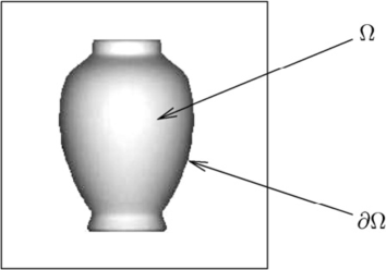
We assume that the surface is standing on a flat background so the height function, which is the unknown of the problem, will be non negative, $u:\Omega\rightarrow[0,\infty)$. We will denote by $\Omega$ the region inside the silhouette and we will assume (just for technical reasons) that $\Omega$ is an open and bounded subset of $\mathbb{R}^{2}$ (see Fig. 1).

Figure 1: An object on a flat background: $\Omega$ indicates the region inside the silhouette, $\partial\Omega$ the boundary of it.

It is well known that the SfS problem is described by the image irradiance equation (1) and depending on how we describe the function $R$ different reflection models are determined. We describe below some of them. To this end, it would be useful to introduce a representation of the brightness function $I(\mathbf{x})$ where we can distinguish different terms representing the contribution of ambient, diffuse reflected and specular reflected light. We will write then

$$I(\mathbf{x})=k_{A}I_{A}(\mathbf{x})+k_{D}I_{D}(\mathbf{x})+k_{S}I_{S}(\mathbf{x}),$$ (4)

where $I_{A}(\mathbf{x})$, $I_{D}(\mathbf{x})$ and $I_{S}(\mathbf{x})$ are respectively the above mentioned components and $k_{A}$, $k_{D}$ and $k_{S}$ indicate the percentages of these components such that their sum is equal to 1 (we do not consider absorption phenomena). Note that the diffuse or specular albedo is inside the definition of $I_{D}(\mathbf{x})$ or $I_{S}(\mathbf{x})$, respectively. In the sequel, we will always consider $I(\mathbf{x})$ normalized in $[0,1]$. This will allow to switch on and off the different contributions depending on the model. Let us note that the ambient light term $I_{A}(\mathbf{x})$ represents light everywhere in a given scene. In the whole paper we will consider it as a constant and we will neglect its contribution fixing $k_{A}=0$. Moreover, for all the models presented below we will suppose uniform diffuse and/or specular albedo and we will put them equal to $1$, that is all the points of the surface reflect completely the light that hits them. We will omit them in what follows. As we will see in the following sections, the intensity of diffusely reflected light in each direction is proportional to the cosine of the angle $\theta_{i}$ between surface normal and light source direction, without taking into account the point of view of the observer, but another diffuse model (the Oren–Nayar model) will consider it in addition. The amount of specular reflected light towards the viewer is proportional to $(\cos\theta_{s})^{\alpha}$, where $\theta_{s}$ is the angle between the ideal (mirror) reflection direction of the incoming light and the viewer direction, $\alpha$ being a constant modelling the specularity of the material. In this way we have a more general model and, dropping the ambient and specular component, we retrieve the Lambertian reflection as a special case.

3 The Lambertian model (L–model)

For a Lambertian surface, which generates a purely diffuse model, the specular component does not exist, then in (4) we have just the diffuse component $I_{D}$ on the right side. Lambertian shading is view independent, hence the irradiance equation (1) becomes

$$I(\mathbf{x})=\mathbf{N}(\mathbf{x})\cdot\boldsymbol{\omega}.$$ (5)

Under these assumptions, the orthographic SfS problem consists in determining the function $u:\overline{\Omega}\rightarrow\mathbb{R}$ that satisfies the equation (5). The unit vector $\boldsymbol{\omega}$ and the function $I(\mathbf{x})$ are the only quantities known.
For Lambertian surfaces [30, 31], just considering an orthographic projection of the scene, it is possible to model the SfS problem via a nonlinear PDE of the first order which describes the relation between the surface $u(\mathbf{x})$ (our unknown) and the brightness function $I(\mathbf{x})$. In fact, recalling the definition of the unit normal to a graph given in (3), we can write (5) as

$$I(\mathbf{x})\sqrt{1+|\nabla u(\mathbf{x})|^{2}}+\widetilde{\boldsymbol{\omega}}\cdot\nabla u(\mathbf{x})-\omega_{3}=0,\hbox{ in }\Omega$$ (6)

where $\widetilde{\boldsymbol{\omega}}=(\omega_{1},\omega_{2})$. This is an Hamilton-Jacobi type equation which does not admit in general a regular solution. It is known that the mathematical framework to describe its weak solutions is the theory of viscosity solutions as in [40].

The vertical light case.
If we choose $\boldsymbol{\omega}=(0,0,1)$, the equation (6) becomes the so-called “eikonal equation”:

$$|\nabla u(\mathbf{x})|=f(\mathbf{x})\quad\textrm{for}\quad\mathbf{x}\in\Omega,$$ (7)

where

$$f(\mathbf{x})=\sqrt{\frac{1}{I(\mathbf{x})^{2}}-1}.$$ (8)

The points $\mathbf{x}\in\Omega$ where $I(\mathbf{x})$ assumes maximum value correspond to the case in which $\boldsymbol{\omega}$ and $\mathbf{N}(\mathbf{x})$ have the same direction: these points are usually called “singular points”.
In order to make the problem well-posed, we need to add boundary conditions to the equations (6) or (7): they can require the value of the solution $u$ (Dirichlet boundary conditions type), or the value of its normal derivative (Neumann boundary conditions), or an equation that must be satisfied on the boundary (the so-called boundary conditions “state constraint”). In this paper, we consider Dirichlet boundary conditions equal to zero assuming a surface on a flat background

$$u(\mathbf{x})=0,\quad\textrm{for}\quad\mathbf{x}\in\partial\Omega,$$ (9)

but a second possibility of the same type occurs when it is known the value of $u$ on the boundary, which leads to the more general condition

$$u(\mathbf{x})=g(\mathbf{x}),\quad\textrm{for}\quad\mathbf{x}\in\partial\Omega.$$ (10)

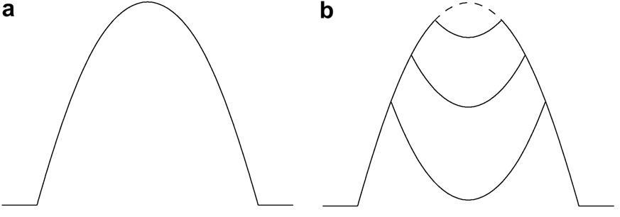
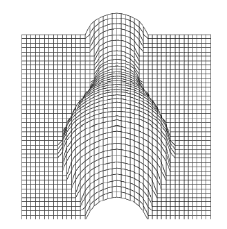
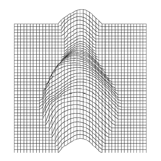
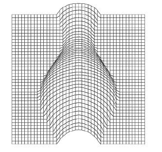
Unfortunately, adding a boundary condition to the PDE that describes the SfS model is not enough to obtain a unique solution because of the concave/convex ambiguity. In fact, the Dirichlet problem (6)-(10) can have several weak solutions in the viscosity sense and also several classical solutions due to this ambiguity (see [29]). As an example, all the surfaces represented in Fig. 2 are viscosity solutions of the same problem (7)-(9) which is a particular case of (6)-(10) (in fact the equation is $|u^{\prime}|=-2x$ with homogenous Dirichlet boundary condition). The solution represented in Fig. 2-a is the maximal solution and is smooth. All the non-smooth a.e. solutions, which can be obtained by a reflection with respect to a horizontal axis, are still admissible weak solutions (see Fig. 2-b). In this example, the lack of uniqueness of the viscosity solution is due to the existence of a singular point where the right hand side of (7) vanishes. An additional effort is then needed to define which is the preferable solution since the lack of uniqueness is also a big drawback when trying to compute a numerical solution. In order to circumvent these difficulties, the problem is usually solved by adding some information such as height at each singular point [40].

Figure 2: Illustration of the concave/convex ambiguity: (a) maximal solution and (b) a.e. solutions giving the same image. Figure adapted from [19].

For analytical and numerical reasons it is useful to introduce the exponential Kružkov change of variable [39] $\mu v(\mathbf{x})=1-e^{-\mu u(\mathbf{x})}$. In fact, setting the problem in the new variable $v$ we will have values in $[0,1/\mu]$ instead of $[0,\infty)$ as the original variable $u$ so an upper bound will be easy to find. Note that $\mu$ is a free positive parameter which does not have a specific physical meaning in the SfS problem. However, it can play an important role also in our convergence proof as we will see later (see the remark following the end of Theorem 6.1). Assuming that the surface is standing on a flat background and following [23], we can write (6) and (9) in a fixed point form in the new variable $v$. To this end let us define $\mathbf{b}^{L}:\Omega\times\partial B_{3}(0,1)\rightarrow\mathbb{R}^{2}$ and $f^{L}:\Omega\times\partial B_{3}(0,1)\times[0,1]\rightarrow\mathbb{R}$ as

$$\mathbf{b}^{L}(\mathbf{x},a):=\frac{1}{\omega_{3}}\left(I(\mathbf{x})a_{1}-\omega_{1},I(\mathbf{x})a_{2}-\omega_{2}\right),$$ (11)

$$f^{L}(\mathbf{x},a,v(\mathbf{x})):=-\frac{I(\mathbf{x})a_{3}}{\omega_{3}}(1-\mu v(\mathbf{x}))+1$$ (12)

and let $B_{3}$ denote the unit ball in $\mathbb{R}^{3}$. We obtain

Lambertian Model $$\left\{\begin{array}[]{ll}\mu v(\mathbf{x})=T^{L}(\mathbf{x},v(\mathbf{x}),\nabla v)&\hbox{for }\mathbf{x}\in\Omega,\\ v(\mathbf{x})=0&\hbox{for }\mathbf{x}\in\partial\Omega,\end{array}\right.$$ (13) where $T^{L}(\cdot):=\min\limits_{a\in\partial B_{3}}\{\mathbf{b}^{L}(\mathbf{x},a)\cdot\nabla v(\mathbf{x})+f^{L}(\mathbf{x},a,v(\mathbf{x}))\}$.

It is important to note for the sequel that the structure of the above first order Hamilton-Jacobi equation is similar to that related to the dynamic programming approach in control theory where $\mathbf{b}$ is a vector field describing the dynamics of the system and $f$ is a running cost. In that framework the meaning of $v$ is that of a value function which allows to characterize the optimal trajectories (here they play the role of characteristic curves). The interested reader can find more details on this interpretation in [21].

4 The Oren-Nayar model (ON–model)

The diffuse reflectance ON–model [48, 49, 47, 50] is an extension of the previous L–model which explicitly allows to handle rough surfaces. The idea of this model is to represent a rough surface as an aggregation of V-shaped cavities, each with Lambertian reflectance properties (see Fig. 3).
In [48] and, with more details, in [50], Oren and Nayar derive a reflectance model for several type of surfaces with different slope-area distributions. In this paper we will refer to the model called by the authors the “Qualitative Model”, a simpler version obtained by ignoring interreflections (see Section $4.4$ of [48] for more details).

Figure 3: Facet model for surface patch $dA$ consisting of many V-shaped Lambertian cavities. Figure adapted from [34].

Assuming that there is a linear relation between the irradiance of the image and the image intensity, the $I_{D}$ brightness equation for the ON–model is given by

$$I_{D}(\mathbf{x})=\cos(\theta_{i})(A+B\sin(\alpha)\tan(\beta)M(\varphi_{i},\varphi_{r}))$$ (14)

$$\hbox{where }A=1-0.5\,\sigma^{2}(\sigma^{2}+0.33)^{-1}$$ (15)

$$\hskip 28.45274ptB=0.45\sigma^{2}(\sigma^{2}+0.09)^{-1}$$ (16)

$$\hskip 28.45274ptM(\varphi_{i},\varphi_{r})=\max\{0,\cos(\varphi_{r}-\varphi_{i})\}.$$ (17)

Note that $A$ and $B$ are two non negative constants depending on the statistics of the cavities via the roughness parameter $\sigma$. We set $\sigma\in[0,\pi/2)$, interpreting $\sigma$ as the slope of the cavities. In this model (see Fig. 4), $\theta_{i}$ represents the angle between the unit normal to the surface $\mathbf{N}(\mathbf{x})$ and the light source direction $\boldsymbol{\omega}$, $\theta_{r}$ stands for the angle between $\mathbf{N}(\mathbf{x})$ and the observer direction $\mathbf{V}$, $\varphi_{i}$ is the angle between the projection of the light source direction $\boldsymbol{\omega}$ and the $x_{1}$ axis onto the $(x_{1},x_{2})$-plane, $\varphi_{\mathrm{r}}$ denotes the angle between the projection of the observer direction $\mathbf{V}$ and the $x_{1}$ axis onto the $(x_{1},x_{2})$-plane and the two variables $\alpha$ and $\beta$ are given by

$$\alpha=\max\left\{\theta_{i},\theta_{r}\right\}\hbox{ and }\beta=\min\left\{\theta_{i},\theta_{r}\right\}.$$ (18)

Since the vectors $\boldsymbol{\omega}$ and $\mathbf{V}$ are fixed and given, their projection on the incident plane is obtained considering their first two components over three (see Eq. (21)). In this way, the quantity $\max\{0,\cos(\varphi_{r}-\varphi_{i})\}$ is computed only once for a whole image.

Figure 4: Diffuse reflectance for the ON–model. Figure adapted from [34].

We define (see Fig. 4):

$$\cos(\theta_{i}) = \mathbf{N}\cdot\boldsymbol{\omega}=\frac{-\widetilde{\boldsymbol{\omega}}\cdot\nabla u(\mathbf{x})+\omega_{3}}{\sqrt{1+|\nabla u(\mathbf{x})|^{2}}}\vspace{0.2cm}$$ (19)

$$\cos(\theta_{r}) = \mathbf{N}\cdot\mathbf{V}=\frac{-\widetilde{\mathbf{v}}\cdot\nabla u(\mathbf{x})+v_{3}}{\sqrt{1+|\nabla u(\mathbf{x})|^{2}}}\vspace{0.3cm}$$ (20)

$$\cos(\varphi_{r} - \varphi_{i})=(\omega_{1},\omega_{2})\cdot(v_{1},v_{2})=\widetilde{\boldsymbol{\omega}}\cdot\widetilde{\mathbf{v}}\vspace{0.2cm}$$ (21)

$$\sin(\theta_{i}) = \sqrt{1-(\cos(\theta_{i}))^{2}}=\frac{g_{\omega}(\nabla u(\mathbf{x}))}{\sqrt{1+|\nabla u(\mathbf{x})|^{2}}}\vspace{0.2cm}$$ (22)

$$\sin(\theta_{r}) = \sqrt{1-(\cos(\theta_{r}))^{2}}=\frac{g_{v}(\nabla u(\mathbf{x}))}{\sqrt{1+|\nabla u(\mathbf{x})|^{2}}}$$ (23)

where

$$g_{\omega}(\nabla u(\mathbf{x})) := \sqrt{1+|\nabla u(\mathbf{x})|^{2}-(-\widetilde{\boldsymbol{\omega}}\cdot\nabla u(\mathbf{x})+\omega_{3})^{2}}\vspace{0.4cm}$$

$$g_{v}(\nabla u(\mathbf{x})) := \sqrt{1+|\nabla u(\mathbf{x})|^{2}-(-\widetilde{\mathbf{v}}\cdot\nabla u(\mathbf{x})+v_{3})^{2}}.$$

For smooth surfaces, we have $\sigma=0$ and in this case the ON–model reduces to the L–model. In the particular case $\boldsymbol{\omega}=\mathbf{V}=(0,0,1)$, or, more precisely, when $\cos(\varphi_{r}-\varphi_{i})\leq 0$ (e.g. the case when the unit vectors $\boldsymbol{\omega}$ and $\mathbf{V}$ are perpendicular we get $\cos(\varphi_{r}-\varphi_{i})=-1$) the equation (14) simplifies and reduces to a L–model scaled by the coefficient $A$. This means that the model is more general and flexible than the L–model. This happens when only one of the two unit vectors is zero or, more in general, when the dot product between the normalized projections onto the $(x_{1},x_{2})$-plane of $\boldsymbol{\omega}$ and $\mathbf{V}$ is equal to zero.

Also for this diffuse model we neglect the ambient component, setting $k_{D}=1$. As a consequence, in the general equation (4) the total light intensity $I(\mathbf{x})$ is equal to the diffuse component $I_{D}(\mathbf{x})$ (described by the equation (14)). This is why we write $I(\mathbf{x})$ instead of $I_{D}(\mathbf{x})$ in what follows.

To deal with this equation one has to compute the $\min$ and $\max$ operators which appear in (14) and (18). Hence, we must consider several cases described in detail in what follows. For each case we will derive a partial differential equation that is always a first order nonlinear HJ equation:

Case 1: $\theta_{i}\geq\theta_{r}$ and $(\varphi_{r}-\varphi_{i})\in[0,\frac{\pi}{2})\cup(\frac{3}{2}\pi,2\pi]$
The brightness equation (14) becomes

$$I(\mathbf{x})=\cos(\theta_{i})\left(A\!+\!B\sin(\theta_{i})\frac{\sin(\theta_{r})}{\cos(\theta_{r})}\cos(\varphi_{r}-\varphi_{i})\right)$$ (24)

and by using the formulas (19)-(23) we arrive to the following HJ equation

$$\begin{array}[]{ll}&I(\mathbf{x})(\sqrt{1+|\nabla u(\mathbf{x})|^{2}})\vspace{0.2cm}\displaystyle+A(\widetilde{\boldsymbol{\omega}}\cdot\nabla u(\mathbf{x})-\omega_{3})\vspace{0.2cm}\\ &\displaystyle-B\frac{(\widetilde{\boldsymbol{\omega}}\cdot\widetilde{\mathbf{v}})\,g_{\omega}(\nabla u(\mathbf{x}))\,g_{v}(\nabla u(\mathbf{x}))(-\widetilde{\boldsymbol{\omega}}\cdot\nabla u(\mathbf{x})+\omega_{3})}{\sqrt{1+|\nabla u(\mathbf{x})|^{2}}\,\,(-\widetilde{\mathbf{v}}\cdot\nabla u(\mathbf{x})+v_{3})}=0,\end{array}$$ (25)

where $\widetilde{\boldsymbol{\omega}}:=(\omega_{1},\omega_{2})$ and $\widetilde{\mathbf{v}}:=(v_{1},v_{2})$.


Case 2: $\theta_{i}<\theta_{r}$ and $(\varphi_{r}-\varphi_{i})\in[0,\frac{\pi}{2})\cup(\frac{3}{2}\pi,2\pi]$
In this case the brightness equation (14) becomes

$$I(\mathbf{x})=\cos(\theta_{i})\left(A\!+\!B\sin(\theta_{r})\frac{\sin(\theta_{i})}{\cos(\theta_{i})}\cos(\varphi_{r}-\varphi_{i})\right)$$ (26)

and by using again the formulas (19)-(23) we get

$$\begin{array}[]{ll}I(\mathbf{x})&(1+|\nabla u(\mathbf{x})|^{2})\vspace{0.2cm}\\ &+A(\widetilde{\boldsymbol{\omega}}\cdot\nabla u(\mathbf{x})-\omega_{3})\,\sqrt{1+|\nabla u(\mathbf{x})|^{2}}\vspace{0.2cm}\\ &-B(\widetilde{\boldsymbol{\omega}}\cdot\widetilde{\mathbf{v}})\,g_{\omega}(\nabla u(\mathbf{x}))\,g_{v}(\nabla u(\mathbf{x}))=0.\vspace{0.2cm}\end{array}$$ (27)

Case 3: $\forall\,\theta_{i},\theta_{r}$ and $(\varphi_{r}-\varphi_{i})\in[\frac{\pi}{2},\frac{3}{2}\pi]$
In this case we have the implication $\max\{0,\cos(\varphi_{r}-\varphi_{i})\}=0$. The brightness equation (14) simplifies in

$$I(\mathbf{x})=A\,\cos(\theta_{i})$$ (28)

and the HJ equation associated to it becomes consequentially

$$I(\mathbf{x})(\sqrt{1+|\nabla u(\mathbf{x})|^{2}})+A(\widetilde{\boldsymbol{\omega}}\cdot\nabla u(\mathbf{x})-\omega_{3})=0,$$ (29)

that is equal to the L–model scaled by the coefficient $A$.

Case 4: $\theta_{i}=\theta_{r}$ and $\varphi_{r}=\varphi_{i}$
This is a particular case when the position of the light source $\boldsymbol{\omega}$ coincides with the observer direction $\mathbf{V}$ but there are not on the vertical axis. This choice implies $\max\{0,\cos(\varphi_{i}-\varphi_{r})\}=1$, then defining $\theta:=\theta_{i}=\theta_{r}=\alpha=\beta$, the equation (14) simplifies to

$$I(\mathbf{x})=\cos(\theta)\ \left(A\!+\!B\sin(\theta)^{2}\cos(\theta)^{-1}\right)$$ (30)

and we arrive to the following HJ equation

$$\begin{array}[]{ll}(I(\mathbf{x})&-B)(\sqrt{1+|\nabla u(\mathbf{x})|^{2}})+A(\widetilde{\boldsymbol{\omega}}\cdot\nabla u(\mathbf{x})-\omega_{3})\vspace{0.2cm}\\ &\displaystyle+B\frac{(-\widetilde{\boldsymbol{\omega}}\cdot\nabla u(\mathbf{x})+\omega_{3})^{2}}{\sqrt{1+|\nabla u(\mathbf{x})|^{2}}}=0.\end{array}$$ (31)

Note that this four cases are exactly the same cases reported and analyzed in [35]. This is not surprising since the reflectance model used there is always the same one proposed by Oren and Nayar. However, here we get different HJ equations since we consider an orthographic camera projection and cartesian coordinates whereas in [35] the HJ equations are derived in spherical coordinates under a generalized perspective camera projection. Another major difference is that in that paper the light source is close to the camera but is not located at the optical center of the camera.

The vertical light case.
If $\boldsymbol{\omega}=(0,0,1)$, independently of the position of $\mathbf{V}$, the analysis is more simple. In fact, the first three cases considered above reduce to a single case corresponding to the following simplified PDE for the brightness equation (14)

$$I(\mathbf{x})=\displaystyle\frac{A}{\sqrt{1+|\nabla u(\mathbf{x})|^{2}}}.$$ (32)

In this way we can put it in the following eikonal type equation, analogous to the Lambertian eikonal equation (7):

$$|\nabla u(\mathbf{x})|=f(\mathbf{x})\quad\textrm{for}\quad\mathbf{x}\in\Omega,$$ (33)

where

$$f(\mathbf{x})=\displaystyle\sqrt{\frac{A^{2}}{I(\mathbf{x})^{2}}-1}.$$ (34)

Following [73], we write the surface as $S(\mathbf{x},z)=z-u(\mathbf{x})=0$, for $\mathbf{x}\in\Omega$, $z\in\mathbb{R}$, and $\nabla S(\mathbf{x},z)=(-\nabla u(\mathbf{x}),1)$, so (31) becomes

$$\begin{array}[]{ll}(I(\mathbf{x})-B)&|\nabla S(\mathbf{x},z)|\vspace{0.2cm}\\ &+A(-\nabla S(\mathbf{x},z)\cdot\boldsymbol{\omega})\vspace{0.2cm}\\ &+B\left(\frac{\nabla S(\mathbf{x},z)}{|\nabla S(\mathbf{x},z)|}\cdot\boldsymbol{\omega}\right)^{2}|\nabla S(\mathbf{x},z)|=0.\end{array}$$ (35)

Defining

$$\mathbf{d}(\mathbf{x},z):=\nabla S(\mathbf{x},z)/|\nabla S(\mathbf{x},z)|$$ (36)

and

$$c(\mathbf{x},z):=I(\mathbf{x})-B+B(\mathbf{d}(\mathbf{x},z)\cdot\boldsymbol{\omega})^{2},$$ (37)

using the equivalence

$$|\nabla S(\mathbf{x},z)|\equiv\max_{a\in\partial B_{3}}\{a\cdot\nabla S(\mathbf{x},z)\}$$ (38)

we get

$$\max_{a\in\partial B_{3}}\{c(\mathbf{x},z)\,a\cdot\nabla S(\mathbf{x},z)-A\boldsymbol{\omega}\cdot\nabla S(\mathbf{x},z)\}=0.$$ (39)

Let us define the vector field for the ON-model

$$\mathbf{b}^{ON}(\mathbf{x},a):=\frac{\left(c(\mathbf{x},z)a_{1}-A\omega_{1},c(\mathbf{x},z)a_{2}-A\omega_{2}\right)}{A\omega_{3}},$$ (40)

and

$$f^{ON}(\mathbf{x},z,a,v(\mathbf{x})):=-\frac{c(\mathbf{x},z)a_{3}}{A\omega_{3}}(1-\mu v(\mathbf{x}))+1.$$ (41)

Then, introducing the exponential Kružkov change of variable $\mu v(\mathbf{x})=1-e^{-\mu u(\mathbf{x})}$ as already done for the L–model, we can finally write the fixed point problem in the new variable $v$ obtaining the

Oren-Nayar Model $$\left\{\begin{array}[]{ll}\mu v(\mathbf{x})=T^{ON}(\mathbf{x},v(\mathbf{x}),\nabla v),&\textrm{$\mathbf{x}\in\Omega$},\\ v(\mathbf{x})=0,&\textrm{$\mathbf{x}\in\partial\Omega$.}\end{array}\right.$$ (42) where $$T^{ON}(\cdot):=\min\limits_{a\in\partial B_{3}}\{\mathbf{b}^{ON}(\mathbf{x},a)\cdot\nabla v(\mathbf{x})+f^{ON}(\mathbf{x},z,a,v(\mathbf{x}))\}$$

Note that the simple homogeneous Dirichlet boundary condition is due to the flat background behind the object but a condition like $u(\mathbf{x})=g(\mathbf{x})$ can also be considered if necessary. Moreover, the structure is similar to the previous Lambertian model although the definition of the vector field and of the cost are different.
In the particular case when $\cos(\varphi_{r}-\varphi_{i})=0$, the equation (14) simply reduces to

$$I(\mathbf{x})=A\cos(\theta)$$ (43)

and, as a consequence, the Dirichlet problem in the variable $v$ is equal to (42) with $c(\mathbf{x},z)=I(\mathbf{x})$.

5 The Phong model (PH–model)

The PH–model is an empirical model that was developed by Phong [51] in 1975. This model introduces a specular component to the brightness function $I(\mathbf{x})$, representing the diffuse component $I_{D}(\mathbf{x})$ in (4) as the Lambertian reflectance model.
A simple specular model is obtained putting the incidence angle equal to the reflection one and $\boldsymbol{\omega}$, $\mathbf{N}(\mathbf{x})$ and $\mathbf{R}(\mathbf{x})$ belong to the same plane.
This model describes the specular light component $I_{S}(\mathbf{x})$ as a power of the cosine of the angle between the unit vectors $\mathbf{V}$ and $\mathbf{R}(\mathbf{x})$ (it is the vector representing the reflection of the light $\boldsymbol{\omega}$ on the surface). Hence, the brightness equation for the PH–model is

$$I(\mathbf{x})=k_{D}(\mathbf{N}(\mathbf{x})\cdot\boldsymbol{\omega})+k_{S}(\mathbf{R}(\mathbf{x})\cdot\mathbf{V})^{\alpha},$$ (44)

where the parameter $\alpha\in[1,10]$ is used to express the specular reflection properties of a material and $k_{D}$ and $k_{S}$ indicate the percentages of diffuse and specular components, respectively. Note that the contribution of the specular part decreases as the value of $\alpha$ increases.

Starting to see in details the PH–model in the case of oblique light source $\boldsymbol{\omega}$ and oblique observer $\mathbf{V}$.
Assuming that $\mathbf{N}(\mathbf{x})$ is the bisector of the angle between $\boldsymbol{\omega}$ and $\mathbf{R}(\mathbf{x})$ (see Fig. 5), we obtain

$$\mathbf{N}(\mathbf{x})=\frac{\boldsymbol{\omega}+\mathbf{R}(\mathbf{x})}{||\boldsymbol{\omega}+\mathbf{R}(\mathbf{x})||}$$ (45)

which implies

$$\mathbf{R}(\mathbf{x})=||\boldsymbol{\omega}+\mathbf{R}(\mathbf{x})||\mathbf{N}(\mathbf{x})-\boldsymbol{\omega}.$$ (46)

From the parallelogram law, taking into account that $\boldsymbol{\omega},\mathbf{R}(\mathbf{x})$ and $\mathbf{N}(\mathbf{x})$ are unit vectors, we can write $||\boldsymbol{\omega}+\mathbf{R}(\mathbf{x})||=2(\mathbf{N}(\mathbf{x})\cdot\boldsymbol{\omega})$, then we can derive the unit vector $\mathbf{R}(\mathbf{x})$ as follow:

$$\mathbf{R}(\mathbf{x})=2(\mathbf{N}(\mathbf{x})\cdot\boldsymbol{\omega})\mathbf{N}(\mathbf{x})-\boldsymbol{\omega}$$

$$=\displaystyle 2\left(\frac{-\widetilde{\boldsymbol{\omega}}\cdot\nabla u(\mathbf{x})+\omega_{3}}{\sqrt{1+|\nabla u(\mathbf{x})|^{2}}}\right)\mathbf{N}(\mathbf{x})-(\omega_{1},\omega_{2},\omega_{3})$$ (47)

$$=\displaystyle\left(\frac{-2\widetilde{\boldsymbol{\omega}}\cdot\nabla u(\mathbf{x})+2\omega_{3}}{1+|\nabla u(\mathbf{x})|^{2}}\right)\left(-\nabla u(\mathbf{x}),1\right)-(\omega_{1},\omega_{2},\omega_{3}).$$

Figure 5: Geometry of the Phong reflection model.

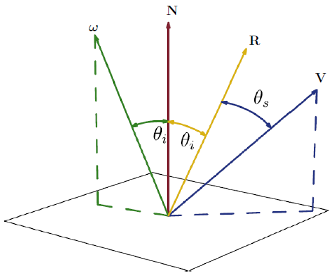
With this definition of the unit vector $\mathbf{R}(\mathbf{x})$ we have

$$\mathbf{R}(\mathbf{x})\cdot\mathbf{V}=$$ (48)

$$\displaystyle\left(\frac{-2\widetilde{\boldsymbol{\omega}}\cdot\nabla u(\mathbf{x})+2\omega_{3}}{1+|\nabla u(\mathbf{x})|^{2}}\right)\left(-\nabla u(\mathbf{x})\cdot\widetilde{\mathbf{v}}+v_{3}\right)-\boldsymbol{\omega}\cdot\mathbf{V}.$$

Then, setting $\alpha=1$, that represents the worst case, equation (44) becomes

$$I(\mathbf{x})(1+|\nabla u(\mathbf{x})|^{2})$$

$$-k_{D}(-\nabla u(\mathbf{x})\cdot\widetilde{\boldsymbol{\omega}}+\omega_{3})(\sqrt{1+|\nabla u(\mathbf{x})|^{2}})$$ (49)

$$-2k_{S}(-\nabla u(\mathbf{x})\cdot\widetilde{\boldsymbol{\omega}}+\omega_{3})\left(-\widetilde{\mathbf{v}}\cdot\nabla u(\mathbf{x})+v_{3}\right)$$

$$+k_{S}(\boldsymbol{\omega}\cdot\mathbf{V})(1+|\nabla u(\mathbf{x})|^{2})=0,$$

to which we add a Dirichlet boundary condition equal to zero, assuming that the surface is standind on a flat blackground. Note that the cosine in the specular term is usually replaced by zero if $\mathbf{R}(\mathbf{x})\cdot\mathbf{V}<0$ (and in that case we get back to the L–model).
As we have done for the previous models, we write the surface as $S(\mathbf{x},z)=z-u(\mathbf{x})=0$, for $\mathbf{x}\in\Omega$, $z\in\mathbb{R}$, and $\nabla S(\mathbf{x},z)=(-\nabla u(\mathbf{x}),1)$, so (5) will be written as

$$(I(\mathbf{x})+k_{S}(\boldsymbol{\omega}\cdot\mathbf{V}))|\nabla S(\mathbf{x},z)|^{2}$$

$$-k_{D}(\nabla S(\mathbf{x},z)\cdot\boldsymbol{\omega})(|\nabla S(\mathbf{x},z)|)$$ (50)

$$-2k_{S}(\nabla S(\mathbf{x},z)\cdot\boldsymbol{\omega})(\nabla S(\mathbf{x},z)\cdot\mathbf{V})=0.$$

Dividing by $|\nabla S(\mathbf{x},z)|$, defining $\mathbf{d}(\mathbf{x},z)$ as in (36) and $c(\mathbf{x}):=I(\mathbf{x})+k_{S}(\boldsymbol{\omega}\cdot\mathbf{V})$, we get

$$c(\mathbf{x})|\nabla S(\mathbf{x},z)|-k_{D}(\nabla S(\mathbf{x},z)\cdot\boldsymbol{\omega})$$ (51)

$$-2k_{S}(\nabla S(\mathbf{x},z)\cdot\boldsymbol{\omega})(\mathbf{d}(\mathbf{x},z)\cdot\mathbf{V})=0.$$

By the equivalence $\displaystyle|\nabla S(\mathbf{x},z)|\equiv\max_{a\in\partial B_{3}}\{a\cdot\nabla S(\mathbf{x},z)\}$ we obtain

$$\max_{a\in\partial B_{3}}\{c(\mathbf{x})\,a\cdot\nabla S(\mathbf{x},z)-k_{D}(\nabla S(\mathbf{x},z)\cdot\boldsymbol{\omega})$$ (52)

$$-2k_{S}(\nabla S(\mathbf{x},z)\cdot\boldsymbol{\omega})(\mathbf{d}(\mathbf{x},z)\cdot\mathbf{V})\}=0.$$

Let us define the vector field

$$\mathbf{b}^{PH}(\mathbf{x},a):=\frac{1}{Q^{PH}(\mathbf{x},z)}\mathbf{M}^{PH}(\mathbf{x},z)$$ (53)

where

$$Q^{PH}(\mathbf{x},z):=2k_{S}\omega_{3}(\mathbf{d}(\mathbf{x},z)\cdot\mathbf{V})+k_{D}\omega_{3},$$ (54)

and

$$\mathbf{M}_{i}^{PH}(\mathbf{x},z):=\left(c(\mathbf{x})a_{i}-k_{D}\omega_{i}\right.$$

$$\left.\hskip 48.36958pt-2k_{S}\,\omega_{i}(\mathbf{d}(\mathbf{x},z)\cdot\mathbf{V})\right),i=1,2.$$ (55)

Let us also define

$$f^{PH}(\mathbf{x},z,a,v(\mathbf{x})):=-\frac{c(\mathbf{x})a_{3}}{Q^{PH}(\mathbf{x},z)}(1-\mu v(\mathbf{x}))+1.$$ (56)

Again, using the exponential Kružkov change of variable $\mu v(\mathbf{x})=1-e^{-\mu u(\mathbf{x})}$ as done for the previous models, we can finally write the nonlinear fixed point problem

Phong Model $$\left\{\begin{array}[]{ll}\mu v(\mathbf{x})=T^{PH}(\mathbf{x},v(\mathbf{x}),\nabla v),&\textrm{$\mathbf{x}\in\Omega$},\\ v(\mathbf{x})=0,&\textrm{$\mathbf{x}\in\partial\Omega$.}\end{array}\right.$$ (57) where $$T^{PH}(\cdot):=\min\limits_{a\in\partial B_{3}}\{\mathbf{b}^{PH}(\mathbf{x},a)\cdot\nabla v(\mathbf{x})+f^{PH}(\mathbf{x},z,a,v(\mathbf{x}))\}$$

A. Oblique light source and vertical position of the observer.
In the case of oblique light source $\boldsymbol{\omega}$ and vertical observer $\mathbf{V}=(0,0,1)$, the dot product $\mathbf{R}(\mathbf{x})\cdot\mathbf{V}$ becomes

$$\begin{array}[]{ll}\mathbf{R}(\mathbf{x})\cdot\mathbf{V}&=\displaystyle\frac{-2\widetilde{\boldsymbol{\omega}}\cdot\nabla u(\mathbf{x})+2\omega_{3}}{1+|\nabla u(\mathbf{x})|^{2}}-\omega_{3}\vspace{1.0mm}\\ &\displaystyle=\frac{-2\widetilde{\boldsymbol{\omega}}\cdot\nabla u(\mathbf{x})+\omega_{3}(1-|\nabla u(\mathbf{x})|^{2})}{1+|\nabla u(\mathbf{x})|^{2}}.\end{array}$$ (58)

The fixed point problem in $v$ will be equal to (57) with the following choices

$$\begin{array}[]{lll}c(\mathbf{x})&:=&I(\mathbf{x})+\omega_{3}k_{S},\vspace{2mm}\\ Q^{PH}(\mathbf{x},z)&:=&2k_{S}(\mathbf{d}(\mathbf{x},z)\cdot\boldsymbol{\omega})+k_{D}\omega_{3},\vspace{2mm}\\ \mathbf{b}^{PH}(\mathbf{x},a)&:=&\frac{\left(c(\mathbf{x})a_{1}-k_{D}\omega_{1},c(\mathbf{x})a_{2}-k_{D}\omega_{2}\right)}{Q^{PH}(\mathbf{x},z)}\end{array}$$ (62)

B. Vertical light source and oblique position of the observer.
When $\boldsymbol{\omega}=(0,0,1)$ the definition of the vector $\mathbf{R}(\mathbf{x})$ reported in (5) becomes

$$\mathbf{R}(\mathbf{x})=\displaystyle\left(\frac{-2\nabla u(\mathbf{x})}{1+|\nabla u(\mathbf{x})|^{2}},\frac{2}{1+|\nabla u(\mathbf{x})|^{2}}-1\right)$$ (63)

and, as a consequence, the dot product $\mathbf{R}(\mathbf{x})\cdot\mathbf{V}$ with general $\mathbf{V}$ is

$$\mathbf{R}(\mathbf{x})\cdot\mathbf{V}=\frac{-2\widetilde{\mathbf{v}}\cdot\nabla u(\mathbf{x})+v_{3}(1-|\nabla u(\mathbf{x})|^{2})}{1+|\nabla u(\mathbf{x})|^{2}}.$$ (64)

Hence, the fixed point problem in $v$ is equal to (57) with

$$\begin{array}[]{lll}c(\mathbf{x})&:=&I(\mathbf{x})+v_{3}k_{S},\vspace{2mm}\\ Q^{PH}(\mathbf{x},z)&:=&2k_{S}(\mathbf{d}(\mathbf{x},z)\cdot\mathbf{V})+k_{D},\vspace{2mm}\\ \mathbf{b}^{PH}(\mathbf{x},a)&:=&\frac{1}{Q^{PH}(\mathbf{x},z)}\left(c(\mathbf{x})a_{1},c(\mathbf{x})a_{2}\right).\end{array}$$ (68)

C. Vertical light source and vertical position of the observer.
If we choose $\boldsymbol{\omega}\equiv\mathbf{V}=(0,0,1)$ the equation (5) simplifies in

$$I(\mathbf{x})(1+|\nabla u(\mathbf{x})|^{2})-k_{S}(1-|\nabla u(\mathbf{x})|^{2})$$ (69)

$$\quad-k_{D}(\sqrt{1+|\nabla u(\mathbf{x})|^{2}})=0.$$

Working on this equation one can put it in the following eikonal type form, which is analogous to the Lambertian eikonal equation (7):

$$|\nabla u(\mathbf{x})|=f(\mathbf{x})\quad\textrm{for}\quad\mathbf{x}\in\Omega,$$ (70)

where now

$$f(\mathbf{x})=\displaystyle\sqrt{\frac{k_{D}^{2}-2I_{+}(\mathbf{x})I_{-}(\mathbf{x})+k_{D}^{2}\sqrt{Q(\mathbf{x})}}{2\biggl{(}I(\mathbf{x})+k_{S}\biggr{)}^{2}}},$$ (71)

with

$$I_{+}(\mathbf{x}) := I(\mathbf{x})+k_{S},$$ (72)

$$I_{-}(\mathbf{x}) := I(\mathbf{x})-k_{S},$$ (73)

$$Q(\mathbf{x}) := k_{D}^{2}+8k_{S}^{2}+8\,I(\mathbf{x})\,k_{S}.$$ (74)

Remark on the control interpretation. The above analysis has shown that all the cases corresponding to the models proposed by Oren-Nayar and by Phong lead to a stationary Hamilton-Jacobi equation of the same form, namely

$$\mu v({\bf x})=\min\limits_{a\in\partial B_{3}}\{{\bf b}({\bf x},a)\cdot\nabla v({\bf x})+f({\bf x},z,a,v({\bf x}))\}$$

where the vector field ${\bf b}$ and the cost $f$ can vary according to the model and to the case. This gives to these models a control theoretical interpretation which can be seen as a generalization of the control interpretation for the original Lambertian model (which was related to the minimum time problem). In this framework, $v$ is the value function of a rescaled (by the Kružkov change of variable) control problem in which one wants to drive the controlled system governed by

$$\dot{y}(t)={\bf b}({\bf y}(t),a(t))$$

($a(\cdot)$ here is the control function taking values in $\partial B_{3}$) from the initial position ${\bf x}$ to the target (the silhouette of the object) minimizing the cost associated to the trajectory. The running cost associated to the position and the choice of the control will be given by $f$. More informations on this interpretation, which is not crucial to understand the application to the SfS problem presented in this paper, can be found in [21].

6 Semi-Lagrangian Approximation

Now, let us state a general convergence theorem suitable for the class of differential operators appearing in the models described in the previous sections. As we noticed, the unified approach presented in this paper has the big advantage to give a unique formulation for the three models in the form of a fixed point problem

$$\mu v(\mathbf{x})=T^{M}(\mathbf{x},v,\nabla v),\quad\hbox{for }\mathbf{x}\in\Omega,$$ (75)

where $M$ indicates the model, i.e. $M=L,ON,PH$.

We will see that the discrete operators of the ON–model and the PH–model described in the previous sections satisfy the properties listed here. In order to obtain the fully discrete approximation we will adopt the semi-Lagrangian approach described in the book by Falcone and Ferretti [21]. The reader can also refer to [12] for a similar approach to various image processing problems (including nonlinear diffusions models and segmentation).

Let $W_{i}=w(x_{i})$ so that $W$ will be the vector solution giving the approximation of the height $u$ at every node $x_{i}$ of the grid. Note that in one dimension the index $i$ is an integer number, in two dimensions $i$ denotes a multi-index, $i=(i_{1},i_{2})$. We consider a semi-Lagrangian scheme written in a fixed point form, so we will write the fully discrete scheme as

$$W_{i}=\widehat{T}_{i}(W).$$ (76)

Denoting by $G$ the global number of nodes in the grid, the operator corresponding to the oblique light source is $\widehat{T}:\mathbb{R}^{G}\rightarrow\mathbb{R}^{G}$ that is defined componentwise by

$$\widehat{T}_{i}(W):=\min\limits_{a\in\partial B_{3}}\{e^{-\mu h}I[W](x_{i}^{+})-\tau F(x_{i},z,a)\}+\tau$$ (77)

where $I[W]$ represents an interpolation operator based on the values at the grid nodes and

$$x_{i}^{+}:=x_{i}+hb(x_{i},a)$$ (78)

$$\tau:=(1-e^{-\mu\,h})/{\mu}$$ (79)

$$F(x_{i},z,a):=P(x_{i},z)a_{3}(1-\mu W_{i})$$ (80)

$$P:\Omega\times\mathbb{R}\rightarrow\mathbb{R}\hbox{ is continuous and nonnegative}.$$ (81)

Since $w(x_{i}+hb(x_{i},a))$ is approximated via $I[W]$ by interpolation on $W$ (which is defined on the grid $G$), it is important to use a monotone interpolation in order to preserve the properties of the continuous operator $T$ in the discretization. To this end, the typical choice is to apply a piecewise linear (or bilinear) interpolation operator $I_{1}[W]:\Omega\rightarrow\mathbb{R}$ which allows to define a function defined for every $x\in\Omega$ (and not only on the nodes)

$$w(x)=I_{1}[W](x)=\sum_{j}\lambda_{ij}(a)W_{j}$$ (82)

where

$$\sum_{j}\lambda_{ij}(a)=1\quad\hbox{for}\quad x=\sum_{j}\lambda_{ij}(a)x_{j}.$$ (83)

A simple explanation for (82)-(83) is that the coefficients $\lambda_{ij}(a)$ represent the local coordinates of the point $x$ with respect to the grid nodes (see [21] for more details and other choices of interpolation operators). Clearly, in (77) we will apply the interpolation operator to the point $x^{+}_{i}=x_{i}+hb(x_{i},a)$ and we will denote by $w$ the function defined by $I_{1}[W]$.

Comparing (77) with its analogue for the vertical light case we can immediately note that the former has the additional term $\tau F(x_{i},z,a)$ which requires analysis.

Theorem 6.1

Let $\widehat{T}_{i}(W)$ the $i$-th component of the operator defined as in (77). Then, the following properties hold true:

1. Let
   $\overline{a}_{3}\equiv arg\min\limits_{a\in\partial B_{3}}\{e^{-\mu h}w(x_{i}+hb(x_{i},a))-\tau F(x_{i},z,a)\}$ and assume

   $$P(x_{i},z)\overline{a}_{3}\leq 1.$$ (84)

   Then $0\leq W\leq\frac{1}{\mu}$ implies $0\leq\widehat{T}(W)\leq\frac{1}{\mu}$.
   

2. $\widehat{T}$ is a monotone operator, i.e., $W\leq\overline{W}$ implies $\widehat{T}(W)\leq\widehat{T}(\overline{W})$.
   

3. $\widehat{T}$ is a contraction mapping in $L^{\infty}([0,1/\mu)^{G})$ if

   $P(x_{i},z)\,\overline{a}_{3}<\mu$.

Proof.

1. To prove that $W\leq\frac{1}{\mu}$ implies $T(W)\leq\frac{1}{\mu}$ we just note that

   $$\widehat{T}(W)\leq\frac{e^{-\mu h}}{\mu}+\tau=\frac{1}{\mu}.$$ (85)

   Let $W\geq 0$; then

   $$\widehat{T}(W) \geq-\tau P(x_{i},z)\,\overline{a}_{3}(1-\mu W_{i})+\tau$$ (86)

   $$=\tau\left(1-P(x_{i},z)\,\overline{a}_{3}(1-\mu W_{i})\right).$$

   This implies that $\widehat{T}(W)\geq 0$ if $P(x_{i},z)\,\overline{a}_{3}\leq 1$ since $0\leq 1-\mu W_{i}\leq 1$.
   

2. In order to prove that $\widehat{T}$ is monotone, let us observe first that for each couple of functions $w_{1}$ and $w_{2}$ such that $w_{1}(x)\leq w_{2}(x)$ for every $x\in\Omega$ implies

   $$e^{-\mu h}[w_{1}(x+hb(x,a^{*}))-w_{2}(x+hb(x,\overline{a}))]\vspace{0.1cm}$$ (87)

   $$\quad-\tau P(x,z)(a^{*}_{3}(1-\mu w_{1}(x))-\overline{a}_{3}(1-\mu w_{2}(x)))$$

   $$\leq e^{-\mu h}[w_{1}(x+hb(x,\overline{a}))-w_{2}(x+hb(x,\overline{a}))]$$

   $$\quad+\tau P(x,z)\overline{a}_{3}(w_{1}(x)-w_{2}(x))$$

   where $a^{*}$ and $\overline{a}$ are the two arguments corresponding to the minimum on $a$ of the expression

   $$e^{-\mu h}w(x+hb(x,a))-\tau P(x,z)a_{3}(1-\mu w(x))$$ (88)

   respectively for $w=w_{1},w_{2}$. Hence, if we take now two vectors $W$ and $\overline{W}$ such that $W\leq\overline{W}$ and we denote respectively by $w$ and $\overline{w}$ the corresponding functions defined by interpolation, we will have $w(x)=I_{1}[W](x)\leq I_{1}[\overline{W}](x)=\overline{w}(x)$, for every $x\in\Omega$, because the linear interpolation operator $I_{1}$ is monotone. Then, by (77), setting $x_{i}^{+}=x_{i}+hb(x_{i},\overline{a})$ we get

   $$\widehat{T}_{i}(W)-\widehat{T}_{i}(\overline{W})\leq e^{-\mu h}[I_{1}[W](x_{i}^{+}))-I_{1}[\overline{W}](x_{i}^{+}))]$$

   $$+\tau P(x_{i},z)\overline{a}_{3}(W_{i}-\overline{W}_{i})\leq 0$$ (89)

   where the last inequality follows from $P\geq 0$. So we can conclude that $\widehat{T}(W)-\widehat{T}(\overline{W})\leq 0$. Note that this property does not require condition (84) to be satisfied.
   

3. Let us consider now two vectors $W$ and $\overline{W}$ (dropping the condition $W\leq\overline{W}$) and assuming

   $$P(x_{i},z)\overline{a}_{3}<\mu.$$ (90)

   To prove that $T$ is a contraction mapping note that following the same argument used to prove the second statement we can obtain (2). Then, by applying the definition of $I_{1}$, we get

   $$\widehat{T}(W)-\widehat{T}(\overline{W})\leq\left(e^{-\mu h}+\tau P(x_{i},z)\overline{a}_{3}\right)||W-\overline{W}||_{\infty}.$$

   Reversing the role of $W$ and $\overline{W}$, one can also obtain

   $$\widehat{T}(\overline{W})-\widehat{T}(W)\leq\left(e^{-\mu h}+\tau P(x_{i},z)\overline{a}_{3}\right)||W-\overline{W}||_{\infty}$$

   and conclude then that $\widehat{T}$ is a contraction mapping in $L^{\infty}$ if and only if

   $$e^{-\mu h}+\tau P(x_{i},z)\overline{a}_{3}<1$$ (91)

   and this holds true if the bound (90) is satisfied.

$\Box$

Remark on the role of $\mu$. The parameter $\mu$ can be tuned to satisfy the inequality which guarantees the contraction map property for $\widehat{T}$. This parameter adds a degree of freedom in the Kružkov change of variable and modifies the slope of $v$. However, in the practical applications we have done in our tests, this parameter has been always set to 1 so in our experience this parameter does not seem to require a fine tuning.

Remark on the choice of the interpolation operator. Although $I_{1}$ can be replaced by a high-order interpolation operator (e.g. a cubic local Lagrange interpolation), the monotonicity of the interpolation operator plays a crucial role in the proof because we have to guarantee that the extrema of interpolation polynomial stay bounded by the minimum and maximum of the values at the nodes. This property is not satisfied by quadratic or cubic local interpolation operators and the result is that this choice introduces spurious oscillations in the numerical approximation. A cure could be to adopt Essentially Non Oscillatory (ENO) interpolations. A detailed discussion on this point is contained in [21].

Remark on the minimization. In the definition of the fixed point operator $\widehat{T}$ there is a minimization over $a\in\partial B_{3}$. A simple way to solve it is to build a discretization of $\partial B_{3}$ based on a finite number of points and get the minimum by comparison. One way to do it is to discretize the unit sphere by spherical coordinates, even a small number of nodes will be sufficient to get convergence. A detailed discussion on other methods to solve the minimization problem is contained in [21].

Let us consider now the algorithm based on the fixed-point iteration

$$\left\{\begin{array}[]{ll}W^{n}&=\widehat{T}(W^{n-1}),\\ W^{0}&\textrm{given}.\end{array}\right.$$ (92)

We can state the following convergence result

Theorem 6.2

Let $W^{k}$ be the sequence generated by (92). Then the following results hold:
1. Let $W^{0}\in\mathcal{S}=\{W\in\mathbb{R}^{G}:W\geq\widehat{T}(W)\}$, then the $W^{k}$ converges monotonically decreasing to a fixed point $W^{*}$ of the $\widehat{T}$ operator;
2. Let us choose $\mu>0$ so that the condition $P(x_{i},z)\overline{a}_{3}\leq\mu$ is satisfied. Then, $W^{k}$ converges to the unique fixed point $W^{*}$ of the $\widehat{T}$. Moreover, if $W^{0}\in\mathcal{S}$ the convergence is monotone decreasing.

Proof.

1. Starting from a point in the set of super-solutions $\mathcal{S}$, the sequence is non increasing and lives in $\mathcal{S}$ which is a closed set bounded from below (by 0). Then, $W^{k}$ converges and the limit is necessarily a fixed point for $\widehat{T}$.

2. The assumptions guaranteed by Theorem 6.1 are satisfied and $\widehat{T}$ is a contraction mapping in $[0,1/\mu]$, so the fixed point is unique. The monotonicity of $\widehat{T}$ implies that starting from $W^{0}\in\mathcal{S}$ the convergence is monotone decreasing.

$\Box$

It is important to note that the change of variable allows for an easy choice of the initial guess $W^{0}\in\mathcal{S}$ for which we have the natural choice $W^{0}=(1/\mu,1/\mu,\dots,1/\mu)$ and monotonicity can be rather useful to accelerate convergence as shown in [20]. A different way to improve convergence is to apply Fast Sweeping or Fast Marching methods as illustrated in [71, 72]. A crucial role is played by boundary conditions on the boundary of $\Omega$, where usually we impose the homogeneous Dirichlet boundary condition, $v=0$. This condition implies that the shadows must not cross the boundary of $\Omega$, so the choice $\omega_{3}=0$ corresponding to an infinite shadow behind the surface is not admissible. However, other choices are possible: to impose the height of the surface on $\partial\Omega$ we can set $v=g$ or to use a more neutral boundary condition we can impose $v=1$ (state constraint boundary condition). More informations on the use of boundary conditions for these type of problems can be found in [21].

6.1 Properties of the discrete operators $\widehat{T}^{ON}$ and $\widehat{T}^{PH}$

We consider a semi-Lagrangian (SL) discretization of (42) written in a fixed point form, so we will write the SL fully discrete scheme for the ON–model as

$$W_{i}=\widehat{T}^{ON}_{i}(W),$$ (93)

where $ON$ is the acronym identifying the ON–model. Using the same notations of the previous section, the operator corresponding to the oblique light source is $\widehat{T}^{ON}:\mathbb{R}^{G}\rightarrow\mathbb{R}^{G}$ that with linear interpolation can be written as

$$\widehat{T}^{ON}_{i}(W):=\min\limits_{a\in\partial B_{3}}\{e^{-\mu h}I_{1}[W](x_{i}^{+})-\tau F^{ON}(x_{i},z,a)\}+\tau,$$

where

$$\tau:=\displaystyle\frac{1-e^{-\mu\,h}}{\mu}\vspace{0.2cm}$$

$$b^{ON}(x_{i},a):=\displaystyle\frac{1}{A\omega_{3}}\left(c(x_{i},z)a_{1}-A\omega_{1},c(x_{i},z)a_{2}-A\omega_{2}\right)\vspace{0.2cm}$$

$$c(x_{i},z):=\displaystyle I(x_{i})-B+B(d(x_{i},z)\cdot\boldsymbol{\omega})^{2}\vspace{0.2cm}$$

$$d(x_{i},z):=\displaystyle\nabla S(x_{i},z)/|\nabla S(x_{i},z)|\vspace{0.2cm}$$

$$F^{ON}(x_{i},z,a):=P^{ON}(x_{i},z)a_{3}(1-\mu W_{i}))\vspace{0.2cm}$$

$$P^{ON}(x_{i},z):=\displaystyle\frac{c(x_{i},z)}{A\omega_{3}}.$$

Note that, in general, $P^{ON}$ will not be positive but that condition can be obtained tuning the parameter $\sigma$ since the coefficients $A$ and $B$ depend on $\sigma$. This explains why in some tests we will not be able to get convergence for every value of $\sigma\in[0,\pi/2)$. Once the non negativity of $P^{ON}$ is guaranteed, we can follow the same arguments of Theorem 6.1 to check that the discrete operator $\widehat{T}^{ON}$ satisfies the three properties which are necessary to guarantee convergence as in Theorem 6.2 provided we set $P=P^{ON}$ in that statement.

For the Phong model, the semi-Lagrangian discretization of (57) written in a fixed point form gives

$$W_{i}=\widehat{T}^{PH}_{i}(W),$$ (94)

where $\widehat{T}^{PH}:\mathbb{R}^{G}\rightarrow\mathbb{R}^{G}$, that is defined componentwise by

$$\widehat{T}^{PH}_{i}(W):=\min\limits_{a\in\partial B_{3}}\{e^{-\mu h}I_{1}[W](x_{i}^{+})-\tau F^{PH}(x_{i},z,a)\}+\tau,$$

where, in the case of oblique light source and vertical position of the observer,

$$\tau:=\displaystyle\frac{1-e^{-\mu\,h}}{\mu}\vspace{0.2cm}$$

$$b^{PH}(x_{i},a):=\displaystyle\frac{\left(c(x_{i})a_{1}-k_{D}\omega_{1},c(x_{i})a_{2}-k_{D}\omega_{2}\right)}{Q^{PH}(x_{i},z)}\vspace{0.2cm}$$

$$c(x_{i}):=\displaystyle I(x_{i})+\omega_{3}k_{S}\vspace{0.2cm}$$

$$d(x_{i},z):=\displaystyle\nabla S(x_{i},z)/|\nabla S(x_{i},z)|\vspace{0.2cm}$$

$$Q^{PH}(x_{i},z):=2k_{S}(d(x_{i},z)\cdot\boldsymbol{\omega})+k_{D}\omega_{3}\vspace{0.2cm}$$

$$F^{PH}(x_{i},z,a):=P^{PH}(x_{i},z)a_{3}(1-\mu W_{i}))\vspace{0.2cm}$$

$$P^{PH}(x_{i},z):=\displaystyle\frac{c(x_{i})}{Q^{PH}(x_{i},z)}.$$

Here the model has less parameters and $P^{PH}$ will always be nonnegative. Again, following the same arguments of Theorem 6.1, we can check that the discrete operator $\widehat{T}^{PH}$ satisfies the three properties which are necessary to guarantee convergence as in Theorem 6.2 provided we set $P=P^{PH}$ in that statement.

7 Numerical Simulations

In this section we show some numerical experiments on synthetic and real images in order to analyze the behavior of the parameters involved in the ON–model and the PH–model and to compare the performances of these models with respect to the classical L–model and with other numerical methods too. All the numerical tests in this section have been implemented in language C++. The computer used for the simulations is a MacBook Pro 13” Intel Core 2 Duo with speed of 2.66 GHz and 4GB of RAM (so the CPU times in the tables refer to this specific architecture).

We denote by $\mathcal{G}$ the discrete grid in the plane getting back to the double index notation $x_{ij}$, $G:=card(\mathcal{G})=n\times m$. We define $G_{in}:=\{x_{ij}:x_{ij}\in\Omega\}$ as the set of grid points inside $\Omega$; $G_{out}:=G\setminus G_{in}$. The boundary $\partial\Omega$ will be then approximated by the nodes such that at least one of the neighboring points belongs to $G_{in}$. For each image we define a map, called mask, representing the pixels $x_{ij}\in G_{in}$ in white and the pixels $x_{ij}\in G_{out}$ in black. In this way it is easy to distinguish the nodes that we have to use for the reconstruction (the nodes inside $\Omega$) and the nodes on the boundary $\partial\Omega$ (see e.g. Fig. 6(b)).

Regarding the minimization over $a\in\partial B_{3}$ that appears in the definition of the fixed point operators associated to the models, in all the tests we discretize the unit sphere by spherical coordinates, considering 12 steps in $\theta$ and 8 in $\phi$, where $\theta$ is the zenith angle and $\phi$ is the azimuth angle.

7.1 Synthetic tests

If not otherwise specified, all the synthetic images are defined on the same rectangular domain containing the support of the image, $\Omega\equiv[-1,1]\times[-1,1]$. We can easily modify the number of the pixels choosing different values for the steps in space $\Delta\,x$ and $\Delta\,y$. The size used for the synthetic images is $256\times 256$ pixels, unless otherwise specified. $X$ and $Y$ represent the real size (e.g. for $\Omega\equiv[-1,1]\times[-1,1]$, $X=2,Y=2$). For all the synthetic tests, since we know the algebraic expression of the surfaces, the input image rendering in gray-levels is obtained using the corresponding reflectance model. This means that for each model and each value of parameter involved in it, the reconstruction will start from a different input image. Clearly, this is not possible for real images, so for these tests the input image will be always the same for all the models, independently of the values of the parameters. Moreover, we fix $\mu=1$ and we choose the value of the tolerance $\eta$ for the iterative process equal to $10^{-8}$ for the tests on synthetic images, using as stopping rule $|W^{k+1}-W^{k}|_{max}\leq\eta$, where $k+1$ denotes the current iteration. We will see that dealing with real images, sometimes we will need to increase $\eta$.

Test 1: Sphere.

For this first test we will use the semisphere defined as

$$\begin{cases}u(x,y)=\sqrt{r^{2}-x^{2}-y^{2}}&(x,y)\in G_{in},\\ u(x,y)=0&(x,y)\in G_{out},\end{cases}$$ (95)

where

$$G_{in}:=\{(x,y):x^{2}+y^{2}\leq r^{2}\},$$ (96)

$$r:=\frac{\min\{X,Y\}}{2}+{2\,\tilde{\delta}},$$ (97)

and $\tilde{\delta}:=\max\{\Delta{}x,\Delta{}y\}$.

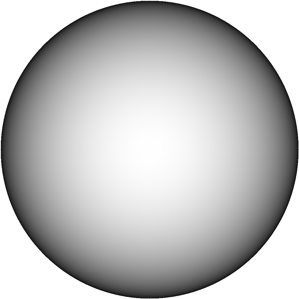
As example, we can see in Fig. 6 the input image, the corresponding mask and the surface reconstructed by the L–model.

(a) Sphere Input

(b) Sphere Mask

(c) Sphere surface

Figure 6: Sphere via the L–model: (a) Input image; (b) Mask; (c) surface.

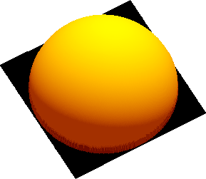
The values of the parameters used in the simulations are indicated in Table 1. Note (in Table 3) that when the specular component is zero for the PH–model, we just have the contribution of the diffuse component so we have exactly the same error values of the L–model, as expected. By increasing the value of the coefficient $k_{S}$ and, as a consequence, decreasing the value of $k_{D}$, in the PH–model the $L^{2}(I)$ and $L^{\infty}(I)$ errors on the image grow albeit slightly and still remain of the same order of magnitude, whereas the errors on the surface decrease. For the ON–model, the same phenomenon appears when we set the roughness parameter $\sigma$ to zero: we bring back to the L–model and, hence, we obtain the same errors on the image and the surface. Note that the errors in $L^{2}(I)$ and $L^{\infty}(I)$ norm for the image and the surface, decrease by increasing the value of $\sigma$. This seem to imply that the model and the approximation work better for increasing roughness values.

We point out that the errors computed on the images $I$ in the different norms are over integer between the input image and the image computed a posteriori using the value of $u$ just obtained by the methods. This is why small errors becomes bigger since can jump from an integer to the other one, as for the Phong case.

Table 1: Sphere: parameter values used in the models.

Model	$\sigma$	$k_{D}$	$k_{S}$	$\alpha$
LAM
ON-00	0
ON-04	0.4
ON-08	0.8
PH-s00		1	0	1
PH-s04		0.6	0.4	1
PH-s08		0.2	0.8	1

In Table 2 we reported the number of iterations and the CPU time (in seconds) referred to the three models with the parameter indicated in Table 1. For all the models, also varying the parameters involved, the number of iterations is always about $2000$ e the CPU time slightly greater than $2$ seconds, so the computation is really fast.

Table 2: Synthetic sphere: iterations and CPU time in seconds for the models with vertical light source $\boldsymbol{\omega}=(0,0,1)$.

SL–Schemes	Iter.	$[sec.]$
LAM	2001	2.14
ON-00	2001	2.06
ON-04	2020	2.24
ON-08	2016	2.24
PH-s00	2001	2.11
PH-s04	2008	2.45
PH-s08	2056	2.27

Table 3: Synthetic sphere: $L^{2}$, $L^{\infty}$ errors with vertical light source $\boldsymbol{\omega}=(0,0,1)$.

SL–Schemes	$L^{2}(I)$	$L^{\infty}(I)$	$L^{2}(S)$	$L^{\infty}(S)$
LAM	0.0046	0.0431	0.0529	0.0910
ON-00	0.0046	0.0431	0.0529	0.0910
ON-04	0.0039	0.0353	0.0513	0.0882
ON-08	0.0035	0.0314	0.0506	0.0881
PH-s00	0.0046	0.0431	0.0529	0.0910
PH-s04	0.0064	0.0471	0.0511	0.0896
PH-s08	0.0090	0.0706	0.0386	0.0752

Test 2: Ridge tent.

In tests on synthetic images, the relevance of the choice of a model depends on which model was used to compute the images. In the previous test, the parameters that are used for the 3D reconstruction are identical to those used to compute the synthetic sphere input images, so there is a perfect match. However, for real applications, it is relevant to examine the influence of an error in the parameter values. To this end we can produce an input image with the Oren-Nayar model using $\sigma=0.1$ and then process this image with the same model using a different value of $\sigma$ to see how the results are affected by this error. This is what we are going to do for the ridge tent. Let us consider the ridge tent defined by the following equation

$$\begin{cases}u(x,y)=\min\left\{-2\,|x|+\frac{4}{5}\,X,-|y|+\frac{2}{5}\,Y\right\}&\\ &(x,y)\in G_{in},\\ u(x,y)=0&(x,y)\in G_{out},\end{cases}$$ (98)

where

$$G_{in}:=\left\{(x,y):\frac{x}{X},\frac{y}{Y}<\frac{2}{5}\right\}.$$

In Fig. 7 we can see an example of reconstruction obtained by using the ON–model with $\sigma=0.3$, under a vertical light source $\boldsymbol{\omega}=(0,0,1)$.

(a) Tent Input

(b) Tent surface

Figure 7: Tent via the ON–model with $\sigma=0.3$: (a) Input image; (b) 3D reconstruction.

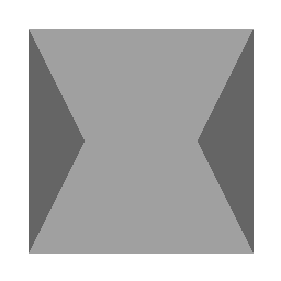
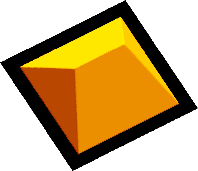
A first remark is that the surface reconstruction is good even if in this case the surface is not differentiable. Moreover, note that there are no oscillations near the kinks where there is jump in the gradient direction. Let us examine the stability with respect to the parameters. We have produced seven input images for the ridge tent, all of size $256\times{}256$, with the following combinations of models and parameters:

LAM Lambertian model;

ON1 Oren-Nayar model with $\sigma=0.1$;

ON3 Oren-Nayar model with $\sigma=0.3$;

ON5 Oren-Nayar model with $\sigma=0.5$;

PH1 Phong model with $\alpha=1$ and $k_{S}=0.1$;

PH3 Phong model with $\alpha=1$ and $k_{S}=0.3$;

PH5 Phong model with $\alpha=1$ and $k_{S}=0.5$.

Then we have computed the surfaces corresponding to all the parameter choices (i.e. matching and not matching the first choice). The results obtained in this way have been compared in terms of $L^{2}$ and $L^{\infty}$ norm errors with respect to the original surface. The errors obtained by the ON–model are shown in Table 4 and in Table 5 for the PH–model.

Table 4: Ridge tent, ON–model: $L^{2},L^{\infty}$ errors for the surface. In each column the model used to produce the input image, in the row the model used for the $3D$ reconstruction.

$L^{2}$	LAM	ON1	ON3	ON5
LAM	0.0067	0.0172	0.0933	0.1920
ON1	0.0082	0.0068	0.0821	0.1801
ON3	0.0832	0.0700	0.0086	0.1033
ON5	0.1946	0.1784	0.0923	0.0067
$L^{\infty}$	LAM	ON1	ON3	ON5
LAM	0.0094	0.0315	0.1942	0.4060
ON1	0.0199	0.0093	0.1701	0.3805
ON3	0.1784	0.1507	0.0118	0.2156
ON5	0.4104	0.3769	0.1976	0.0094

Table 5: Ridge tent, PH-model: $L^{2},L^{\infty}$ errors for the surface. In each column the model used to produce the input image, on the row the model used for the $3D$ reconstruction.

$L^{2}$	LAM	PH1	PH3	PH5
LAM	0.0067	0.0841	0.2867	0.6146
PH1	0.0586	0.0067	0.1996	0.5031
PH3	0.1403	0.0955	0.0073	0.2687
PH5	0.1915	0.1664	0.0976	0.0060
$L^{\infty}$	LAM	PH1	PH3	PH5
LAM	0.0094	0.1740	0.6068	1.3123
PH1	0.1243	0.0108	0.4202	1.0741
PH3	0.3167	0.2245	0.0149	0.5718
PH5	0.4503	0.4241	0.2907	0.0093

Analyzing the errors in Table 4 and Table 5, we can observe that using the same model to generate the input image and to reconstruct the surface is clearly the optimal choice. The errors on the surface grow more as we consider a parameter $\sigma$ other than the one used to generate the input image as data for the 3D reconstruction. For the ON–model we loose one or two order of magnitude, depending on the “distance” of the parameter from the source model. For the PH–model we can observe that the $L^{2}$ and $L^{\infty}$ errors grow more as we consider a different $k_{S}$ for the generation of the image and for the reconstruction, loosing one or two order of magnitude. However, the two models seems to be rather stable with respect to a variation of the parameters since the errors do not increase dramatically varying the parameters.

Test 3: Concave/convex ambiguity for the ON–model.

We consider this test in order to show that the ON–model is not able to overcome the concave/convex ambiguity typical of the SfS problem although it is a model more realistic than the classical L–model. Let consider the following function

$$u(x,y)=\left\{\begin{array}[]{ll}-(1-(x^{2}-y^{2}))^{2}+1,&\\ &\hbox{if }(x^{2}+y^{2})<2,\\ 0&\hbox{ otherwise}.\end{array}\right.$$ (99)

Figure 8: Example of concave/convex ambiguity for the ON–model with $\sigma=0.5$ and $\boldsymbol{\omega}=(0,0,1)$: (a) Original Surface; (b) Maximal Solution; (c) Approximated surface with value in the origin equal to zero.

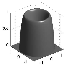
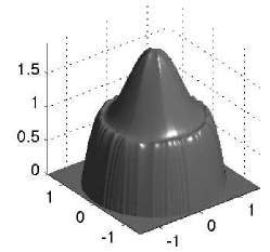
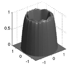
We discretize the domain $\Omega=[-1.5,1.5]\times[-1.5,1.5]$ with $151\times 151$ nodes. The fixed point has been computed with an accuracy of $\eta=10^{-4}$ and the stopping rule for the algorithm based on the fixed point iteration defined in (92) is $|W^{k+1}-W^{k}|_{max}\leq\eta$, where $k+1$ denotes the current iteration. The iterative process starts with $W^{0}=0$ on the boundary and $W^{0}=1$ inside in order to proceed from the boundary to the internal constructing a monotone sequence (see [7, 23] for details on the approximation of maximal solutions).

Looking at Fig. 8 we can note that the scheme chooses the maximal viscosity solution stopping after 105 iterations, which does not coincide with the original surface. In order to obtain a reconstruction closer to the original surface, we fix the value in the origin at zero. In this way we forced the scheme to converge to a solution different from the maximal solution (see Fig. 8). We obtained this different solution shown in Fig. 8 after 82 iterations.

Test 4: Concave/convex ambiguity for the PH–model.

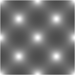
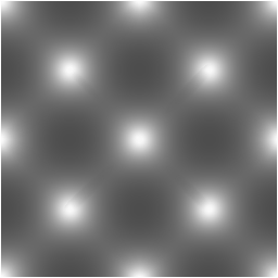
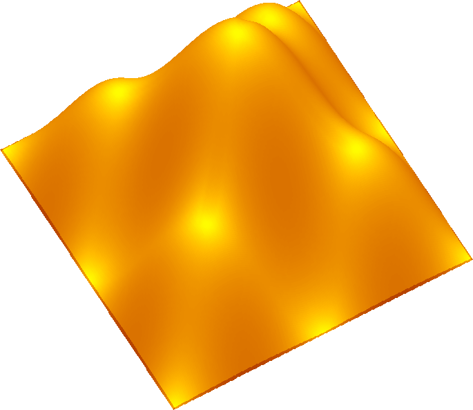
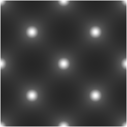
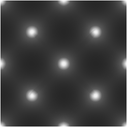
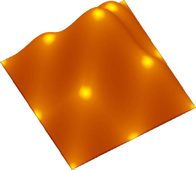
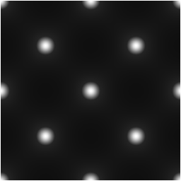
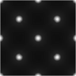
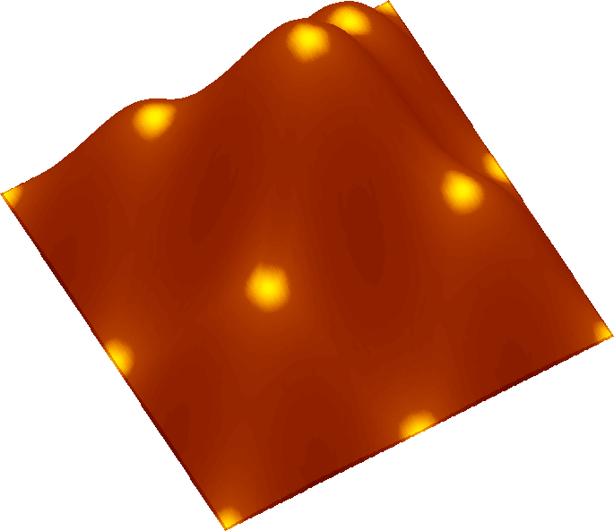
The fourth synthetic numerical experiment is related to the sinusoidal function defined as follow

$$\begin{cases}u(x,y)=\displaystyle 0.5+0.5\,\sin(\frac{\pi\,x}{\Delta x})\,\sin(\frac{\pi\,y}{\Delta y}),&\\ &(x,y)\in G_{in},\\ u(x,y)=0,&(x,y)\in G_{out}.\end{cases}$$ (100)

With this test we want to show that also the PH–model is not able to overcome the concave/convex ambiguity typical of the SfS problem.

in	out	reconstruction

Figure 9: Synthetic sinusoidal function: example of concave/convex ambiguity for the PH–model with $k_{S}=0,0.5,0.8$ for each row from the top to the bottom, respectively.

Fig. 9 shows the results related to the PH–model with $k_{S}=0,0.5,0.8$. In the first column one can see the input images generated by the PH–model using the values of the parameter before mentioned. In the second column we can see the output images computed a posteriori using the depth just computed and approximating the gradient via finite difference solver. What we can note is that even if the reconstructed a posteriori images match with the corresponding input images, the SL method always chooses the maximal solution even varying the parameters $k_{D}$ and $k_{S}$. By adding some informations as shown in the previous test it is possible to achieve a better result, but these additional informations are not available for real images.

Test 5: Role of the boundary conditions.

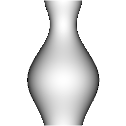
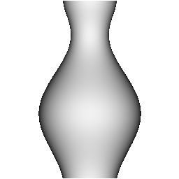
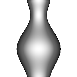
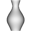
With this fifth test we want to point out the role of the boundary condition (BC), showing how good BC can significantly improve the results on the 3D reconstruction. We will use the synthetic vase defined as follow

$$\begin{cases}u(x,y)=\sqrt{P(\bar{y})^{2}-x^{2}}&(x,y)\in G_{in}\\ u(x,y)=g(x,y)&(x,y)\in G_{out},\end{cases}$$ (101)

where $\bar{y}:=y/Y$,

$$P(\bar{y}):= (-10.8\,\bar{y}^{6}+7.2\,\bar{y}^{5}+6.6\,\bar{y}^{4}-3.8\,\bar{y}^{3}$$

$$-1.375\,\bar{y}^{2}+0.5\,\bar{y}+0.25)\,X$$

and

$$G_{in}:=\{(x,y)|P(\bar{y})^{2}>x^{2}\}.$$

In Fig. 10 one can see on the first row the input images (size $256\times 256$) generated by the L–model, ON–model and the PH–model, from left to right respectively. On the second row we reported the 3D reconstruction with homogeneous Dirichlet BC ($g(x,y)=0$). As we can see, there is a concave/convex ambiguity in the reconstruction of the surface. If we consider the correct boundary condition, that is the height of the surface at the boundary of the silhouette that we can easily derive in this case being the object a solid of rotation, what we obtain is visible in the third row of the same Fig. 10.

L–model	ON–model	PH–model

Figure 10: Synthetic vase under vertical light source ($\boldsymbol{\omega}=(0,0,1)$): example of concave/convex ambiguity solved by using correct Dirichlet BC. On the first row from left to right: input images generated by L–model, ON–model with $\sigma=0.2$ and PH–model with $k_{S}=0.4$. On the second row: 3D reconstruction with homogeneous Dirichlet BC. On the last row: 3D reconstruction with Dirichlet BC $u(x,y)=g(x,y)$.

In Tables 6 and 7 we can see the number of iterations, the CPU time and the error measures in $L^{2}$ and $L^{\infty}$ norm for the method used with homogeneous and not homogeneous Dirichlet BC respectively. Looking at these errors we can note that in each table the values are almost the same for the different models. Comparing the values of the two tables one can see that we earn an order of magnitude using good BC, that confirms what we noted looking at Fig. 10.

Table 6: Synthetic Vase: Number of iterations, CPU time in seconds and $L^{2}$, $L^{\infty}$ errors on the surface with vertical light source $\boldsymbol{\omega}=(0,0,1)$ using homogeneous Drichlet BC.

SL–Schemes	Iter.	[sec.]	$L^{2}(S)$	$L^{\infty}(S)$
LAM	1010	0.54	0.1614	0.3015
ON-02	1011	0.53	0.1613	0.3015
ON-04	1008	0.54	0.1610	0.3015
PH-s02	1007	0.54	0.1619	0.3015
PH-s04	1009	0.55	0.1621	0.3015

Table 7: Synthetic Vase: Number of iterations, CPU time in seconds and $L^{2}$, $L^{\infty}$ errors on the surface with vertical light source $\boldsymbol{\omega}=(0,0,1)$ using not homogeneous Drichlet BC.

SL–Schemes	Iter.	[sec.]	$L^{2}(S)$	$L^{\infty}(S)$
LAM	1337	0.70	0.0286	0.0569
ON-02	1335	0.70	0.0284	0.0558
ON-04	1341	0.70	0.0282	0.0562
PH-s02	1330	0.70	0.0284	0.0560
PH-s04	1330	0.70	0.0280	0.0558

Test 6: Comparison with other numerical approximations.

In this sixth and last test of this section dedicated to synthetic tests we will compare the performance of our semi-Lagrangian approach with other methods used in the literature. For this reason, we will use a very common image used in the literature, that is the vase, defined in the previous test through the (101). More in details, we will compare the performance of our semi-Lagrangian method with the Lax-Friedrichs Sweeping (LFS) scheme adopted by Ahmed and Farag [1] under vertical and oblique light source. Also these authors derive some similar HJ equations for the L–model in [2], and generalize this approach for various image conditions in [1], comparing their results on the only L–model with the results shown in [63] and the algorithms reported in [85]. Unfortunately, we cannot compare our semi-Lagrangian approximation for the PH–model with no other schemes since, to our knowledge, there are no table of errors for the PH–model under orthographic projection in the literature. In order to do the comparison, we will consider the vase image of size $128\times 128$ as used in the other papers. We start to remind the error estimations used: given a vector $\mathbf{A}$ representing the reference depth map on the grid and a vector $\widetilde{\mathbf{A}}$ representing its approximation, we define the error vector as $\mathbf{e}=\mathbf{A}-\widetilde{\mathbf{A}}$ and

$$err_{1}:=||\mathbf{e}||_{L^{1}} =\frac{1}{N}\sum_{i}|e_{i}|$$

$$err_{2}:=||\mathbf{e}||_{L^{2}} =\left\{\frac{1}{N}\sum_{i}|e_{i}|^{2}\right\}^{1/2}$$

where $N$ is the total number of grid points used for the computation, i.e. the grid points belonging to $G_{in}$. These estimators are called mean and standard deviation of the absolute error. In Table 8 we compare the error measures for the different SfS algorithms under the L–model with $\boldsymbol{\omega}=(0,0,1)$. What we can note is that our semi-Lagrangian method is better than the other ones also if we consider Dirichlet boundary condition equal to zero (as used by Ahmed and Farag in their work [1]), but the better result is with correct BC, shown in bold in the last row.

Table 8: Synthetic vase: error measures related to the different methods for the L–model with vertical light source $\boldsymbol{\omega}=(0,0,1)$. In bold the best performances.

Methods	$err_{1}$	$err_{2}$
Best [85]	8.1	11.1
[63]	2.8	2.0
[1]	0.22	0.4
Our proposed ($BC=0$)	0.1570	0.1717
Our proposed ($BC\not=0$)	0.0349	0.0385

In Table 9 we can see the same methods applied to the L–model but under a different light source, that is $(1,0,1)$. Also in this case, our approach obtains always the smallest errors and the best is with not homogeneous Dirichlet BC, as noted before.

Table 9: Synthetic vase: error measures related to the different methods for the L–model with oblique light source $(1,0,1)$. In bold the best performances.

Methods	$err_{1}$	$err_{2}$
Best [85]	7.9	13.9
[63]	4.1	2.6
[1]	1.2	2.2
Our proposed ($BC=0$)	0.0683	0.1061
Our proposed ($BC\not=0$)	0.0218	0.0242

Only with respect to the LFS used by Ahmed and Farag, we can compare the performance of our semi-Lagrangian scheme under the ON–model as well, since the other authors only consider the L–model. In this context, we show in Table 10 the error measures for the two SfS algorithms with $\sigma=0.2$, under vertical position of light source and viewer ($\boldsymbol{\omega}=(0,0,1),\mathbf{V}=(0,0,1)$).

Table 10: Synthetic vase: error measures related to the SL and LFS methods for the ON–model with $\sigma=0.2$ under vertical light source ($\boldsymbol{\omega}=(0,0,1)$) and vertical viewer $\mathbf{V}=(0,0,1)$. In bold the best performances.

Methods	$err_{1}$	$err_{2}$
[1]	0.6	1.0
Our proposed ($BC=0$)	0.1568	0.1715
Our proposed ($BC\not=0$)	0.0348	0.0384

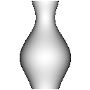
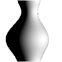
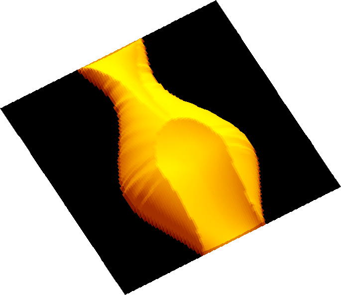
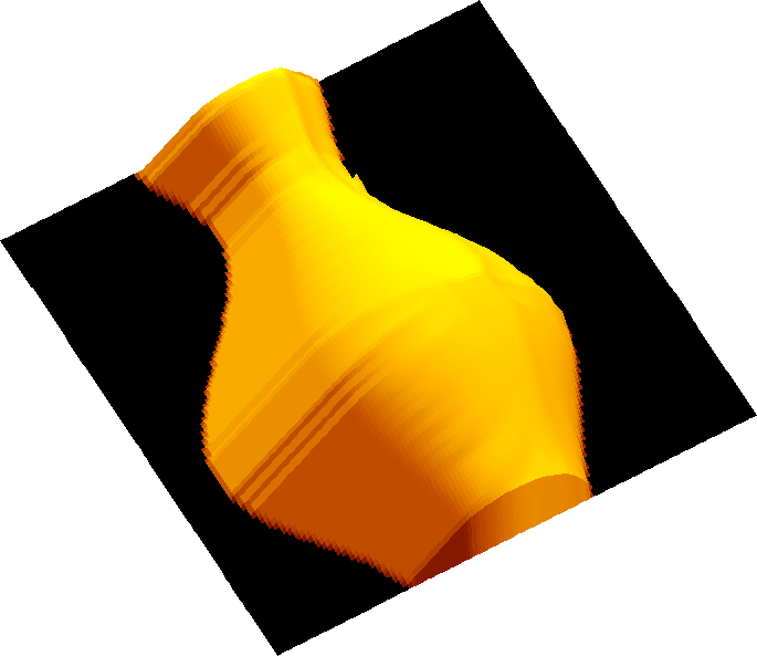
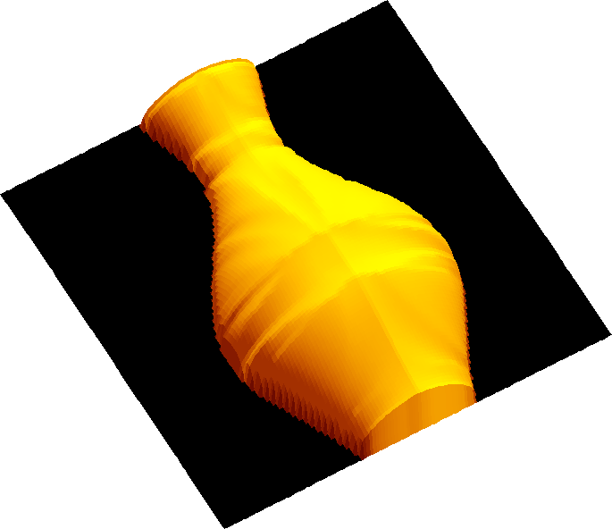
As before, the best result is obtained using the semi-Lagrangian scheme with not homogeneous Dirichlet BC. The reconstructions corresponding to the error measures shown in the three last Tables 8, 9, 10 obtained applying our scheme and compared to [1] are shown in Fig. 11. The reconstruction obtained by the two methods are comparable. In particular, in the second column regarding the oblique light source case we can note that our scheme reconstructs a surface that incorporates the black shadow part (see [23] for more details on this technique), avoiding the effects of “dent” present in the reconstruction obtained by Ahmed and Farag visible in the last row, second column.

L–model	L–model	ON–model
vertical	oblique	vertical

Figure 11: Synthetic vase: From top to bottom, Input images, recovered shapes by our approach with homogeneous Dirichlet BC and with not homogeneous BC, recovered shape by [1]. First column: L–model with vertical light source (0,0,1). Second column: L–model with oblique light source (1,0,1). Third column: ON–model with $\sigma=0.2$, $\boldsymbol{\omega}=(0,0,1)$, $\mathbf{V}=(0,0,1)$. Input images size: $128\times 128$.

Finally, in Table 11 we reported the number of iterations and the CPU time in seconds with the comparison with respect to [1].

Table 11: Synthetic vase: iterations and CPU time in seconds for the L–model and the ON–model with vertical light source $\boldsymbol{\omega}=(0,0,1)$. Image size: $128\times 128$.

Schemes	Model	Iter.	$[sec.]$
[1]	L–model	-	0.5
Our approach ($BC=0$)	L–model	611	0.09
Our approach ($BC\not=0$)	L–model	792	0.11
[1]	ON–model	-	1.5
Our approach ($BC=0$)	ON–model	612	0.09
Our approach ($BC\not=0$)	ON–model	791	0.12

This shows that the SL-scheme is competitive also in terms of CPU time. Of course, in the case of oblique light source the number of iterations, and hence the CPU time needed is much more bigger. Just think that for the reconstruction under the L–model with oblique light source $(1,0,1)$ and $BC\not=0$ visible in the second column of the third row of Fig. 11, we need $15513$ iterations (CPU time: 147.40 seconds). If we double the size of the input image, considering the vase $256\times 256$ visible in Fig. 10, for the reconstruction visible in the third row, first column of the same Fig. 10, we need 30458 iterations to get convergence, that we obtain in 1163 seconds.

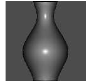
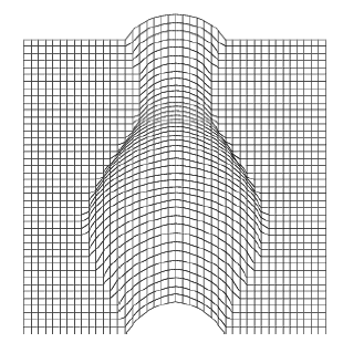
Since it is difficult to compare the performance of our approach based on the PH–model with other schemes based on the same reflectance model under orthographic projection for the consideration made before, we report in Fig. 12 the performances obtained by our method based on the PH–model compared to the approximate Ward’s method on the vase test (Cf. Fig. 7 in [1]). What we can see is that both the two methods reconstruct the surface in a quite good way, without particular distinctions in the goodness of the reconstructions. In order to analyze the results not only in a qualitative way but also in a quantitative one, we report the mean and the standard deviation of the absolute errors in Table 12. Looking at this table, we can note that our approach seems to be superior, obtaining the reconstruction with errors smaller of one order with respect to the other model.

Input	reconstruction

Figure 12: Synthetic vase: The first row shows the input image and the recovered shape by our approach with not homogeneous BC based on the PH–model with $k_{S}=0.2$, $\boldsymbol{\omega}=(0,0,1)$ and $\mathbf{V}=(0,0,1)$. The second row shows the input image and the recovered shape by the approximate Ward’s method illustrated in [1] with $\sigma=0.2$, $\rho_{d}=0.67$, $\rho_{s}=0.075$, $\boldsymbol{\omega}=(0,0,1)$, $\mathbf{V}=(0,0,1)$. Input images size: $128\times 128$.

Table 12: Synthetic vase: error measures related to the cases shown in Fig. 12. In bold the best performances.

Methods	$err_{1}$	$err_{2}$
Ward in [1]	0.8	1.3
PH–model	0.03	0.04

7.2 Real tests

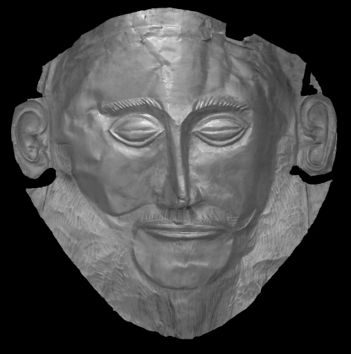
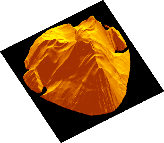
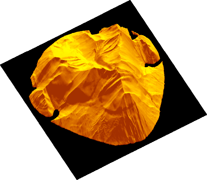
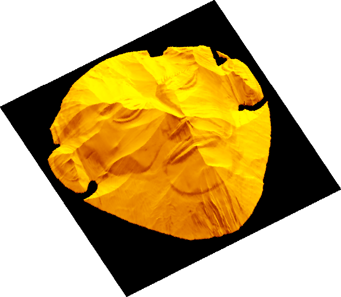
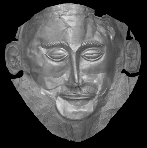
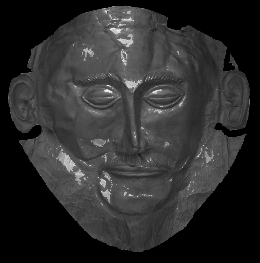
In this subsection we consider real input images. We start considering the golden mask of Agamemnon taken from [78] and then modified in order to get a picture in gray tones. The size of the modified image really used is $507\times 512$. The input image is visible in Fig. 13(a), the associated mask used for the 3D reconstruction in Fig. 13(b). The second real test is concerning the real vase (RV in the following) visible in Fig. 16, taken from [19]. The size of the input image shown in Fig. 16(a) is $256\times 256$. The reconstruction domain $\Omega_{RV}$, shown in Fig. 16(b), is constituted by the pixels situated on the vase. For the real cases, the input image is the same for all the models and we can compute only errors on the images since we do not know the height of the original surface. For the real tests we will use the same stopping criterion for the iterative method before defined for the synthetic tests, i.e. $|W^{k+1}-W^{k}|_{max}\leq\eta$.

Test 7: Agamennon mask.

(a) Agamemnon Input

(b) Agamemnon Mask

Figure 13: Agamemnon images (size $507\times 512$): (a) Input image; (b) Mask.

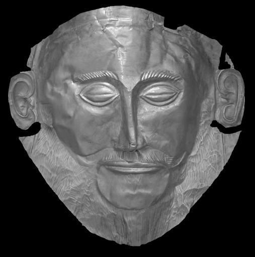
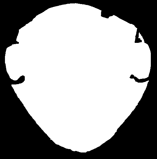
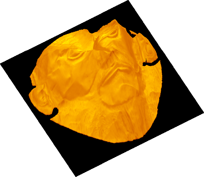
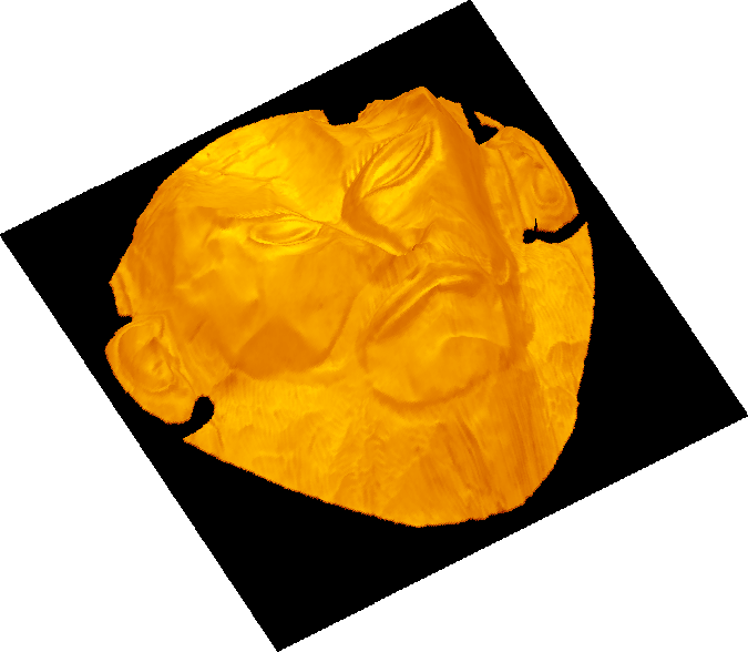
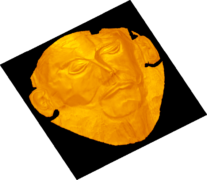
For this test we will compare the results regarding 3D reconstruction of the surface obtained with a vertical light source $\boldsymbol{\omega}_{vert}=(0,0,1)$ and an oblique light source $\boldsymbol{\omega}_{obl}=(0,0.0995,0.9950)$.

Table 13: Real Agamemnon mask: parameter values used in the models with vertical light source $\boldsymbol{\omega}=(0,0,1)$.

Model	$\sigma$	$k_{D}$	$k_{S}$	$\alpha$
LAM
ON-04	0.4
ON-08	0.8
ON-10	1
PH-s04		0.6	0.4	1
PH-s08		0.2	0.8	1
PH-s10		0	1	1

The values of the parameters used in this test are reported in Table 13. For a vertical light source, we refer to Table 14 for the number of iterations and the CPU time (in seconds) and to Table 15 for the errors obtained with a tolerance $\eta=10^{-8}$ for the stopping rule of the iterative process. Clearly, the number of iteration and the errors of the two non-Lambertian models are the same of the classical Lambertian model when $\sigma$ for the ON–model and $k_{S}$ for the PH–model are equal to zero (and for this reason we do not report them in the tables). In all the other cases, the non-Lambertian models are faster in terms of CPU time and need a lower number of iterations with respect to the L–model.

Table 14: Real Agamemnon mask: iterations and CPU time in seconds for the models with vertical light source $\boldsymbol{\omega}=(0,0,1)$.

SL–Schemes	Iter.	$[sec.]$
LAM	3921	24.48
ON-04	2751	12.48
ON-08	1943	11.41
ON-10	1818	8.79
PH-s04	2127	9.89
PH-s08	1476	6.90
PH-s10	1325	6.33

In Table 15 we can observe that the $L^{2}$ errors produced by the ON–model increase by increasing the value of $\sigma$. However, the $L^{\infty}$ errors are lower than the error obtained with the Lambertian model. With respect to the PH–model, all the errors increase by increasing the value of the parameter $k_{S}$, as observed for synthetic images.

Table 15: Real Agamemnon mask: $L^{2}$, $L^{\infty}$ errors with vertical light source $\boldsymbol{\omega}=(0,0,1)$.

SL–Schemes	$L^{2}(I)$	$L^{\infty}(I)$
LAM	0.0371	0.4745
ON-04	0.0375	0.4627
ON-08	0.0440	0.4627
ON-10	0.0501	0.4627
PH-s04	0.0383	0.4824
PH-s08	0.0391	0.4941
PH-s10	0.0393	0.5098

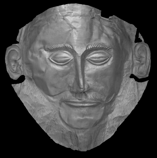
In Fig. 14 we can see the output image and the 3D reconstruction in a single case for each models. What we can note is that no big improvements we can obtain visually.

LAM	ON4	PH4

Figure 14: Agamennon mask: results with vertical light source. On the first row the output images, on the second row the 3D reconstruction with vertical view, on the third row the 3D reconstruction with oblique view.

For the oblique light case, we consider the values for the parameters reported in Table 16.

Table 16: Real Agamemnon mask: parameter values used in the models with an oblique light source $\boldsymbol{\omega}_{obl}=(0,0.0995,0.9950)$.

Model	$\sigma$	$k_{D}$	$k_{S}$	$\alpha$
LAM
ON-01	0.1
ON-02	0.2
ON-03	0.3
PH-s02		0.8	0.2	1
PH-s03		0.7	0.3	1
PH-s04		0.6	0.4	1

Looking at Table 17 we can note that the oblique cases require higher CPU time with respect to the vertical cases due to the fact that the equations are more complex because of additional terms involved. Because of these additional terms involved in the oblique case, in Table 18 we have reported the results obtained using the parameters shown in Table 16 with a value of the tolerance $\eta$ for the stopping rule of the iterative method equal to $10^{-3}$. This is the maximum accuracy achieved by the non-Lambertian models since roundoff errors coming from several terms occur and limit the accuracy.

Table 17: Real Agamemnon mask: number of iterations and CPU time in seconds for the different models with oblique light source $\boldsymbol{\omega}_{obl}=(0,0.0995,0.9950)$.

SL–Schemes	Iter.	$[sec.]$
LAM	321	117.9
ON-01	315	246.0
ON-02	361	281.5
ON-03	396	264.6
PH-s02	427	285.2
PH-s03	564	373.6
PH-s04	680	484.1

Table 18: Real Agamemnon mask: $L^{2}$, $L^{\infty}$ errors with oblique light source $\boldsymbol{\omega}_{obl}=(0,0.0995,0.9950)$.

SL–Schemes	$L^{2}(I)$	$L^{\infty}(I)$
LAM	0.0585	0.4863
ON-01	0.0663	0.4588
ON-02	0.0670	0.4471
ON-03	0.0708	0.5451
PH-s02	0.1141	0.5725
PH-s03	0.1580	0.6196
PH-s04	0.2063	0.6706

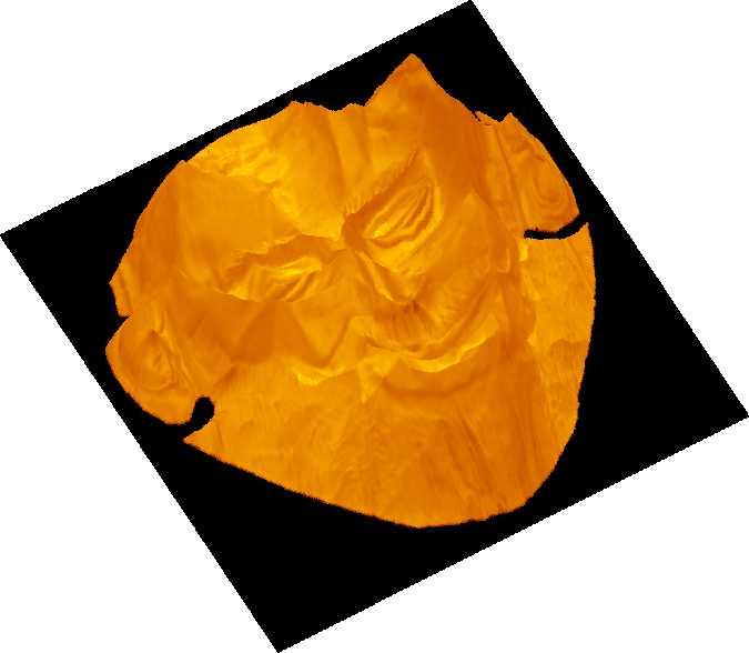
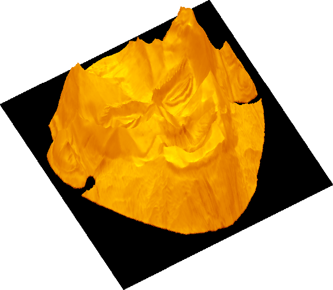
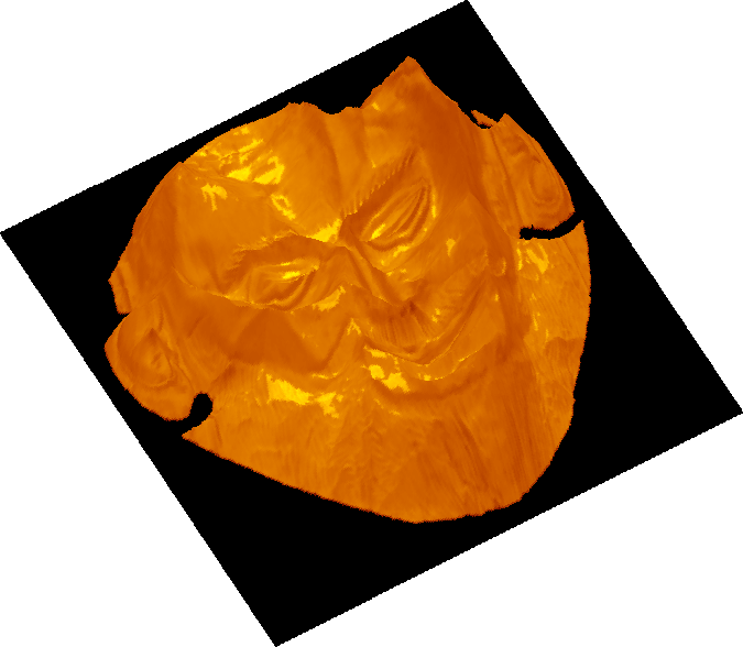
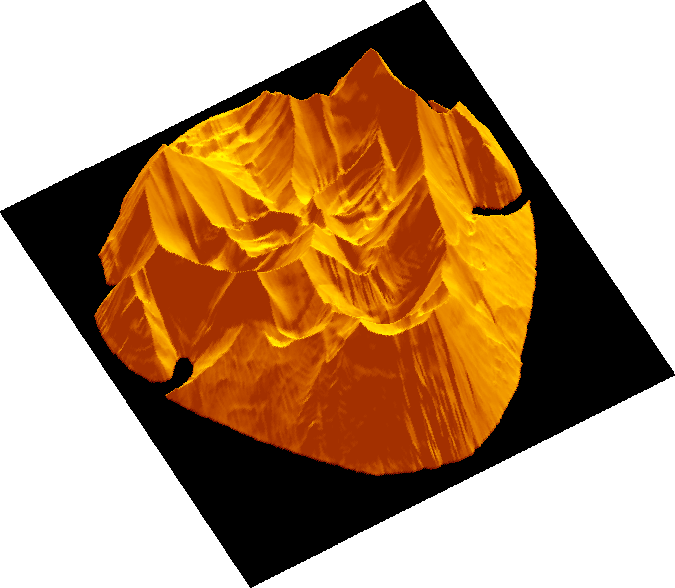
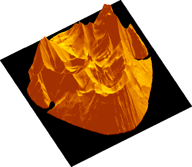
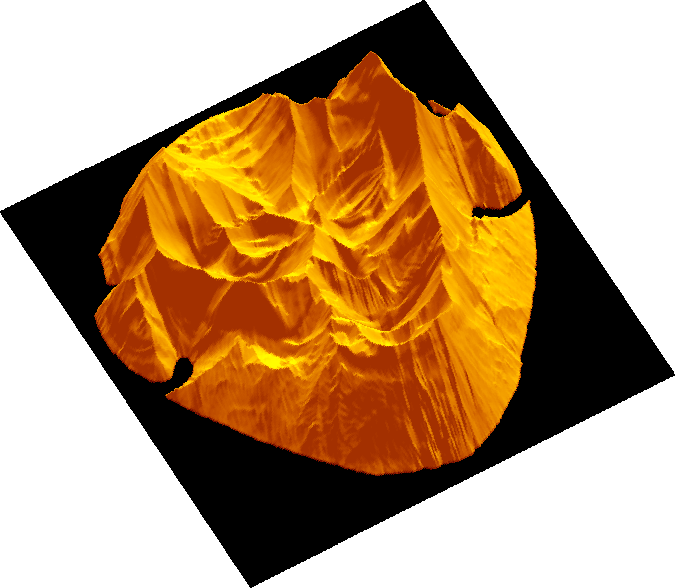
In Fig. 15 we can see the output image and the 3D reconstruction in a single case for each models. What we can note is that also using more realistic illumination models as the two non-Lambertian considered, we do not obtain a so better approximation of the ground truth solution. This is due to the missing important informations (e.g. the correct oblique light source direction, the values of the parameter involved that are known for the models but not available in the real cases) and also due to the fact that we are using a first order method of approximation.

LAM	ON4	PH4

Figure 15: Agamennon mask: results with oblique light source $\boldsymbol{\omega}_{obl}=(0,0.0995,0.9950)$. On the first row the output images, on the second row the 3D reconstruction with vertical view, on the third row the 3D reconstruction with oblique view.

Test 8: Real Vase.

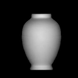
With this test we want to investigate the stability of our method with respect to the presence of noise. In fact, looking at the Fig. 16(a) we can consider that RV is a noisy version of the synthetic vase used in the Tests 5 and 6.

(a) Real Vase Input

(b) Real Vase Mask

Figure 16: Real Vase images (size $256\times 256$): (a) Input image; (b) Mask.

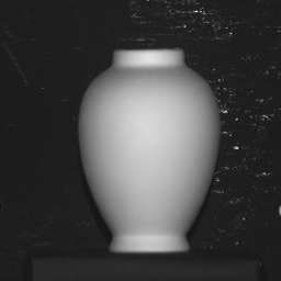
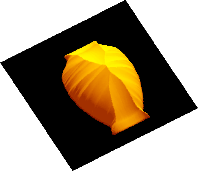
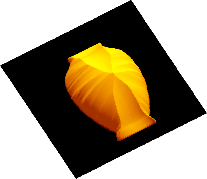
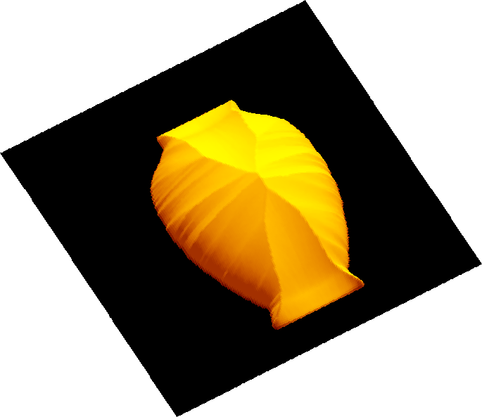
The test was performed using a vertical light source $\omega=(0,0,1)$. The output images, computed a posteriori by using the gradient of $u$ approximated via centered finite differences starting from the values of $u$ just computed by the numerical scheme, are visible in Fig. 17, first column. The reconstruction obtained with the three models are visible in the same Fig. 17, second column. What we can note is that all the reconstructions, obtained using homogeneous Dirichlet BC, suffer for a concave/convex ambiguity, as already noted for the synthetic vase (SV in the following).

Out	3D reconstruction

Figure 17: Real Vase: Output images and 3D reconstructions. On the first row the L–model, on the second row the ON–model with $\sigma=0.2$, on the third row the PH–model with $k_{S}=0.2$.

Since it is visible looking at the SV and the RV tests that we obtain results with errors of the same order of magnitude around $10^{-2}$, considering that RV is a noisy version of SV, this shows that the method is stable in the presence of noise in the image.

Table 19: Real Vase: $L^{2}$, $L^{\infty}$ errors with vertical light source $\boldsymbol{\omega}=(0,0,1)$.

SL–Schemes	$L^{2}(I)$	$L^{\infty}(I)$
LAM	0.0093	0.0784
ON-02	0.0094	0.0784
ON-04	0.0111	0.0824
PH-s02	0.0095	0.0824
PH-s04	0.0098	0.0824

Finally, in Fig. 18 one can note the behavior of the ON–model by varying the value of the parameter $\sigma$. Since in real situations we do not know it (as other parameters like the light source direction) we can only vary it in order to see the one which gives the best fit with the image. Looking at Fig. 18 what we can observe is that increasing the value of $\sigma$ the reconstruction shows a wider concave/convex ambiguity, which affects more pixels. But this holds only in this specific case, not in general for all the real images as a rule.

ON $\sigma=0.2$	ON $\sigma=0.4$	ON $\sigma=0.6$

Figure 18: Real Vase: 3D reconstructions related to the ON–model, varying $\sigma$. From left to right $\sigma=0.2,0.4,0.6$.

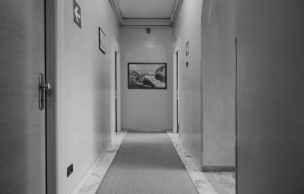
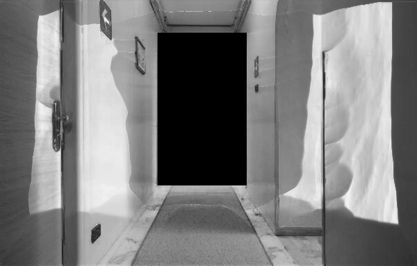
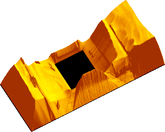
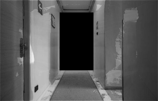
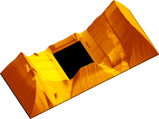
Test 9: Corridor.

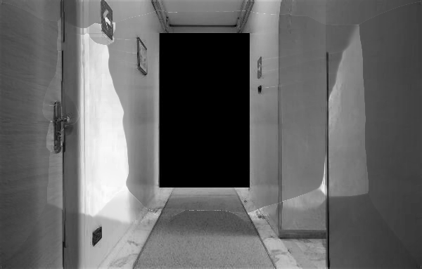
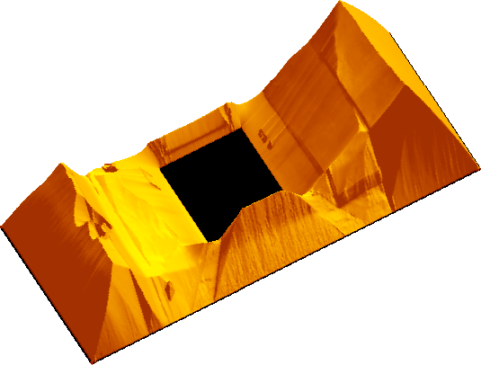
As illustrative example, let us consider a real image of a corridor (see Fig. 19) as a typical example of a scene which can be useful for a robot navigation problem. The test has been added as illustrative example to show that even for a real scene which does not satisfies all the assumptions and for which several informations are missing (e.g. boundary conditions) the method is able to compute a reasonable accurate reconstruction in the central part of the corridor (clearly the boundaries are wrong due to a lack of information). The size of this image is $600\times 383$. Note that for this picture we do not know the parameters and the light direction in the scene. It seems that there is a diffused light and more than one light source. So this picture does not satisfy many assumptions we used in the theoretical part. In order to apply our numerical scheme we considered a Dirichlet boundary condition equal to zero at the wall located at the bottom of the corridor. In this way we have a better perception of the depth of the scene. In Fig. 20 we can see the output images (on the first column) and the 3D reconstructions (on the second column) obtained by L–model, ON–model with $\sigma=0.1$ and PH–model with $k_{S}=0.2$. In this example the PH–model seems to recognize the scene better than the ON–model. In some sense this is probably due to the fact that it has less parameters so it is easier to tune to a real situation where the information on the parameters is not available. We point out that this test is just an illustration of the fact that coupling SfS with additional informations (e.g. coming from distance sensors to fix boundary conditions) can be useful to describe a scene.

Figure 19: Image of a real scene (size $600\times 383$).

Out	3D reconstruction

Figure 20: Output images and 3D reconstructions of a scene for a robot path planning application. On the first row the L–model, on the second row the ON–model with $\sigma=0.1$, on the third row the PH–model with $k_{S}=0.2$.

Test 10: Other tests on real images.

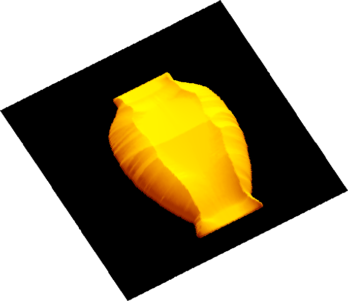
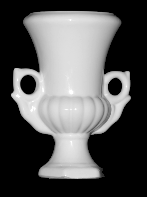
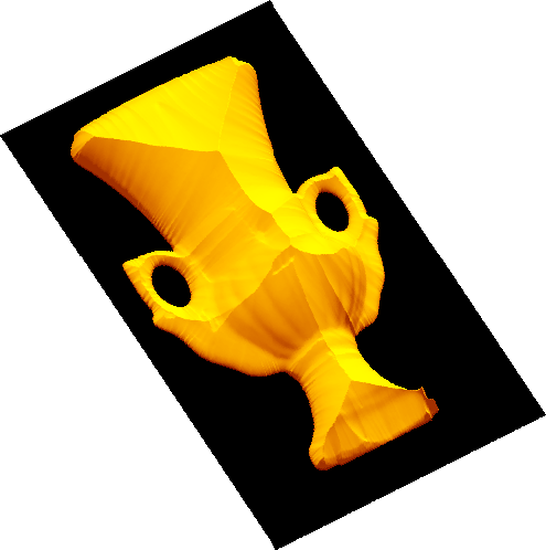
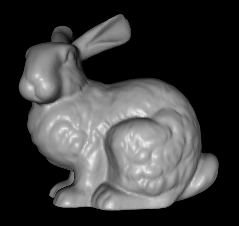
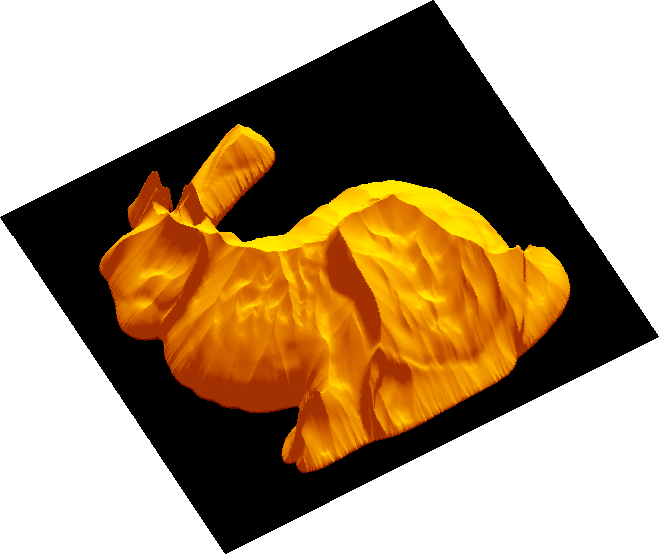
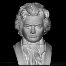
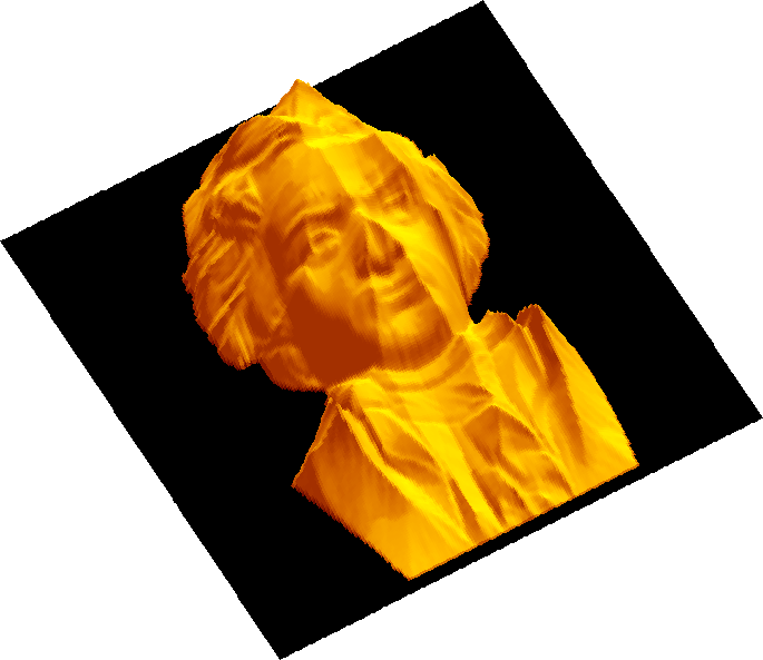
In order to demonstrate the applicability of our proposed approach for real data, we added here other experiments conducted on a real urn, real rabbit and real Beethoven’s bust. The input images and the related recovered shapes obtained by the three models studied under different light directions and parameters are shown in Fig. 21. As visible from Fig. 21, the results are quite good, even for pictures like the rabbit or the bust of Beethoven, which have many details, even if they still suffer for the concave/convex ambiguity typical of the SfS problem.

Input	reconstruction

Figure 21: Experiments on real images: input images and the recovered shapes obtained by our approach. On the first row: urn reconstructed by the L–model with $\boldsymbol{\omega}=(0,0,1)$. On the second row: rabbit reconstructed by the ON–model with $\sigma=0.2$, $\boldsymbol{\omega}=(0,0,1)$, $\mathbf{V}=(0,0,1)$. On the third row: Beethoven reconstructed by the PH–model with $\boldsymbol{\omega}=(0.0168,1.198,0.9801)$, $k_{S}=0.2$.

8 Conclusions

In this paper we derived nonlinear partial differential equations of first order, i.e. Hamilton-Jacobi equations, associated to the non-Lambertian reflectance models ON–model and PH–model. We have obtained the model equations for all the possible cases, coupling vertical or oblique light source with vertical or oblique position of the observer. This exhaustive description has shown that these models lead to stationary Hamilton-Jacobi equations with a same structure and this allows for a unified mathematical formulation in terms of fixed point problem. This general formulation is interesting because we can switch on and off the different terms related to ambient, diffuse and specular reflection in a very simple way. As a result, this general model is very flexible to treat the various situations with vertical and oblique light sources. Unfortunately, we have observed that none of these models is able to overcome the typical concave/convex ambiguity known for the classical Lambertian model. Despite this limitations, the approach presented in this paper is able to improve the Lambertian model that is not suitable to deal with realistic images coming from medical or security application. The numerical methods presented here can be applied to solve the equations corresponding to the ON–model and the PH–model in all the situations although they suffer for the presence of several parameters related to the roughness or to the specular effect. Nonetheless, looking at the comparisons with other methods or models shown in this paper, one can see that the Semi-Lagrangian approach is competitive with respect to other techniques used, both in terms of CPU time and accuracy. As we have seen, in the complex nonlinear PDEs associated to non-Lambertian models the parameters play a crucial role to obtain accurate results. In fact, varying the value of the parameters it is possible to improve the approximation with respect to the classical L–model. We can also say that for real images the PH–model seems easier to tune, perhaps because we need to manage less parameters.
Focusing the attention on the tests performed with an oblique light source, we have to do some comments that are common to the PH–model and the ON–model. Several terms appear in these models and each of them gives a contribution to the roundoff error. Note that the accumulation of these roundoff errors makes difficult in the oblique case to obtain a great accuracy. A possible improvement could be the use of second order schemes, that release the link between the space and the time steps which characterizes and limits the accuracy for first order schemes. Another interesting direction would be to extend this formulation to other reflectance models (like e.g. the Ward’s model) and/or to consider perspective projection also including an attenuation term which can help to resolve the concave/convex ambiguity or considering more than one input image with non-Lambertian models, that solves the well-known ambiguity (see [74] for a first step in this last direction considering the Blinn-Phong model). These directions will be explored in future works.

Acknowledgements

The first author wishes to acknowledge the support obtained by the INDAM under the GNCS research project ”Metodi ad alta risoluzione per problemi evolutivi fortemente nonlineari” and the hospitality obtained by Prof. Edwin Hancock of the University of York, Department of Computer Science, during her scholarship “Borsa di perfezionamento all’estero” paid by Sapienza - Università di Roma.

References

- [1] A. H. Ahmed and A. A. Farag. Shape from Shading under various imaging conditions. In IEEE International Conference on Computer Vision and Pattern Recognition CVPR’07, pages X1–X8, Minneapolis, MN, June 2007.
- [2] A.H. Ahmed and A.A. Farag. A new formulation for Shape from Shading for non-Lambertian surfaces. In Proc. IEEE Conference on Computer Vision and Pattern Recognition (CVPR), pages 1817–1824, 2006.
- [3] S. Bakshi and Y.-H. Yang. Shape-from-Shading for non-Lambertian surfaces. In Proc. IEEE International Conference on Image Processing (ICIP), pages 130–134, 1994.
- [4] G. Barles. Solutions de viscosité des équations de Hamilton-Jacobi. Springer Verlag, 1994.
- [5] S. Biswas, G. Aggarwal, and R. Chellappa. Robust estimation of albedo for illumination-invariant matching and shape recovery. Pattern Analysis and Machine Intelligence, IEEE Transactions on, 31(5):884–899, May 2009.
- [6] M.J. Brooks, W. Chojnacki, and R. Kozera. Impossible and ambiguous shading patterns. International Journal of Computer Vision, 7(2):119–126, 1992.
- [7] M.J. Brooks and B.K.P. Horn. Shape and source from shading. In Proceedings of the Ninth International Joint Conference on Artificial Intelligence (vol. II), pages 932–936, Los Angeles, CA, USA, 1985.
- [8] A. Bruss. The image irradiance equation: Its solution and application. Technical report ai-tr-623, Massachusetts Institute of Technology, June 1981.
- [9] F. Camilli and M. Falcone. An approximation scheme for the maximal solution of the Shape from Shading model. In Proceedings of the IEEE International Conference on Image Processing (vol. I), volume 1, pages 49–52, Lausanne, Switzerland, Sep 1996.
- [10] F. Camilli and L. Grüne. Numerical approximation of the maximal solutions for a class of degenerate Hamilton-Jacobi equations. SIAM Journal on Numerical Analysis, 38(5):1540–1560, 2000.
- [11] F. Camilli and A. Siconolfi. Maximal subsolutions of a class of degenerate Hamilton-Jacobi problems. Indiana University Mathematics Journal, 48(3):1111–1131, 1999.
- [12] E. Carlini, M. Falcone, and A. Festa. A brief survey on semi-lagrangian schemes for image processing. In Michael Breuss, Alfred Bruckstein, and Petros Maragos, editors, Innovations for Shape Analysis: Models and Algorithms, pages 191–218. Ed. Springer, 2013. ISBN: 978-3-642-34140-3.
- [13] A. Chambolle. A uniqueness result in the theory of stereo vision: coupling Shape from Shading and binocular information allows unambiguous depth reconstruction. Annales de l’Istitute Henri Poincarè, 11(1):1–16, 1994.
- [14] F. Courteille, A. Crouzil, J.-D. Durou, and P. Gurdjos. Towards Shape from Shading under realistic photographic conditions. In Proc. of the 17th International Conference on Pattern Recognition, volume 2, pages 277–280. Cambridge, UK, 2004.
- [15] F. Courteille, A. Crouzil, J.-D. Durou, and P. Gurdjos. Shape from shading for the digitization of curved documents. Machine Vision and Applications, 18(5):301–316, 2007.
- [16] P. Daniel and J.-D. Durou. From deterministic to stochastic methods for Shape from Shading. In Proceedings of the Fourth Asian Conference on Computer Vision, pages 187–192, Taipei, Taiwan, 2000.
- [17] J. Van Diggelen. A photometric investigation of the slopes and heights of the ranges of hills in the maria of the moon. Bulletin of the Astronomical Institute of the Netherlands, 11(423):283–290, 1951.
- [18] J.-D. Durou, J.-F. Aujol, and F. Courteille. Integrating the normal field of a surface in the presence of discontinuities. In Energy Minimization Methods in Computer Vision and Pattern Recognition (EMMCVPR), volume 5681, pages 261–273, 2009.
- [19] J.-D. Durou, M. Falcone, and M. Sagona. Numerical methods for Shape from Shading: a new survey with benchmarks computer vision and image understanding. Elsevier, 109(1):22–43, 2008.
- [20] M. Falcone. Numerical solution of Dynamic Programming equations. In Bardi, M., Dolcetta, I.C., Optimal control and viscosity solutions of Hamilton-Jacobi-Bellman equations, pages 471–504, 1997.
- [21] M. Falcone and R. Ferretti. Semi-Lagrangian Approximation Schemes for Linear and Hamilton-Jacobi Equations. SIAM, 2014.
- [22] M. Falcone and M. Sagona. An algorithm for the global solution of the Shape from Shading model. In Proceedings of the Ninth International Conference on Image Analysis and Processing (vol. I), vol. 1310 of Lecture Notes in Computer Science, pages 596–603, Florence, Italy, 1997.
- [23] M. Falcone, M. Sagona, and A. Seghini. A scheme for the Shape–from–Shading model with “black shadows”. Numerical Mathematics and Advanced Applications, pages 503–512, 2003.
- [24] H. Fassold, R. Danzl, K. Schindler, and H. Bischof. Reconstruction of archaeological finds using shape from stereo and shape from shading. In Proc. 9th Computer Vision Winter Workshop, Piran, Slovenia, pages 21–30, 2004.
- [25] P. Favaro and T. Papadhimitri. A closed-form solution to uncalibrated photometric stereo via diffuse maxima. In Proceedings of the IEEE Conference on Computer Vision and Pattern Recognition, pages 821–828, 2012.
- [26] R.T. Frankot and R. Chellappa. A method for enforcing integrability in Shape from Shading algorithms. IEEE Transactions on Pattern Analysis and Machine Intelligence, 10(4):439–451, 1988.
- [27] A. Grumpe, F. Belkhir, and C. Wöhler. Construction of lunar DEMs based on reflectance modelling. Advances in Space Research, 53(12):1735 –1767, 2014.
- [28] B.K.P. Horn. Shape from Shading: A Method for Obtaining the Shape of a Smooth Opaque Object From One View. PhD thesis, Massachusetts Institute of Technology, 1970.
- [29] B.K.P. Horn. Obtaining Shape from Shading information. In P.H. Winston (Ed.), editor, The Psychology of Computer Vision, chapter 4, pages 115–155. McGraw-Hill, 1975.
- [30] B.K.P. Horn and M.J. Brooks. The variational approach to Shape from Shading. Computer Vision, Graphics and Image Processing, 33(2):174–208, 1986.
- [31] B.K.P. Horn and M.J. Brooks. Shape from Shading (Artificial Intelligence). The MIT Press, 1989.
- [32] Katsushi Ikeuchi and Berthold K.P. Horn. Numerical Shape from Shading and occluding boundaries. Artificial Intelligence, 17(1–3):141–184, 1981.
- [33] H. Ishii and M. Ramaswamy. Uniqueness results for a class of Hamilton-Jacobi equations with singular coefficients. Communications in Partial Differential Equations, 20:2187–2213, 1995.
- [34] Y.-C. Ju, M. Breuß, A. Bruhn, and S. Galliani. Shape from Shading for rough surfaces: Analysis of the Oren-Nayar model. In Proc. British Machine Vision Conference (BMVC), pages 104.1–104.11. BMVA Press, 2012.
- [35] Y.-C. Ju, S. Tozza, M. Breuß, A. Bruhn, and A. Kleefeld. Generalised Perspective Shape from Shading with Oren-Nayar Reflectance. In Proceedings of the 24th British Machine Vision Conference (BMVC 2013), pages 42.1–42.11, Bristol, UK, 2013. BMVA Press.
- [36] J. Kain and D.N. Ostrov. Numerical Shape from Shading for discontinuous photographic images. International Journal of Computer Vision, 44(3):163–173, 2001.
- [37] R. Kozera. Existence and uniqueness in photometric stereo. Appl. Math. Comput., 44(1):103, 1991.
- [38] R. Kozera. Uniqueness in Shape from Shading revisited. Journal of Mathematical Imaging and Vision, 7(2):123–138, 1997.
- [39] S. N. Kruzkov. The generalized solution of the hamilton-jacobi equations of eikonal type i. Math. USSR Sbornik, 27:406–446, 1975.
- [40] P.L. Lions, E. Rouy, and A. Tourin. Shape-from-Shading, viscosity solutions and edges. Numerische Mathematik, 64(3):323–353, 1993.
- [41] V. Lohse, C. Heipke, and R. L. Kirk. Derivation of planetary topography using multi-image shape-from-shading. Planetary and Space Science, 54(7):661–674, 2006.
- [42] R. Mecca and M. Falcone. Uniqueness and approximation of a photometric Shape-from-Shading model. SIAM J. Imaging Sciences, 6(1):616–659, 2013.
- [43] R. Mecca and S. Tozza. Shape reconstruction of symmetric surfaces using photometric stereo. In Michael Breuss, Alfred Bruckstein, and Petros Maragos, editors, Innovations for Shape Analysis: Models and Algorithms, pages 219–243. Ed. Springer, 2013. ISBN: 978-3-642-34140-3.
- [44] T. Okatani and K. Deguchi. Shape reconstruction from an endoscope image by Shape from Shading technique for a point light source at the projection center. Computer Vision and Image Understanding, 66(2):119–131, 1997.
- [45] J. Oliensis. Shape from Shading as a partially well-constrained problem. Computer Vision, Graphics and Image Processing: Image Understanding, 54(2):163–183, 1991.
- [46] J. Oliensis. Uniqueness in Shape from Shading. International Journal of Computer Vision, 6(2):75–104, 1991.
- [47] M. Oren and S.K. Nayar. Diffuse reflectance from rough surfaces. In Proc. IEEE Conference on Computer Vision and Pattern Recognition (CVPR), pages 763–764, 1993.
- [48] M. Oren and S.K. Nayar. Generalization of Lambert’s reflectance model. In Proc. International Conference and Exhibition on Computer Graphics and Interactive Techniques (SIGGRAPH), pages 239–246, 1994.
- [49] M. Oren and S.K. Nayar. Seeing beyond Lambert’s law. In Proc. European Conference on Computer Vision (ECCV), pages 269–280, 1994.
- [50] M. Oren and S.K. Nayar. Generalization of the Lambertian model and implications for machine vision. International Journal of Computer Vision, 14(3):227–251, 1995.
- [51] B. T. Phong. Illumination for computer generated pictures. Communications of the ACM, 18(6):311–317, 1975.
- [52] E. Prados, F. Camilli, and O. Faugeras. A viscosity solution method for Shape-from-Shading without image boundary data. ESAIM: Mathematical Modelling and Numerical Analysis, 40(2):393–412, 2006.
- [53] E. Prados and O. Faugeras. A mathematical and algorithmic study of the lambertian sfs problem for orthographic and pinhole cameras. Rapport de recherche 5005, Institut National de Recherche en Informatique et en Automatique, Sophia Antipolis, France, November 2003.
- [54] E. Prados and O. Faugeras. Perspective Shape from Shading and viscosity solutions. In Proc. IEEE International Conference on Computer Vision (ICCV), pages 826–831, 2003.
- [55] E. Prados and O. Faugeras. Shape from Shading: a well-posed problem? In Proc. IEEE Conference on Computer Vision and Pattern Recognition (CVPR), volume 2, pages 870–877, 2005.
- [56] E. Prados, O. Faugeras, and E. Rouy. Shape from Shading and viscosity solutions. In Anders Heyden, Gunnar Sparr, Mads Nielsen, and Peter Johansen, editors, Computer Vision ’ ECCV 2002, volume 2351 of Lecture Notes in Computer Science, pages 790–804. Springer Berlin Heidelberg, 2002.
- [57] Y. Quéau, F. Lauze, and J.-D. Durou. Solving uncalibrated photometric stereo using total variation. Journal of Mathematical Imaging and Vision, 52(1):87–107, 2015.
- [58] H. Ragheb and E.R. Hancock. Surface normals and height from non-lambertian image data. In Proc. International Symposium on 3D Data Processing, Visualization and Transmission (3DPVT), pages 18–25, 2004.
- [59] H. Ragheb and E.R. Hancock. Surface radiance correction for Shape from Shading. Pattern Recognition, 38(10):1574–1595, 2005.
- [60] T. Rindfleisch. Photometric method for lunar topography. Photogrammetric Engineering, 32(2):262–277, 1966.
- [61] E. Rouy and A. Tourin. A viscosity solutions approach to Shape-from-Shading. SIAM Journal on Numerical Analysis, 29(3):867–884, June 1992.
- [62] M. Sagona. Numerical methods for degenerate Eikonal type equations and applications. PhD thesis, Dipartimento di Matematica dell’Università di Napoli ””Federico II”, Napoli, Italy, November 2001.
- [63] D. Samaras and D. Metaxas. Incorporating illumination constraints in deformable models for Shape from Shading and light direction estimation. IEEE Transactions on Pattern Analysis and Machine Intelligence, 25(2):247–264, 2003.
- [64] W.A.P. Smith and E.R. Hancock. Recovering facial shape and albedo using a statistical model of surface normal direction. In 10th IEEE International Conference on Computer Vision (ICCV 2005), 17-20 October 2005, Beijing, China, pages 588–595, 2005.
- [65] W.A.P. Smith and E.R. Hancock. Estimating facial albedo from a single image. IJPRAI, 20(6):955–970, 2006.
- [66] W. Steffen, N. Koning, S. Wenger, C. Morisset, and M. Magnor. Shape: A 3d modeling tool for astrophysics. Visualization and Computer Graphics, IEEE Transactions on, 17(4):454–465, April 2011.
- [67] T.M. Strat. A numerical method for Shape from Shading from a single image. Master’s thesis, Department of Electrical Engineering and Computer Science, Massachussetts Institute of Technology, Cambridge, MA, USA, 1979.
- [68] R. Szeliski. Fast Shape from Shading. Computer Vision, Graphics and Image Processing: Image Understanding, 53(2):129–153, 1991.
- [69] A. Tankus and N. Kiryati. Photometric stereo under perspective projection. In Proc. IEEE International Conference on Computer Vision (ICCV), volume 1, pages 611–616, 2005.
- [70] A. Tankus, N. Sochen, and Y. Yeshurun. Shape-from-Shading Under Perspective Projection. International Journal of Computer Vision, 63(1):21–43, 2005.
- [71] S. Tozza. Analysis and Approximation of Non-Lambertian Shape-from-Shading Models. PhD thesis, Dipartimento di Matematica, Sapienza - Università di Roma, Rome, Italy, January 2015.
- [72] S. Tozza and M. Falcone. A comparison of non-lambertian models for the Shape–from-Shading problem. In Michael Breuss, Alfred Bruckstein, Petros Maragos, and Stefanie Wuhrer, editors, New Perspectives in Shape Analysis. Ed. Springer. To appear.
- [73] S. Tozza and M. Falcone. A Semi-Lagrangian Approximation of the Oren-Nayar PDE for the Orthographic Shape–from–Shading Problem. In Sebastiano Battiato and José Braz, editors, Proceedings of the 9th International Conference on Computer Vision Theory and Applications (VISAPP), volume 3, pages 711–716. SciTePress, 2014.
- [74] S. Tozza, R. Mecca, M. Duocastella, and A. Del Bue. Direct differential Photometric-Stereo shape recovery of diffuse and specular surfaces. International Journal of Mathematical Imaging and Vision (JMIV). To appear.
- [75] O. Vogel, M. Breuß, T. Leichtweis, and J. Weickert. Fast Shape from Shading for phong-type surfaces. In Xue-Cheng Tai, Knut Mørken, Marius Lysaker, and Knut-Andreas Lie, editors, Scale Space and Variational Methods in Computer Vision, volume 5567 of Lecture Notes in Computer Science, pages 733–744. Springer, 2009.
- [76] O. Vogel, M. Breuß, and J. Weickert. Perspective Shape from Shading with non-Lambertian reflectance. In Proc. DAGM Symposium on Pattern Recognition, pages 517–526, 2008.
- [77] O. Vogel, L. Valgaerts, M. Breuß, and J. Weickert. Making shape from shading work for real-world images. In Joachim Denzler, Gunther Notni, and Herbert Süße, editors, Pattern Recognition, volume 5748 of Lecture Notes in Computer Science, pages 191–200. Springer Berlin Heidelberg, 2009.
- [78] Wikipedia. Mask of Agamemnon. Website. http://en.wikipedia.org/wiki/Mask_of_Agamemnon.
- [79] Lawrence B. Wolff, Shree K. Nayar, and Michael Oren. Improved diffuse reflection models for computer vision. International Journal of Computer Vision, 30(1):55–71, 1998.
- [80] L.B. Wolff. Diffuse-reflectance model for smooth dielectric surfaces. Journal of the Optical Society of America A, 11(11):2956–2968, 1994.
- [81] R. J. Woodham. Photometric method for determining surface orientation from multiple images. Optical Engineering, 19(1):134–144, 1980.
- [82] P.L. Worthington and E.R. Hancock. New constraints on data-closeness and needle map consistency for Shape-from-Shading. IEEE Transactions on Pattern Analysis and Machine Intelligence, 21(12):1250–1267, 1999.
- [83] C. Wu, S. Narasimhan, and B. Jaramaz. A multi-image Shape-from-Shading framework for near-lighting perspective endoscopes. International Journal of Computer Vision, 86:211–228, 2010.
- [84] K.-J. Yoon, E. Prados, and P. Sturm. Joint estimation of shape and reflectance using multiple images with known illumination conditions. International Journal of Computer Vision, 86:192–210, 2010.
- [85] R. Zhang, P.-S. Tsai, J.E. Cryer, and M. Shah. Shape from Shading: a survey. IEEE Transactions on Pattern Analysis and Machine Intelligence, 21(8):690–706, 1999.
- [86] Qinfen Zheng and R. Chellappa. Estimation of illuminant direction, albedo, and shape from shading. In Computer Vision and Pattern Recognition, 1991. Proceedings CVPR ’91., IEEE Computer Society Conference on, pages 540–545, Jun 1991.