A stable finite-difference scheme for growth and diffusion on a map

Abstract

We describe a general Godunov-type splitting for numerical simulations of the Fisher–Kolmogorov–Petrovski–Piskunov growth and diffusion equation in two spatial dimensions. In particular, the method is appropriate for modeling population growth and dispersal on a terrestrial map. The procedure is semi-implicit, hence quite stable, and approximately $O(\Delta x^{2})+O(\Delta t^{2})$ accurate, excluding boundary condition complications. It also has low memory requirements and shows good performance. We illustrate an application of this solver: global human dispersal in the late Pleistocene, modeled via growth and diffusion over geographical maps of paleovegetation and paleoclimate.

Keywords: reaction-diffusion equations , finite-difference solvers, population dynamics

1 Introduction

There is an increasing interest in modeling population dynamics at large spatial and temporal scales, for example the modern human out-of-Africa dispersal (Eriksson et al., 2012; Henn et al., 2012; Nikitas and Nikita, 2005; Young and Bettinger, 1995) or Neanderthal dispersal and extinction (Callegari et al., 2013). These models are required to interpret local and global patterns of genetic, phenetic and cultural variation (Bouckaert et al., 2012; Eriksson et al., 2012; Manica et al., 2007; Pinhasi et al., 2005; Relethford, 2004).

Fisher (Fisher, 1937) studied the description – via a reaction-diffusion equation – of an analogous but one-dimensional problem: the propagation of an advantageous genetic mutation within an already-present population, situated along a coast line. Kolmogorov, Petrovskii and Piskunov (Kolmogorov et al., 1937) were more general; in particular, their analysis treated the two-dimensional case. Such a model (called Fisher/KPP in the following) was first applied to the dispersal and growth of a population by Skellam (Skellam, 1951), and serves as an important control for designing and validating other more complex spatiotemporal population models (Callegari et al., 2013). Coupling population dynamics with models of large-scale changes in continental topography, climate, and ecosystem productivity is essential to understand the role of environmental constraints on patterns of genetic, phenetic, and cultural variation among human populations (Callegari et al., 2013).

Here we present a stable and efficient finite-difference solver for the Fisher/ KPP equation on 2-D domains of arbitrary shape (e.g. geographical maps), and show how it can be extended to include environmental fluctuations. In a brief outline of our paper, we will: review the derivation of the Fisher/KPP equation (Section 2); develop finite-difference schemes in 1 and 2 dimensions for constant environmental carrying capacity, $\mathcal{K}$ (Section 3); extend the scheme to allow for space- and time-dependent $\mathcal{K}(\mathbf{x},t)$ (Section 4) and irregular domains such as geographical maps; show an application of this technique to the out-of-Africa dispersal of Homo sapiens by using net primal productivity (NPP) as a proxy for $\mathcal{K}(\mathbf{x},t)$ (Section 5).

2 The Fisher/KPP equation

An intuitive way to get the Fisher/KPP equation (Fisher, 1937; Kolmogorov et al., 1937; Skellam, 1951) is as follows. A current $\mathbf{j}$ of particles (e.g., individuals) moving across an interface located at $\mathbf{x}$ is proportional to the gradient of the population density $p$ (“Fickian diffusion”)

$$\mathbf{j}=-c\,\nabla p.$$

The rate of change of $p$ is then given by the mass balance equation (Reichl, 2004), which for Fickian diffusion reads

$$\frac{\partial p}{\partial t}-c\,\nabla^{2}p=\rho.$$

If $\rho=0$, this is the heat equation when $c=\mathcal{D}/2$ and $\mathcal{D}$ is the diffusion coefficient. For lack of a better model, we assume $c$ is a constant (Young & Bettinger (Young and Bettinger, 1995)). The source term $\rho$ is usually modeled by a logistic growth function, $\rho=\lambda p(1-p/\mathcal{K})$, yielding the Fisher/KPP equation

$$\frac{\partial p}{\partial t}=\lambda\left(1-\frac{p}{\mathcal{K}}\right)p+c\,\nabla^{2}p,$$ (1)

where $\mathcal{K}$ is called carrying capacity and $\lambda$ is the growth rate. In (1) we assumed $\mathcal{K}$ is constant, but it suffices that there is an upper limit $\bar{\mathcal{K}}$, in which case $0\leq p/\bar{\mathcal{K}}\leq 1$. This scaled version will be used in (2) below. Fisher and KPP were particularly interested in the traveling wave case, $p(t,\mathbf{x})=f(\mathbf{x}_{0}+\mathbf{v}t)$. Notice what happens here if $f$ exists:

$$\mathbf{v}\cdot\nabla f=\lambda\left(1-\frac{f}{\mathcal{K}}\right)f+c\,\nabla^{2}f,$$

which in 1-D becomes a second order ordinary differential equation

$$v\frac{{\rm d}f}{{\rm d}x}=\lambda\left(1-\frac{f}{\mathcal{K}}\right)f+c\frac{{\rm d}^{2}f}{{\rm d}x^{2}}.$$

If $v$ were known, this ODE could be solved using pvp4c from MatLab, for example. By the rescalings show in Table 1, for constant $\mathcal{K}$ the Fisher/KPP equation (1) will be used in the form

$$\frac{\partial u}{\partial t}=(1-u)u+\frac{1}{2}\,\nabla^{2}u,$$ (2)

where the only sensible solutions have $0\leq u\leq 1$. The initial distribution $u(0,\mathbf{x})=u_{0}(\mathbf{x})$ must be defined for all $\mathbf{x}$.

Table 1: Variables in left column are scaled versions of those in right column.

In (2)	In (1)
$\mathbf{x}$	$\sqrt{\frac{\lambda}{2c}}\,\mathbf{x}$
$t$	$\lambda t$
$u$	$p/\mathcal{K}$

In Murray ((Murray, 2002), eq. (11.17)) our growth coefficient $\lambda$ is called $r$ and $c$ is denoted by $D$, whereas in Young and Bettinger (Young and Bettinger, 1995) the growth coefficient is $R$ and the diffusion coefficient is $K$. These inputs to our code are given in units of yr^-1 and km²/yr respectively.

3 Numerical methods and splitting

In one dimension, (2) can be solved using the MatLab function pdepe. In fact, if the system is two-dimensional but rotationally symmetric, pdepe can again be used with the radial part of the Laplace operator in cylindrical coordinates,

$$\nabla^{2}=\frac{1}{r}\frac{\partial}{\partial r}r\frac{\partial}{\partial r}+\mbox{non-contributing terms},$$

requiring only that one sets a pdepe parameter m=1. Although the MatLab function pdepe is robust, it cannot be generalized to arbitrary 2-D domains. However, it is a valuable control for testing more general solvers, and a more general solver is what we wish to explore here.

3.1 The finite-difference scheme

Since the map on which we will be working is a pixelized plane, an obvious method uses finite differences. First, however, let us examine the 1-D case for (2). In this situation, the second order derivative becomes a differencing operator in matrix form acting on the vector $\{u_{j},j=1,n\}$, where $u_{j}=u(x_{0}+(j-1)\Delta x)$,

$$\frac{d^{2}u}{dx^{2}}\rightarrow\frac{1}{(\Delta x)^{2}}Au,$$

where the matrix $A$ is

$$A=\left(\begin{array}[]{cccccc}-2&1&0&0&\ldots&0\\ 1&-2&1&0&\ldots&0\\ 0&1&-2&1&\ldots&\\ 0&0&1&\ldots&&\\ 0&0&\ldots&0&1&-2\end{array}\right).$$ (3)

If $h$ is the time step, the Courant–-Friedrichs–-Lewy (CFL) parameter (Strang and Aarikka, 1986) is

$$k=\frac{h}{2(\Delta x)^{2}}.$$

An explicit integrator for (2) would require $k<1/4$ (LeVeque, 2007; Strang and Aarikka, 1986). In our case, because the boundary conditions are so irregular on a map, we are less interested in a method of higher order than $2nd$ because stability is more important (Godunov and Ryabenkii, 1987).

Using this notation, the lowest order approximation is Euler’s method which estimates the next step $u(t+h)$ by

$$u_{E}=u(t)+k\,Au(t)+h\,(1-u(t))u(t),$$ (4)

which should be considered a vector equation in $u(t)=\{u_{j}(t),j=1,n\}$. The logistic terms, which are diagonal, should be taken to mean $((1-u)u)_{j}=(1-u_{j})u_{j}$ for $j=1,2,\ldots,n$. Euler’s method is both low-accuracy and usually unstable if it is used alone over many steps. But, it is $O(h)$ accurate and thus useful as an explicit estimate in $O(h)$ terms. An application of the trapezoidal rule yields

$$u(t+h) = u(t)+\frac{k}{2}\left(Au(t+h)+Au(t)\right)$$

$$\qquad+\frac{h}{2}\left((1-u(t+h))u(t+h)+(1-u(t))u(t)\right)$$

and is an $O(h^{2})+O((\Delta x)^{2})$ accurate procedure but solving the quadratic vector equation (3.1) for $u(t+h)$ is awkward. To the same $O(h^{2})$, we propose a semi-implicit procedure which uses the Euler estimate (4) to replace one of the terms in (3.1):

$$u(t+h) = u(t)+\frac{k}{2}\left(Au(t+h)+Au(t)\right)$$

$$\qquad+\frac{h}{2}\left((1-u_{E})u(t+h)+(1-u(t))u(t)\right).$$

Equation (3.1) can now be solved as a linear system,

$$\left(1-\frac{k}{2}A-\frac{h}{2}(1-u_{E})\right)u(t+h)=u(t)+\frac{k}{2}Au(t)+\frac{h}{2}(1-u(t))u(t),$$ (7)

because the matrix, $1-\frac{k}{2}A-\frac{h}{2}(1-u_{E})$, on the left hand side is explicit, as is the right hand side. That is, this matrix and the right hand side contain only old data, namely only information from the previous step, $u(t)$. Euler estimate $u_{E}$ is an explicit one step computation using $u(t)$. Significant advantages are: the matrix on the left hand side is tridiagonal with constants on the sub/super-diagonals, and the diagonal terms are $O(1)$ strong. The procedure (7) is only linearly stable but we will show empirically that it gives good results when compared to pdepe when this MatLab function is appropriate, that is, in both the one-dimensional and rotationally symmetric 2-D case. Not only is the method (7) step-wise stable but also stable for initial data which may not be smooth.

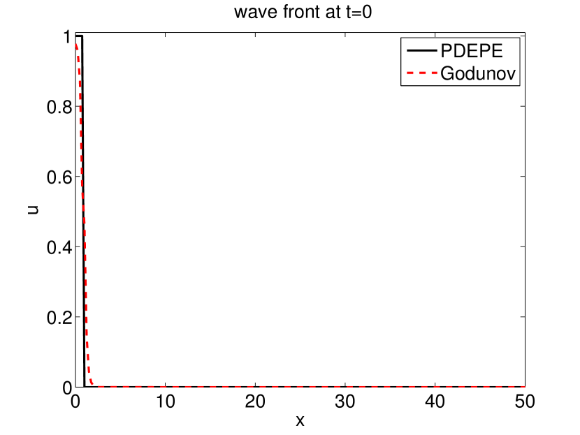
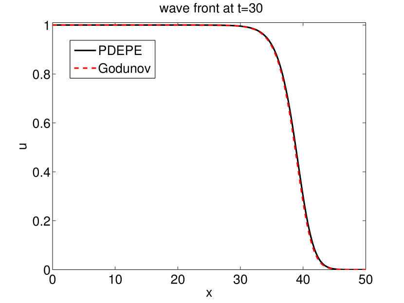
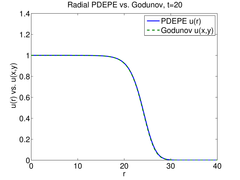
Figure 1 shows the results for $h=1/5$, $k=2.5$ compared to pdepe. Notice that at $t=20$ the agreement is remarkable; and that at $t=h$, where the wave front profile is very steep, our Godunov splitting described in Section 3.2, specifically eq.(8), is very stable. The CFL number, $k=2.5$, used to get Figure 1 is much larger than would be possible with an explicit method (LeVeque, 2007).

3.2 2-D case: Godunov–Strang–Yoshida splittings

It turns out that a generalization to the 2-D problem is a straightforward variant of Strang–Yoshida splittings (Strang, 1968; Yoshida, 1990), which are themselves variants of Godunov’s method (Godunov and Ryabenkii, 1987). The following is a fully implicit variant of our two-dimensional scheme, with two intermediate arrays, $u^{\star}$ and $u^{\star\star}$,

$$u^{\star} =u(t)+\frac{k}{4}\left(A_{x}u^{\star}+A_{x}u(t)\right)$$ (8a)

$$u^{\star\star} =u^{\star}+\frac{k}{2}\left(A_{y}u^{\star\star}+A_{y}u^{\star}\right)$$ (8b)

$$\qquad\;+\frac{h}{2}\left((1-u^{\star\star})u^{\star\star}+(1-u^{\star})u^{\star}\right)$$

$$u(t+h) =u^{\star\star}+\frac{k}{4}\left(A_{x}u(t+h)+A_{x}u^{\star\star}\right).$$ (8c)

In (8), the operators $A_{x}$ and $A_{y}$ are the same as (3) for directions $x$ and $y$, respectively. For simulations on a lattice, $u_{ij}(t)=u(t,x_{0}+(i-1)\Delta x,y_{0}+(j-1)\Delta y)$, where $1\leq i\leq N_{x},\,1\leq j\leq N_{y}$ and $\Delta x=\Delta y$, the following gives the action of the $A_{x},A_{y}$ operators:

$$A_{x}u_{i,j} = u_{i-1,j}-2u_{i,j}+u_{i+1,j},$$

$$A_{y}u_{i,j} = u_{i,j-1}-2u_{i,j}+u_{i,j+1}.$$

The compression scheme and code outline given in Appendix A show that only a maximum of one row or column (i.e., max($N_{x},N_{y})$) of storage is needed for $u^{\star}$ and $u^{\star\star}$.

Again because the fully implicit quadratic vector equation in (8b) is awkward to solve, we use an Euler estimate in one of the terms. Here is one integration time step of (8) in discrete semi-implicit form:

$$\left(1-\frac{k}{4}A_{x}\right)u^{\star} =\left(1+\frac{k}{4}A_{x}\right)u(t)$$ (9a)

$$u_{E} =u^{\star}+kA_{y}u^{\star}+h(1-u^{\star})u^{\star}$$ (9b)

$$\left(1-\frac{k}{2}A_{y}-\frac{h}{2}(1-u_{E})\right)u^{\star\star} =\left(1+\frac{k}{2}A_{y}+\frac{h}{2}(1-u^{\star})\right)u^{\star}$$ (9c)

$$\left(1-\frac{k}{4}A_{x}\right)u(t+h) =\left(1+\frac{k}{4}A_{x}\right)u^{\star\star}.$$ (9d)

Equations (9a), (9c), and (9d) are solved in sequence as multiple independent tridiagonal systems for $u^{\star},u^{\star\star}$ and the final step $u(t+h)$.

3.3 Symmetries in 2-D case

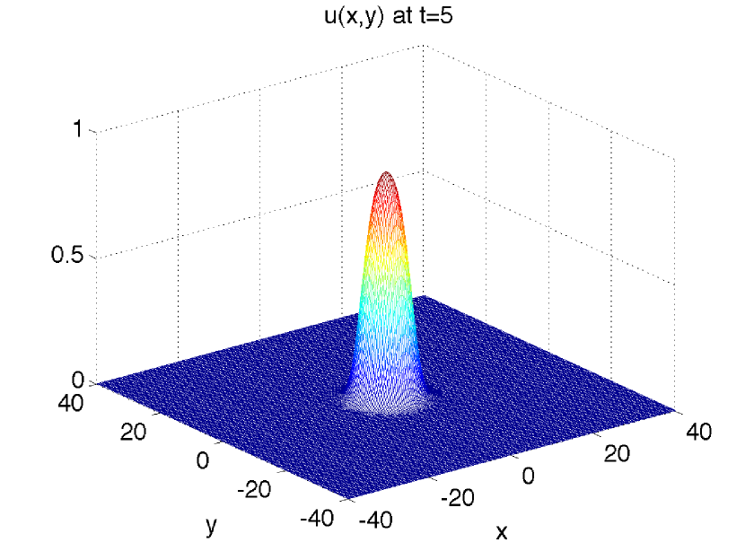
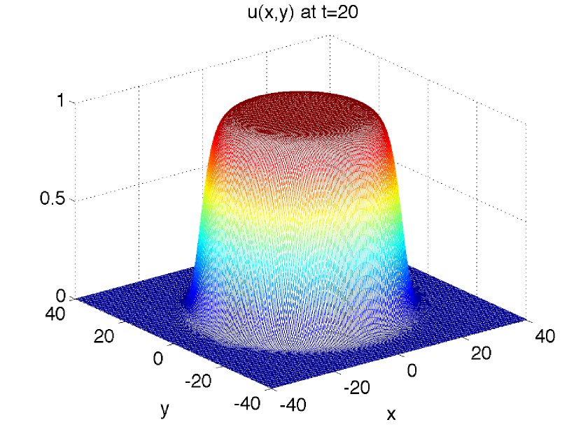
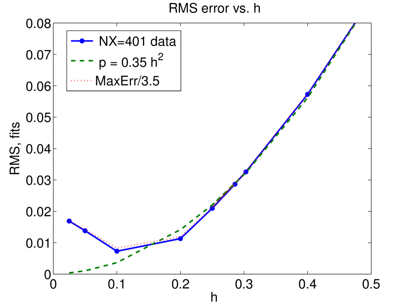
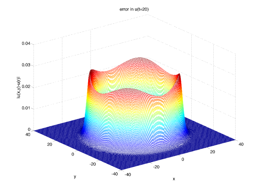
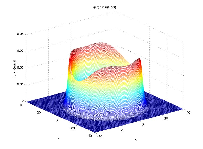
Our Godunov scheme (9) is not rotationally symmetric, and thus one way to estimate the error is to assess a solution using (9) for a symmetric problem. Again, we can use pdepe but now with the cylindrically symmetric parameter choice m=1 (see Section 12.5 in (Higham and Higham, 2005)). Figure 2 shows that any asymmetries are not apparent without more careful examination. Even the wave front portrait of the 2-D case in the left-hand panel of Figure 3 and the error estimate in the right-hand panel of the same Figure are not sufficiently quantitative. In particular, there should be no distinction between $x$ and $y$ directions in (8), while a 2-D plot of the error distribution shows a small asymmetry (compare the right-hand plot in Figure 4 to the left).

For this reason, we implemented an alternating direction method, à la Crank-Nicholson (LeVeque, 2007; Ritchmyer and Morton, 1967), which makes the error distribution more symmetric. The left panel of Figure 4 shows that, while symmetrization only slightly improves the r.m.s. and maximum errors, they have now the desirable property of being more rotationally equi-distributed: respectively, cyclic groups $C_{4}$ vs. $C_{2}$. Relatively larger deviations from the pdepe solution now correspond to directions diagonal to the spatial lattice, as expected, and do not reflect the arbitrary choice of $x$ and $y$ in the integration.

4 Fisher/KPP on maps

The next natural step when applying a reaction-diffusion equation to the modeling of population dispersal is to include geographical and environmental effects. In this Section, we discuss how to implement our solver on domains with space- and time-dependent $\mathcal{K}$, and then how to treat irregular boundaries that arise when solving Fisher/KPP on geographical maps. Using the same Godunov-type splitting described above, it is more straightforward to do the simulations on a map than might be expected.

4.1 Maps with space-dependent capacity

In our scaling of (2), the maximum population density at $\mathbf{x}$ is unity. Thus, in the following we will use a scaled carrying capacity $0<\mathcal{K}(\mathbf{x})\leq 1$. Our algorithm (8) can be modified in a straightforward way for the case that $\mathcal{K}(\mathbf{x},t)$ also depends explicitly on time: see Section 4.4. First, however, let us deal with the time independent $\mathcal{K}(\mathbf{x})$ case,

$$\frac{\partial u}{\partial t}=(1-\frac{u}{\mathcal{K}})u+\frac{1}{2}\,\nabla^{2}u,$$ (10)

(we dropped the $\mathbf{x}$ dependence of $\mathcal{K}$ for convenience of notation), for which the Godunov splitting (8) now becomes

$$\left(1-\frac{k}{4}A_{x}\right)u^{\star} =\left(1+\frac{k}{4}A_{x}\right)u(t)$$ (11a)

$$u_{E} =u^{\star}+kA_{y}u^{\star}+h(1-\frac{u^{\star}}{\mathcal{K}})u^{\star}$$ (11b)

$$\left(1-\frac{k}{2}A_{y}-\frac{h}{2}(1-\frac{u_{E}}{\mathcal{K}})\right)u^{\star\star} =\left(1+\frac{k}{2}A_{y}+\frac{h}{2}(1-\frac{u^{\star}}{\mathcal{K}})\right)u^{\star}$$ (11c)

$$\left(1-\frac{k}{4}A_{x}\right)u(t+h) =\left(1+\frac{k}{4}A_{x}\right)u^{\star\star}.$$ (11d)

Again, as in (8), multiple tridiagonal system solves must be carried out: $N_{y}$ $x$-direction solutions (11a), $N_{x}$ $y$-direction solutions (11c), and finally, another $N_{y}$ $x$-direction solutions (11d). Hopefully no confusion will result from the notation: $k$ is the CFL parameter, while $\mathcal{K}$ is the (space-dependent) carrying capacity.

4.2 A desert test of space-dependent capacity

Now we are in uncharted territory. To assess if the solver (11) works, let us examine a problem where we can compute a solution by independent means. The test setup follows below. Its motivations will be explained further in Section 4.3.

The desert test:

1. for $-y_{0}\leq y\leq y_{0}$, $\mathcal{K}=\mathcal{K}(x)$ is independent of $y$;

2. for $x_{0}\leq x\leq x_{L}$, let $\mathcal{K}=1$, while for $x_{L}<x<x_{H}$, let $\mathcal{K}=f_{r}$, where the fraction $0<f_{r}\leq 1$ defines a desert (inhospitable region) in the domain. Finally, for $x_{H}\leq x\leq x_{1}$, again set $\mathcal{K}=1$;

3. initialize $u(x,y,t=0)$ to a strip midway between $x_{0}$ and $x_{L}$, then run the simulation to study the traveling wave behavior across the $[x_{L},x_{H}]$ desert.

In other words, the variable carrying capacity domain has $\mathcal{K}=1$ for $x\leq x_{L}$ and $x\geq x_{H}$, but $\mathcal{K}=f_{r}$ in an $x$-direction desert. If the initial data $u(\mathbf{x},0)$ are widely distributed enough (nearly full $y$-width), near the middle of the domain, i.e. $y=0$, the problem looks basically one-dimensional. Thus we can again use pdepe from MatLab to compute the behavior of the one-directional wave as it passes through the desert, and compare this solution to the behavior of our Godunov method near this same center line. According to KPP (Kolmogorov et al., 1937), the velocity in the desert is the same as in the ${\mathcal{K}}=1$ region, and far enough from transients it should be approximately

$$V=\sqrt{2a},$$

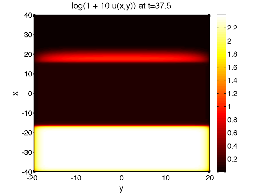
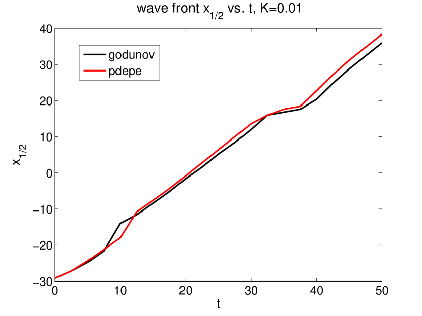
where parameter $a=\frac{{\rm d}\rho}{{\rm d}u}(u=0)$. In our case $\rho(u)=u(1-u/\mathcal{K})$, so $\frac{{\rm d}\rho}{\rm du}(0)=1$. Thus, when not entering or leaving the desert, the velocity should be $\sqrt{2}$ (Kolmogorov et al., 1937). Figure 5 shows that the velocity agrees with the KPP prediction, and is nearly constant except for short transients entering and exiting the desert, as expected. Our metric for measuring this velocity is to find, on the leading edge of the wave front, the position $x_{1/2}$ where $u(x_{1/2})=\mathcal{K}/2$.

If the jump in $\mathcal{K}$ is deep enough ($f_{r}\ll 1$), however, the integrator will fail without some regularization. The parameters for the results shown in Figure 5 are $\mathcal{K}=1$ above and below the desert, but $\mathcal{K}=0.01$ in the desert. For this case, $\frac{u}{\mathcal{K}}\gg\frac{2}{h}$ gives an instability with unpleasant sign changes, and a regularization scheme has to be used. We show this in the next subsection.

4.3 Regularization against holes and noise

An obvious problem with deep holes, jumps or ragged noise in the carrying capacity $\mathcal{K}$ is this: the right hand side of equation (11c) (as well as (16c) in the next Section) contains the term

$$\left(1+\frac{k}{2}A_{y}+\frac{h}{2}(1-\frac{u^{\star}}{\mathcal{K}})\right)u^{\star},$$ (12)

which for large ${u^{\star}}/{\mathcal{K}}$ basically determines the sign of the $u(t+h)$ on the left side of (11c) (likewise (16c)). Since both $u^{\star}$ and $\mathcal{K}$ are positive, if $\mathcal{K}$ is very small in some pixel, then we may have

$$\frac{u^{\star}}{\mathcal{K}}\gg\frac{2}{h},$$

in which case $u(t+h)$ changes sign. This is unphysical, so we would like to regularize the term (12). To do so, we need to find a monotonically increasing function, call it $g(x)$, such that

$$g(x)\sim\left\{\begin{array}[]{ll}x&\mbox{when}\,x\,\mbox{is small}\\ 1&\mbox{when}\,x\,\mbox{is large.}\end{array}\right.$$

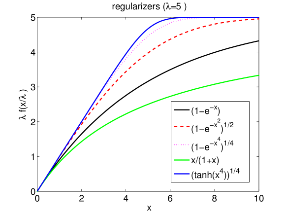
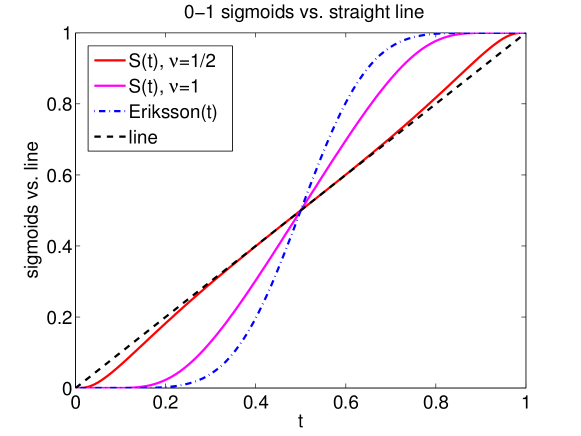
Multiple choices are available, as shown in Figure 6. We want a straight line with slope 1 when $x$ is small, then a smooth but rapid cut-off when $x=\frac{u^{\star}}{\mathcal{K}}$ gets too large. Some suitable choices are $(1-\exp{(-x^{\beta})})^{1/\beta}$, or just as cheap to compute,

$$g(x)=\left(\tanh{(x^{\beta})}\right)^{1/\beta},$$ (13)

or any variant shown in Figure 6. We choose $g(x)$ with $\beta=4$. The regularization (13) to be used in (12) and thus (11c) (likewise (16c) in the next section) is then modified to

$$\frac{u^{\star}}{\mathcal{K}}\mapsto\frac{1}{h}g(h\frac{u^{\star}}{\mathcal{K}})$$ (14)

where $h$ is the step-size. In the desert test presented above, using the regularizer yields the same results as decreasing $h$ tenfold.

One alternative to the above regularization (14) is to use smoothing by a low pass filter which weights a center pixel (map coordinate $i,j$) and its nearest $(2L-1)\times(2L-1)-1$ neighbors. A neighboring pixel with $X,Y$ distances $i_{x},j_{y}$ from $(i,j)$, has weight

$$w(i_{x},j_{y})=\left(1-(i_{x}/L)^{2}\right)\left(1-(j_{y}/L)^{2}\right)$$ (15)

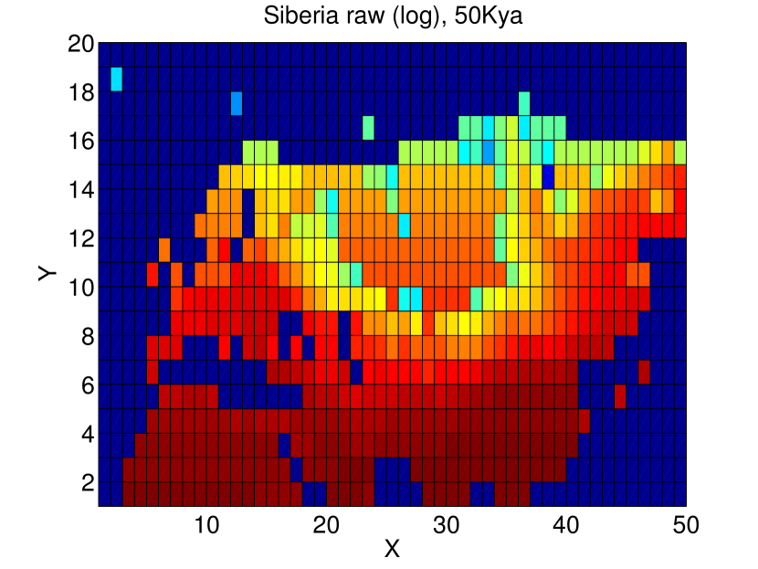
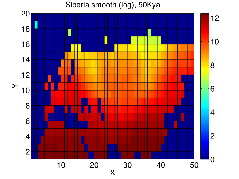
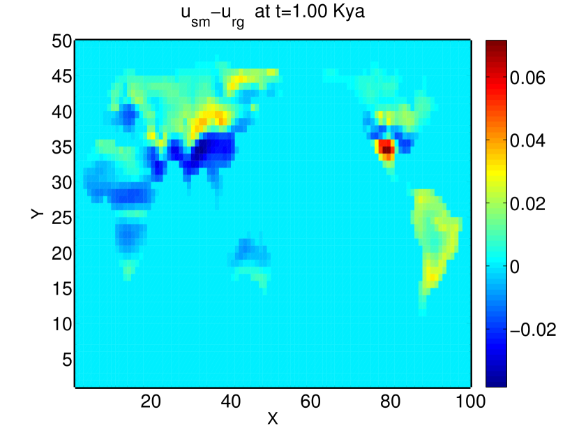
for all $-L<i_{x}<L$ and $-L<j_{y}<L$, including center at $i_{x}=j_{y}=0$. Neighboring pixels with coordinates $(i+i_{x},j+j_{x})$ having zero value (e.g. water), $i+i_{x}>{\rm N_{X}}$ or $i+i_{x}<1$, are ignored. In Mercator projection maps, $Y$ coordinates are periodic in the longitude direction). For each $(i,j)-$pixel to be smoothed, a total of each accepted (non-zero) neighbor’s weight was kept and the resulting total was normalized appropriately. The choice (15) is an approximate Gaussian weight $\exp{(-\Delta x^{2}-\Delta y^{2})}$, cut off at distances $|i_{x}|\geq L$ and $|j_{y}|\geq L$ or at uninhabitable pixels. Figure 7 shows an example of the effect of a low-pass filter (5 cells half-width, eq. (15)) smoothing on one of the maps used in this study. A comparison between regularization and smoothing is shown on the right hand plot of Figure  9.

4.4 Time-dependent capacity maps

Fluctuations in climate produce environmental changes in vegatation, sea levels, opening/closing of land bridges, waxing/waning of ice sheets, and perturbations to habitable areas in general. Thus, time-dependent environments compel us to extend our procedure (11) for both space- and time-dependent $\mathcal{K}(\mathbf{x},t)$ (see Section 5.2).

Since (11) is basically the trapezoidal method (see section 5.3 in (LeVeque, 2007)), the modification for a time-dependent $\mathcal{K}$ is as follows:

$$\left(1-\frac{k}{4}A_{x}\right)u^{\star} =\left(1+\frac{k}{4}A_{x}\right)u(t)$$ (16a)

$$u_{E} =u^{\star}+kA_{y}u^{\star}+h(1-\frac{u^{\star}}{\mathcal{K}(t)})u^{\star}$$ (16b)

$$\left(1-\frac{k}{2}A_{y}-\frac{h}{2}(1-\frac{u_{E}}{\mathcal{K}(t+h)})\right)u^{\star\star} =\left(1+\frac{k}{2}A_{y}+\frac{h}{2}(1-\frac{u^{\star}}{\mathcal{K}(t)})\right)u^{\star}$$ (16c)

$$\left(1-\frac{k}{4}A_{x}\right)u(t+h) =\left(1+\frac{k}{4}A_{x}\right)u^{\star\star},$$ (16d)

where we have again suppressed the $\mathbf{x}$ dependence of $\mathcal{K}(\mathbf{x},t)$ for simplicity of notation.

4.5 Fisher/KPP on geographical maps

In order to solve Fisher/KPP on an irregular domain such as a geographical map, it is sufficient to break down the map into $x$- and $y$-direction segments, imposing a $u=0$ boundary condition at their endpoints; the solver can act on each segment independently, alternating the direction (LeVeque, 2007; Ritchmyer and Morton, 1967) of integration as discussed above. This approach lends itself also to efficient parallelization. Appendix A and Figure 12 illustrate in detail our scheme with a sample Matlab code.

Note that holes in $\mathcal{K}$ maps can represent the partial closing of land bridges without the necessity of re-segmenting land portions, as in Section 4 and shown in Figure 12. However, the regularization scheme (Section 4.3) should be used with caution. A $u=0$ boundary condition region is not the same as one with low $\mathcal{K}$, which can pass a tiny population into a subequent region where it may well flourish. For example, historically known falling sea levels opened passages across Bab al Mandeb to open South Asia for human dispersal (Siddall et al., 2003), and the retreat of the North American ice sheet opened a passage on the Bering strait around 12 kya (kilo-years ago).

5 World-wide hominin dispersal

We now turn to a sample application of the methods presented above: the world-wide dispersal of Homo sapiens out of Africa.

5.1 Capacity maps

Our construction of a time-dependent $\mathcal{K}$ uses Net Primary Productivity (NPP) as a proxy (Eriksson et al., 2012). The Miami model (Grieser et al., 2006) was originally formulated in 1972 to estimate NPP (in grams (of carbon) in dry organic matter/m²/day) from annual temperature and rainfall (Lieth et al., 1975). In order to compute our NPP maps, we obtained the temperature and precipitation data from simulations by the bridge program (bridgeproj, ) organized at the University of Bristol (Bigelow et al., 2003; Harrison et al., 2001; Pickett et al., 2004; Prentice and Jolly, 2000). The simulation data that we used were computed on a $96\times 73$ grid, which we interpolated to size $100\times 50$ and converted to NPP maps by applying the formulas given in (Grieser et al., 2006). In Figure 7, the original NPP units in (grams of C)/m${}^{2}/day$ were adopted.

World-wide NPP data are difficult to obtain, so our Miami model-like maps are rough. As we showed in Section 4.2, our Godunov solver is fairly robust with respect to abrupt steps in the carrying capacity $\mathcal{K}(\mathbf{x})$. However, an alternative to the regularization scheme proposed in Section 4.3 would be desirable, when dealing with maps in which noise and holes may not necessarily correspond to real physical conditions of the model system.

5.2 Time interpolation of maps

We assembled 61 NPP maps, from 120 kya to 1 kya. These are in 4 ky steps for the first 10, 2 ky steps for the next 21, then 1 ky for the remainder. Since the time stepper in our Godunov scheme can have no information about the continuity in time of NPP maps, an interpolation scheme needs to be used.

If some estimates or proxies for the carrying capacities $\mathcal{K}_{L}$, $\mathcal{K}_{H}$ at times $t_{L}$, $t_{H}$ are available, one possible estimate for $\mathcal{K}(t)$ is a homotopy

$$\mathcal{K}(\mathbf{x},t)=\mathcal{K}_{L}(\mathbf{x})(1-S(t))+\mathcal{K}_{H}(\mathbf{x})S(t)$$

where a sigmoid function $0=S(t_{L})<S(t)<S(t_{H})=1$ will smoothly interpolate between the two time frames. There are many choices available, such as that used in (Eriksson et al., 2012). For this study, we used the following variant.

Start with the classical sigmoid

$$S(z)=\left(1+e^{-z}\right)^{-1}$$ (17)

which is zero at $z=-\infty$ and unity at $z=+\infty$. The $-\infty<z<+\infty$ interval is not what we want, but with a small change the following $t\mapsto z$ transformation permits many variants:

$$z =\frac{2\Delta T(t-t_{L})-\Delta T^{2}}{((t-t_{L})(\Delta T-(t-t_{L})))^{\nu}}.$$ (18)

where $\Delta T=t_{H}-t_{L}$. Notice that $S(z(t_{L}))=0$ and $S(z(t_{H}))=1$. The exponent $\nu$ in (18) gives some freedom in choosing a particular form for $z$ for almost any $\nu>0$. If $\nu<1/2$, ${\rm d}^{2}S/{\rm d}t^{2}$ has more than two sign changes, so $\nu\geq 1/2$ is preferable. By the choice $\nu=1/2$, the interpolant is nearly a straight line: see Figure 8. However, its turn-up at $t=t_{L}$ and turn-down at $t=t_{H}$ numerically resemble very quick derivative changes. Thus, for this test case we choose $\nu=1$. At both ends, all derivatives of $S(z(t))$ in $t$ vanish. Also notice the forward/backward symmetry $S(z(t_{H}-t))=1-S(z(t))$ for $t_{L}\leq t\leq t_{H}$ (Eriksson et al., 2012).

5.3 Population dispersal

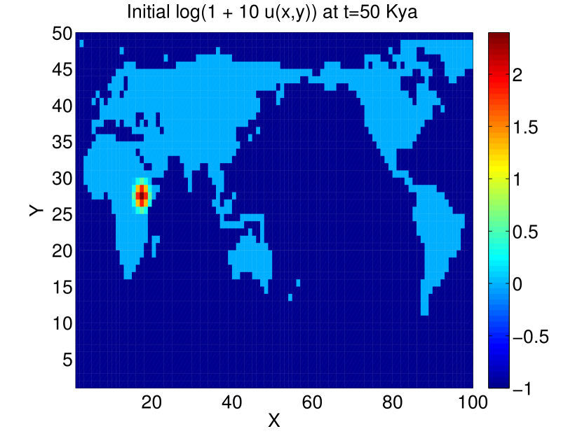
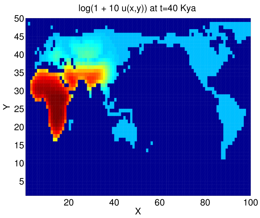
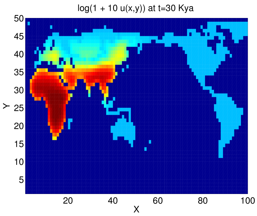
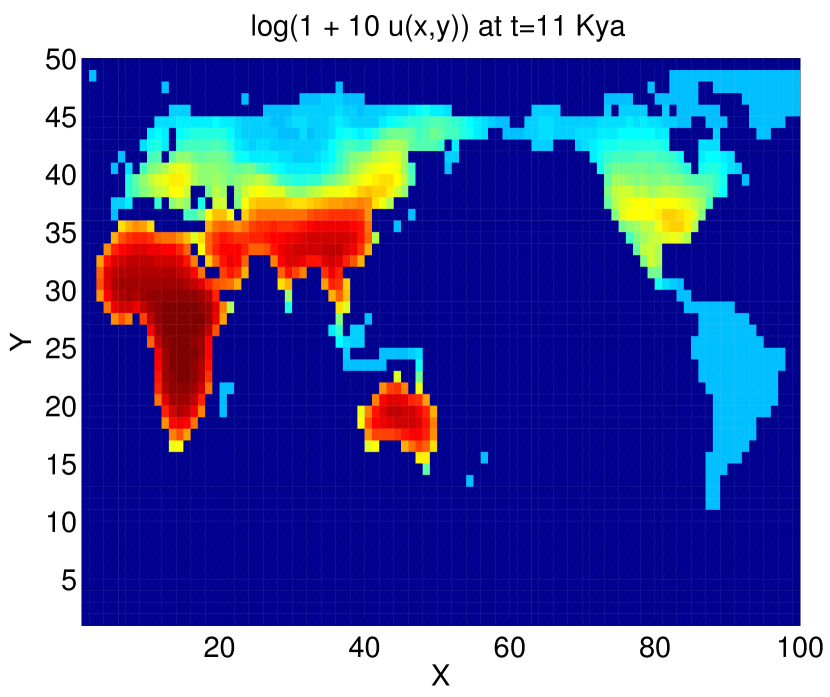
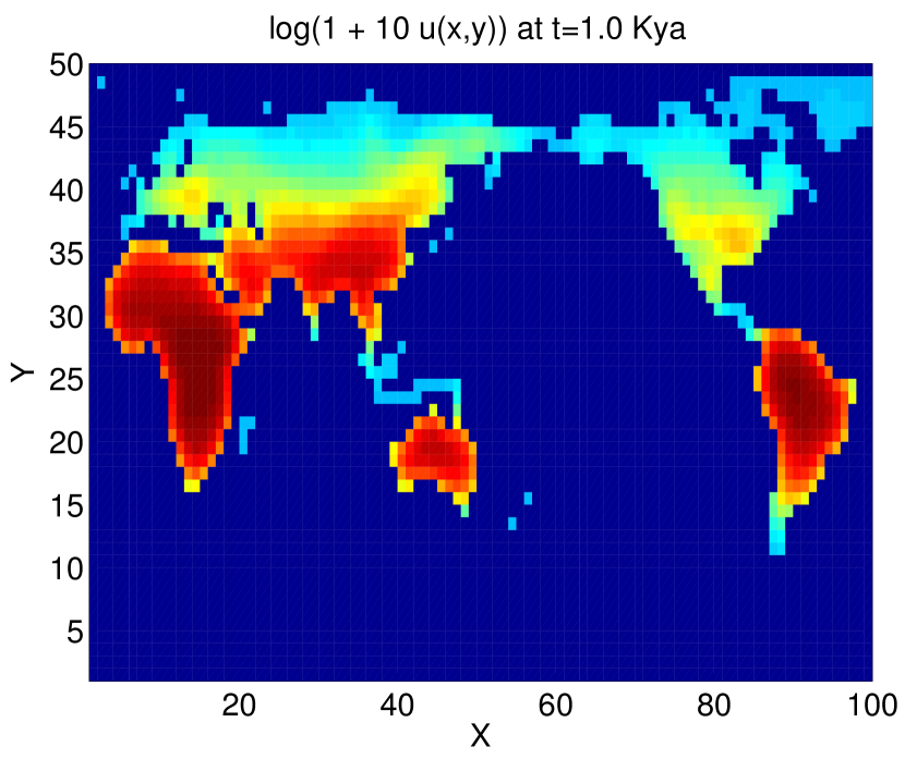
We set up the initial population density at $t=50$ kya as shown in the top left panel of Figure 9. The integration units are scaled following Tab. 1 such that $\lambda=1.67\cdot 10^{-3}$ ky^-1 and $c=208$ km²/ky (consistent with those used in (Young and Bettinger, 1995)). The solver is then run using time frame $\mathcal{K}$ maps described above, down to 1 kya. The remaining plots (Figures 10,11) display the resulting population dispersal simulation on unsmoothed $\mathcal{K}$ maps, regularized by (13). Using population parameters consistent with the literature, the gross features of the late (50-60 kya) out-of-Africa dispersal of Homo sapiens are reproduced (Forster, 2004), e.g. the colonization of Western Europe by $\sim 40$ kya and that of South America before 14 kya. Using the solver with the same initial conditions but on a smooth NPP map, like the one shown in right panel of Figure 7, without the regularizer (13), yields the same wavefront propagation speed.

6 Conclusions

In this paper, we presented a novel semi-implicit Godunov scheme for the Fisher/KPP equation with a constant carrying capacity $\mathcal{K}$, described in Section 3. In one dimension, the expected traveling wave (Fisher, 1937; Kolmogorov et al., 1937) develops as shown in Figure 1. In other tests, not shown here, we saw that almost any concentrated inital condition will develop similar waves: for example, two nearby peaks. Our scheme is on a rectangular grid, so in 2-D we need to ensure that in cylindrically symmetric situations we can control the errors due to the $x-y$ asymmetry. The error plots, Figure 4, show that we can reduce the asymmetries somewhat by an alternating direction scheme. In any case, these errors are very small even for a relatively high CFL number. As in the one-dimensional situation, a traveling wave also develops as expected (Kolmogorov et al., 1937): Figure 2 and Figure 3 show this development and compare the results to the 2-D symmetric version of the Matlab function pdepe. Because the $\mathbf{x}$ discretization has truncation errors proportional to $(\Delta x)^{3}$, after $O(\frac{1}{h})$ time steps we should not be surprised to see the errors shown in Figure 3 turn up for very small $h$ and behave roughly as $O(\frac{1}{h}(\Delta x)^{3})$.

In Secs. 4.1 we extended our procedure to handle an $\mathbf{x}$-dependent $\mathcal{K}$, specifically eq. (11). In order to regularize our solver against bad behavior when dealing with $\mathcal{K}$ maps inferred from real-world data, in Section 4.2 we studied both regularization and the expected constant velocity of the traveling wave. Except for small transition regions entering or leaving a region of low carrying capacity, the velocity ($\sqrt{2}$ in our scaling) is indeed constant. In Section 4.4, we went further to develop a scheme for the situation with both $\mathbf{x}$ and $t$ dependent carrying capacity $\mathcal{K}$ via eq.(16).

Finally, this scheme has been applied to a prototypical case in population dynamics: the out-of-Africa dispersal of Homo sapiens. On the Mercator projected world map, by using vegetation net primal productivity as a proxy for carrying capacity, Figure 9 shows that by the regularization of $\mathcal{K}$ in space via eq. (13) but interpolating in time yields stable and reasonable results. In fact, the results showing ancestor arrival in NE India at roughly 40 kya, then crossing the Bering Strait before 10 kya, and multiple routes into South Asia (Reyes-Centento et al., 2014) are very encouraging. Honesty requires that we admit our size (408km)² pixels do not resolve the two crossing points at Bab al Mendab and Sinai adequately. Additionally, a switch (see: Section 4.5) which would allow passage at the Bering Strait seems unnecessary due to the interesting coincidence that the hominin wave front reaches this passage at the beginning of the last ice age. If it were blocked previously, this would have had no effect.

The core computations performed by our solver are independent tridiagonal solutions, which can be easily parallelized to deal with larger grids. In order to further improve numerical performance, in the Appendix A, we discussed a compressed storage scheme to integrate the Fisher/KPP equation on a projected world map (or any other irregularly-shaped domain). The alternating direction scheme discussed in Section 3.2 also works with this compressed storage. In the case of world dispersal discussed in Section 5, since about 71% of the earth’s surface is water, this compressed storage reduces computational work by the same amount.

Provenance

For this paper, the simulations were run on either a Mac Mini, 2.4 GHz Intel Core Duo (Mac OS 10.6.8), or a MacBook laptop with the same processor specifications but running OS 10.8.4. On the Mini, MatLab (7.10.0.499) R2010a was used, respectively (8.1.0.604) R2013a on the MacBook laptop.

Appendix A Map segmentation appendix

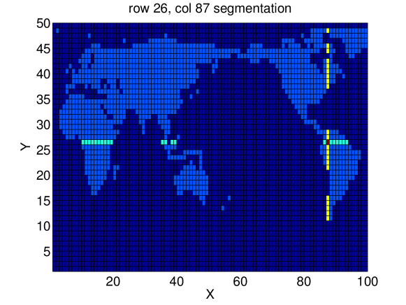
In order to use our solver on a geographical map, it suffices to use a map outline, i.e., a rectangular grid with 1’s in habitable regions, and 0’s in the water, as in Figure 12. Since each Godunov direction step only involves a row, or a column, independently, we can set up the following indexing scheme. Each row $i=1\dots 50$ in Figure 12 will have nysegs(i) of habitable segments, whose starting and ending positions are ystart_seg(k) and yend_seg(k), respectively, where $k=1\dots$nysegs(i). Likewise, for $j=1\dots 100$ columns each with nxsegs(j) also with start and end positions. Roughly 24% of the world map is land, i.e. habitable. As an example, Figure 12 shows row 26 has 4 segments of varying size. Likewise, column 87 has 5 segments. A sample MatLab code in Appendix A illustrates the scheme for 1/2 step of $x$-direction updates, followed by a full step of $y$-direction updates, then again 1/2 step of $x$-direction segment updates. The alternating direction method, described in Section 3.2, just interchanges $x\leftrightarrow y$ on alternate time steps.

For the reader’s convenience, we include here a sample Matlab code of our Godunov-Strang-Yoshida scheme.

% NY X direction updates for half-step1
      locx = 0;
      for j=1:NY
          nsegs = nxsegs(j);
          for k=1:nsegs
              istart=xstart_seg(locx+k); iend=xend_seg(locx+k);
              ninseg=iend-istart+1;
              u0(1) = 0; u0(ninseg+2) = 0;  % boundary values
              u0(2:ninseg+1) = u(istart:iend,j);
% eq. (15a) solution:
              ut = godunovstep1(ninseg+2,h,kcfl,u0,sc1,sc2);
              u(istart:iend,j) = ut(2:ninseg+1);
          end
          locx = locx + nsegs;
      end
% NX Y direction updates step2
      locy = 0;
      for i=1:NX
          nsegs = nysegs(i);
          for k=1:nsegs
              jstart=ystart_seg(locy+k); jend=yend_seg(locy+k);
              ninseg=jend-jstart+1;
              u1(1) = 0; u1(ninseg+2) = 0; % boundary values
              u1(2:ninseg+1) = u(i,jstart:jend)’;
              cap(1) = 1; cap(ninseg+2) = 1;
              cap(2:ninseg+1) = kap(i,jstart:jend);
% eq. (15c) solution:
              ut = godunovstep2(ninseg+2,h,kcfl,u1,sc1,sc2,cap);
              u(i,jstart:jend) = ut(2:ninseg+1);
          end
          locy = locy + nsegs;
      end
% Repeat godunovstep1, as above for eq. (15d)
%     locx = 0;
%     for j=1:NY
%         ETC
%     end

Figure 1: Left: Godunov vs. pdepe at the end of one time step $t=h$. Right: Godunov vs. pedpe at time $t=30$. The time step $h=1/5$ and $\Delta x=1/5$.

Figure 2: Left: 2-D solution at $t=5$ obtained with Godunov scheme (9). Right: same, at $t=20$. The time step was $h=1/10$, $\Delta x=2/5$ and $N_{X}=N_{Y}=201$.

Figure 3: Left: 2-D Wave front at $t=20$ compared to pdepe. Right: Rough RMS error as a function of step size, $h$, at $t=20$. Errors $\epsilon_{RMS}$ and $\epsilon_{MAX}\approx 3.5\epsilon_{RMS}$ have approximately $O(h^{2})$ behavior for $h\geq 1/10$, but increase if $h$ is too small: overall estimate is $O(h^{2})+O(\Delta x^{2})+O(\frac{1}{h}\Delta x^{3})$.

Figure 4: Left: $|u(x,y)-u(r)|$ error profile of the Godunov scheme compared to the pdepe solution at $t=20$ symmetrizing $x\leftrightarrow y$ on alternate time steps: $\epsilon_{RMS}=7.3\cdot 10^{-3}$, $\epsilon_{MAX}=2.9\cdot 10^{-2}$. Right: the same, but with fixed $x$ and $y$: $\epsilon_{RMS}=7.4\cdot 10^{-3}$, $\epsilon_{MAX}=3.0\cdot 10^{-2}$. Step size is $h=1/10$, $N_{x}=N_{y}=401$.

Figure 5: Left: desert test density at $t=37.5$: $N_{x}=201$, $N_{y}=101$, and $h=1/8$. For $x\leq-16$ and $x\geq 16$, $\mathcal{K}=1$, while $\mathcal{K}=f_{r}=0.01$ in the $|x|<16$ desert. The image shows $u(x,y)$ shaded from 0 (black) to 1 (white). The wave can be seen crossing into the upper $\mathcal{K}=1$ region, while the population in the lower $\mathcal{K}=1$ region has already saturated. Right: half-height $x_{1/2}(t)$ of the wave front vs. time, compared with pdepe. Velocity $V$ has a transient increase, then decrease, as the wave enters/exits the desert. Initial condition: a strip with $\langle(x-x_{I})^{2}\rangle^{1/2}=3$ initial population starting at $x_{I}=-30$.

Figure 6: Regularizers for eq. (14).

Figure 7: Left: Siberia rough 50kya NPP distribution. Note the $\mathcal{K}=0$ hole at pixel $\mbox{north}=14$, $\mbox{east}=38$. Right: same sub-map but smoothed by the low pass filter (15). Scales are $\log{(1+10\mathcal{K})}$ with the original $0.3\leq\mathcal{K}\leq 3\times 10^{4}$ biomass units (gm/$\mbox{m}^{2}$) (Grieser et al., 2006). Both plots use the same colorbar.

Figure 8: Interpolation between $\mathcal{K}$ maps at different times: sigmoids (18) for $\nu=1/2$ and $\nu=1$, straight line, and Eriksson’s $f(f(f(t)))$ model (Eriksson et al., 2012).

Figure 9: Color-coded $\log{(1+10u)}$ plot for out-of-Africa dispersal. Dark blue shows water, with $\mathcal{K}=0$. Growth rate is $\lambda=1.67\cdot 10^{-3}\,\mathrm{ky}^{-1}$, and diffusion coefficient $c=208\,\mathrm{km}^{2}\mathrm{/ky}$ (Young and Bettinger, 1995). Left: initial distribution at $t=50$ kya. This color scale is used in all subsequent dispersal plots below. Right: differences between the regularization (13) of $u$ vs. smoothing of $\mathcal{K}(\mathbf{x},t)$ (15) at $t=1$ kya.

Figure 10: Out of Africa simulations by regularization (13). Left: population at $t=40$ kya. Right: population at $t=30$ kya. Color scale is from Fig. 9 (left).

Figure 11: Out of Africa simulations with regularization (13). Left: population at $t=11$ kya. Right: population at $t=1$ kya. Color scale is from Fig. 9 (left).

Figure 12: Map with habitable regions set to 1 (light blue) and water regions set to 0 (dark blue) on a $N_{x}=100$, $N_{y}=50$ grid. The figure shows the segmentation for row 26 and column 87, with 4 and 5 segments, shown in cyan and yellow respectively.

References

- Bigelow et al. (2003) Nancy H Bigelow, Linda B Brubaker, Mary E Edwards, Sandy P Harrison, I Colin Prentice, Patricia M Anderson, Andrei A Andreev, Patrick J Bartlein, Torben R Christensen, Wolfgang Cramer, et al. Climate change and arctic ecosystems: 1. vegetation changes north of 55 n between the last glacial maximum, mid-holocene, and present. J. of Geophysical Research, 108(D19):8170, 2003.
- Bouckaert et al. (2012) Remco Bouckaert, Philippe Lemey, Michael Dunn, Simon J Greenhill, Alexander V Alekseyenko, Alexei J Drummond, Russell D Gray, Marc A Suchard, and Quentin D Atkinson. Mapping the origins and expansion of the indo-european language family. Science, 337(6097):957–960, 2012.
- (3) bridgeproj. URL: http://www.bridge.bris.ac.uk, 2003.
- Callegari et al. (2013) Simone Callegari, John David Weissmann, Natalie Tkachenko, Wesley P Petersen, George Lake, Marcia Ponce de León, and Christoph PE Zollikofer. An agent-based model of human dispersals at a global scale. Advances in Complex Systems, 16(4), 2013.
- Eriksson et al. (2012) Anders Eriksson, Lia Betti, Andrew D Friend, Stephen J Lycett, Joy S Singarayer, Noreen von Cramon-Taubadel, Paul J Valdes, Francois Balloux, and Andrea Manica. Late pleistocene climate change and the global expansion of anatomically modern humans. Proceedings of the National Academy of Sciences, 109(40):16089–16094, 2012.
- Fisher (1937) Ronald Aylmer Fisher. The wave of advance of advantageous genes. Annals of Eugenics, 7(4):355–369, 1937.
- Forster (2004) Peter Forster. Ice ages and the mitochondrial dna chronology of human dispersals: a review. Philosophical Transactions of the Royal Society of London. Series B: Biological Sciences, 359(1442):255–264, 2004.
- Godunov and Ryabenkii (1987) Sergei Konstantinovich Godunov and Victor Solomonovich Ryabenkii. Difference schemes: an introduction to the underlying theory. Elsevier, New York, 1987.
- Grieser et al. (2006) Jürgen Grieser, René Gommes, Stephen Cofield, and Michele Bernardi. World maps of climatological net primary production of biomass, NPP, 2006.
- Harrison et al. (2001) SP Harrison, G Yu, H Takahara, and IC Prentice. Palaeovegetation (communications arising): diversity of temperate plants in east asia. Nature, 413(6852):129–130, 2001.
- Henn et al. (2012) Brenna M Henn, LL Cavalli-Sforza, and Marcus W Feldman. The great human expansion. Proceedings of the National Academy of Sciences, 109(44):17758–17764, 2012.
- Higham and Higham (2005) Desmond J Higham and Nicholas J Higham. MATLAB guide. SIAM, Philadelphia, PA, 2005.
- Kolmogorov et al. (1937) AN Kolmogorov, IG Petrovsky, and NS Piskunov. Etude de l’équation de la diffusion avec croissance de la quantité de matiere et son applicationa un probleme biologique. Moscow Univ. Bull. Math, 1:1–25, 1937.
- LeVeque (2007) Randall J LeVeque. Finite difference methods for ordinary and partial differential equations: steady-state and time-dependent problems. SIAM, Philadelphia, PA, 2007.
- Lieth et al. (1975) Helmut H Lieth, Robert RH Whittaker, et al. Primary productivity of the biosphere. Springer-Verlag, New York, 1975.
- Manica et al. (2007) Andrea Manica, William Amos, François Balloux, and Tsunehiko Hanihara. The effect of ancient population bottlenecks on human phenotypic variation. Nature, 448(7151):346–348, 2007.
- Murray (2002) James Dickson Murray. Mathematical Biology. Springer-Verlag, New York, 2002.
- Nikitas and Nikita (2005) P Nikitas and E Nikita. A study of hominin dispersal out-of-Africa using computer simulations. J. of human evolution, 49(5):602–617, 2005.
- Pickett et al. (2004) Elizabeth J Pickett, Sandy P Harrison, Geoff Hope, Kate Harle, John R Dodson, A Peter Kershaw, I Colin Prentice, John Backhouse, Eric A Colhoun, Donna D’Costa, et al. Pollen-based reconstructions of biome distributions for australia, southeast asia and the pacific (seapac region) at 0, 6000 and 18,000 14c yr bp. J. of Biogeography, 31(9):1381–1444, 2004.
- Pinhasi et al. (2005) Ron Pinhasi, Joaquim Fort, and Albert J Ammerman. Tracing the origin and spread of agriculture in europe. PLoS Biology, 3(12):e410, 2005.
- Prentice and Jolly (2000) I Colin Prentice and Dominique Jolly. Mid-holocene and glacial-maximum vegetation geography of the northern continents and africa. J. of Biogeography, 27(3):507–519, 2000.
- Reichl (2004) Linda E. Reichl. A modern course in statistical physics. Wiley-VHC Verlag Gmbh, KGaH, Weinheim, 2004.
- Relethford (2004) John Relethford. Global patterns of isolation by distance based on genetic and morphological data. Human Biology, 76(4):499–513, 2004.
- Reyes-Centento et al. (2014) Hugo Reyes-Centento, Silvia Ghirotto, Florent Detroit, Dominique Grimaud-Herve, and Guido Barbujani. Genomic and cranial phenotype data support multiple modern human dispersals from africa and a southern route into asia. Proceedings of the National Academy of Sciences, April 21:doi:10.1073/pnas.1323666111, 2014.
- Ritchmyer and Morton (1967) Robert D Ritchmyer and KW Morton. Difference methods for initial-value problems, volume 1. Interscience Tracts in Pure and Applied Mathematics, New York: Interscience, 1967, 2nd ed., 1967.
- Siddall et al. (2003) Mark Siddall, Eelco J Rohling, A Almogi-Labin, Ch Hemleben, D Meischner, Ina Schmelzer, and DA Smeed. Sea-level fluctuations during the last glacial cycle. Nature, 423(6942):853–858, 2003.
- Skellam (1951) John Gordon Skellam. Random dispersal in theoretical populations. Biometrika, 38(1/2):196–218, 1951.
- Strang (1968) Gilbert Strang. On the construction and comparison of difference schemes. SIAM J. on Numerical Analysis, 5(3):506–517, 1968.
- Strang and Aarikka (1986) Gilbert Strang and Kaija Aarikka. Introduction to applied mathematics, volume 16. Wellesley-Cambridge Press Wellesley, MA, 1986.
- Yoshida (1990) Haruo Yoshida. Construction of higher order symplectic integrators. Physics Letters A, 150(5):262–268, 1990.
- Young and Bettinger (1995) David A Young and Robert L Bettinger. Simulating the global human expansion in the late pleistocene. J. of Archaeological Science, 22(1):89–92, 1995.