Polynomial-Chaos-based Kriging
Abstract
Computer simulation has become the standard tool in many engineering fields for designing and optimizing systems, as well as for assessing their reliability. Optimization and uncertainty quantification problems typically require a large number of runs of the computational model at hand, which may not be feasible with high-fidelity models directly. Thus surrogate models (a.k.a meta-models) have been increasingly investigated in the last decade. Polynomial Chaos Expansions (PCE) and Kriging are two popular non-intrusive meta-modelling techniques. PCE surrogates the computational model with a series of orthonormal polynomials in the input variables where polynomials are chosen in coherency with the probability distributions of those input variables. A least-square minimization technique may be used to determine the coefficients of the PCE. On the other hand, Kriging assumes that the computer model behaves as a realization of a Gaussian random process whose parameters are estimated from the available computer runs, i.e. input vectors and response values. These two techniques have been developed more or less in parallel so far with little interaction between the researchers in the two fields. In this paper, PC-Kriging is derived as a new non-intrusive meta-modeling approach combining PCE and Kriging. A sparse set of orthonormal polynomials (PCE) approximates the global behavior of the computational model whereas Kriging manages the local variability of the model output. An adaptive algorithm similar to the least angle regression algorithm determines the optimal sparse set of polynomials. PC-Kriging is validated on various benchmark analytical functions which are easy to sample for reference results. From the numerical investigations it is concluded that PC-Kriging performs better than or at least as good as the two distinct meta-modeling techniques. A larger gain in accuracy is obtained when the experimental design has a limited size, which is an asset when dealing with demanding computational models.
Keywords: Emulator – Gaussian process modeling – Kriging, meta-modelling – Polynomial Chaos Expansions – PC-Kriging – Sobol’ function
1 Introduction
Modern engineering makes a large use of computer simulation in order to design systems of ever increasing complexity and assess their performance. As an example, let us consider a structural engineer planning a new structure. An essential part of his work is to predict the behavior of the not-yet-built structure based on some assumptions and available information about e.g. acceptable dimensions, loads to be applied to the structure and material properties. These ingredients are basically the input parameters of computational models that predict the performance of the system under various conditions. The models help the engineer analyze/understand the behavior of the structure and eventually optimize the design in order to comply with safety and serviceability constraints.
Similar conditions can also be found in many other scientific and engineering disciplines. The common point is the simulation of the behavior of a physical process or system by dedicated algorithms which provide a numerical solution to the governing equations. These simulation algorithms aim at reproducing the physical process with the highest possible fidelity. As an example, finite element models have become a standard tool in modern civil and mechanical engineering. Due to high fidelity, such models typically exploit the available computer power, meaning that a single run of the model may take hours to days of computing, even when using a large number of CPUs.
An additional layer of complexity comes from the fact that most input parameters of such computational models are not perfectly known in practice. Some parameters (e.g. material properties, applied loads, etc.) may exhibit natural variability so that the exact value to be used for simulating the behavior of a particular system is not known in advance (this is referred to as aleatory uncertainty). Some others may have a unique value which is however not directly measurable and prone to lack of knowledge (epistemic uncertainty). In a probabilistic setup these parameters are modelled by random variables with prescribed joint probability density function, or more generally, by random fields. The goal of uncertainty propagation is to assess the effect of the input uncertainty onto the model output, and consequently onto the performance of the system under consideration (De Rocquigny et al., 2008; Sudret, 2007).
Propagating uncertainties usually requires a large number of repeated calls to the model for different values of the input parameters, for instance through a Monte Carlo simulation procedure. Such an approach usually require thousands to millions of runs which is not affordable even with modern high performance computing architectures. To circumvent this problem, surrogate models may be used, which replace the original computational model by an easy-to-evaluate function (Storlie et al., 2009; Hastie et al., 2001; Forrester et al., 2008). These surrogate models, also known as response surfaces or meta-models, are capable of quickly predicting responses to new input realizations. This allows for conducting analyses which require a large number of model evaluations, such as structural reliability and optimization, in a reasonable time.
Among the various options for constructing meta-models, this paper focuses on non-intrusive approaches, meaning that the computational model is considered as a “black-box model”: once an input vector (i.e. a realization of the random input in the process of uncertainty propagation) is selected, the model is run and provides an output vector of quantities of interest. No additional knowledge on the inner structure of the computer code is assumed. Popular types of meta-models that may be built from a limited set of runs of the original model (called the experimental design of computations) include Polynomial Chaos Expansions (PCE) Ghanem and Spanos (2003), Gaussian process modeling (also called Kriging) Sacks et al. (1989); Rasmussen and Williams (2006); Santner et al. (2003); Stein (1999), and support vector machines Gunn (1998); Smola and Schölkopf (2006); Vazquez and Walter (2003); Clarke et al. (2003), which have been extensively investigated in the last decade. Polynomial chaos expansions and Kriging are specifically of interest in this paper.
Polynomial chaos expansions (PCE), also know as spectral expansions, approximate the computational model by a series of multivariate polynomials which are orthogonal with respect to the distributions of the input random variables. Traditionally, spectral expansions have been used to solve partial differential equations in an intrusive manner Ghanem and Spanos (2003). In this setup truncated expansions are inserted into the governing equations and the expansion coefficients are obtained using a Galerkin scheme. This pioneering approach called spectral stochastic finite element method (SSFEM), was later developed by Xiu and Karniadakis (2002); Sudret et al. (2004); Wan and Karniadakis (2005, 2006); Berveiller et al. (2006a), among others. These intrusive methods require specific, problem-dependent algorithmic developments though. Because it is not always possible and/or feasible to treat a computational model intrusively, especially when legacy codes are at hand in an industrial context, non-intrusive polynomial chaos expansions were developed. So-called projections methods were developed by Ghiocel and Ghanem (2002); Le Maître et al. (2002); Keese and Matthies (2005); Xiu and Hesthaven (2005), see a review in Xiu (2009). Least-square minimization techniques have been introduced by Choi et al. (2004); Berveiller et al. (2006b); Sudret (2008). Further developments which combine spectral expansions and compressive sensing ideas have lead to so-called sparse polynomial chaos expansions Blatman and Sudret (2008, 2010a, 2010b); Doostan and Owhadi (2011); Blatman and Sudret (2011); Doostan et al. (2013); Jakeman et al. (2014). This is the approach followed in this paper. Further recent applications of PCE to structural reliability analysis and design optimization can be found in Eldred (2009); Eldred et al. (2008); Sarangi et al. (2014).
The second meta-modeling technique of interest in this paper is Kriging, which originates from interpolating geographical data in mining Krige (1951) and is today also known as Gaussian process modeling Rasmussen and Williams (2006); Santner et al. (2003). The Kriging meta-model is interpreted as the realization of a Gaussian process. Practical applications can be found in many fields, such as structural reliability analysis Kaymaz (2005); Bect et al. (2012); Echard et al. (2011); Bichon et al. (2008); Dubourg et al. (2013); Dubourg and Sudret (2014) and design optimization Jones et al. (1998); Dubourg et al. (2011); Dubourg (2011). The implementation of the Kriging meta-modeling technique can be found in e.g. the Matlab toolbox DACE Lophaven et al. (2002) and the more recent R toolbox DiceKriging Roustant et al. (2012, 2013).
So far the two distinct meta-modeling approaches have been applied in various fields rather independently. To our knowledge, there has not been any attempt to combine PCE and Kriging in a systematic way yet. To bridge the gap between the two communities, this paper aims at combining the two distinct approaches into a new and more powerful meta-modeling technique called Polynomial-Chaos-Kriging (PC-Kriging). As seen in the sequel the combination of the characteristics and the advantages of both approaches leads to a more accurate and flexible algorithm which will be detailed in this paper.
The paper is organized as follows. PCE and Kriging are first summarized in Section 2 and Section 3 respectively. Section 4 introduces the new meta-modeling approach PC-Kriging as the combination of the two distinct approaches. The accuracy of the new and traditional meta-modeling approaches is compared in Section 5 on a set of benchmark analytical functions.
2 Polynomial Chaos Expansions
2.1 Problem definition
Consider the probability space , where denotes the event space equipped with -algebra and the probability measure . Random variables are denoted by capital letters and their realizations denoted by the corresponding lower case letters, e.g. . Random vectors (e.g. ) and their realizations (e.g. ) are denoted by bold faced capital and lower case letters, respectively.
In this context, consider a system whose behavior is represented by a computational model which maps the -dimensional input parameter space to the -dimensional output space, i.e. where . As the input vector is assumed to be affected by uncertainty, a probabilistic framework is introduced. Due to uncertainties in the input vector, it is represented by a random vector with given joint probability density function (PDF) . For the sake of simplicity the components are assumed independent throughout the paper, so that the joint PDF may be written as the product of the marginal PDFs denoted by , . Note that the case of dependent input variables can easily be addressed by using an isoprobabilistic transform first, such as the Nataf or Rosenblatt transform Blatman and Sudret (2010a). The output of the model is a random variable obtained by propagating the input uncertainty in through the computational model :
| (1) |
In this paper we consider that the computational model is a deterministic mapping from the input to the output space, i.e. repeated evaluations with the same input value lead to the same output value .
Provided that the output random variable is a second-order variable (i.e. ), it can be cast as the following polynomial chaos expansion (PCE) Ghanem and Spanos (2003); Soize and Ghanem (2004):
| (2) |
where are coefficients of the multivariate orthonormal polynomials in coherency with the distribution of the input random vector , is the multi-index and is the number of input variables (dimensions). Since the components of are independent, the joint probability density function is the product of the margins . Then a functional inner product for each marginal PDF is defined by
| (3) |
for any two functions such that the integral exists. For each variable an orthonormal polynomial basis can be constructed which satisfies Xiu and Karniadakis (2002):
| (4) |
where are two candidate univariate polynomials in the -th variable, is the support of the random variable and is the Kronecker delta which is equal to 1 for and equal to otherwise. Xiu and Karniadakis (2002) summarize various orthonormal bases for some classical PDFs, some of which are summarized in Tab. 1.
| Distribution | Orthogonal polynomials | Orthonormal basis | |
|---|---|---|---|
| Uniform | Legendre | ||
| Gaussian | Hermite | ||
| Gamma | Laguerre | ||
| Beta | Jacobi | ||
The multivariate polynomials in Eq. (2) are then composed of univariate polynomials by tensor product, i.e. by multiplying the various polynomials in each input variable:
| (5) |
where is the polynomial of degree in the -th variable.
The main idea of polynomial chaos expansion (PCE) is then to surrogate the computational model by an infinite series of polynomials as shown in Eq. (2). In practice, it is not feasible to handle infinite series, thus the need of a truncation scheme. Such a truncation scheme corresponds to a set of multi-indexes such that the system response is accurately approximated with respect to some error measure Blatman and Sudret (2010a, 2011):
| (6) |
There are several ways to select a priori a truncation set . A simple and commonly applied scheme consists in upper-bounding the total degree of polynomials to a maximal value . The total degree of polynomials is defined by
| (7) |
In this case the set of multi-indices is denoted by where is the maximal total polynomial degree. The cardinality of the set reads:
| (8) |
This cardinality grows polynomially with both and . Such a truncation scheme thus leads to non tractable problems if the response is highly nonlinear in its input parameters (need for a large ) and/or if the size of the input vector is large (say, ). This problem is referred to as the curse of dimensionality.
Blatman and Sudret (2010a); Blatman (2009) proposed a more restrictive truncation scheme called hyperbolic truncation set. The authors observed that many systems tend to have only low-degree interaction polynomials and thus it is not necessary to compute all interaction terms of higher polynomial degree. The hyperbolic index set is based on the following -norm:
| (9) |
where
| (10) |
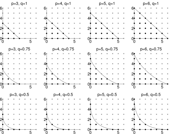
is a tuning parameter and is the maximal total degree of the polynomials. A decreasing leads to a smaller number of interactive polynomials, i.e. a smaller set of polynomials. When , only univariate polynomials are left in the set of polynomials which is called an additive model Sudret (2014). For the sake of illustration, the retained polynomial indices of a 2-dimensional input space () and varying and are illustrated in Figure 1. The indices denoted by are part of and the solid black line represents . Note that for , the hyperbolic index sets are equivalent to the total degree index set (see Eq. (7)).
2.2 Computation of the coefficients
After defining the set of candidate polynomials, the next step is to determine the expansion coefficients of each multivariate polynomial . In this paper we consider only non-intrusive methods which are based on repeatedly evaluating the model over a set of input realizations , the so-called experimental design. Different non-intrusive methods have been proposed in the last decade to calibrate PC meta-models, namely projection Ghiocel and Ghanem (2002); Le Maître et al. (2002); Keese and Matthies (2005), stochastic collocation Xiu and Hesthaven (2005); Xiu (2009) and least-square minimization methods Chkifa et al. (2013); Migliorati et al. (2014); Berveiller et al. (2006b); Blatman and Sudret (2010a, 2011). In this paper we adopt the least-square minimization method. The expansion coefficients are calculated by minimizing the expectation of the least-squares residual:
| (11) |
In practice the expectation in Eq. (11) is evaluated by an empirical sample-based estimator. Denoting by the set of outputs of the exact model for each point in the experimental design , the discretized least-squares error minimization problem derived from Eq. (11) reads
| (12) |
The optimal expansion coefficients may be computed by solving the linear system
| (13) |
where is the information matrix of size whose generic term reads:
| (14) |
Typically for smooth functions, a small number of polynomials is able to represent accurately the output of the computational model. Thus a further reduction of the set of predictors in high-dimensional space is possible. Various types of generalized regression algorithms have been proposed in the literature, namely the least absolute shrinkage operator (LASSO) Tibshirani (1996), the Least Angle Regression (LAR) Efron et al. (2004), low-rank approximations Doostan et al. (2013); Peng et al. (2014) and compressive sensing Sargsyan et al. (2014). In the applications of this paper, the LAR algorithm is used in combination with hyperbolic index sets.
Given a PCE meta-model, i.e. a set of polynomials and the corresponding parameters , the response of a new sample may be eventually predicted by Eq. (6):
| (15) |
2.3 Error estimation
As seen in Eq. (6), polynomial chaos expansions (PCE) are approximations of the exact computational model and thus the prediction at new input samples leads to some residual error. That is why error measures are developed to quantify the deviation between the exact output and the meta-model output . The generalization error (also called -error) is the expectation of the squared output residuals Vapnik (1995), i.e.
| (16) |
where corresponds to the truncated series (see Eq. (6)) and the expectation is defined with respect to the PDF of the input variables . If the computational model is inexpensive to evaluate, the generalization error can be estimated accurately using an auxiliary validation set , which is sampled from the input distribution . The estimate of the generalization error then reads:
| (17) |
However, this rarely happens in real applications since the very purpose of building a meta-model is to avoid evaluating on a large sample set . Note that in Section 5 though, the various meta-modeling techniques are compared on analytical benchmark functions, making it possible to use such an estimate of the generalization error.
When the use of a large validation set is not affordable, the empirical error based on the available experimental design may be defined:
| (18) |
Normalizing the empirical error by the variance of the output values leads to the relative empirical error which is defined as
| (19) |
where is the mean value of the output values . The empirical error which is based on the experimental design generally underestimates the generalization error. In particular if the number of polynomials is close to the number of samples in the experimental design, the empirical error tends to zero whereas the true (generalization) error does not. This phenomenon is called overfitting (in the extreme case where the predictors may interpolate the experimental design points and thus the empirical error vanishes). Hence the leave-one-out (LOO) error has been proposed as an estimate of the generalization error Stone (1974); Geisser (1975). The general formulation of the leave-one-out error is
| (20) |
where is a PCE model built from the sample set and are the response values of the exact computational model. The LOO error is a special case of the leave--out cross-validation error Allen (1971) which discards samples from the initial experimental design to build up a model and predict the error at the discarded samples.
In theory the computational cost of the LOO error is proportional to the number of samples since it would require the determination of PCE meta-models corresponding to each experimental design . In the special case of linearly parameterized regression, which is the case for PCE, it is possible to calculate the LOO error analytically without building separate models. The LOO error reads (see e.g. Saporta (2006); Blatman (2009) for the proof)
| (21) |
where is the diagonal term of the matrix and the information matrix is defined in Eq. (14). Note that the PCE used in Eq. (21) is built only once from the full experimental design .
3 Kriging
3.1 Problem definition
The second meta-modeling technique in this paper is Kriging, also known as Gaussian process modeling, which assumes that the response of a computational model is a realization of a Gaussian random process Santner et al. (2003), i.e.
| (22) |
where is the mean value of the Gaussian process, also called trend, with coefficients , is the Gaussian process variance and is a zero-mean, unit-variance stationary Gaussian process. The zero-mean Gaussian process is fully determined by the auto-correlation function between two input sample points due to stationarity, where are hyper-parameters to be computed.
Various correlation functions can be found in the literature Rasmussen and Williams (2006); Santner et al. (2003), some of which are the linear, exponential, Gaussian (also called squared exponential) and Matérn autocorrelation function. In this paper the Matérn autocorrelation function is mainly used as it is a generalization of the exponential and the Gaussian autocorrelation functions. The general Matérn kernel of degree is defined as Matérn (1986)
| (23) |
where and are two sample points in the input space , are the scale parameters (also called correlation lengths), is the shape parameter, is the Euler Gamma function and is the modified Bessel function of the second kind (also known as Bessel function of the third kind). In many publications the shape parameter is set to either or which simplifies Eq. (23) to Roustant et al. (2012):
| (24) |
| (25) |
Apart from the correlation part in Eq. (22) there is also a trend part . Three different flavors of Kriging are defined in the literature Rasmussen and Williams (2006); Santner et al. (2003); Stein (1999), namely simple, ordinary and universal Kriging according to the choice of the trend. Simple Kriging assumes that the trend has a known constant value, i.e. . In ordinary Kriging the trend has a constant but unknown value, i.e. , and is unknown. The most general and flexible formulation is universal Kriging which assumes that the trend is composed of a sum of pre-selected functions , i.e.
| (26) |
where is the trend coefficient of each function. Note that simple and ordinary Kriging are special cases of universal Kriging. As discussed later in this paper, one approach to set up a trend is to use a sparse set of polynomials, which defines a new variant of universal Kriging.
3.2 Calibration of the Kriging model
Given a value for the auto-correlation hyper-parameters , the calibration of the Kriging model parameters may be computed using an empirical best linear unbiased estimator (BLUE). The optimization yields an analytical expression as a function of :
| (27) |
| (28) |
where are model responses of the exact computational model on the experimental design , is the correlation matrix and is the information matrix.
In recent developments, the optimal correlation parameters may be determined by either a maximum-likelihood-estimate (denoted by ML) Marrel et al. (2008); Dubourg (2011) or by leave-one-out cross-validation (CV) Bachoc (2013b). The optimal parameters are determined through a minimization which reads:
| (29) |
| (30) |
The comparison of both approaches shows that ML is preferable to CV in well-specified cases, i.e. when the meta-model autocorrelation function family is identical to the autocorrelation function of the computational model. For practical problems, i.e. assuming a black-box model, the autocorrelation function family is not known with certainty. In this case CV shall lead to more robust results than ML, as discussed in Bachoc (2013b).
Determining the optimal correlation parameters in Eq. (29) and (30) is a complex multi-dimensional minimization problem. Optimization algorithms can be cast into two distinct categories: local and global optimization algorithms. Local methods are usually gradient based algorithms such as the quasi-Newton Broyden-Fletcher-Goldfarb-Shanno (BFGS) algorithm Goldfarb (1970); Fletcher (1970); Shanno (1970) and its modifications Byrd et al. (1999). Global methods are algorithms such as genetic algorithms Goldberg (1989) and differential evolution algorithms Storn and Price (1997); Deng et al. (2013). The best optimization algorithm is problem dependent and in many cases not known a-priori.
The optimal correlation parameters are then used for predicting the model response at new samples of the input space. By assumption, the prediction of a Kriging model of a new point is a Gaussian random variable with mean and variance :
| (31) |
| (32) |
where is the correlation between the new sample and the sample of the experimental design. The prediction mean is used as the surrogate to the original model , whereas the variance gives a local error indicator about the precision. It is important to note that the Kriging model interpolates the data, i.e.
Apart from this procedure to calibrate the meta-model and predict model responses, the Kriging meta-modeling technique has been developed further in recent years. The latest developments in Kriging are contributed in the aspects of optimal estimation of the hyper-parameters Bachoc (2013b); Bachoc et al. (2014); Bachoc (2013a), the use of adaptive kernels Duvenaud et al. (2011); Ginsbourger et al. (2013) and the use of additive auto-correlation kernels Durrande et al. (2012, 2013); Ginsbourger et al. (2013)
3.3 Error estimation
A local error measure for any sample is given by the prediction variance in Eq. (32). This information is useful to detect regions where the prediction accuracy is low. Adding new samples to the experimental design in the regions with high prediction variance may lead to an overall increase in the accuracy of the meta-model in that region. This characteristics is exploited when devising adaptive experimental designs in structural reliability analysis, see Echard et al. (2013); Bichon et al. (2008); Bichon et al. (2011); Dubourg et al. (2011).
A simple global error measure of the accuracy of the meta-model (such as Eq. (19) for PC expansions) is not available for Kriging due to its interpolating properties, which make the empirical error vanish (considering no nugget effect in its auto-correlation function). Thus one approach to a global error measure is the leave-one-out (LOO) error
| (33) |
where is the prediction mean of sample by a Kriging meta-model based on the experimental design and is the exact model response. Dubrule (1983) derived an analytical solution for the LOO error for universal Kriging without computing the meta-models explicitly in the same spirit as Eq. (21) for PC expansions. The prediction mean and variance are given by
| (34) |
| (35) |
where is a square matrix of size with and denoting the number of samples in the experimental design and the number of polynomials in the trend part, respectively:
| (36) |
where is the Kriging variance for the full experimental design estimated by Eq. (28). A generalized version of this algorithm called v-fold cross-correlation error can be found in Dubrule (1983).
3.4 PCE as a particular case of universal Kriging
PC expansions can be interpreted as Kriging models where the samples of the experimental design are uncorrelated, i.e. where the autocorrelation function consists of the Dirac function:
| (37) |
The correlation matrix is then the identity matrix of size , i.e. . This reduces Eq. (27) to Eq. (13) and Eq. (31) to Eq. (2).
Further it can be shown that the leave-one-out error in Eq. (33)-(35) reduces to Eq. (21) by the following derivations. Consider the symmetric partitioned matrix and the corresponding inverse , i.e. which are defined as:
where (resp. ) are square matrices with dimension (resp. ). Using block matrix inversion one can derive:
| (38) |
In the context of the leave-one-out error, taking in Eq. (36), , , :
| (39) |
Then, the leave-one-out error in Eq. (33) combined with Eq. (34) and the above inverse formulation of the matrix reads:
| (40) |
which is equivalent to the formulation of the leave-one-out error in Eq. (21) for the case of PCE and . Thus the leave-one-out error in PCE can be seen as a special case of the leave-one-out error in the Kriging framework.
4 PC-Kriging
4.1 Principle
The characteristic of Kriging is to interpolate local variations of the output of the computational model as a function of the neighboring experimental design points. In contrast, polynomial chaos expansions (PCE) are used for approximating the global behavior of using a set of orthogonal polynomials. By combining the two techniques we aim at capturing the global behavior of the computational model with the set of orthogonal polynomials in the trend of a universal Kriging model and the local variability with the Gaussian process. The new approach called Polynomial-Chaos-Kriging (PC-Kriging) combines these two distinct meta-modeling techniques and their characteristics.
Using now the standard notation for truncated polynomial chaos expansions (see Eq. (6)), we cast the PC-Kriging meta-model as follows Schöbi and Sudret (2014c):
| (41) |
where is a weighted sum of orthonormal polynomials describing the mean value of the Gaussian process and is the index set of the polynomials. is a zero-mean, unit-variance stationary Gaussian process defined by an autocorrelation function and is parametrized by a set of hyper-parameters .
Building a PC-Kriging meta-model consists of two parts: the determination of the optimal set of polynomials contained in the regression part (i.e. the truncation set ) and the calibration of the correlation hyper-parameters as well as the Kriging parameters . The set of polynomials is determined using the Least-Angle-Regression (LAR) algorithm as in Blatman and Sudret (2011) together with hyperbolic index sets to obtain sparse sets of polynomials. After the set of polynomials is fixed, the trend and correlation parameters are evaluated using the universal Kriging equations (Eq. (27)-(30)).
4.2 Algorithm
The two distinct frameworks for PCE and Kriging can be combined in various ways. In this paper two approaches will be explained in detail, i.e. the Sequential PC-Kriging (SPC-Kriging) and the Optimal PC-Kriging (OPC-Kriging). Both approaches are based on the same input information, namely the experimental design , the corresponding response values obtained from the computational model , the description of the stochastic input variables (joint PDF ) and the parametric expression of the an auto-correlation function . The two approaches are defined as follows:
-
•
Sequential PC-Kriging (SPC-Kriging): in this approach, the set of polynomials and the Kriging meta-model are determined sequentially. The assumption behind this procedure is that the optimal set of polynomials found by the LAR algorithm in the context of pure PCE can be used directly as an optimal trend for the universal Kriging. In a first step the optimal set of polynomials is determined using the PCE framework: is found by applying the LAR procedure as in Blatman and Sudret (2011). The set of multivariate orthonormal polynomials is then embedded into a universal Kriging model as the trend. The universal Kriging meta-model is calibrated using Eq. (27)-(30).
At the end of the algorithm the accuracy of the meta-model can be measured by the leave-one-out error given in Eq. (33) or, when using a validation set, by the sample-based generalization error in Eq. (17).
The SPC-Kriging algorithm is illustrated in Figure 2 in which the white boxes represent the required input information and the blue boxes represent the computational tasks. Given a calibrated SPC-Kriging model, the response of new input realizations (i.e. the prediction) is computed by Eq. (31) and Eq. (32).Figure 2: Flowchart for Sequential-PC-Kriging (SPC-Kriging) -
•
Optimal PC-Kriging (OPC-Kriging): in this approach, the PC-Kriging meta-model is obtained iteratively. The set of orthonormal multivariate polynomials is determined by LAR algorithm in the same way as in SPC-Kriging. Yet the LAR algorithm results in a list of ranked polynomials which are chosen depending on their correlation to the current residual at each iteration in decreasing order. OPC-Kriging consists of an iterative algorithm where each polynomial is added one-by-one to the trend part. In each iteration, the coefficients of the trend and the parameters of the auto-correlation function are calibrated. In the end, a number of different PC-Kriging models are available. The meta-models are then compared in terms of the LOO error (Eq. (33)). The optimal PC-Kriging meta-model is then chosen as the one with minimal leave-one-out error.
Figure 3 illustrates the OPC-Kriging algorithm in a flowchart. The notation means a universal Kriging meta-model where the trend is modeled by the first polynomials selected in according to the ranking obtained by LAR. Note that the red box represents the universal Kriging model which eventually minimizes the LOO error () and which is thus finally chosen. The final box marks the prediction of new model responses which is computed by Eq. (31) and Eq. (32).
As a summary PC-Kriging can be viewed as a universal Kriging meta-model with a non-standard trend part. Thus the error estimates from Kriging in Section 3.3 are valid here with no modification. In particular, the LOO error in Eq. (33) is computed to compare different PC-Kriging models and to compute the optimal meta-model in OPC-Kriging. The performance of both approaches and the comparison to the traditional PCE and Kriging approaches is now illustrated for a variety of benchmark analytical functions.
5 Analytical benchmark functions
5.1 Setup
Easy-to-evaluate functions are tested to verify and validate the new PC-Kriging approach by comparing the meta-model to the exact model response. In this paper, six analytical functions of different dimensionality are illustrated, namely four with uniformly distributed input variables (i.e. Ishigami, Sobol’, Rosenbrock and Morris functions) and two with Gaussian input variables (i.e. Rastrigin and O’Hagan function). References to the original use of the benchmark functions in the literature are given below.
The first four analytical functions use uniformly distributed random variables in the input space. The Ishigami function is a smooth function with three independent input parameters commonly used for benchmarking methods in global sensitivity analysis.
| (42) |
where . The Sobol’ function is also well-known sensitivity analysis because the Sobol’ indices are easy to derive analytically Sobol’ (1993):
| (43) |
where and as in Sudret (2008). Due to the absolute value operator in the enumerator the function behaves non-smoothly at the point . The Rosenbrock function is a polynomial function with a 2-dimensional input space Rosenbrock (1960):
| (44) |
where . The last function considered is the Morris function which is defined by Morris (1991)
| (45) |
where and for all except for where . The coefficients are defined as: ; ; . The remaining coefficients are set equal to and as in Blatman (2009).
Two other benchmark functions of independent Gaussian variables are also studied. The Rastrigin function has a two-dimensional input space and is defined by Rastrigin (1974)
| (46) |
where . The last function is the O’Hagan function which is defined by Oakley and O’Hagan (2004)
| (47) |
where . The vectors and matrix are defined in Oakley and O’Hagan (2004).
Note that the functions have uniform input random variables. Accordingly the PC trend in PC-Kriging is built up from multivariate Legendre polynomials. In contrast have Gaussian input random variables. Thus the PC trend is modeled by multivariate Hermite polynomials (see Tab. 1).
5.2 Analysis
At the beginning of each algorithm the experimental design is generated with the Latin-hypercube sampling technique McKay et al. (1979). Then the meta-modeling is processed applying the four previously discussed meta-modeling techniques, i.e. ordinary Kriging, PCE, SPC-Kriging and OPC-Kriging. Note that for the Kriging meta-models, the maximum likelihood formulation (Eq. (29)) in combination with the gradient based BFGS optimization algorithm is used in order to compute the optimal correlation parameters.
Their performance is compared by means of the relative generalization error which is defined as the ratio between the generalization error (Eq. (16)) and the output variance:
| (48) |
The error is estimated here using a large validation set of size , which results in
| (49) |
where is the mean value of the set of exact model responses over the validation set . For all Kriging-based approaches, the meta-model is the prediction mean . Note that the samples in follow the distribution of the input variables in order to obtain a reliable error estimate.
For each experimental setup, the analysis is replicated to account for the statistical uncertainties in the experimental design. 50 independent runs of the full analysis are carried out and the results are represented using boxplots. In a box plot the central mark represents the median value of the 50 runs, the edges are the 25th and 75th percentile denoted by and . The whiskers describe the boundary to the outliers. Outliers are defined as the values smaller than or larger than .
5.3 Results
5.3.1 Visualization of PC-Kriging’s behavior
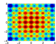
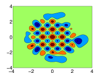
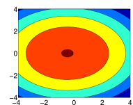
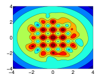
The different types of meta-models are illustrated in Fig. 4 which shows a 2-dimensional contour plot of the output of the Rastrigin function ( samples) (Fig. 4(A)) and its approximations by PCE, ordinary Kriging and PC-Kriging (Fig. 4(B)-4(D)). The Rastrigin function has a highly oscillatory behavior on the entire input space as seen in Fig. 4(A). This behavior is difficult to meta-model with a small number of samples because many local minima/maxima are missed out.
The analytical formulation of the Rastrigin function is a combination of a quadratic component and a high-frequency trigonometric component. The PCE model in Fig. 4(C) captures the global characteristic of the function, i.e. the quadratic component, whereas the ordinary Kriging model in Fig. 4(B) approximates the local characteristics, i.e. the high-frequency trigonometric component. Finally, the combination of PCE and Kriging leads to a better meta-model as shown in Fig. 4(D).
Note that the meta-models in Fig. 4 have a high accuracy around the origin of the coordinate system due to the definition of the input vector PDF as standard normal distributions ().
5.3.2 Small experimental design
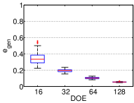
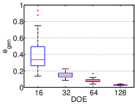
The four meta-modeling techniques are compared for the six analytical functions using experimental designs of increasing size. The number of samples is chosen so that it yields a large range of relative generalization errors on the second axis. The results are illustrated in Fig. 5-10. In each figure (A) shows the ordinary Kriging model and (B) shows the PCE model. The new approaches SPC-Kriging and OPC-Kriging are shown in (C) and (D) respectively.
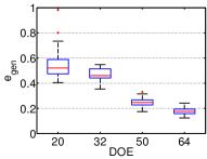
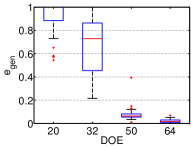
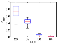
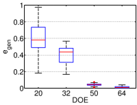
Figure 5 shows the relative generalization error for the various meta-modeling techniques for the Ishigami function. For a small sample size of samples, ordinary Kriging performs best with respect to the median value of the box plots. SPC-Kriging and OPC-Kriging perform worse due to the effect of overfitting (see also Section 2.3). The number of parameters to be estimated in the case of PC-Kriging is larger than in the case of ordinary Kriging due to the number of polynomials in the trend of the Kriging model. Thus, OPC-Kriging (and also SPC-Kriging) are more prone to overfitting than ordinary Kriging for small experimental designs. When the number of samples is increased, however, the two PC-Kriging approaches perform better than the traditional approaches because their median value and their variation of the error are lower. For the large sample sizes (), PC-Kriging performs similarly to PCE, though slightly better. OPC-Kriging is slightly more accurate than SPC-Kriging over the whole range of sample sizes.
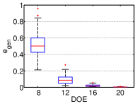
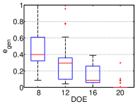
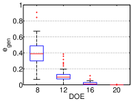
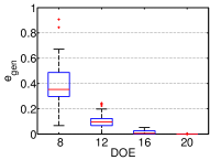
Figure 6 presents the results of the Rosenbrock function, which is a purely polynomial function and can be modeled accordingly with a small number of polynomials based on a small number of points in the experimental design (e.g. in the case of PCE). This is the reason why the number of points lies within . Highly accurate surrogate models are obtained with only 20 samples. For small sample sizes OPC-Kriging performs best among the four techniques in terms of the relative generalization error.
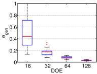
The Sobol’ function is more complex than the two previous functions because of the dimensionality () and the non-smooth behavior at . Thus more samples are needed to obtain a similar range of relative generalization errors compared to the previous functions, as seen in Fig. 7. Behaviors for the larger sample sizes () are very similar among the meta-modeling approaches, although PC-Kriging performs slightly better than the traditional PCE and ordinary Kriging approaches. For very small sample sizes (), OPC-Kriging performs significantly better than the others.
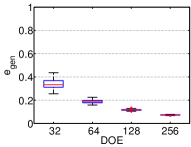
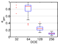
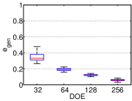
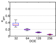
Figure 8 shows the results for the Morris function. A large experimental design is required to properly surrogate the computational model because of the high dimensionality of the input vector and the amount of interactive terms of different input variables in the analytical formulation (see Eq. (45)). The relative generalization error of the two PC-Kriging approaches resembles more the one of ordinary Kriging than the one of PCE in this case. PCE is not capable of modeling this analytical function with a small number of samples.
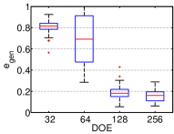
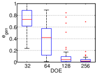
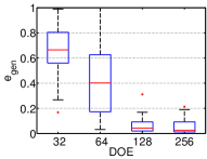
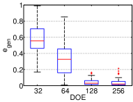
The results associated with the Rastrigin function are shown in Fig. 9. Despite the low dimensionality of the input (), many samples are needed to obtain small error estimates. This is due to the fact that the function output is highly oscillatory over the entire input space as previously illustrated in Fig. 4. In comparison to Section 5.3.1, which describes the qualitative performance of PC-Kriging on the Rastrigin function, the quantitative benefit of combining PCE and Kriging becomes visible in Fig. 9: PC-Kriging performs better than the traditional approaches. Ordinary Kriging performs the worst followed by PCE. OPC-Kriging has statistically the lowest relative generalization errors over the whole range of experimental design sizes.
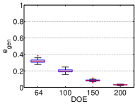
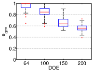
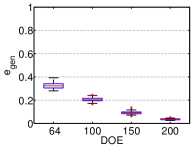
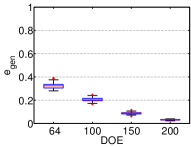
Figure 10 displays the results associated with the O’Hagan function. Similarly to the Morris function, the performance of PC-Kriging in the case of the O’Hagan function resembles that of ordinary Kriging whereas PCE performs worse than the other three approaches. Over the entire displayed range of experimental designs in Fig. 10, the performance of OPC-Kriging is slightly better than the performance of SPC-Kriging and ordinary Kriging. Note that meta-modeling the O’Hagan function requires less samples in the experimental design to obtain the same accuracy as in the case of the Rastrigin function despite the fact that the O’Hagan function has a 15-dimensional input space and that both functions are very smooth.
Summarizing the results of all six analytical functions in Fig. 5-10, the proposed PC-Kriging approaches perform better than or at least as good as the traditional PCE and Kriging approaches. Note that for functions like O’Hagan (Fig. 10) and Morris (Fig. 8) the performance of PC-Kriging is more similar to Kriging than PCE, whereas for the other functions the performance of PC-Kriging resembles more that of PCE. As one could expect, there is no general rule so as to decide whether PCE or Kriging provide the most accurate meta-models for a given experimental design. The advantage of PC-Kriging is to perform as least as well as the best of the two.
The combination of PCE and Kriging and its increased accuracy comes with a higher computational cost. The traditional ordinary Kriging and PCE approaches have the lowest computational cost, SPC-Kriging has an intermediate and OPC-Kriging has the highest cost. The high cost of OPC-Kriging originates from the iterative character of the algorithm and the accompanying repetitive calibration of Kriging models. OPC-Kriging computes LAR and calibrates Kriging models with increasing complex trend, whereas ordinary Kriging consists of a single calibration of a Kriging model with constant trend. For a single calibration of a surrogate of the Ishigami function (experimental design of size samples) the ratio of computational times when comparing PCE to ordinary Kriging, SPC-Kriging and OPC-Kriging is approximately , and , respectively.
Note that it is intended to apply these techniques to realistic problems where the evaluation of the exact computational model response lasts much longer than the computation of a meta-model. The apparent computational overload of OPC-Kriging will not be anymore an issue in many practical applications.
5.3.3 Large experimental designs
When the resources for experiments are limited the focus lies on doing as few computational model runs as possible as discussed in the previous section. In order to describe the entire behavior of the meta-modeling approaches, the Ishigami function is also studied now for larger experimental designs in order to assess the convergence of the various schemes. Results are shown in Fig. 11. This figure illustrates the evolution of the relative generalization error from small to large sample sizes on the logarithmic (base 10) scale. The error measure decreases fast when enlarging the sample set because the Ishigami function is composed of sine and cosine functions which can be approximated well with series of polynomials, e.g. as in a Taylor expansion. Thus PCE is the dominating effect for PC-Kriging.
For large sample sizes, ordinary Kriging is outperformed by the other three approaches. Kriging in general works well with small sample sizes. If too many samples are used, the interpolation algorithm becomes unstable due to singularities and bad conditioning in the auto-correlation matrix. If a large sample size is available, regional Kriging models on a subset of samples, e.g. the neighboring samples, are more suitable Dubrule (1983).
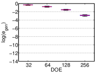
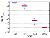
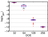
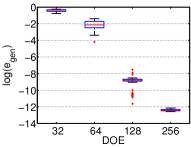
The performance of PC-Kriging and also PCE for a large number of samples (here 128 and 256 samples in Fig. 11) is in the order of magnitude of the machine computation precision. Errors around originate from numerical round-off errors which are not reducible by adding more samples. It is questionable though, whether in reality such a high accuracy in the meta-model prediction is needed.
5.3.4 Evolution of the error measures
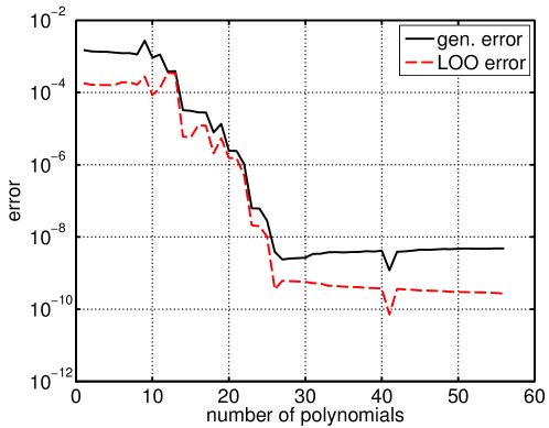
The OPC-Kriging algorithm includes the tracking of the LOO error to optimally choose the sparse set of orthonormal polynomials. The evolution of the LOO error for the Ishigami function and a sample size of samples is presented in Fig. 12. The experimental-design-based LOO error (dashed, red line) is compared to the relative generalization error which is shown as the solid black line.
The first point to notice is that the LOO error slightly under-predicts the true value of the relative generalization error for all sizes of polynomial sets. This is due to the fact that the LOO error is based solely on the information contained in the experimental design samples whereas the relative generalization error is based on a large validation set (). Although there is an inherent under-prediction, the overall behavior of the two error measures is similar. Thus the choice of the optimal set of polynomials for the OPC-Kriging can be based on the LOO error, which is obtained as a by-product of the procedure used to fit the parameters of the PC-Kriging model. In the example case of Fig. 12, choosing only half of the polynomials, i.e. leads to a meta-model which is almost as accurate as using all polynomials. The optimal set of polynomials can be chosen at the point where the decrease in LOO error becomes insignificant. This reduces the number of polynomials needed and thus also reduces the complexity of the OPC-Kriging meta-model.
6 Conclusion
In the context of increasing computational power, computational models in engineering sciences have become more and more complex. Many analyses such as reliability assessment or design optimization, require repeated runs of such computational models which may be infeasible due to resource limitations. To overcome these limitations computational models are nowadays approximated by easy-to-evaluate functions called meta-models.
This paper summarized the principles of two popular non-intrusive meta-modeling techniques, namely Polynomial Chaos Expansions (PCE) and Kriging (also called Gaussian process modeling). Then the combination of the two approaches to a new meta-modeling approach called Polynomial-Chaos-Kriging (PC-Kriging) is proposed. Two formulations of PC-Kriging are introduced in this paper, namely Optimal-PC-Kriging (OPC-Kriging) and Sequential-PC-Kriging (SPC-Kriging). SPC-Kriging employs first a least-angle-regression (LAR) algorithm to determine the optimal sparse set of orthonormal polynomials in the input space. Then, the set of polynomials is used as the trend of a universal Kriging meta-model. OPC-Kriging employs the same least-angle-regression algorithm as SPC-Kriging, yet iteratively adds polynomials to the trend part of the universal Kriging model one-by-one, and fit the hyperparameters of the auto-correlation function in each iteration. In this case polynomials are added to the trend in the order they are selected by the LAR algorithm. Based on the LOO error the best meta-model is found to be the OPC-Kriging meta-model.
The performance of the four approaches (ordinary Kriging, PCE, SPC-Kriging, OPC-Kriging) is compared in terms of the relative generalization error on benchmark analytical functions. The results show that PC-Kriging is better than, or at least as good as the distinct approaches for small experimental designs. Specifically, OPC-Kriging is preferable to SPC-Kriging as it reduces the number of polynomials in the regression part and thus reduces the complexity of the meta-model, at a computational calibration cost which is however higher than that of SPC-Kriging.
The analysis of the performance of PC-Kriging is limited to some benchmark analytical functions in this paper. The ongoing research applies PC-Kriging to realistic engineering problems such as reliability analysis or design optimization. The idea of adaptive experimental designs (also called design enrichment) is introduced in order to increase the accuracy of the surrogate in some specific regions of the input space (e.g. close to the zero-level of the limit state function in reliability analysis) instead of everywhere. The initialization of the iterative algorithm is a small initial experimental design to which points are added in regions of interest. These added points will then increase the quality of the meta-model specifically in those regions. Preliminary ideas developed in Schöbi and Sudret (2014b, c, a) are currently investigated in details.
Acknowledgements
This research was carried out with the support of Orange Labs, Issy-les-Moulineaux, France under the research agreement #C12063. This support is gratefully acknowledged.
References
- Allen (1971) Allen, D. (1971). The prediction sum of squares as a criterion for selecting predictor variables. Technical Report 23, Tech. Rep. 23, Dept. of Statistics, University of Kentucky.
- Bachoc (2013a) Bachoc, F. (2013a). Asymptotic analysis of the role of spatial sampling for hyper-parameter estimation of Gaussian processes. arXiv:1301.4321.
- Bachoc (2013b) Bachoc, F. (2013b). Cross validation and maximum likelihood estimations of hyper-parameters of Gaussian processes with model misspecifications. Comput. Stat. Data Anal. 66, 55–69.
- Bachoc et al. (2014) Bachoc, F., G. Bois, J. Garnier, and J.-M. Martinez (2014). Calibration and improved prediction of computer models by universal Kriging. Nucl. Sci. Eng. 176, 91–97.
- Bect et al. (2012) Bect, J., D. Ginsbourger, L. Li, V. Picheny, and E. Vazquez (2012). Sequential design of computer experiments for the estimation of a probability of failure. Stat. Comput. 22, 773–793.
- Berveiller et al. (2006a) Berveiller, M., B. Sudret, and M. Lemaire (2006a). A stochastic finite element procedure for moment and reliability analysis. Eur. J. Comput. Mech. 15(7-8), 825–866.
- Berveiller et al. (2006b) Berveiller, M., B. Sudret, and M. Lemaire (2006b). Stochastic finite elements: a non intrusive approach by regression. Eur. J. Comput. Mech. 15(1-3), 81–92.
- Bichon et al. (2011) Bichon, B., J. McFarland, and S. Mahadevan (2011). Efficient surrogate models for reliability analysis of systems with multiple failure modes. Reliab. Eng. Sys. Safety 96(10), 1386–1395.
- Bichon et al. (2008) Bichon, B. J., M. S. Eldred, L. Swiler, S. Mahadevan, and J. McFarland (2008). Efficient global reliability analysis for nonlinear implicit performance functions. AIAA J. 46(10), 2459–2468.
- Blatman (2009) Blatman, G. (2009). Adaptive sparse polynomial chaos expansions for uncertainty propagation and sensitivity analysis. Ph. D. thesis, Université Blaise Pascal, Clermont-Ferrand.
- Blatman and Sudret (2008) Blatman, G. and B. Sudret (2008). Sparse polynomial chaos expansions and adaptive stochastic finite elements using regression approach. Comptes Rendus Mécanique 336, 518–523.
- Blatman and Sudret (2010a) Blatman, G. and B. Sudret (2010a). An adaptive algorithm to build up sparse polynomial chaos expansions for stochastic finite element analysis. Prob. Eng. Mech. 25(2), 183–197.
- Blatman and Sudret (2010b) Blatman, G. and B. Sudret (2010b). Efficient computation of global sensitivity indices using sparse polynomial chaos expansions. Reliab. Eng. Sys. Safety 95, 1216–1229.
- Blatman and Sudret (2011) Blatman, G. and B. Sudret (2011). Adaptive sparse polynomial chaos expansion based on Least Angle Regression. J. Comput. Phys 230, 2345–2367.
- Byrd et al. (1999) Byrd, R. H., M. E. Hribar, and J. Nocedal (1999). An interior point algorithm for large-scale nonlinear programming. SIAM J. Optim. 9(4), 877–900.
- Chkifa et al. (2013) Chkifa, A., A. Cohen, G. Migliorati, F. Nobile, and R. Tempone (2013). Discrete least squares polynomial approximation with random evaluations - appliations to parametric and stochastic elliptic PDEs. Technical report, MATHICSE, EPFL, Lausanne, Switzerland.
- Choi et al. (2004) Choi, S. K., R. V. Grandhi, R. A. Canfield, and C. L. Pettit (2004). Polynomial chaos expansion with Latin Hypercube sampling for estimating response variability. AIAA J. 45, 1191–1198.
- Clarke et al. (2003) Clarke, S. M., J. H. Griebsch, and T. W. Simpson (2003). Analysis of support vector regression for approximation of complex engineering analyses. In Proc. DETC’03, Des. Eng. Tech. Conf. Comput. Inf. Eng. Conf. Chicago.
- De Rocquigny et al. (2008) De Rocquigny, E., N. Devictor, and S. Tarantola (Eds.) (2008). Uncertainty in industrial practice – A guide to quantitative uncertainty management. John Wiley & Sons.
- Deng et al. (2013) Deng, W., X. Yang, L. Zou, M. Wang, Y. Liu, and Y. Li (2013). An improved self-adaptive differential evolution algorithm and its application. Chemometrr. Intell. Lab. 128, 66–76.
- Doostan and Owhadi (2011) Doostan, A. and H. Owhadi (2011). A non-adapted sparse approximation of pdes with stochastic inputs. J. Comput. Phys. 230(8), 3015–3034.
- Doostan et al. (2013) Doostan, A., A. Validi, and G. Iaccarino (2013). Non-intrusive low-rank separated approximation of high-dimensional stochastic models. Comput. Methods Appl. Mech. Eng. 263, 42–55.
- Dubourg (2011) Dubourg, V. (2011). Adaptive surrogate models for reliability analysis and reliability-based design optimization. Ph. D. thesis, Université Blaise Pascal, Clermont-Ferrand, France.
- Dubourg and Sudret (2014) Dubourg, V. and B. Sudret (2014). Meta-model-based importance sampling for reliability sensitivity analysis. Structural Safety 49, 27–36.
- Dubourg et al. (2011) Dubourg, V., B. Sudret, and J. M. Bourinet (2011). Reliability-based design optimization using Kriging and subset simulation. Struct. Multidisc. Optim. 44(5), 673–690.
- Dubourg et al. (2013) Dubourg, V., B. Sudret, and F. Deheeger (2013). Metamodel-based importance sampling for structural reliability analysis. Prob. Eng. Mech. 33, 47–57.
- Dubrule (1983) Dubrule, O. (1983). Cross validation of Kriging in a unique neighbourhood. Math. Geol. 15(6), 687–698.
- Durrande et al. (2012) Durrande, N., D. Ginsbourger, and O. Roustant (2012). Additive covariance kernels for high-dimensional Gaussian process modeling. Ann. Fac. Sci. Toulouse Tome 21 3, 481–499.
- Durrande et al. (2013) Durrande, N., D. Ginsbourger, and O. Roustant (2013). ANOVA kernels and RKHS of zero mean function for model-based sensitivity analysis. J. Multivar. Anal. 115, 57–67.
- Duvenaud et al. (2011) Duvenaud, D. K., H. Nickisch, and C. E. Rasmussen (2011). Additive gaussian processes. In J. Shawe-Taylor, R. Zemel, P. Bartlett, F. Pereira, and K. Weinberger (Eds.), Advances in Neural Information Processing Systems 24, pp. 226–234. Curran Associates, Inc.
- Echard et al. (2011) Echard, B., N. Gayton, and M. Lemaire (2011). AK-MCS: an active learning reliability method combining kriging and Monte Carlo simulation. Structural Safety 33(2), 145–154.
- Echard et al. (2013) Echard, B., N. Gayton, M. Lemaire, and N. Relun (2013). A combined importance sampling and Kriging reliability method for small failure probabilities with time-demanding numerical models. Reliab. Eng. Syst. Safety 111, 232–240.
- Efron et al. (2004) Efron, B., T. Hastie, I. Johnstone, and R. Tibshirani (2004). Least angle regression. Ann. Stat. 32, 407–499.
- Eldred (2009) Eldred, M. S. (2009). Recent advances in non-intrusive polynomial chaos and stochastic collocation methods for uncertainty analysis and design. In 50th AIAA/ASME/ASCE/AHS/ASC Struct. Struct. Dyn. Mater. Conf.
- Eldred et al. (2008) Eldred, M. S., C. G. Webster, and P. G. Constantine (2008). Design under uncertainty employing stochastic expansion methods. In Proc. 12th AIAA/ISSMO Multidiscip. Anal. Optim. Conf. Victoria, British Columbia, Canada.
- Fletcher (1970) Fletcher, R. (1970). A new approach to variable metric algorithms. Comput. J. 13, 317–322.
- Forrester et al. (2008) Forrester, A., A. Sóbester, and A. Keane (2008). Engineering design via surrogate modelling. Wiley.
- Geisser (1975) Geisser, S. (1975). The predictive sample reuse method with applications. J. Amer. Stat. Assoc. 70, 320–328.
- Ghanem and Spanos (2003) Ghanem, R. and P. Spanos (2003). Stochastic Finite Elements : A Spectral Approach (2nd ed.). Courier Dover Publications, Mineola.
- Ghiocel and Ghanem (2002) Ghiocel, D. and R. Ghanem (2002). Stochastic finite element analysis of seismic soil-structure interaction. J. Eng. Mech. 128, 66–77.
- Ginsbourger et al. (2013) Ginsbourger, D., N. Durrande, and O. Roustant (2013). Kernels and designs for modelling invariant functions: From group invariance to additivity. Technical Report hal-00731657, INRIA.
- Ginsbourger et al. (2013) Ginsbourger, D., O. Roustant, and N. Durrande (2013, August). Invariances of random fields paths, with applications in Gaussian Process Regression. arXiv:1308.1359.
- Goldberg (1989) Goldberg, G. H. (1989). Genetic Algorithms in Search, Optimization, and Machine Learning. Addison-Wesley Professional.
- Goldfarb (1970) Goldfarb (1970). A Family of Variable-Metric Methods Derived by Variational Means. Math. Comput. 24, 23–26.
- Gunn (1998) Gunn, S. R. (1998). Support vector machines for classification and regression. Technical Report ISIS-1-98, Dpt. of Electronics and Computer Science, University of Southampton.
- Hastie et al. (2001) Hastie, T., R. Tibshirani, and J. Friedman (2001). The elements of statistical learning: Data mining, inference and prediction. Springer, New York.
- Jakeman et al. (2014) Jakeman, J. D., M. S. Eldred, and K. Sargsyan (2014). Enhancing -minimization estimates of polynomial chaos expansions using basis selection. arXiv:1407.8093, 1–26.
- Jones et al. (1998) Jones, D. R., M. Schonlau, and W. J. Welch (1998). Efficient global optimization of expensive black-box functions. J. Glob. Optim. 13(4), 455–492.
- Kaymaz (2005) Kaymaz, I. (2005). Application of kriging method to structural reliability problems. Structural Safety 27(2), 133–151.
- Keese and Matthies (2005) Keese, A. and H. G. Matthies (2005). Hierarchical parallelisation for the solution of stochastic finite element equations. Comp. Struct. 83, 1033–1047.
- Krige (1951) Krige, D. G. (1951). A statistical approach to some basic mine valuation problems on the Witwatersrand. J. Chem. Metall. Mining Soc. South Africa 52(6), 119–139.
- Le Maître et al. (2002) Le Maître, O. P., M. Reagan, H. N. Najm, R. G. Ghanem, and O. M. Knio (2002). A stochastic projection method for fluid flow – II. Random process. J. Comput. Phys. 181, 9–44.
- Lophaven et al. (2002) Lophaven, S., H. B. Nielsen, and J. Sø ndergaard (2002). DACE, A Matlab Kriging Toolbox.
- Marrel et al. (2008) Marrel, A., B. Iooss, F. Van Dorpe, and E. Volkova (2008). An efficient methodology for modeling complex computer codes with Gaussian processes. Comput. Stat. Data Anal. 52, 4731–4744.
- Matérn (1986) Matérn, B. (1986). Spatial variation. Lect. Notes Stat. 36.
- McKay et al. (1979) McKay, M. D., R. J. Beckman, and W. J. Conover (1979). A comparison of three methods for selecting values of input variables in the analysis of output from a computer code. Technometrics 2, 239–245.
- Migliorati et al. (2014) Migliorati, G., F. Nobile, E. von Schwerin, and R. Tempone (2014, March). Analysis of discrete L2 projection on polynomial spaces with random evaluations. Found. Comput. Math. 14(3), 419–456.
- Morris (1991) Morris, M. D. (1991). Factorial sampling plans for preliminary computational experiments. Technometrics 33(2), 161–174.
- Oakley and O’Hagan (2004) Oakley, J. and A. O’Hagan (2004). Probabilistic sensitivity analysis of complex models: a Bayesian approach. J. R. Stat. Soc., Ser. B 66, 751–769.
- Peng et al. (2014) Peng, J., J. Hampton, and A. Doostan (2014). A weighted-minimization approach for sparse polynomial chaos expansions. J. Comput. Phys..
- Rasmussen and Williams (2006) Rasmussen, C. E. and C. K. I. Williams (2006). Gaussian processes for machine learning. Adaptive computation and machine learning. Cambridge, Massachusetts: MIT Press.
- Rastrigin (1974) Rastrigin, L. (1974). Systems of extremal control. Zinatne, Riga.
- Rosenbrock (1960) Rosenbrock, H. (1960). An automatic method for finding the greatest or least value of a function. Comput. J. 3, 175–184.
- Roustant et al. (2012) Roustant, O., D. Ginsbourger, and Y. Deville (2012). DiceKriging, DiceOptim: Two R package for the analysis of computer experiments by Kriging-based metamodeling and optimisation. J. Stat. Software 51, 1–55.
- Roustant et al. (2013) Roustant, O., D. Ginsbourger, and Y. Deville (2013). Package DiceKriging - Kriging methods for computer experiments.
- Sacks et al. (1989) Sacks, J., W. J. Welch, T. J. Mitchell, and H. P. Wynn (1989). Design and analysis of computer experiments. Stat. Sci. 4, 409–435.
- Santner et al. (2003) Santner, T. J., B. J. Williams, and W. I. Notz (2003). The design and analysis of computer experiments. Springer series in Statistics. Springer.
- Saporta (2006) Saporta, G. (2006). Probabilités, analyse des données et statistique. Technip.
- Sarangi et al. (2014) Sarangi, S., K. K. Bodla, S. V. Garimella, and J. Y. Murthy (2014). Manifold microchannel heat sink design using optimization under uncertainty. Int. J. Heat Mass Tran. 69, 92–105.
- Sargsyan et al. (2014) Sargsyan, K., C. Safta, H. Najm, B. Debusschere, D. Ricciuto, and P. Thornton (2014). Dimensionality reduction for complex models via Bayesian compressive sensing. Int. J. Unc. Quant. 4, 63–94.
- Schöbi and Sudret (2014a) Schöbi, R. and B. Sudret (2014a). Combining polynomial chaos expansions and Kriging for solving structural reliability problems. In P. Spanos and G. Deodatis (Eds.), Proc. 7th Int. Conf. on Comp. Stoch. Mech (CSM7), Santorini, Greece.
- Schöbi and Sudret (2014b) Schöbi, R. and B. Sudret (2014b). PC-Kriging: A new meta-modelling method and its applications to quantile estimation. In J. Li and Y. Zhao (Eds.), Proc. 17th IFIP WG7.5 Conference on Reliability and Optimization of Structural Systems, Huangshan, China. Taylor & Francis.
- Schöbi and Sudret (2014c) Schöbi, R. and B. Sudret (2014c). PC-Kriging: a new metamodelling method combining polynomial chaos expansions and Kriging. In Proc. 2nd Int. Symposium on Uncertainty Quantification and Stochastic Modeling, Rouen, France.
- Shanno (1970) Shanno, D. F. (1970). Conditioning of quasi-Newton methods for function minimization. Math. Comput. 24, 647–656.
- Smola and Schölkopf (2006) Smola, A. J. and B. Schölkopf (2006). A tutorial on support vector regression. Stat. Comput. 14, 199–222.
- Sobol’ (1993) Sobol’, I. M. (1993). Sensitivity estimates for nonlinear mathematical models. Math. Model. Comp. Exp. 1, 407–414.
- Soize and Ghanem (2004) Soize, C. and R. Ghanem (2004). Physical systems with random uncertainties: chaos representations with arbitrary probability measure. SIAM J. Sci. Comput. 26(2), 395–410.
- Stein (1999) Stein, M. L. (1999). Interpolation of spatial data: some theory for Kriging. Springer-Verlag, New York.
- Stone (1974) Stone, M. (1974). Cross-validatory choice and assessment of statistical predictions. J. R. Stat. Soc., Ser. B 36, 111–147.
- Storlie et al. (2009) Storlie, C. B., L. P. Swiler, J. C. Helton, and C. J. Sallaberry (2009). Implementation and evaluation of nonparametric regression procedures for sensitivity analysis of computationally demanding models. Reliab. Eng. Sys. Safety 94, 1735–1763.
- Storn and Price (1997) Storn, R. and K. Price (1997). Differential evolution, a simple and efficient heuristic for global optimization over continuous spaces. J. Global Optim. 11(4), 341–359.
- Sudret (2007) Sudret, B. (2007). Uncertainty propagation and sensitivity analysis in mechanical models – contributions to structural reliability and stochastic spectral methods. Technical report. Habilitation à diriger des recherches, Université Blaise Pascal, Clermont-Ferrand, France (229 pages).
- Sudret (2008) Sudret, B. (2008). Global sensitivity analysis using polynomial chaos expansions. Reliab. Eng. Syst. Safety 93(7), 964–979.
- Sudret (2014) Sudret, B. (2014). Polynomials chaos expansions and stochastic finite element methods. In J. Phoon, K.-K. and Ching (Ed.), Risk Reliab. Geotech. Eng., Chapter 5. Taylor and Francis.
- Sudret et al. (2004) Sudret, B., M. Berveiller, and M. Lemaire (2004). Eléments finis stochastiques en élasticité linéaire. Comptes Rendus Mecanique 332(7), 531–537.
- Tibshirani (1996) Tibshirani, R. (1996). Regression shrinkage and selection via LASSO. J. Roy. Stat. Soc. B 58, 267–288.
- Vapnik (1995) Vapnik, V. (1995). The nature of statistical learning theory. Springer.
- Vazquez and Walter (2003) Vazquez, E. and E. Walter (2003). Multi-output support vector regression. In Proc. 13th IFAC Symp. Syst. Identification, Rotterdam, pp. 1820–1825.
- Wan and Karniadakis (2006) Wan, X. and G. Karniadakis (2006). Beyond Wiener-Askey expansions: handling arbitrary PDFs. J. Sci. Comput. 27, 455–464.
- Wan and Karniadakis (2005) Wan, X. and G. E. Karniadakis (2005). An adaptive multi-element generalized polynomial chaos method for stochastic differential equations. J. Comput. Phys. 209, 617–642.
- Xiu (2009) Xiu, D. (2009). Fast numerical methods for stochastic computations: a review. Comm. Comput. Phys. 5(2-4), 242–272.
- Xiu and Hesthaven (2005) Xiu, D. and J. S. Hesthaven (2005). High-order collocation methods for differential equations with random inputs. SIAM J. Sci. Comput. 27(3), 1118–1139.
- Xiu and Karniadakis (2002) Xiu, D. and G. E. Karniadakis (2002). The Wiener-Askey polynomial chaos for stochastic differential equations. SIAM J. Sci. Comput. 24(2), 619–644.