Overlapping non Matching Meshes Domain Decomposition Method in Isogeometric Analysis

Abstract

One of the important aspects of IsoGeometric Analysis (IGA) is its link to Computer Aided Design (CAD) geometry methods. Two of IGA’s major challenges are geometries made of boolean assemblies such as in Constructive Solid Geometry (CSG), and local refinements. In the present work we propose to apply the Additive Schwarz Domain Decomposition Method (ASDDM) on overlapping domains to actually solve Partial Differential Equations (PDEs), on assemblies as well as a means for local refinement.

As a first step we study a collection of simple two domains problems, using the software package GeoPDEs, all of them converged rapidly, even on very distorted domains. For local refinement we implement a ”Chimera” type of zooming together with ASDDM iterations, and here again we get very attractive results. A last effect is that the additive methods are naturally parallelizable and thus can extend to large 3D problems. We give some examples of computations on multi-patch bodies.

This new implementation of the DD methods brings many interesting problems such as: the definition of boundary conditions on trimmed patches, choice of blending operators on the intersections , optimization of the overlap size, choice of preconditionning to guarantee convergence ( as we do not have a maximum principle here.)

1 Motivation: Using IsoGeometry and Domain Decomposition Methods Together

One of the main purposes of Constructive Solid Geometry is to provide CAD with the tools allowing the engineer to perform Boolean operations on the bodies he works with. There are very many engineering forms which are obtained as unions, intersections, subtractions etc. of basic geometrical figures, see Figure 1 for example. Even quite complicated bodies can often be represented as results of such set operations applied to some primitive geometrical forms like cubes, balls, cylinders etc. [18]. To solve Partial differential equations on domains defined by such solids , it seems natural to find methods that take advantage of the definitions of such solids.

IsoGeometric Analysis (IGA)  [14] is a relatively new numerical method of solving PDEs, derived from the FEM. The main features of IGA, which are very important in engineering and which FEM lacks, are: (1) exact representation of the geometry and (2) the same family of basis functions that are used in the construction of the geometry are used in the solution of PDEs, thus avoiding the cumbersome mesh generation step.

The main concept of IGA can be described in the following way. Assume that we work in 3-dimensional environment and consider a cube, which constitutes the reference space. The geometrical domain is build as a continuous deformation of the reference cube, as shown in Figure  2, and represents the exact geometrical form. Given a finite space of basis functions on the reference domain we apply the geometrical mapping to them to generate the finite space of solutions, as the space spanned by their images.

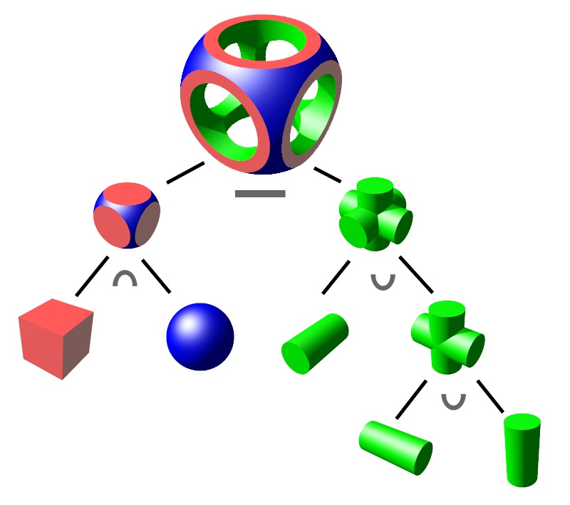
Figure 1: CSG example of Boolean operations.

Since a single patch is limited, one would like to extend IGA to complex domainss, and based on CSG and consider a collection of subdomains . Domain Decomposition (DD) methods are then natural candidates for the solution of PDEs over complex domains. More for IGA the problem of local zooming becomes more involved since the refinement need to be introduced at the level of the parametric space, where the rigid structure of tensor product must be respected.( In view of this restriction different methods of local zooming were proposed for IGA. Popular ways of doing that is the T-spline technique  [20] or the Truncated Hierarchical B Splines (THB) one,  [10]. This allows one to locally refine the mesh, but still the tensor product structure of the parametric space leads to non-local changes in the mesh  [8], implying that many additional degrees of freedom are introduced around the areas being magnified, and increasing the computational costs of the solution. ). Domain Decomposition (DD) methods, can also bring a solution here by using local zooming or Chimera type methods introduced in Dougherty at all  [9].

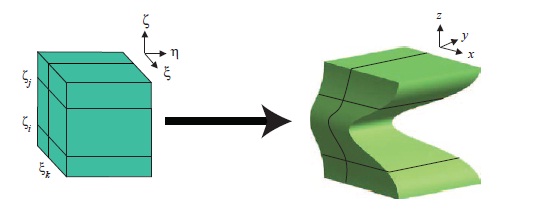
Figure 2: An example of IsoGeometric mapping.

Domain Decomposition partitions the original domain into a set of overlapping( or just glued together) connected subdomains with smooth boundary and then solve the PDEs on each of them iteratively, see  [1] for a detailed exposition. In most implementations the meshes of contiguous domains match or are linked by a mortar element. It has been studied for IGA in  [3] and  [16].

In the present work we introduce the definition and properties of DD methods for non-matching meshes over overlapping subdomain meshes as well as applications to problems of local refinement (zooming) . For zooming the meshes of the newly constructed subdomains are independently defined and non-matching , but the geometry of the whole domain is unchanged. This way of solving the local zooming problem allows us to introduce new degrees of freedom only in the region under investigation, at the same time we use the IGA framework with all its advantages.

2 Overview of this work

In the next part we recall some definitions and notations related to B-splines, which are the cornerstones of all the IGA technique. We consider the refinement procedures such as knot insertion and degree elevation, which allow us to introduce local refinement and zooming to the IGA.

As a model example we state the classical Poisson equation in its continuous form. We then proceed to the weak form of this problem, which gives us quite a natural way of solving the equation numerically, the Galerkin method, used in FEM and IGA. Then the main ideas of IGA are explained with all the computations needed to perform the actual calculations of the approximate solution. Imposing non homogeneous Dirichlet boundary conditions is not straight forward in IGA and some special techniques should be used to impose them. We describe two different methods for imposing essential boundary conditions.

The next part introduces the family of Schwarz Domain Decomposition methods and gives their description. We choose to implement the Additive Schwarz Domain Decomposition Method (ASDDM), that is equivalent to a block Jacobi iterative process since it may be easily parallelized and we detail its continuous and discretized weak forms.

In the sixth part the Discretized Schwarz Domain Decomposition Method is described. The construction of exact and approximation projection operators for the imposition of Dirichlet boundary conditions is treated.

The next part illustrates the Schwarz Algorithm in the one-dimensional case. We give the detailed overview of the matrix operator forms obtained from the ASDDM.

We then give numerous numerical results. Based on the GeoPDEs software  [4], we have developed a code that implements the ASDDM using IGA and applied it to solve different one-, two-, and three-dimensional problems. In this section all the convergence results are provided. We also describe how the code was parallelized and show three-dimensional examples, computed by it.

We conclude by discussing further directions for this research and open problems.

3 B-splines

3.1 Introduction

The most popular geometrical forms being used in CAGD are based on B-splines. Their definition provides us with very important geometrical properties. In particular, the degree of a B-spline curve is strictly related to the number of control points and they give us local control over the form of the curve. B-splines are not general enough to describe exactly even very simple shapes such as cylinders, balls, circles, etc. The notion of Non - Uniform Rational B-Splines (NURBS) extends B-splines and allows one to exactly represent a wide array of objects that cannot be exactly represented by polynomials, many of which are ubiquitous in engineering design. In the present work we will consider only B-Splines .We will now provide the exact definitions. All the details can be found in  [19].

3.2 B-spline basis functions

Let $\Xi$ be a set of $m$ non-decreasing numbers, $\xi_{1}\leq\xi_{1}\leq\xi_{2}\leq\dots\leq\xi_{m}$. The $\xi_{i}$’s are called knots, the set $\Xi$ is the knot vector, and the half-open interval $[\xi_{i},\xi_{i+1})$ is the $i$-th knot span. If a knot $\xi_{i}$ appears $k$ times (i.e., $\xi_{i}=\xi_{i+1}=\dots=\xi_{i+k-1}$), where $k>1$, $\xi_{i}$ is a multiple knot of multiplicity $k$ and the corresponding knot span does not exist. Otherwise, if $\xi_{i}$ appears only once, it is a simple knot. If the knots are equally spaced, the knot vector or the knot sequence is said to be uniform; otherwise, it is non-uniform.

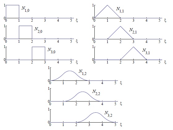
Figure 3: B-spline basis functions of order 0, 1 and 2 for uniform knot vector $\Xi=[0,1,2,3,\dots]$.

To define B-spline basis functions, we need one more parameter, the degree of these basis functions, $p$. The $i$-th B-spline basis function of degree $p$, written as $N_{i,p}(\xi)$, is defined recursively as follows:

$$N_{i,0}=\left\{\begin{array}[]{l l}1&\quad\text{if $\xi_{i}\leq\xi<\xi_{i+1}$,}\\ 0&\quad\text{otherwise.}\\ \end{array}\right.$$ (3.2.1)

$$N_{i,p}(\xi)=\frac{\xi-\xi_{i}}{\xi_{i+p}-\xi_{i}}N_{i,p-1}(\xi)+\frac{\xi_{i+p+1}-\xi}{\xi_{i+p+1}-\xi_{i+1}}N_{i+1,p-1}(\xi).$$ (3.2.2)

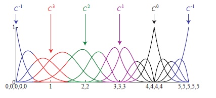
Figure 4: Quartic $(p=4)$ basis functions for an open, non-uniform knot vector $\Xi=[0,0,0,0,0,1,2,2,3,3,3,4,4,4,4,5,5,5,5,5]$. The continuity across an interior element boundary is a direct result of the polynomial order and the multiplicity of the corresponding knot value.

If the degree is zero (i.e., $p=0$), these basis functions are all indicators of the the intervals they are defined on.

In general, basis functions of order $p$ have $p-k$ continuous derivatives across knot $\xi_{i}$, where $k$ is the multiplicity of the value $\xi_{i}$ as before. When the multiplicity of a knot value is exactly $p$, the basis is interpolatory at that knot. When the multiplicity is $p+1$, the basis becomes discontinuous; the patch boundaries are formed in this way.

3.3 B-spline curves

In order to define a B-spline we have to provide the following information: a set of $n$ control points $\{P_{i}\}_{i=1}^{n}$, a knot vector $\Xi=\{\xi_{i}\}_{i=1}^{m}$ of $m$ knots, and a degree $p$, such that $n$, $m$ and $p$ must satisfy $m=n+p+1$.

Given this information the B-spline curve of degree $p$ defined by these control points and knot vector $\Xi$ is

$$\mathbf{C}(\xi)=\sum_{i=1}^{n}N_{i,p}(\xi)\mathbf{P}_{i},$$

where $N_{i,p}(u)$’s are the B-spline basis functions of degree $p$.

The point on the curve that corresponds to a knot $\xi_{i}$, $C(\xi_{i})$, is referred to as a knot point. Hence, the knot points divide a B-spline curve into curve segments, each of which is defined on a knot span.

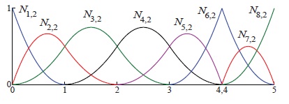
Figure 5: Quadratic basis functions for open, non-uniform knot vector $\Xi=\{0,0,0,1,2,3,4,4,5,5,5\}$

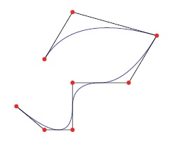
Figure 6: An example of a B-spline curve and its control points

If the knot vector does not have any particular structure, the generated curve will not touch the first and last legs of the control polygon. This type of B-spline curves is called open B-spline curves. In order to make the curve interpolatory the first knot and the last knot must be of multiplicity $p+1$. By repeating the first and the last knots $p+1$ times the curve starts at $P_{0}$ and ends at $P_{n}$. A knot vector of such form is called an open knot vector. Here we consider all the knot vectors to be open if we don’t state otherwise (e.g., it is not the case when periodic NURBS are discussed).

In Figure  6 you can see an example of a B-spline curve. We chose a non-uniform knot vector $\Xi=\{0,0,0,1,2,3,4,4,5,5,5\}$ and the control points as shown in the figure. The corresponding parametric space and the B-spline basis functions are shown in Figure  5.

3.4 Derivatives of B-spline

Since the B-spline basis functions are obtained by recursion from the lower degree B-spline basis functions and the dependence is linear, we can obtain the recursive formulas for their derivatives in a similar way and represent them as a linear combination of B-spline basis functions of lower degrees, see  [19].

The derivative of a basis function is given by

$$N^{\prime}{}_{i,p}(\xi)=\frac{p}{\xi_{i+p}-\xi_{i}}N_{i,p-1}(\xi)-\frac{p}{\xi_{i+p+1}-\xi_{i+1}}N_{i+1,p-1}(\xi).$$ (3.4.1)

The proof of this recurrence is obtained by induction on $p$.

It is a little more complicated task to calculate the NURBS derivatives since they are fractions of linear combinations of the B-spline basis functions, but still the recurrence relation exists and may be found in the Appendix.

3.5 Multi-dimensional B-splines

All the definitions given above refer to curves. One can easily extend these definitions to surfaces and bodies by taking a tensor product of an appropriate number of knot vectors and defining the basis functions as the products of the corresponding one-dimensional basis functions. More exactly, given a control net $\{\mathbf{P}_{i,j}\}_{i,j=1}^{n,m}$, polynomial orders $p$ and $q$, and knot vectors $\Xi=\{\xi_{i}\}_{i=1}^{n+p+1}$ and $\Upsilon=\{\upsilon_{i}\}_{i=1}^{m+q+1}$, a tensor product B-spline surface is defined by

$$\mathbf{S}(\xi,\upsilon)=\sum_{i=1}^{n}\sum_{j=1}^{m}N_{i,p}(\xi)M_{j,q}(\upsilon)\mathbf{P}_{i,j},$$ (3.5.1)

where $N_{i,p}(\xi)$ and $M_{j,q}(\upsilon)$ are the univariate B-spline basis functions corresponding to knot vectors $\Xi$ and $\Upsilon$, respectively.

Many of the properties of a B-spline surface are the result of its tensor product nature. The basis functions are point-wise nonnegative, and form a partition of unity as for any $(\xi,\upsilon)\in[\xi_{1},\xi_{n+p+1}]\times[\upsilon_{1},\upsilon_{m+q+1}],$

$$\sum_{i=1,j=1}^{n,m}N_{i,p}(\xi)M_{j,q}(\upsilon)=\left(\sum_{i=1}^{n}N_{i,p}(\xi)\right)\left(\sum_{j=1}^{m}M_{j,q}(\upsilon)\right)=1.$$

The local support of the basis functions also follows directly from the one-dimensional functions that form them. The support of a given bivariate function $\widetilde{N}_{i,j;p,q}(\xi,\upsilon)=N_{i,p}(\xi)M_{j,q}(\upsilon)$ is exactly $[\xi_{i},\xi_{i+p+1}]\times[\upsilon_{j},\upsilon_{j+q+1}]$

Tensor product B-spline solids are defined in analogous fashion to B-spline surfaces. Given a control lattice $\{\mathbf{P}_{i,j,k}\}_{i,j,k=1}^{n,m,l}$, polynomial orders $p,q$ and $r$, and knot vectors $\Xi=[\xi_{1},\xi_{2},\dots,\xi_{n+p+1}],\Upsilon=[\upsilon_{1},\upsilon_{2},\dots,\upsilon_{m+q+1}],$ and $\Sigma=[\sigma_{1},\sigma_{2},\dots,\sigma_{l+r+1}],$ a B-spline solid is defined by

$$\mathbf{S}(\xi,\upsilon)=\sum_{i,j,k=1}^{n,m,l}N_{i,p}(\xi)M_{j,q}(\upsilon)L_{k,r}(\sigma)\mathbf{P}_{i,j,k}.$$

The properties of a B-spline solid are trivariate generalizations of those for B-spline surfaces.

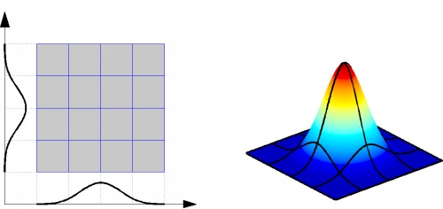
Figure 7: An example of a two-dimensional B-spline basis function, which is a tensor product of two one-dimensional B-splines

One of the most important properties of B-splines is the number of ways in which the basis may be enriched while leaving the underlying geometry and its parameterization unaffected. We consider here two different ways of doing such enrichment: knot insertion and degree elevation. We also want to mention that not only do we have control over the element size and the order of the basis, but we can also control the continuity of the basis as well. We refer to  [19] for the details and  [14] for the applications to IGA.

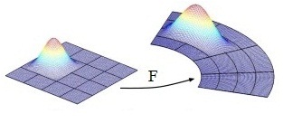
Figure 8: $\mathbf{F}$-mapping and a basis function transformation

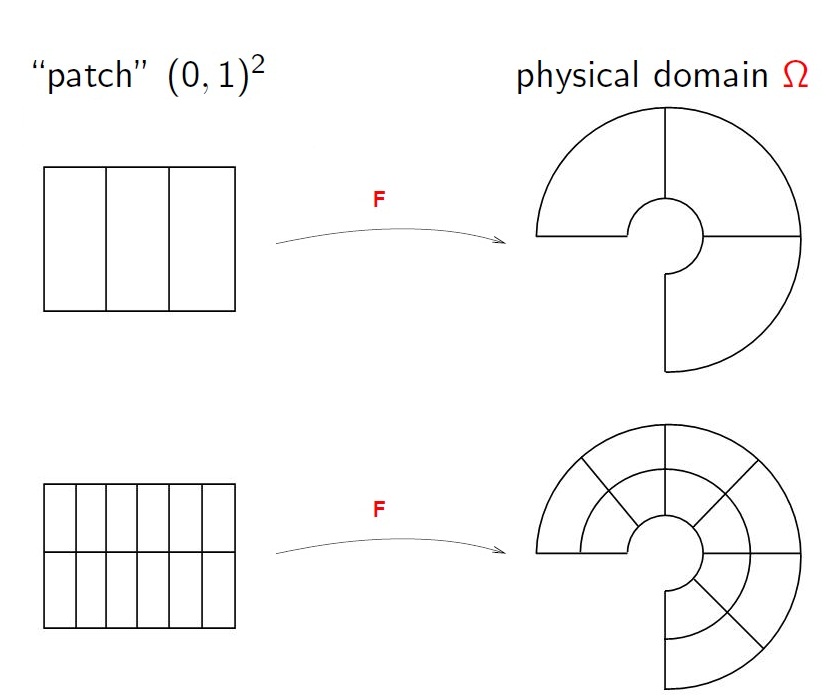
Figure 9: Example of a $\mathbf{F}$-mapping and refinement

3.6 The IsoGeometric Concept

The fundamental idea  behind IGA is that the basis used to exactly model the geometry will also serve as the basis for the solution space of the numerical method. This notion of using the same basis for geometry and analysis is called the Isoparametric concept, and it is quite common in classical finite element analysis. The fundamental difference between the new concept of Isogeometric Analysis and the classic concept of isoparametric finite element analysis is that, in classical FEA, the basis chosen to approximate the unknown solution fields is also used to define the domain . Isogeometric Analysis turns this idea around and selects a basis capable of exactly representing the known geometry and uses it as a basis for the field we wish to approximate. In a sense, we are reversing the isoparametric arrow such that it points from geometry toward the solution space, rather than vice versa.

One of the main concepts of IGA is the geometrical mapping $\mathbf{F}$. It acts on the parametric domain $\widehat{\Omega}$:

$$\mathbf{F}:\widehat{\Omega}\rightarrow\Omega,$$ (3.6.1)

defining the geometrical domain in the physical space. In fact it acts on the basis functions of the parametric space defining both the geometry and the space of approximation functions used for approximating the solutions of PDEs. Figure 8 shows how the shape is constructed and the transformation of a basis function under the $\mathbf{F}$-mapping. In the present work the basis functions will always be NURBS or B-splines.

3.7 Refinement and IGA

One of the important features of IGA is that when refining the parametric domain the geometrical mapping remains the same resulting in preserving the geometry while refining the solution space. Thus, IGA allows us to make local refinements without changing the geometrical shape. An example of a two-dimensional knot-insertion is shown in Figure 9.

One of the drawbacks of IGA is the nonlocal nature of the refinement due to the tensor product structure of the B-splines. The difficulties arise in large scale problems since the number of degrees of freedom grows very fast. Different algorithms, such as T-splines  [8], were introduced into IGA in order to avoid these problems. All of them still makes the refinement non-local since some tensor product structure needs to be preserved.

This led us to think about different methods of local mesh refinement, which would allow us to keep the computational costs low. We propose to use the Domain Decomposition Method. Its main difference from the refinement techniques is that the new refined mesh is an absolutely separated domain and does not match the coarse one, but now we have to perform an iterative procedure in order to obtain the solution.

3.8 The Alternating Schwarz Method

The Alternating Schwarz method belongs to the class of domain decomposition methods for partial differential equations. Domain decomposition methods can be regarded as divide and conquer algorithms. The main idea is the following: given an open domain (we will assume it to possess some additional properties in the sequel, like being smooth and connected) $\Omega$ we partition it into a number of subdomains $\{\Omega_{i}\}_{i=1}^{n}$, satisfying some conditions, and such that $\Omega=\bigcup_{i=1}^{n}\Omega_{i}$. The original problem then can be reformulated as a family of subproblems of reduced size and complexity defined on the subdomains.

One of the major advantages of domain decomposition methods is the natural parallelism in solving the subproblems defined on the subdomains. With the upcoming of parallel computer architectures, domain decomposition methods have become very popular during the last two decades. However the origin goes back to 1870. In  [12], H. A. Schwarz introduced an algorithm to prove the existence of harmonic functions on irregularly shaped domains. Today this algorithm is known as the Alternating Schwarz Method.

In the next section we will define the problem we are going to solve and the main tool we use to solve it: the IGA framework.

4 Notations and the Problem formulation

Given a bounded connected open domain $\Omega$ with Lipshitz continuous $\partial{\Omega}$, let us consider the Poisson equation

$$-\text{{div}}{(k(x)\text{{grad}}{u})}=f \quad\text{in }\Omega,$$ (4.0.1)

$$k(x)\frac{\partial{u}}{\partial{\mathbf{n}}}=h \quad\text{ on }\Gamma_{N},$$ (4.0.2)

$$u=g \quad\text{ on }\Gamma_{D},$$ (4.0.3)

where $\overline{\Gamma_{D}\bigcup\Gamma_{N}}=\partial\Omega$, $\Gamma_{D}\text{ and }\Gamma_{N}$ are disjoint, and $\mathbf{n}$ is the unit outward normal vector on $\partial\Omega$. The functions $f\in\mathcal{H}^{-1}(\Omega),g\in\mathcal{L}^{2}(\Gamma_{D})$ representing the Dirichlet boundary conditions and $h\in\mathcal{L}^{2}(\Gamma_{N})$ representing the Neumann boundary conditions, are all given.

For a sufficiently smooth domain, a unique solution $u$ satisfying $\eqref{eq:poisson}-\eqref{eq:dir_cond}$ is known to exist under some standard conditions.

4.1 Weak form of the problem

The numerical technique we are going to take advantage of begins by defining a weak, or variational, counterpart of $\eqref{eq:poisson}-\eqref{eq:dir_cond}$. To do so, we need to characterize two classes of functions. The first is to be composed of candidate, or trial functions. From the outset, these functions will be required to satisfy the Dirichlet boundary conditions of $\eqref{eq:dir_cond}$.

We may now define the collection of trial functions, denoted by $\mathcal{S}$ as

$$\mathcal{S}=\{u:u\in\mathcal{H}^{1}(\Omega),u|_{\Gamma_{D}}=g\}.$$

The second collection of functions in which we are interested is called the test or weighting functions. This collection is very similar to the trial functions, except that we have the homogeneous counterpart of the Dirichlet boundary conditions:

$$\mathcal{V}=\{w:w\in\mathcal{H}^{1}(\Omega),w|_{\Gamma_{D}}=0\},$$ (4.1.1)

which is a Hilbert space with respect to the associated energy norm $||u||=a(u,u)^{1/2}$, that follows from the coercivity of the bilinear form $a(\cdot,\cdot)$, as shown below.

We may now obtain a variational statement of our boundary value problem by multiplying the equation $\eqref{eq:poisson}$ by an arbitrary test function $w\in\mathcal{V}$ and integrating by parts, incorporating $\eqref{eq:neum_cond}$ as needed.

Given $f,g$ and $h$ find $u\in\mathcal{S}$ such that for all $w\in\mathcal{V}$

$$\int_{\Omega}k(x)\textbf{grad}w\cdot\textbf{grad}u\textbf{d}\Omega=\int_{\Omega}wf\textbf{d}\Omega+\int_{\Gamma_{N}}wh\textbf{d}\Gamma.$$ (4.1.2)

Define a bilinear form $a(\cdot,\cdot):\mathcal{H}^{1}(\Omega)\times\mathcal{H}^{1}(\Omega)\rightarrow\mathbb{R}$ and a functional $L:\mathcal{H}^{1}(\Omega)\rightarrow\mathbb{R}$ as:

$$a(w,u)=\int_{\Omega}k(x)\textbf{grad}w\cdot\textbf{grad}u\textbf{d}\Omega,$$ (4.1.3)

and

$$L(w)=\int_{\Omega}wf\textbf{d}\Omega+\int_{\Gamma_{N}}wh\textbf{d}\Gamma.$$ (4.1.4)

Now the weak form reads as:

$$a(w,u)=L(w),$$ (4.1.5)

We shall note here, that the bilinear functional $a(\cdot,\cdot)$ is symmetric and positive definite for any $k(x)>0$ when considered over the space $\mathcal{V}$. Indeed, as shown below it is coercive, which results in the symmetry and positive definiteness of the stiffness matrix we are going to define below . One will find in (CIARLET) that the above problem  4.1.5 has a unique solution in $\mathcal{H}^{1}(\Omega)$.

4.2 Galerkin’s Method

In Galerkin’s method we define finite-dimensional approximations of the spaces $\mathcal{S}$ and $\mathcal{V}$, denoted $\mathcal{S}_{h}$ and $\mathcal{V}_{h}$ such that $\mathcal{S}_{h}\subset\mathcal{S},$ $\mathcal{V}_{h}\subset\mathcal{V}$. These subspaces will be associated with subsets of the space spanned by the isogeometric basis.

As we have just mentioned we can further characterize $\mathcal{S}_{h}$ by recognizing that if we have a given function $g_{h}\in\mathcal{S}_{h}$ such that $g_{h}|_{\Gamma_{D}}=g$, then for every $u_{h}\in\mathcal{S}_{h}$ there exists a unique $v_{h}\in\mathcal{V}_{h}$ such that

$$u_{h}=v_{h}+g_{h}.$$

This clearly will not be possible for an arbitrary function $g$. The problem of approximation of the function $g$ by a function $g_{h}\in\mathcal{S}_{h}$ will be treated in detail below. So let us assume at present that such a function $g_{h}$ exists.

As in  [14] we can write the Galerkin’s form of the problem as: given $g_{h}$ and $h$, find $u_{h}=v_{h}+g_{h}$, where $v_{h}\in\mathcal{V}_{h}$, such that for all $w_{h}\in\mathcal{V}_{h}$

$$a(w_{h},u_{h})=L(w_{h}),$$ (4.2.1)

or

$$a(w_{h},v_{h})=L(w_{h})-a(w_{h},g_{h}).$$ (4.2.2)

We will use this form for the variational formulation for the Schwarz Method.

In general the weighting space $\mathcal{V}_{h}$ of test functions may be different than the space $\widetilde{\mathcal{V}}_{h}$ of trial functions $v_{h}$, that is $v_{h}\in\mathcal{V}_{h}$ but $w_{h}\in\widetilde{\mathcal{V}}_{h}\neq\mathcal{V}_{h}$, but in the following we will assume they are the same.

5 General IGA

The goal of IGA, as it is also for FEM, is the numerical approximation of the solution of partial differential equations (PDEs) [4]. In both approaches the PDEs are numerically solved using the Galerkin procedure: the equations are written in there equivalent variational formulations, and a solution is sought in a finite dimensional space with good approximation properties. The main difference between the two methodologies is that in FEM the basis functions and the computational geometry (i.e., the mesh) are defined element by element, using piecewise polynomial approximations, whereas in IGA the computational geometry and the space are defined exactly from the (input data) information and the basis functions (e.g., NURBS, T-splines or generalized B-splines) given by CAD.

Another important difference is that the unknowns to be computed, coefficients that define the solution as a linear combination of the basis functions (degrees of freedom), are not nodal values, but “control values” .

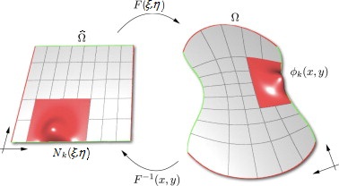
Figure 10: Example of a $\mathbf{F}$-mapping and the basis function transformation

Let us consider a two-dimensional case where we assume that the physical domain $\Omega\subset\mathbb{R}^{2}$ is open, bounded and piecewise smooth. We also assume that such a domain can be exactly described through a parametrization of the form

$$\mathbf{F}:\widehat{\Omega}\rightarrow\Omega,$$ (5.0.1)

where $\widehat{\Omega}$ is some parametric domain (e.g., the unit square), and the value of the parameterization can be computed via the isogeometric mapping $\mathbf{F}$, which is assumed to be smooth with piecewise smooth inverse, see Figure 10.

We now construct the finite-dimensional spaces $\mathcal{S}_{h}$ and $\mathcal{V}_{h}$ as spans over their basis functions:

$$\mathcal{S}_{h}:=\langle\phi_{1},\phi_{2},...,\phi_{N_{h}},\phi_{N_{h}+1},...,\phi_{N_{h}+N_{h}^{b}}\rangle\subset\mathcal{S},$$

and

$$\mathcal{V}_{h}:=\langle\phi_{1},\phi_{2},...,\phi_{N_{h}}\rangle\subset\mathcal{V},$$

where we first number all the basis function which vanish on the boundary $\Gamma_{D}$: $\phi_{1},\phi_{2},...,\phi_{N_{h}}$, and then the other basis functions $\phi_{N_{h}+1},...,\phi_{N_{h}+N_{h}^{b}}$, which do not vanish on this boundary.

The IGA prescribes us the way of building the basis functions for the spaces $\mathcal{S}_{h}$ and $\mathcal{V}_{h}$. Let $\{\widehat{\phi}_{j}\}_{j\in\mathcal{I}\cup\mathcal{B}}$ be a basis for $\widehat{\mathcal{S}}_{h}$, with $\mathcal{I}\cup\mathcal{B}$ a proper set of indices; we partition the indices in the same way as before: $\mathcal{I}$ corresponds to the basis functions that vanish on the boundary $\widehat{\Gamma}_{D}$ and $\mathcal{B}$ corresponds to those which do not vanish on $\widehat{\Gamma}_{D}$. With the assumption made on $\mathbf{F}$, the set $\{\widehat{\phi}_{j}\circ\mathbf{F}^{-1}\}_{j\in\mathcal{I}\cup\mathcal{B}}\equiv\{\phi_{j}\}_{j\in\mathcal{I}\cup\mathcal{B}}$ is a basis for $\mathcal{S}_{h}$ and $\{\widehat{\phi}_{j}\circ\mathbf{F}^{-1}\}_{j\in\mathcal{I}}\equiv\{\phi_{j}\}_{j\in\mathcal{I}}$ is a basis for $\mathcal{V}_{h}$.

In IGA, as introduced in [14], the spaces $\mathcal{S}_{h}$ and $\mathcal{V}_{h}$ are formed by transformation of B-spline functions. We define these space in the following general way:

$$\mathcal{S}_{h}:=\{u_{h}\in\mathcal{S}:\widehat{u}_{h}=u_{h}\circ\mathbf{F}\in\widehat{\mathcal{S}}_{h}\}\equiv\{u_{h}\in\mathcal{S}:u_{h}=\widehat{u}_{h}\circ\mathbf{F}^{-1},\widehat{u}_{h}\in\widehat{\mathcal{S}}_{h}\},$$ (5.0.2)

$$\mathcal{V}_{h}:=\{v_{h}\in\mathcal{V}:\widehat{v}_{h}=v_{h}\circ\mathbf{F}\in\widehat{\mathcal{V}}_{h}\}\equiv\{v_{h}\in\mathcal{V}:v_{h}=\widehat{v}_{h}\circ\mathbf{F}^{-1},\widehat{v}_{h}\in\widehat{\mathcal{V}}_{h}\},$$ (5.0.3)

where $\iota$ is a proper pull-back, defined from the parametrization $\eqref{eq:parameterization}$, and $\widehat{\mathcal{S}}_{h}$ and $\widehat{\mathcal{V}}_{h}$ are finite spaces generated by the basis functions defined in the parametric domain $\widehat{\Omega}$.

Hence, the discrete solution of the problem can be written as

$$u_{h}=\sum_{j\in\mathcal{I}\cup\mathcal{B}}\alpha_{j}\phi_{j}=\sum_{j\in\mathcal{I}\cup\mathcal{B}}\alpha_{j}\widehat{\phi}_{j}\circ\mathbf{F}^{-1}.$$ (5.0.4)

We assume that for the function $g$ representing the Dirichlet boundary conditions, there exists a function $g_{h}\in\mathcal{S}_{h}$ such that $g_{h}|_{\Gamma_{D}}=g$, meaning that there exist $\{\gamma_{j}\}_{j\in\mathcal{B}}$ such that $g=\sum_{j\in\mathcal{B}}\gamma_{j}\phi_{j}$. The more general case of $g\in\mathcal{S}$ will be treated below.

The solution now read as

$$u_{h}=\sum_{j\in\mathcal{B}}\gamma_{j}\phi_{j}+\sum_{j\in\mathcal{I}}\alpha_{j}\phi_{j}.$$

Thus, instead of considering the function $u_{h}\in\mathcal{S}_{h}$ we can treat without loss of generality the function $u_{h}-\sum_{j\in\mathcal{B}}\gamma_{j}\phi_{j}\in\mathcal{V}_{h}$, reducing the problem to the homogeneous Dirichlet boundary conditions case. So we can write

$$u_{h}=\sum_{j\in\mathcal{I}}\alpha_{j}\phi_{j}.$$

Substituting this expression into $\eqref{eq:discr_var_form}$, and testing against every test function $\phi_{i}\in\mathcal{V}_{h}$, we obtain a linear system of equations where the coefficients $\alpha_{j}$ are the unknowns, and the entries of the matrix and the right-hand side are $a(\phi_{i},\phi_{j})$ and $L(\phi_{i})$, respectively.

$$a({\sum_{j\in\mathcal{I}}\alpha_{j}\phi_{j}},\phi_{i})=L(\phi_{i}),\forall i\in\mathcal{I}$$ (5.0.5)

These terms have to be computed using suitable quadrature rules for numerical integration [14].

6 Model Problem: Poisson Equation with homogeneous Dirichlet BC

We now specialize the general framework of the previous section to the particular case of the Poisson’s problem $\eqref{eq:poisson}-\eqref{eq:dir_cond}$, defined in a physical domain $\Omega$ described and discretized with B-Splines. This constitutes the model problem on which we show in detail the IGA method.

Let us assume that the computational domain is constructed as a singleB-Spline patch, such that the parameterization $\mathbf{F}$ is given as above, see Figure 10. The assumptions on $\mathbf{F}$ of the previous section are here supposed to be valid. For the sake of simplicity, homogeneous Dirichlet boundary conditions are assumed.

The linear equations from 5.0.5 can be rewriten as:

$$\sum_{j=1}^{N_{h}}A_{ij}\alpha_{j}=f_{i}+h_{i}\text{ for }i=1,\dots,N_{h},$$ (6.0.1)

where

$$A_{ij}=\int_{\Omega}k(x)\text{{grad}}\phi_{j}\text{{grad}}\phi_{i}\textbf{d}x\text{ for }i,j=1,\dots,N_{h},$$ (6.0.2)

$$f_{i}=\int_{\Omega}f\phi_{i}\textbf{d}x\text{ for }i=1,\dots,N_{h},$$ (6.0.3)

$$h_{i}=\int_{\Gamma_{N}}h\phi_{i}\textbf{d}\Gamma\text{ for }i=1,\dots,N_{h}.$$ (6.0.4)

Here $A_{ij}$ are the coefficients of the stiffness matrix, and $f_{i}$ and $g_{i}$ are the coefficients of the right-hand side contributions from the source and the boundary terms, respectively. All the coefficients are given by the values of the integrals in $\eqref{eq:source}$, that are numerically approximated by a suitable quadrature rule [14].

In order to describe this rule, let us introduce $\widehat{\mathcal{K}}_{h}:=\{\widehat{K}_{k}\}_{k=1}^{N_{e}}$, a partition of the parametric domain $\widehat{\Omega}$ into $N_{e}$ non-overlapping subregions, that henceforth we will refer to as $elements$. The assumptions on the parameterization $\mathbf{F}$ ensure that the physical domain $\Omega$ can be partitioned as

$$\overline{\Omega}=\bigcup_{k=1}^{N_{e}}\mathbf{F}(\widehat{K}_{k}),$$

and the corresponding elements $K_{k}:=\mathbf{F}(\widehat{K}_{k})$ are also non-overlapping. We will denote this partition by $\mathcal{K}_{h}:=\{K_{k}\}_{k=1}^{N_{e}}$.

For the sake of generality, let us assume that a quadrature rule is defined on every element $\widehat{\mathcal{K}}_{k}$. Each of these quadrature rules is determined by a set of $n_{k}\textit{ quadrature nodes}$:

$$\{\widehat{x}_{l,k}\}\subset\widehat{K}_{k},l=1,...,n_{k}$$

and by their corresponding weights

$$\{w_{l,k}\}\subset\mathbb{R},l=1,...,n_{k}.$$

In this work we use Gaussian quadrature rules as described in  [14].

After introducing a change of variable, the integral of a generic function $\phi\in\mathcal{L}^{1}(K_{k})$ is approximated as follows

$$\int_{K_{k}}\phi dx=\int_{\widehat{K}_{k}}\phi(\mathbf{F}(\widehat{x}))|\det(D\mathbf{F}(\widehat{x}))|d\widehat{x}\simeq\sum_{i=1}^{n_{k}}w_{l,k}\phi(x_{l,k})|\det(D\mathbf{F}(\widehat{x}_{l,k}))|,$$ (6.0.5)

where $x_{l,k}:=\mathbf{F}(\widehat{x}_{l,k})$ are the images of the quadrature nodes in the physical domain, and $D\mathbf{F}$ is the Jacobian matrix of the parameterization $\mathbf{F}$.

Using the quadrature rule, the coefficients of the stiffness matrix are numerically computed as

$$A_{ij}\simeq\sum_{k=1}^{N_{e}}\sum_{l=1}^{n_{k}}k(x_{l,k})w_{l,k}\text{{grad}}\phi_{j}(x_{l,k})\text{{grad}}\phi_{i}(x_{l,k})|\det(D\mathbf{F}(\widehat{x}_{l,k}))|,$$ (6.0.6)

while the coefficients $f_{i}$ of the right-hand side are approximated as

$$f_{i}\simeq\sum_{k=1}^{N_{e}}\sum_{l=1}^{n_{k}}f(x_{l,k})w_{l,k}\phi_{i}(x_{l,k})|\det(D\mathbf{F}(\widehat{x}_{l,k}))|.$$ (6.0.7)

7 Dirichlet boundary conditions

The imposition of homogeneous boundary conditions in IGA is straightforward. In fact, homogeneous Neumann conditions are satisfied naturally because they are included in the weak formulation itself. On the contrary, as far as non-homogeneous Dirichlet boundary conditions are concerned, a suitable transformation has to be applied to reduce the problem to the case of homogeneous boundary conditions since there is no place in the Galerkin formulation of the problem where the Dirichlet boundary conditions can be imposed. For this reason we must build them directly into the solution space.

In FEM the imposition of Dirichlet boundary conditions can be performed easily since the basis functions are interpolatory and local. On the contrary, in IGA the treatment of the Dirichlet boundary conditions is a much more involved problem. The basis functions (B-splines or NURBS) are not local, nor interpolatory.

In section 5 we assumed that there exists a function $g_{h}\in\mathcal{S}_{h}$ such that $g_{h}|_{\Gamma_{D}}=g$, and refered to this function as a lifting. In practice, this will frequently be the case, but there will also be instances in which a lifting is only an approximation of $g$.

The standard approach consists in constructing a function $R_{g}$ as suitable extension of $g$ such that

$$R_{g}\in\mathcal{H}^{1}(\Omega),$$

$$R_{g}=g\text{ on }\Gamma_{D},$$

and consider the problem $\eqref{eq:gen_weak},\eqref{eq:var_form}$ for the difference $u-R_{g_{D}}$, see  [6] for details. To construct an approximation of $R_{g_{D}}$ it is necessary to have an approximation of the boundary data function $g$. A possible strategy consists in obtaining an approximation $g_{h}$ of $g$ in the space

$$\mathcal{S}_{h}\backslash\mathcal{V}_{h}:=\langle\phi_{N_{h}+1},\dots,\phi_{N_{h}+N_{h}^{b}}\rangle.$$

as combination of the $N_{h}^{b}$-basis functions of $\mathcal{S}_{h}$ which do not vanish on $\Gamma_{D}$, that is

$$g_{h}(\textbf{x}):=\sum_{N_{h}+1}^{N_{h}+N_{h}^{b}}q_{i}\phi_{i}|_{\Gamma_{D}}(\textbf{x}),\text{ }\forall\textbf{x}\in\Gamma_{D}.$$ (7.0.1)

Then, an approximation of $R_{g}$ in $\mathcal{S}_{h}$, can be constructed as:

$$R_{g_{h}}(\textbf{x}):=\sum_{N_{h}+1}^{N_{h}+N_{h}^{b}}q_{i}\phi_{i}(\textbf{x}),\text{ }\forall\textbf{x}\in\Omega_{h}.$$ (7.0.2)

The control variables $q_{i}$ in $\eqref{eq:bound1}$ have to be computed according to the approximation method used .

The easiest way is to apply these conditions directly to the control variables, as

$$g_{h}(\textbf{x}):=\sum_{N_{h}+1}^{N_{h}+N_{h}^{b}}g(\overline{\mathbf{\xi}}_{i})\phi_{i}|_{\Gamma_{D}}(\textbf{x}),\text{ }\forall\textbf{x}\in\Gamma_{D};$$

for proper values $\overline{\mathbf{\xi}}_{i},\text{ }i=N_{h}+1,\dots,N_{h}+N_{h}^{b}$. Such a strategy may result in a lack of accuracy in case of inhomogeneous conditions and a poor accuracy of the approximated solution, even if spaces $\mathcal{V}_{h}$ with high approximation power are used.

A standard approach consists in imposing Dirichlet boundary conditions by interpolation of the boundary data $g$. Another way of imposing Dirichlet boundary conditions is to use least-squares approximation of the given function $g$ by a B-spline. We will review both methods.

7.1 Least-squares approximation of the Dirichlet boundary conditions

The least-squares approximation of the function $g$ consists in solving an optimization problem. More exactly, we need to find such coefficients $\{\widetilde{q}_{i}\}_{i=N_{h}+1}^{N_{h}+N_{h}^{b}}$ which would minimize the following integral:

$$\min_{\{q_{i}\}_{i=N_{h}+1}^{N_{h}+N_{h}^{b}}}\int_{\Gamma_{D}}(g(\textbf{x})-\sum_{N_{h}+1}^{N_{h}+N_{h}^{b}}q_{i}\phi_{i}(\textbf{x}))^{2}\textbf{d}\Gamma.$$ (7.1.1)

We perform the following transformations of the integral in $\eqref{eq:ls}$:

$$\begin{split}&\int_{\Gamma_{D}}\left(g(\textbf{x})-\sum_{i=N_{h}+1}^{N_{h}+N_{h}^{b}}q_{i}\phi_{i}(\textbf{x})\right)^{2}\textbf{d}\Gamma=\\ &\int_{\Gamma_{D}}(g(\textbf{x}))^{2}\textbf{d}\Gamma-2\int g(\textbf{x})\sum_{N_{h}+1}^{N_{h}+N_{h}^{b}}q_{i}\phi_{i}(\textbf{x})\textbf{d}\Gamma+\int\sum_{i,j=N_{h}+1}^{N_{h}+N_{h}^{b}}q_{i}q_{j}\phi_{i}(\textbf{x})\phi_{j}(\textbf{x})\textbf{d}\Gamma.\end{split}$$ (7.1.2)

Let us rewrite this equation in the following form:

$$\int_{\Gamma_{D}}\left(g(\textbf{x})-\sum_{i=N_{h}+1}^{N_{h}+N_{h}^{b}}q_{i}\phi_{i}(\textbf{x})\right)^{2}\textbf{d}\Gamma=\int_{\Gamma_{D}}(g(\textbf{x}))^{2}\textbf{d}\Gamma-2\textbf{q}^{T}\textbf{g}+\textbf{q}^{T}\textbf{M}\textbf{q},$$ (7.1.3)

where

$$\textbf{q}=(q_{N_{h}+1}\dots q_{N_{h}+N_{h}^{b}}),$$ (7.1.4)

$$\textbf{g}=\begin{pmatrix}\int g(\textbf{x})\phi_{N_{h}+1}(\textbf{x})\textbf{d}\Gamma\\ \vdots\\ \int g(\textbf{x})\phi_{N_{h}+N_{h}^{b}}(\textbf{x})\textbf{d}\Gamma\end{pmatrix},$$ (7.1.5)

and $\textbf{M}=\{\int\phi_{i}(\textbf{x})\phi_{j}(\textbf{x})\textbf{d}\Gamma\}_{i,j=N_{h}+1}^{N_{h}+N_{h}^{b}}$ is the mass matrix.

In order to minimize our target function we just differentiate it once with respect to the coefficients $q_{i}$ to get the closed form solution:

$$\textbf{q}=\textbf{M}\backslash\textbf{g}.$$ (7.1.6)

The matrix M being invertible since it is the Gram matrix of the basis functions of the boundary $\partial\Omega$ which is a union of NURBS or B-spline patches in the standard $\mathcal{L}^{2}$ inner product.

We consider the boundary of the physical domain $\Gamma$ which is an image of the boundary $\widehat{\Gamma}$ under the isogeometric mapping $\mathbf{F}$ and is itself a union of NURBS or B-spline patches with dimensions one less than the dimension of the original patch $\Omega$. So we may decompose the boundary $\Gamma=\cup_{i}\gamma_{i}$ into a union of NURBS patches and consider the minimization problem of approximating the boundary function on each of them.

After we have computed the Dirichlet degrees of freedom $\tilde{q}_{i}$, we can construct the desired function

$$R_{g_{h}}(\textbf{x}):=\sum_{N_{h}+1}^{N_{h}+N_{h}^{b}}\tilde{q}_{i}\phi_{i}(\textbf{x}),\text{ }\forall\textbf{x}\in\Omega_{h}.$$ (7.1.7)

We now solve the homogenous problem in the variational form:

$$a(w_{h},u_{h}-R_{g_{h}})=L(w_{h}),\forall w_{h}\in V_{h},$$ (7.1.8)

where we have only the first $N_{h}$ degrees of freedom to be found from this linear system.

7.2 Quasi-interpolation of the Dirichlet boundary conditions

Here we consider the point-wise approximation: we are looking for a B-spline function (on the given part of the boundary) which coincides with $g$ at a number of points in the spirit of collocation.

Consider a two-dimensional domain. Assume that we deal with a part of boundary $\gamma$ that corresponds to one side of the parametric domain square and there are $n$ degrees of freedom corresponding to this part of boundary. We want to take some $n$ points on the curve $\gamma$ and make the B-spline function we are looking for coincide with $g$ at these point. This gives as a square system of linear equations:

$$\sum_{j=1}^{n}q_{j}\phi_{j}(x_{i},y_{i})=g(x_{i},y_{i}),i=1\dots n.$$ (7.2.1)

In order to solve this system we must require its matrix to be non-singular, and this obviously depends on the choice of the points ${(x_{i},y_{i})}_{i=1}^{n}$. In our work we chose the $n$ points to be the images of the centers of the $n$ knot-spans of the parametric domain. It may be easily shown that the matrix we obtain in such a case is nonsingular. Indeed, we know that the monomials form a totally positive basis on the interval $[0,1]$ and B-splines are obtained from them by the transformations saving the totally positivity properties  [5], consequently the B-spline basis we have is also totally positive and the matrix we get is nonsingular.

Thus, the system now looks like:

$$\sum_{j=1}^{n}q_{j}\widehat{\phi_{j}}(\xi_{i},\eta_{i})=g(\mathbf{F}(\xi_{i},\eta_{i})),i=1\dots n,$$ (7.2.2)

for the specific $\{(\xi_{i},\eta_{i})\}_{i=1}^{n}$ we choose.

One of the questions we are interested in is how to choose these points optimally for the B-spline and NURBS geometry.

Applying the same algorithm to all the sides of the domain where the Dirichlet boundary conditions are imposed we may compute all the Dirichlet degrees of freedom.

There are also other approaches if imposing the Dirichlet boundary conditions such as local least-squares, see  [11] or Nitsche’s method [2] .

8 Neumann boundary conditions

Neumann boundary conditions of the form $\eqref{eq:neum_cond}$ are frequently referred to as natural boundary conditions. This is because of the way they automatically arise in the variational statement of a problem. Let us assume for the moment without loss of generality that $k(x)=1$ and that the Dirichlet conditions have already been imposed. Multiplying by a test function and integrating leads us to

$$\begin{split}&0=\int_{\Omega}w(\triangle u+f)d\Omega\\ &=-\int_{\Omega}\nabla w\nabla ud\Omega+\int_{\Gamma}w\nabla u\cdot\mathbf{n}d\Gamma+\int_{\Omega}wfd\Omega\\ &=-\int_{\Omega}\nabla w\nabla ud\Omega+\int_{\Gamma_{N}}w\nabla u\cdot\mathbf{n}d\Gamma+\int_{\Omega}wfd\Omega,\end{split}$$ (8.0.1)

where in the third line we have used the fact that the weighting space is defined such that $w|_{\Gamma_{D}}=0$.

The integration by parts has naturally introduced a boundary integral over $\Gamma_{N}$ that refers explicitly to the condition that we would like to impose. Using the condition $\eqref{eq:neum_cond}$ we simply replace $\nabla u\cdot\mathbf{n}$ with the value we are imposing, $h$, resulting in

$$-\int_{\Omega}\nabla w\nabla ud\Omega+\int_{\Gamma}whd\Gamma+\int_{\Omega}wfd\Omega=0.$$ (8.0.2)

Now that we have formulated a discretized analog of the original problem in the next chapter we are going to consider a variant of Schwarz Domain Decomposition Method to solve it.

9 Schwarz Additive Domain Decomposition Method

9.1 Notations

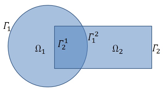
Figure 11: Domain Decomposition

Consider the two-dimensional domain $\Omega$ as shown in the Figure 11, which can be represented as a union of two overlapping subdomains $\Omega=\Omega_{1}\cup\Omega_{2}$. In this work we consider only domains which satisfy some reasonable conditions: they are connected and piecewise smooth boundary. We want to solve the Poisson problem $\eqref{eq:poisson}-\eqref{eq:dir_cond}$ on this complex domain. We denote by $\Gamma_{i},i=1,2$ the part of the boundary of $\Omega_{i}$ which belongs to the boundary $\partial\Omega$ of the whole domain and by $\Gamma_{i}^{j},i,j=1,2,i\neq j$ the boundary of $\Omega_{i}$, which belongs to the second subdomain: $\Gamma_{i}^{j}=\partial\Omega_{i}\cap\Omega_{j}$. The earliest known domain decomposition method is the Alternating Schwarz Method (ASM) dating back to 1870 [12]. The original alternating Schwarz method is a sequential method that successively solves the following problems: given the Dirichlet boundary conditions function $g$ on $\Gamma$ and starting with the initial guess $u_{2}^{0}=0$ (in particular $u_{2}^{0}|_{\Gamma_{1}^{2}}=0$), iteratively obtain solutions $u_{1}^{n}(x,y)$ and $u_{2}^{n}(x,y)$ on $\Omega_{1}$ and $\Omega_{2}$ respectively $(n\in\mathbb{N})$ [17],

$$\triangle u_{1}^{n}=f \quad\text{ in }\Omega_{1},$$ (9.1.1)

$$u_{1}^{n}=g_{1}^{n} \quad\text{ on }\Gamma_{1D},$$ (9.1.2)

where $g_{1}^{n}|_{\Gamma_{1}^{2}}=u_{2}^{n-1}|_{\Gamma_{1}^{2}},g_{1}^{n}|_{\Gamma_{1}}=g|_{\Gamma_{1}}$ and

$$\triangle u_{2}^{n}=f \quad\text{ in }\Omega_{2},$$ (9.1.3)

$$u_{2}^{n}=g_{2}^{n} \quad\text{ on }\Gamma_{2D},$$ (9.1.4)

where $g_{2}^{n}|_{\Gamma_{2}^{1}}=u_{1}^{n}|_{\Gamma_{2}^{1}},g_{2}^{n}|_{\Gamma_{2}}=g|_{\Gamma_{2}}$. It is important to notice that the solution of the first problem is required before the second problem can be solved. The part of the boundary conditions of the second problem, $g_{2}^{n}=u_{1}^{n}|_{\Gamma_{2}^{1}}$, is the current solution of the first problem on the interface. It is not difficult to see that in this simple case of two subdomains it is an analog of a block Gauss-Seidel method and the two problems cannot be solved in parallel. For a straight forward parallelization of the algorithm an analog of the block Jacobi method is applied giving us the Schwarz Additive method:

$$\triangle u_{1}^{n}=f \quad\text{ in }\Omega_{1},$$ (9.1.5)

$$u_{1}^{n}=g_{1}^{n} \quad\text{ on }\Gamma_{1D},$$ (9.1.6)

where $g_{1}^{n}|_{\Gamma_{1}^{2}}=u_{2}^{n-1}|_{\Gamma_{1}^{2}},g_{1}^{n}|_{\Gamma_{1}}=g|_{\Gamma_{1}}$, and

$$\triangle u_{2}^{n}=f \quad\text{ in }\Omega_{2},$$ (9.1.7)

$$u_{2}^{n}=g_{2}^{n} \quad\text{ on }\Gamma_{2D},$$ (9.1.8)

where $g_{2}^{n}|_{\Gamma_{2}^{1}}=u_{1}^{n-1}|_{\Gamma_{2}^{1}},g_{2}^{n}|_{\Gamma_{2}}=g|_{\Gamma_{2}}$.

The iterative procedure starts given two initial guesses $u_{1}^{0}$ and $u_{2}^{0}$ on each subdomain. The boundary condition of one of the subproblems, $g_{j}^{n}=u_{i}^{n-1}|_{\Gamma_{j}^{i}},i,j=1,2,i\neq j$ is now the solution of the previous iterate on the interface, hence the subproblems can be solved independently. In the general case of many subdomains a great deal of parallelism can be introduced, using a method called multi-coloring. This is a graph theory technique that identifies each subdomain with a color such that disjoint subdomains have the same color; usually only a small number of colors is needed. Thus, the subproblems defined on subdomains of the same color can be solved independently in parallel and only the number of distinct colors different threads is needed to perform the computations. We are using such techniques below when considering 3-dimensional multi-patched domains.

For the ASDDM as presented here, one can see that there is no notion of a global approximate solution. One can consider defining the global solution by choosing the subdomain iterative solution on each subdomain and any weighted average within the overlap:

$$u^{n}=\chi_{1}v^{n}+\chi_{2}w^{n},$$

where $\chi_{1}=1$ on $\Omega_{1}\backslash(\Omega_{1}\cap\Omega_{2})$, $\chi_{2}=1$ on $\Omega_{2}\backslash(\Omega_{1}\cap\Omega_{2})$ and $\chi_{1}+\chi_{2}=1$ on $\Omega_{1}\cap\Omega_{2}$. This approach extends easily to a case of multi-patched domain decomposition.

9.2 Convergence conditions

The iterations are performed until certain convergence conditions are met. Throughout this work we consider the $\mathcal{L}^{2}$ errors as the termination condition. In the model problems when the exact solution is known the errors are calculated as a $\mathcal{L}^{2}$ norms between the approximate solution and the exact one.

Assume the exact solution $u_{ex}\in\mathcal{H}^{1}$ is given. Then the error is calculated as

$$\begin{split}&||u_{h}-u_{ex}||_{2}^{2}=\int_{\Omega}(u_{h}-u_{ex})^{2}dx=\int_{\Omega}\left(\sum_{j\in\mathcal{J}_{i}\cup\mathcal{J}_{b}}\alpha_{j}\phi_{j}-u_{ex}\right)^{2}dx=\\ &\sum_{k}\int_{K_{k}}\left(\sum_{j\in\mathcal{J}_{i}\cup\mathcal{J}_{b}}\alpha_{j}\phi_{j}-u_{ex}\right)^{2}dx.\end{split}$$ (9.2.1)

We sum up the integrals on the elements and perform numerical integration element-wise. Assume that an integration rule is given by the mesh of points $\{\widehat{x}_{l,k}\}_{l,k}$ and weights $\{w_{l,k}\}_{l,k}$. For each element $K_{k}$ we obtain:

$$\begin{split}&\int_{K_{k}}\left(\sum_{j\in\mathcal{J}_{i}\cup\mathcal{J}_{b}}\alpha_{j}\phi_{j}-u_{ex}\right)^{2}dx\\ &=\int_{\widehat{K}_{k}}\left(\sum_{j\in\mathcal{J}_{i}\cup\mathcal{J}_{b}}\alpha_{j}\phi_{j}(\mathbf{F}(\widehat{x})))-u_{ex}(\mathbf{F}(\widehat{x})))\right)^{2}\det(D\mathbf{F}(\widehat{x}))|d\widehat{x}\\ &\simeq\sum_{i=1}^{n_{k}}w_{l,k}\left(\sum_{j\in\mathcal{J}_{i}\cup\mathcal{J}_{b}}\alpha_{j}\phi_{j}(\mathbf{F}(\widehat{x}_{l,k})))-u_{ex}(\mathbf{F}(\widehat{x}_{l,k})))\right)^{2}|\det(D\mathbf{F}(\widehat{x}_{l,k}))|.\end{split}$$ (9.2.2)

This numerical integration formula was implemented in the code we used. An analogous formula for the $\mathcal{H}^{1}$ errors can also be developed.

10 Weak form of ASDDM

We may now obtain a variational form of the ASDDM method for the equations $\eqref{eq:SADD3-1}-\eqref{eq:SADD4-3}$.

We are looking for two functions $u_{i}\in\mathcal{H}^{1}(\Omega_{i}),i=1,2$ such that their weighted sum $u=\chi_{1}u_{1}+\chi_{2}u_{2}$ satisfies the Poisson equation $\eqref{eq:poisson}-\eqref{eq:dir_cond}$ or its weak form 4.1.5.

This weak form of the iterative ASDDM now reads as:

Algorithm 1 ASDDM Weak form

  Given $u_{i}^{0}\in\mathcal{H}^{1}(\Omega_{i}),i=1,2$, such that $u_{i}^{0}|_{\Gamma_{i}}=g|_{\Gamma_{i}},i=1,2$,

  Define convergence level $\varepsilon$

  while  $Error\geq\varepsilon$  do

     Find $u_{i}^{n}\in\mathcal{H}^{1}(\Omega_{i}):$ such that $u_{i}^{n}|_{\Gamma_{i}^{j}}=u_{j}^{n-1}|_{\Gamma_{i}^{j}}\text{ and }u_{i}^{n}|_{\Gamma_{i}}=g|_{\Gamma_{i}}$

     

$$\int_{\Omega_{i}}\textbf{grad}v\cdot\textbf{grad}u_{i}^{n}\textbf{d}\Omega=\int_{\Omega_{i}}vf\textbf{d}\Omega+\int_{\Gamma_{iN}}vh\textbf{d}\Gamma$$

      for any $v\in\mathcal{H}_{0}^{1}(\Omega_{i}),i,j=1,2,i\neq j$.

  end while

11 Operator form of the algorithm

In order to proceed to the finite dimensional space computations from this continuous settings we need to introduce a few operators. Assume that the solution $u_{i}^{n}$ on the $\Omega_{i}$ domain is sought in the finite dimensional space $\mathcal{S}_{i}$. Given a function $u_{j}^{n}\in\mathcal{H}^{1}(\Omega_{j})$ our aim is to impose the Dirichlet boundary conditions on the $\Omega_{i}$ domain, which requires us to find a function $g_{i}\in\mathcal{S}_{i}$ which will be close in some specific sense to the function $u_{j}$ on the interface boundary $\Gamma_{i}^{j}$.

We proceed as following: first we need to project the function $u_{j}^{n}$ onto the boundary $\Gamma_{i}^{j}$ to get a function $\widetilde{g}\in\mathcal{L}^{2}(\Gamma_{i}^{j})$ representing the Dirichlet boundary conditions on this part of the boundary. We refer to this operator as a trace operator.

The next steps depend on whether the space $\mathcal{S}_{i}$ contains a function which is an extension of $\widetilde{g}$ or not. If it does we just take any extension of $\widetilde{g}$ satisfying the Dirichlet boundary conditions on the parts of the boundary $\Gamma_{i}$ and continue the solution process as in the regular IGA case, see section (3.2.1). We refer to the operator building the extension as extension operator. If $\mathcal{S}_{i}$ does not contain an extension of $\widetilde{g}$ we need to find a function in $\mathcal{S}_{i}$ that would approximate the $\widetilde{g}$ on the boundary $\Gamma_{i}^{j}$. We perform this approximation in two steps. First, we build an auxilary space $\mathcal{S}_{\Gamma_{i}^{j}}$ of functions that are just restrictions of the functions in $\mathcal{S}_{i}$ onto the boundary $\Gamma_{i}^{j}$. We then find among these functions the one $\widetilde{g}_{i}\in{\mathcal{S}_{i}}|_{\Gamma_{i}^{j}}$ that is closest to the $\widetilde{g}$. Operator doing this is called approximation operator. The process is then continued as before by applying the extension operator to $\widetilde{g}_{i}$ to obtain $g_{i}\in\mathcal{S}_{i}$.

We now define the operators we have just introduced and rewrite the iterative algorithm in the operator notations.

Loosely speaking the trace operator is defined as following: given a function $w$ from a smooth enough functional space defined on $\Omega_{j}$ the trace operator returns function defined on $\Gamma_{i}^{j}$ which coincides with $w$ on $\Gamma_{i}^{j},i\neq j$.

In order to define the trace operator exactly we use the following

Theorem 11.1

(Trace theorem) Let $\Omega\subset\mathbb{R}^{n}$ be bounded with piecewise smooth boundary. Then there exists a bounded linear mapping

$$\Pi:\mathcal{H}^{1}(\Omega)\rightarrow\mathcal{L}^{2}(\Omega),$$ (11.0.1)

$$||\Pi(u)||_{0,\partial\Omega}\leq C||u||_{1,\Omega},$$ (11.0.2)

such that $\Pi(u)=u|_{\partial\Omega}\text{ }\forall u\in C^{1}(\overline{\Omega})$.

The proof can be found in  [13].

Since we assume the domain boundaries to be piecewise smooth and the solutions belong to $\mathcal{H}^{1}(\Omega_{j})$ spaces, the Trace theorem provides us with the definition of the trace operator:

$$P_{i}:\mathcal{H}^{1}(\Omega_{j})\rightarrow\mathcal{L}^{2}(\Gamma_{i}^{j})$$

$$u_{j}\rightarrow u_{j}|_{\Gamma_{i}^{j}}.$$

Now assume that $\mathcal{S}_{i}=\mathcal{H}^{1}(\Omega_{i})$ and the extension is possible. Given a function defined on $\Gamma_{i}^{j}$ we need to extend this function to the whole subdomain $\Omega_{i}$ while keeping the smoothness properties (almost everywhere with respect to the Lebesgue measure) of the function and in such a way that the new function will coincide with the Dirichlet boundary condition $g$ on the outer boundary $\Gamma_{i}$. More precisely, the extension operators look like:

$$E_{i}:\mathcal{H}^{1}(\Gamma_{i}^{j})\rightarrow\mathcal{H}^{1}(\Omega_{i})$$

$$v_{i}\rightarrow u_{i}\text{ such that }u_{i}|_{\Gamma_{i}^{j}}=v_{i},u_{i}|_{\Gamma_{i}}=g|_{\Gamma_{i}}.$$

Here we assume that the conditions $u_{i}|_{\Gamma_{i}^{j}}=v_{i},u_{i}|_{\Gamma_{i}}=g|_{\Gamma_{i}}$ define some continuous $\mathcal{H}^{1}(\Omega_{i})$ function. This condition is satisfied throughout the whole discussion.

Denote the corresponding billinear and linear forms on the subdomains as $a_{i},L_{i},i=1,2.$ The continuous version of the ASDDM now reads as follows.

Algorithm 2 ASDDM with Trace Operator

  Given $u_{i}^{0}\in\mathcal{H}^{1}(\Omega_{i}),i=1,2$, such that $u_{i}^{0}|_{\Gamma_{i}}=g|_{\Gamma_{i}},i=1,2$,

  Define convergence level $\varepsilon$

  while  $Error\geq\varepsilon$  do

     Find $u_{i}^{n}\in\mathcal{H}^{1}(\Omega_{i}):$ such that

$$a_{i}(u_{i}^{n}-E_{i}P_{i}u_{j}^{n-1},v_{i})=L_{i}(v_{i})-a_{i}(E_{i}P_{i}u_{j}^{n-1},v_{i})$$

     for any $v_{i}\in\mathcal{H}_{0}^{1}(\Omega_{i}),i,j=1,2,i\neq j.$

  end while

When we consider any iterative procedure the main question that arises is whether this process converges, and under which conditions. The convergence of this classical Schwarz algorithm was shown by P.-L. Lions  [17] under some regularity assumptions.

In the next section we consider the case when the approximation need to be performed before we can extend the boundary function to the whole domain and give a deeper overview of the trace operators we implemented.

12 Discretized Schwarz Additive Algorithm and Trace Operators

We now assume that we deal with the finite dimensional function spaces $\mathcal{S}_{1}$ and $\mathcal{S}_{2}$ instead of $\mathcal{H}^{1}(\Omega_{1})$ and $\mathcal{H}^{1}(\Omega_{2})$, respectively. It means that we can not just project the function from $\mathcal{S}_{j}$ onto the boundary $\Gamma_{i}^{j}$ and extend it to the whole $\Omega_{i}$ domain, since this projection, generally speaking, will not belong to $\mathcal{S}_{i}$ restricted to $\Gamma_{i}^{j}$. So we have to introduce an additional approximation operator as was explained in the previous chapter. This operator acts on functions from $\mathcal{H}^{1}(\Gamma_{i}^{j})$ and maps them into the subspace ${\mathcal{S}_{i}}|_{\Gamma_{i}^{j}}\subset\mathcal{H}^{1}(\Gamma_{i}^{j})$ of restrictions of functions from $\mathcal{S}_{i}$ onto the boundary $\Gamma_{i}^{j}$.

More specifically, in our IGA environment we want this operator to build a B-spline or NURBS approximation of the function in hand. In the previous notations the approximation operator will look as following:

$$A_{i}:\mathcal{H}^{1}(\Gamma_{i}^{j})\rightarrow{\mathcal{S}_{i}}|_{\Gamma_{i}^{j}}$$

$$w\rightarrow v\in\mathcal{S}|_{\Gamma_{i}^{j}},\text{approximating }w,$$

where the approximating function can be thought of as minimizing distance to the function being approximated in some specific norm.

With this notations the numerical algorithm will look like:

Algorithm 3 Discrete ASDDM with Trace Operator

  Given initial guesses $u_{i}^{0}\in\mathcal{S}_{i},i=1,2$ such that $u_{i}^{0}|_{\Gamma_{i}}=g_{h}|_{\Gamma_{i}},i=1,2$

  Define convergence level $\varepsilon$

  while  $Error\geq\varepsilon$  do

     Find $u_{i}^{n}\in\mathcal{S}_{i}$ such that :

$$a_{i}(u_{i}^{n}-E_{i}A_{i}P_{i}u_{j}^{n-1},v_{i})=L_{i}(v_{i})-a_{i}(E_{i}A_{i}P_{i}u_{j}^{n-1},v_{i})$$

     for any $v_{i}\in\mathcal{V}_{i},i,j=1,2,i\neq j.$

  end while

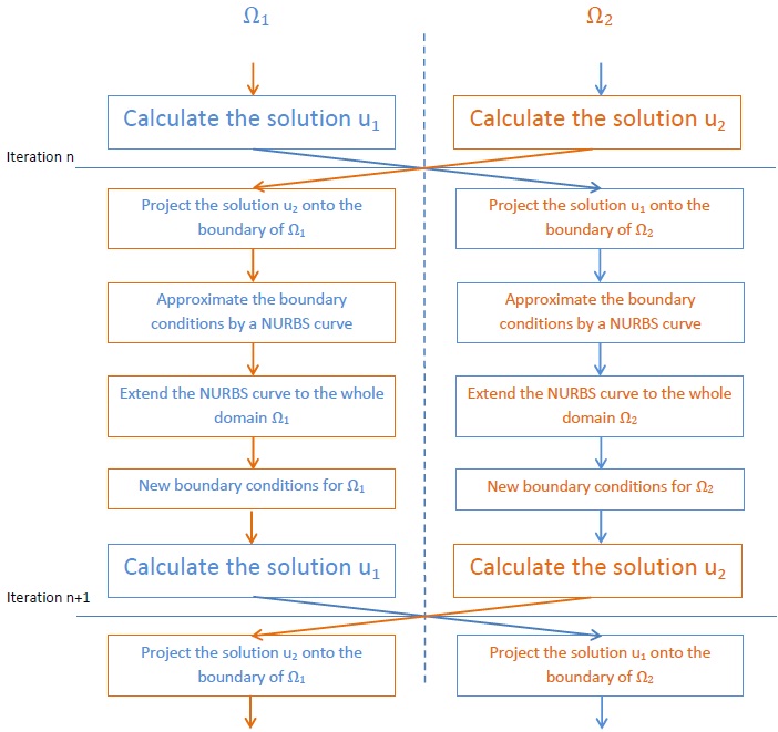
Figure 12: Operations performed on each iterative step in ASDDM with two subdomains $\Omega_{1}$ and $\Omega_{2}$

Figure 12 illustrates the described ASDDM applied to a two domains problem.

13 The Trace Operator

In the present work we consider two ways of projection and compare their performance. Assume that both domains $\Omega_{1}$ and $\Omega_{2}$ are B-spline surfaces with the corresponding piecewise invertible mappings $\mathbf{F}_{1}:\widehat{\Omega}_{1}\rightarrow\Omega_{1}$ and $\mathbf{F}_{2}:\widehat{\Omega}_{2}\rightarrow\Omega_{2}$, where the parametric domains are $\widehat{\Omega}_{1}=\widehat{\Omega}_{2}=[0,1]\times[0,1]$.

13.1 Exact trace operator

We define the exact projetion operator as before:

$$P^{e}_{i}:\mathcal{H}^{1}(\Omega_{j})\rightarrow\mathcal{H}^{1}(\Gamma_{i}^{j})$$

$$u_{j}\rightarrow u_{j}|_{\Gamma_{i}^{j}}.$$

After each iteration on each domain the approximate solution we get is a linear combination of images of B-spline (or NURBS) basis functions. Let us consider the solution $u_{j}^{n-1}$ obtained after $n-1$-th iteration on the subdomain $\Omega_{j}$:

$$u_{j}^{n-1}(x,y)=\sum_{k\in\mathcal{J}}\phi_{k}(x,y){u_{j}}_{k}^{n-1},$$ (13.1.1)

where $\mathbf{u_{j}}=\{{u_{j}}_{i}\}_{i\in\mathcal{J}}$ is the vector of degrees of freedom.

We want to evaluate this function at some point $(x,y)\in\Omega_{j}$. Recall that the pull-back $\mathbf{F}_{j}$ always exists since the geometrical mapping $\mathbf{F}_{j}$ that we use was chosen to be invertible: $(\xi,\eta)=\mathbf{F}_{j}^{-1}(x,y)$. The problem here is that we cannot obtain a closed analytic form of $\mathbf{F}_{j}^{-1}$, which means that in the real computations we will need to use some numerical methods to get the pre-image $(\xi,\eta)$ of the point $(x,y)$.

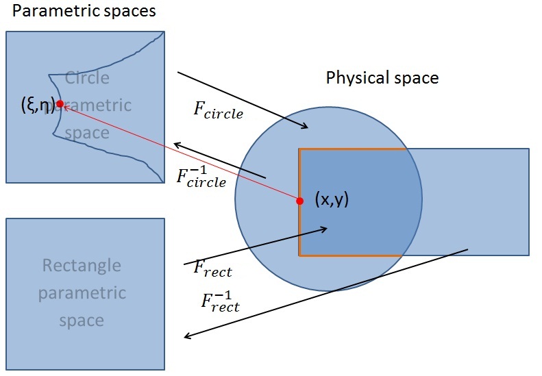
Figure 13: Domains and the pullback $F_{circle}^{-1}(\Gamma_{2}^{1})$ of the boundary $\Gamma_{2}^{1}$

The resulting function $P^{e}_{i}(u_{j}^{n-1})$ is obtained by evaluating the solution $u_{j}^{n-1}$ at any point $(x,y)$ in this way.

In the Figure  13 you can see an example of a pullback of the boundary $\Gamma_{2}$ into the parametric space $\widehat{\Omega}_{1}$

13.2 Interpolation trace operator

The second approach of performing the projection we used was the interpolation trace operator. Given the geometrical mapping $\mathbf{F}$ we can generate a mesh $\mathcal{M}$ in the physical space by applying this mapping to some mesh $\widehat{\mathcal{M}}$ in the parametric space. On the $n$-th iteration we can evaluate the solution $u_{j}^{n},j=1,2$, in the physical domain $\Omega_{j}$ at the mesh points we have just constructed. Our aim is to approximate this solution at any point of the domain $\Omega_{j}$. We obtain it by taking the values of the function $u_{j}^{n}$ in the constructed mesh points and interpolating them into the points of interest, e.g. points on the curve $\Gamma_{i}^{j}$.

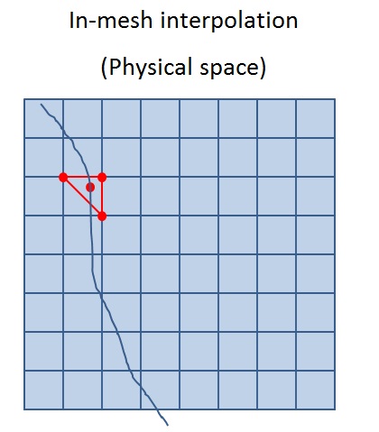
Figure 14: Interpolation projection

There is a wide choice of interpolation methods that we can use. In our research we used linear and cubic interpolations. The interpolation is obtained in the following way: we, first, divide the physical domain into triangles by applying the Delaunay triangulation algorithm to the mesh $\mathcal{M}$. Then for any point $(x,y)\in\Gamma_{i}^{j}$ we define to which triangle it belongs and interpolate the value of the function $u_{j}^{n}$ at this point using the values of this function in the vertices of the triangle we have chosen.

$$P_{i}^{j}:\mathcal{H}^{1}(\Omega_{j})\rightarrow\mathcal{H}^{0}(\Gamma_{i}^{j})$$

$$u_{j}\rightarrow I_{\mathcal{D}}(u_{j}),$$

where $I_{\mathcal{D}}$ is the interpolation operator, depending on the triangulation $\mathcal{D}$ of the mesh $\mathcal{M}$. We will use the notation $P^{l}$ to denote the linear interpolation trace operator.

In the next section we treat a one-dimensional example of ASDDM. We give an overview on the construction of the solver matrices and their structure.

14 One-dimensional ASDDM : Discretized Algorithm

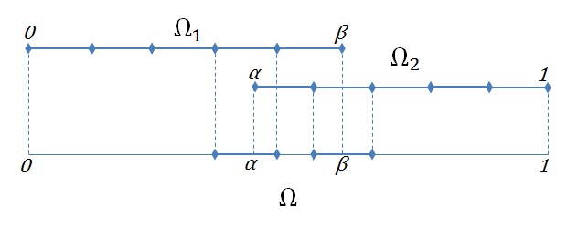
Figure 15: One-dimentional Domain Decomposition

To illustrate the ASDDM on non-matching grids we consider here a simple one-dimensional Poisson equation on a line segment domain $\Omega=[0,1]$.

$$-u_{xx}=f\text{ on }\Omega_{1},u(0)=u(1)=0.$$ (14.0.1)

We decompose the domain into two overlapping domains $\Omega_{1}=[0,\beta)\text{ and }\Omega_{2}=(\alpha,1]$, $\alpha<\beta$ such that $\Omega_{1}\cup\Omega_{2}=\Omega=[0,1]$ as shown in the Figure  15. We assume for convenience that the mapping F is the identity mapping, which implies that we may consider all the equations in the parametric spaces. We denote the knot vectors as $\Xi_{1}=[0,\dots\beta]$ and $\Xi_{2}=[\alpha,\dots 1]$ and the numbers of degrees of freedom as $N_{h1}$ and $N_{h2}$, respectively. Also we assume that the knot vectors are uniform and open and denote the degrees of the polynomials $p_{1}$ and $p_{2}$ on the subdomains $\Omega_{1}$ and $\Omega_{2}$, respectively. To avoid too many indices we denote the solution on $\Omega_{1}$ as $v$ and the solution on $\Omega_{2}$ as $w$.

The two equations which we are going to discretize are:

$$v^{n}_{xx}=f\text{ on }\Omega_{1},v^{n}(0)=0,v^{n}(\beta)=w^{n-1}(\beta).$$ (14.0.2)

$$w^{n}_{xx}=f\text{ on }\Omega_{2},w^{n}(0)=0,w^{n}(\alpha)=v^{n-1}(\alpha).$$ (14.0.3)

The numbering of the basis functions is exactly the same as we used in section  5 .

Consider now the first subdomain $\Omega_{1}$. Only the first basis function $\phi_{1}$ is non-zero at $0$ satisfying $\phi_{1}(0)=1$. In the similar way at the second end of $\Omega_{1}$ $\phi_{N_{h1}}(\beta)=1$ and all the other basis functions vanish at point $\beta$. It means, that in the one-dimensional case the imposition of Dirichlet boundary conditions becomes trivial: we just need to take the first and the last degrees of freedom equal to the projections of the solution on the other subdomain at the boundary points; the approximation operators $A_{i}$ become identities.
Denote the approximate solution on the first subdomain as $\widetilde{v}$ and its vector representation in the B-spline basis as $\mathbf{v}=\{v_{i}\}_{i=1}^{N_{h1}}$. Since the boundary condition at $0$ is constantly zero, the first degree of freedom is $0$: $v_{1}=0$. The treatment of the boundary condition at the point $\beta$ is more involved. We need to project the solution $\widetilde{w}^{n-1}$ of the previous iteration on the second subdomain $\Omega_{2}$ onto the boundary of $\Omega_{1}$ which in our case consists of the only point $\beta$. So we can write $v_{N_{h1}}^{n}=P_{1}(\widetilde{w}^{n-1}(\beta)),$ where $P_{1}$ is the trace operator.

The same reasoning applies on $\Omega_{2}$.

Denote the vector of degrees of freedom of the solution $\widetilde{w}$ as $\mathbf{w}$. The solution $\widetilde{w}^{n-1}$ now reads as

$$\widetilde{w}^{n-1}=\sum_{i=1}^{N_{h2}}\psi_{i}w_{i}^{n-1}.$$

All the operators are acting on finite dimensional spaces, thus they have matrix representations in the basis we have chosen. Since the degree of B-splines on $\Omega_{2}$ is $p_{2}$ we may conclude that there are no more than $p_{2}+1$ non-zero basis functions $\psi_{i}$ at the point $\beta$. As we discussed above, we may use different trace operators in order to project the solution on the subdomain $\Omega_{2}$ onto the boundary $\Gamma_{1}^{2}$ of the subdomain $\Omega_{1}$. In what follows we will consider both cases: the exact trace operator and the interpolation trace operator.

We consider now the two kinds of trace operators we introduced in the previous chapter.

14.1 Exact trace operator $P^{e}$

We take the value $v_{N_{h1}}^{n}$ of the boundary degree of freedom to be equal exactly to the value of the function $\widetilde{w}^{n-1}(\beta)$. For this trivial trace operator, the value $v_{N_{h1}}^{n}$ we get is:

$$v_{N_{h1}}^{n}=(0,\dots,\psi_{i}(\beta),\psi_{i+1}(\beta),\dots,\psi_{i+p_{2}}(\beta),\dots,0)\cdot\begin{pmatrix}0\\ \vdots\\ w_{i}^{n-1}\\ w_{i+1}^{n-1}\\ \vdots\\ w_{i+p_{2}}^{n-1}\\ \vdots\\ 0\end{pmatrix}$$

The operator matrix for the boundary of the $\Omega_{1}$ subdomain is:

$$P^{e}_{1}=\begin{pmatrix}0&\dots&0&0&\dots&0&\dots&0\\ 0&\dots&0&0&\dots&0&\dots&0\\ \vdots&\dots&\vdots&\vdots&\dots&\vdots&\dots&\vdots\\ 0&\dots&\psi_{i}(\beta)&\psi_{i+1}(\beta)&\dots&\psi_{i+p_{2}}(\beta)&\dots&0\end{pmatrix},$$

where $P^{e}_{1}\in\mathbb{R}^{N_{h1}\times N_{h2}}.$

Denote by $A_{1}$ the stiffness matrix for the first subdomain. As before, we partition the sets of indices of basis functions $\mathcal{J}=\{1,2,\dots,N_{hj}\},j=1,2$ into two subsets. The subset $\mathcal{I}\subset\mathcal{J}$ of the inner degrees of freedom and $\mathcal{B}\subset\mathcal{J}$ of the boundary degrees of freedom. In the one dimensional case $\mathcal{B}=\{1,N_{hj}\}$ and $\mathcal{I}=\mathcal{J}\backslash\{1,N_{hj}\}=\{2,3,\dots,N_{hj}-1\},j=1,2.$ So the restriction of the stiffness matrix corresponding to the inner degrees of freedom reads as $A_{1}(\mathcal{I},\mathcal{I})$.

Since the basis functions are not local, when we impose the Dirichlet boundary conditions on some of the degrees of freedom, we need to subtract the function $v_{N_{h1}}^{n}\phi(\xi)$ from the solution $\widetilde{v}^{n}$. We do it by subtracting the corresponding values from the degrees of freedom of the basis functions $\{\phi\}_{i=N_{h1}-k}^{N_{h1}}$ which domain intersects with the domain of $\phi_{N_{h1}}$. Now the discretized equation for the subdomain $\Omega_{1}$ can be rewritten as:

$$\begin{split}&\begin{pmatrix}1&0&\dots&0&0\\ 0&&A_{1}(\mathcal{I},\mathcal{I})&&0\\ 0&0&\dots&0&1\end{pmatrix}\cdot\mathbf{v}^{n}=\begin{pmatrix}0\\ \mathbf{f_{1}}\\ 0\end{pmatrix}+\begin{pmatrix}1&\dots&0\\ &-A_{1}(\mathcal{I},\mathcal{B})&\\ 0&\dots&1\end{pmatrix}\cdot\\ &\cdot\begin{pmatrix}0&\dots&0&0&\dots&0&\dots&0\\ 0&\dots&0&0&\dots&0&\dots&0\\ \vdots&\dots&\vdots&\vdots&\dots&\vdots&\dots&\vdots\\ 0&\dots&\psi_{i}(\beta)&\psi_{i+1}(\beta)&\dots&\psi_{i+p_{2}}(\beta)&\dots&0\end{pmatrix}\cdot\mathbf{w}^{n-1},\\ \end{split}$$ (14.1.1)

where the vector $\mathbf{f_{1}}$ corresponds to the inner degrees of freedom of the first subdomain. Exactly the same reasoning can be applied to the second subdomain $\Omega_{2}$ to get the following discretized equation:

$$\begin{split}&\begin{pmatrix}1&0&\dots&0&0\\ 0&&A_{2}(\mathcal{I},\mathcal{I})&&0\\ 0&0&\dots&0&1\end{pmatrix}\cdot\mathbf{w}^{n}=\begin{pmatrix}0\\ \mathbf{f_{2}}\\ 0\end{pmatrix}+\begin{pmatrix}1&\dots&0\\ &-A_{2}(\mathcal{I},\mathcal{B})&\\ 0&\dots&1\end{pmatrix}\cdot\\ &\cdot\begin{pmatrix}0&\dots&\phi_{j}(\alpha)&\phi_{j+1}(\alpha)&\dots&\phi_{j+p_{1}}(\alpha)&\dots&0\\ \vdots&\dots&\vdots&\vdots&\dots&\vdots&\dots&\vdots\\ 0&\dots&0&0&\dots&0&\dots&0\\ 0&\dots&0&0&\dots&0&\dots&0\\ \end{pmatrix}\cdot\mathbf{v}^{n-1}.\\ \end{split}$$ (14.1.2)

Let us denote the vector of degrees of freedom of the “whole” approximate solution $\widetilde{u}^{n}$ as $\mathbf{u}^{n}=\begin{pmatrix}\mathbf{v}^{n}\\ \mathbf{w}^{n}\end{pmatrix}$. Now, we can unite the two equations (14.1.1) and (14.1.2) into a single matrix equation

$$A\cdot\mathbf{u}^{n}=f+A_{dir}\cdot P\cdot\mathbf{u}^{n-1},$$ (14.1.3)

where

$$A=\begin{pmatrix}\begin{matrix}1&\dots&0\\ 0&A_{1}(\mathcal{I},\mathcal{I})&0\\ 0&\dots&1\\ \end{matrix}&O\\ O&\begin{matrix}1&\dots&0\\ 0&A_{2}(\mathcal{I},\mathcal{I})&0\\ 0&\dots&1\\ \end{matrix}\end{pmatrix}=\begin{pmatrix}\tilde{A}_{1}&O\\ O&\tilde{A}_{2}\end{pmatrix},$$

with $\tilde{A}_{1}\in\mathbb{R}^{N_{h1}\times N_{h1}},\tilde{A}_{2}\in\mathbb{R}^{N_{h2}\times N_{h2}},$

$$f=\begin{pmatrix}0\\ \mathbf{f_{1}}\\ 0\\ 0\\ \mathbf{f_{2}}\\ 0\\ \end{pmatrix},$$

$$A_{dir}=\begin{pmatrix}\begin{matrix}1&\dots&0\\ &-A_{1}(\mathcal{I},\mathcal{B})&\\ 0&\dots&1&\\ \end{matrix}&O\\ O&\begin{matrix}1&\dots&0\\ &-A_{2}(\mathcal{I},\mathcal{B})&\\ 0&\dots&1\\ \end{matrix}\end{pmatrix}=\begin{pmatrix}\widetilde{A}_{dir1}&O\\ O&\widetilde{A}_{dir2}\end{pmatrix},$$

with $\widetilde{A}_{dir1}\in\mathbb{R}^{N_{h1}\times N_{h1}},\widetilde{A}_{dir2}\in\mathbb{R}^{N_{h2}\times N_{h2}},$

$$\begin{split}&P=\begin{pmatrix}O&\begin{matrix}0&\dots&0&\dots&0&\dots&0\\ 0&\dots&0&\dots&0&\dots&0\\ \vdots&\dots&\vdots&\dots&\vdots&\dots&\vdots\\ 0&\dots&\psi_{i}(\beta)&\dots&\psi_{i+p_{2}}(\beta)&\dots&0\\ \end{matrix}\\ \begin{matrix}0&\dots&\phi_{j}(\alpha)&\dots&\phi_{j+p_{1}}(\alpha)&\dots&0\\ \vdots&\dots&\vdots&\dots&\vdots&\dots&\vdots\\ 0&\dots&0&\dots&0&\dots&0\\ 0&\dots&0&\dots&0&\dots&0\\ \end{matrix}&O\end{pmatrix}\\ &=\begin{pmatrix}O&\tilde{P}_{1}\\ \tilde{P}_{2}&O\end{pmatrix},\end{split}$$ (14.1.4)

with $P_{1}^{e}\in\mathbb{R}^{N_{h1}\times N_{h2}},P_{2}^{e}\in\mathbb{R}^{N_{h2}\times N_{h1}}.$

The iterative scheme is given by:

$$\begin{split}&\begin{pmatrix}\tilde{A}_{1}&O\\ O&\tilde{A}_{2}\end{pmatrix}\cdot\mathbf{u}^{n}=f+\begin{pmatrix}\widetilde{A}_{dir1}&O\\ O&\widetilde{A}_{dir2}\end{pmatrix}\cdot\begin{pmatrix}O&P_{1}^{e}\\ P_{2}^{e}&O\end{pmatrix}\cdot\mathbf{u}^{n-1}=\\ &f+\begin{pmatrix}O&\widetilde{A}_{dir1}P_{1}^{e}\\ \widetilde{A}_{dir2}P_{2}^{e}&O\end{pmatrix}\cdot\mathbf{u}^{n-1},\end{split}$$ (14.1.5)

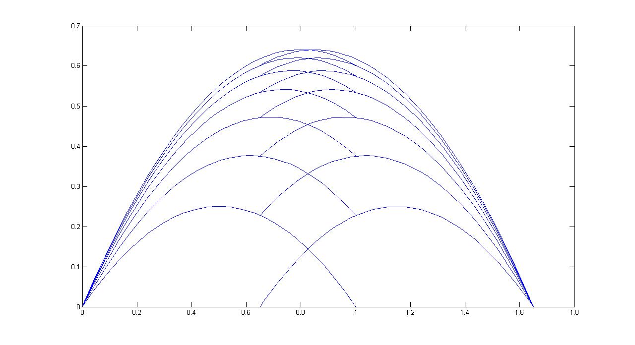
Figure 16: One-dimensional Schwarz Method for the equation $u_{xx}=-1$, using the exact trace operator $P^{e}$ and zero initial guesses

Figure 17: One-dimensional Schwarz Method for the equation $u_{xx}=-1$, using the linear interpolation trace operator $P^{l}$ and zero initial guesses

We emphasize here that the matrix

$$\begin{pmatrix}\tilde{A}_{1}&O\\ O&\tilde{A}_{2}\end{pmatrix}$$ (14.1.6)

is not symmetric since the domains may have different number of elements, or even different orders of approximation.

14.2 Linear interpolation trace operator

We consider here the linear interpolation operator we discussed in the previous chapter.

The algorithm works as was explained above: consider the first subdomain $\Omega_{1}=[0,\beta)$. In order to construct a linear interpolation of the solution $\widetilde{w}^{n-1}$ at the point $\eta=\beta$ we need to find the knot span $[\eta_{i},\eta_{i+1})$ which contains $\beta$. We take the values of the function $\widetilde{w}^{n-1}$ at the ends of this chosen span interval $\widetilde{w}^{n-1}(\eta_{i})$ and $\widetilde{w}^{n-1}(\eta_{i+1})$ and their weighted sum:

$$v_{N_{h1}}^{n}=\frac{\beta-\eta_{i}}{\eta_{i+1}-\eta_{i}}\widetilde{w}^{n-1}(\eta_{i})+\frac{\eta_{i+1}-\beta}{\eta_{i+1}-\eta_{i}}\widetilde{w}^{n-1}(\eta_{i+1}).$$

We see that the linear interpolation trace operator is, actually, a convex sum of the two exact interpolation operators corresponding to the points $\eta_{i}$ and $\eta_{i+1}$:

$$P_{1}^{l}=\frac{\beta-\eta_{i}}{\eta_{i+1}-\eta_{i}}P^{e}(\eta_{i})+\frac{\eta_{i+1}-\beta}{\eta_{i+1}-\eta_{i}}P^{e}(\eta_{i+1}).$$ (14.2.1)

Consequently, the matrix of this interpolation trace operator can be obtained as the convex sum of the matrices of the exact trace operators at the points $\eta_{i}$ and $\eta_{i+1}$.

$$\begin{split}&P_{1}^{l}=\frac{\beta-\eta_{i}}{\eta_{i+1}-\eta_{i}}\begin{pmatrix}0&\dots&0&0&\dots&0&\dots&0\\ 0&\dots&0&0&\dots&0&\dots&0\\ \vdots&\dots&\vdots&\vdots&\dots&\vdots&\dots&\vdots\\ 0&\dots&\psi_{i}(\eta_{i})&\psi_{i+1}(\eta_{i})&\dots&\psi_{i+p_{2}}(\eta_{i})&\dots&0\end{pmatrix}\\ &+\frac{\eta_{i+1}-\beta}{\eta_{i+1}-\eta_{i}}\begin{pmatrix}0&\dots&0&0&\dots&0&\dots&0\\ 0&\dots&0&0&\dots&0&\dots&0\\ \vdots&\dots&\vdots&\vdots&\dots&\vdots&\dots&\vdots\\ 0&\dots&\psi_{i+1}(\eta_{i+1})&\psi_{i+2}(\eta_{i+1})&\dots&\psi_{i+p_{2}+1}(\eta_{i+1})&\dots&0\end{pmatrix}.\end{split}$$ (14.2.2)

The iterative scheme is now:

$$\begin{split}&\begin{pmatrix}\tilde{A}_{1}&O\\ O&\tilde{A}_{2}\end{pmatrix}\cdot\mathbf{u}^{n}=f+\begin{pmatrix}\widetilde{A}_{dir1}&O\\ O&\widetilde{A}_{dir2}\end{pmatrix}\cdot\begin{pmatrix}O&P_{1}^{l}\\ P_{2}^{l}&O\end{pmatrix}\cdot\mathbf{u}^{n-1}=\\ &f+\begin{pmatrix}O&\widetilde{A}_{dir1}P_{1}^{l}\\ \widetilde{A}_{dir2}P_{2}^{l}&O\end{pmatrix}\cdot\mathbf{u}^{n-1},\end{split}$$ (14.2.3)

where

$$P_{2}^{l}=\frac{\alpha-\xi_{j}}{\xi_{j+1}-\xi_{j}}P^{e}(\xi_{j})+\frac{\xi_{j+1}-\alpha}{\xi_{j+1}-\xi_{j}}P^{e}(\xi_{j+1}).$$ (14.2.4)

and $\alpha$ belongs to the knot span $[\xi_{j},\xi_{j+1})$.

14.3 Initial guesses

Of course, there is some freedom in choosing the initial boundary values $\widetilde{v}^{0}(\beta)$ and $\widetilde{w}^{0}(\alpha)$. It turns out that the method converges to the same approximate solutions regardless of the initial guesses since the convergence is guaranteed by the properties of the matrix, which is a M-matrix in our case as shown in the Appendix.

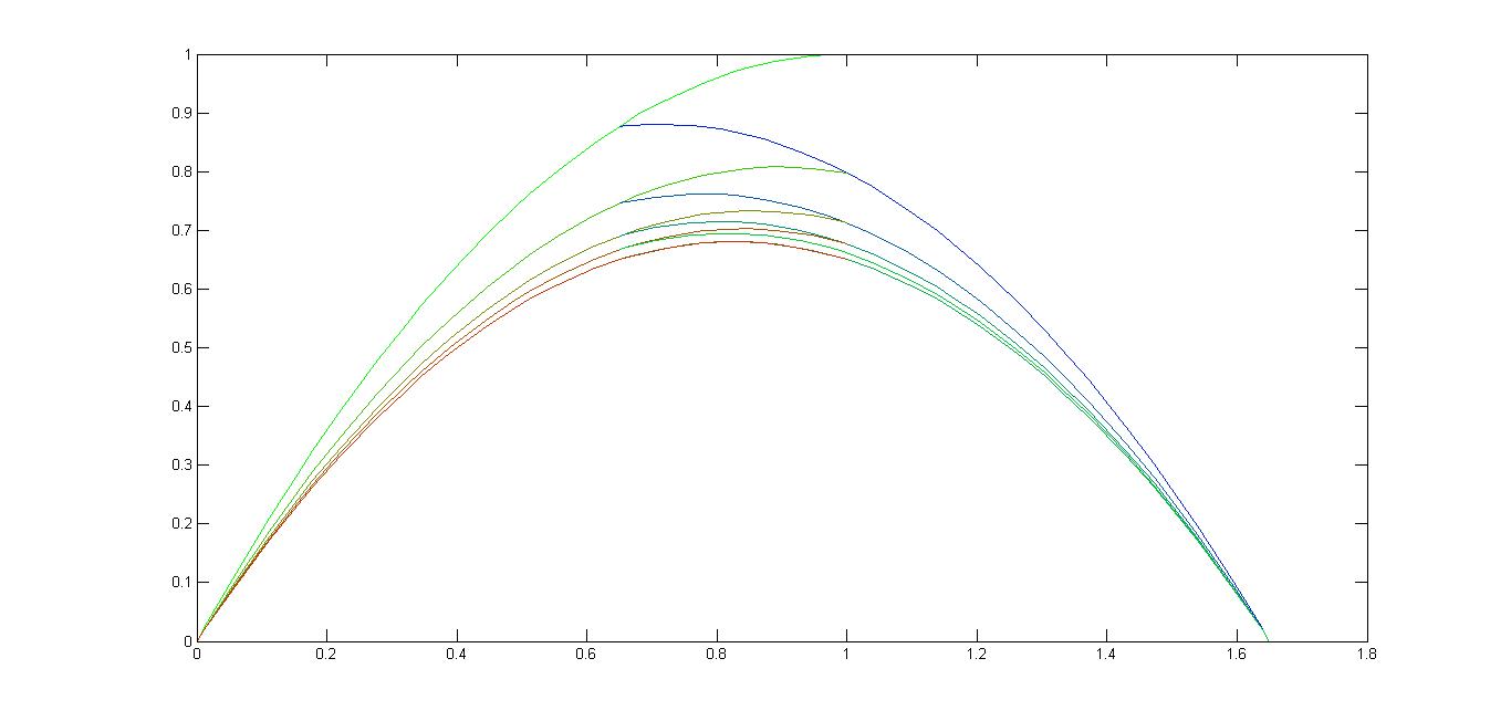
Figure 18: Convergence of the one-dimensional SADDM with non-zero initial guesses. Here the initial values for the inner boundary points are taken $\widetilde{v}^{0}(\beta)=\beta$ and $\widetilde{w}^{0}(\alpha)=\alpha$

You can see an example of a convergence procedure for non-zero initial guesses in the Figure 18

14.4 Multi-dimensional domains

When we consider a multi - dimensional case we have to perform an approximation of the boundary conditions since the boundary condition function is be a B-spline or NURBS curve or surface in general. This approximation can be performed in one of the ways we have already discussed above in section  7 : quasi-interpolation or least-squares approximation. All the other steps of the solution are similar to the one-dimensional case.
In the next chapter we consider two and three dimensional applications of ASDDM as well as its parallelisation.

15 Numerical Results

In this section we provide illustration of the convergence properties of the ASDDM in our implementation. As we have already mentioned one of the main advantages of the ASDDM methods is that the meshes of different patches are non-matching. This important feature makes it possible to apply this method in CSG and zooming problems. In particular, it allows to perform local zooming at places where the solution possesses weak singularities. Below we demonstrate some examples of this technique and its usage. We also describe how we implement the parallelized version of the solver and show a few three-dimensional multi-patched examples obtained with it.

As already mentioned before in all the model problems considered in this work the errors are $\mathcal{L}^{2}$-norm differences between the exact solutions and the approximations, see section (4.1.2).

16 One-dimensional examples and Analysis

16.1 Dependence of the convergence on the B-spline degree

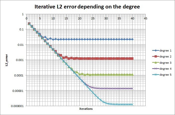
Figure 19: $\mathcal{L}^{2}$-error iterative convergence depending on the polynomial degree, one-dimensional case.

First, we treat the one-dimensional problem to show how the iterative process depends on the degree of the B-splines used. The graph given in Figure 19 shows the $\mathcal{L}^{2}$-errors as a function of the iteration number for different polynomial degrees. Obviously, higher polynomial degrees lead to better precision of the final result, but the rates of convergence remain the same which makes the iterative procedure time consuming.

16.2 Dependence of the convergence on the overlapping area

Many times when the Domain Decomposition technique is applied to the original domain we have some freedom in choosing the subdomains. For example, when a local zooming is considered the only thing which is predefined is the domain we zoom in, but the choice of the second subdomain is given to us. The question is how the relative overlapping area influences the convergence process. In Figure  20 we compare different domain decompositions for the same one-dimensional example. The overlapping is measured as the ratio of the overlapping area to the area of one subdomain. Apparently, the larger the overlapping is, the faster the iterative convergence becomes. An open question is how would one balance the overlapping and the number of degrees of freedom versus the number of iterations to optimize the computation.

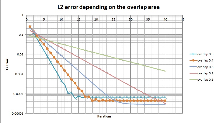
Figure 20: $\mathcal{L}^{2}$-error iterative convergence depending on the ovrelapping area

16.3 Dependence of the approximate solution on the mesh size

Figure  21 shows how the approximate solution depends on the refinement for different degrees of B-splines. You can see that the dependence is close to theoretically predicted, given by the formula  [15]:

$$\inf_{s\in\mathcal{V}}||u\circ\mathbf{F}-s||_{\mathcal{L}^{2}}\leq Ch^{p+1}|u\circ\mathbf{F}|_{\mathcal{H}^{p+1}},$$ (16.3.1)

where $u$ is the exact solution and $C$ is a constant that may depend on the degree $p$ of the polynomials.

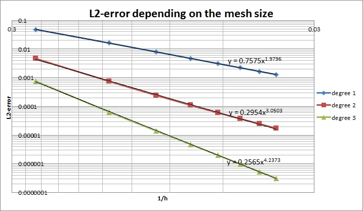
Figure 21: One-dimensional $\mathcal{L}^{2}$-error of the approximate solution depending on the mesh size for different polynomial degrees

17 Convergence properties in multi-dimensional cases: Application to Zooming

The formula 16.3.1 becomes different in the multi-dimensional case, but still the approximated solution depends on the mesh size in almost the same way [15].

Consider the following two-dimensional problem:

Let $\Omega$ be an open circle of radius 3 placed at the origin:

$$-\Delta u=\sin(x^{2}+y^{2}-9)-4\cos(x^{2}+y^{2}-9)\text{ on }\Omega,$$ (17.0.1)

$$u|_{\partial\Omega=0}.$$ (17.0.2)

The exact solution is $u=\sin(x^{2}+y^{2}-9)$

Apply zooming by considering $\Omega$ as a union of an annulus and a square. $\Omega=\Omega_{annulus}\cup\Omega_{square}$ as shown in the Figure 22.

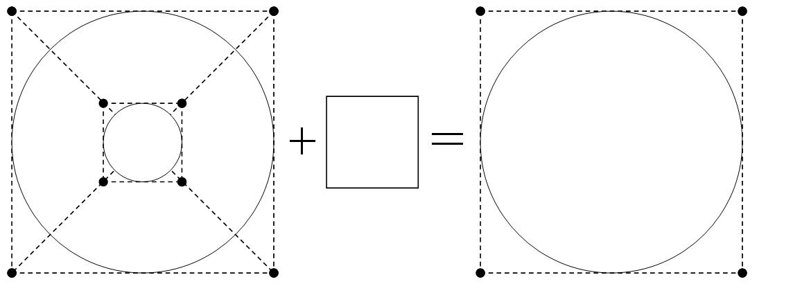
Figure 22: Domain Decomposition scheme

In Figures 23 and 24 below you can see the convergence properties and the numerical solutions we obtained in this case by applying the ASDDM.

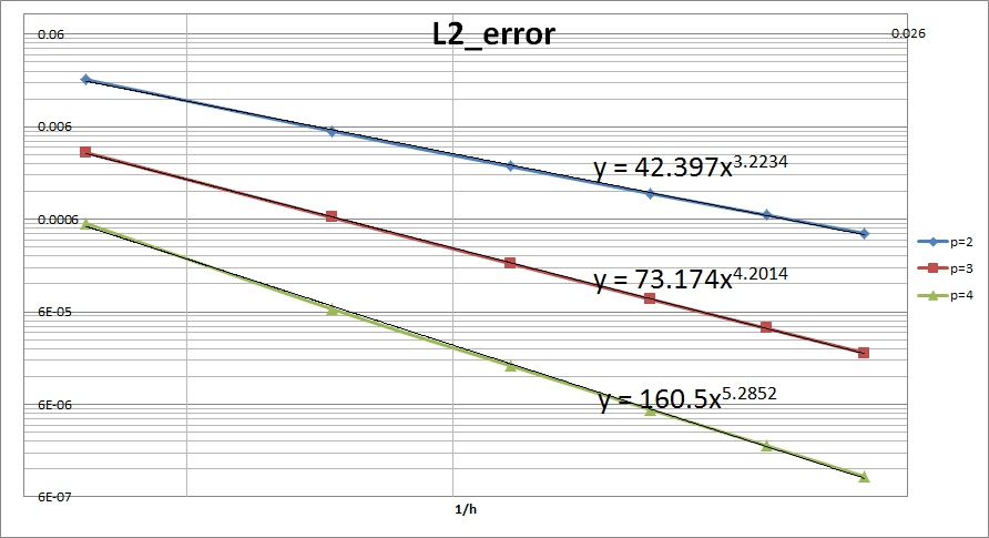
Figure 23: Annulus $\mathcal{L}^{2}$-errors depending on the mesh size for different polynomial degrees

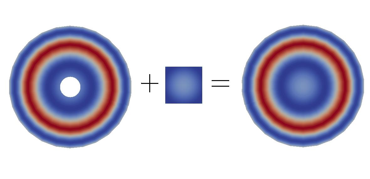
Figure 24: Numerical solution

18 Two-dimensional examples

18.1 Non-matching domain meshes

An example of non-matching meshes and a solution obtained by the Domain Decomposition method is shown in Figure 25. The domain is taken from the logo of the Domain Decomposition organization, seeFigure  11. We also give in Table 1 the reaction between overlap and DD iterations.

Table 1: Number of Iteration and max error by Overlap Distance

Overlapp	$0.1$	$0.25$	$0.5$	$0.75$	$1.0$
Iterations	max error	at each iteration
1	$.6*10^{-1}$	$.9*10^{-1}$	$1.2*10^{-1}$	$1.2*10^{-1}$	$0.7*10^{-1}$
2	$.3*10^{-1}$	$.3*10^{-1}$	$0.16*10^{-1}$	$0.12*10^{-1}$	$0.11*10^{-1}$
3	$.15*10^{-1}$	$.024*10^{-1}$	$0.01*10^{-1}$	$0.01*10^{-1}$	$0.022*10^{-1}$
4	$.05*10^{-1}$	$.08*10^{-1}$	$0.034*10^{-1}$	$0.005*10^{-1}$	$0.006*10^{-1}$
5	$.03*10^{-1}$	$.007*10^{-1}$	$0.006*10^{-1}$	$0.006*10^{-1}$	$0.001*10^{-1}$
6	$.02*10^{-1}$	$.004*10^{-1}$	$0.002*10^{-1}$	$0.003*10^{-1}$	$c$
7	$.02*10^{-1}$	$.002*10^{-1}$	$0.0015*10^{-1}$	$0.002*10^{-1}$	$c$
8	$.01*10^{-1}$	$.002*10^{-1}$	$0.001*10^{-1}$	$0.001*10^{-1}$	$c$
9	$.006*10^{-1}$	$.001*10^{-1}$	$c$	$c$	$c$
10	$.003*10^{-1}$	$c$	$c$	$c$	$c$

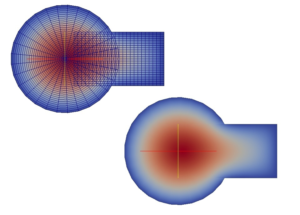
Figure 25: Numerical solution over the DD logo.

18.2 Application of zooming: weak corner singularity

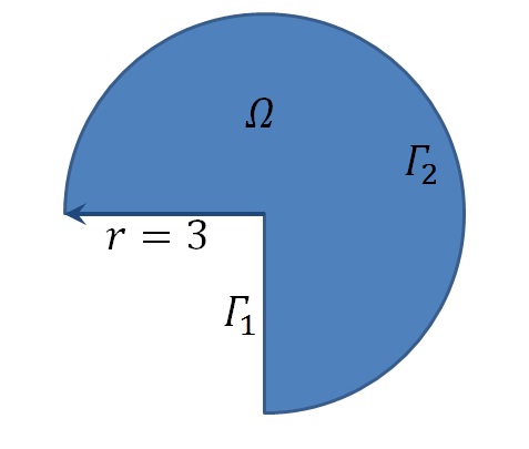
Figure 26: Problem with a weak singularity at the corner. The domain.

We now consider some engineering applications of the Domain Decomposition techniques used for zooming. One of the main applications of ASDDM are the problems where the solution possesses a weak singularity at the corner. The example we treat here is taken from [7].

Given the following domain:

$$\Omega=\{(\rho,\theta)\in\mathbb{R}|0<\rho<3;-\frac{\pi}{2}<\theta<\pi\},$$ (18.2.1)

which is an open circular sector of angle $\alpha=\frac{3\pi}{2}$ as shown in Figure 26 and the equation:

$$\Delta u=0\text{ in }\Omega,$$ (18.2.2)

$$u=\left\{\begin{array}[]{ll}0&:\text{on }\Gamma_{1}\subset\Gamma_{\Omega}=\partial{\Omega}\\ \theta(\alpha-\theta)&:\text{on }\Gamma_{2}=\Gamma_{\Omega}\backslash\Gamma_{1}.\end{array}\right.$$

The exact solution is given by the following uniformly convergent series:

$$u_{ex}(\rho,\theta)=\frac{9}{\pi}\sum_{n=1,3,5,\dots}\frac{1}{n^{3}}\left(\frac{\rho}{r}\right)^{\frac{2n}{3}}\sin\left(\frac{2n\theta}{3}\right).$$ (18.2.3)

We see from  (18.2.3) that the radial derivative is unbounded when approaching the origin which may cause the numerical solution to be unstable at the vicinity of the origin. In order to zoom the solution near the corner we decompose the domain in the following way: $\Omega=\Omega_{out}\cup\Omega_{zoom},$ as shown in Figure 27.

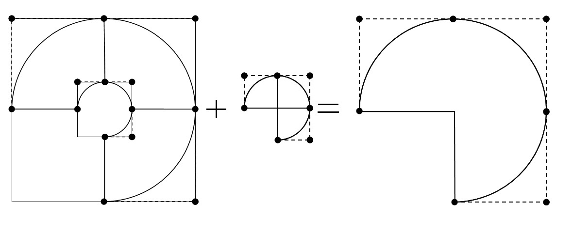
Figure 27: NURBS definition, Boundary and Domain Decomposition

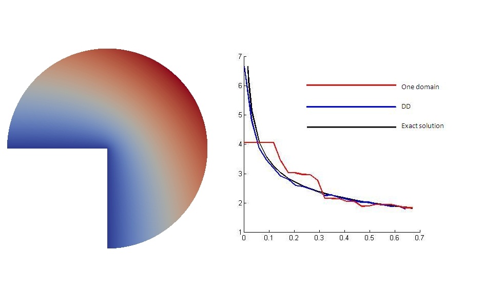
Figure 28: Numerical solution of (3.2) and the corresponding radial derivative

Figure 28 shows the numerical solution and the radial derivative calculated for this problem. The principal order of the radial derivative of the exact solution is $-\frac{1}{3}$, and the numerically computed result using the Domain Decomposition technique coincides with this value.

We have tested different forms of the zooming region as shown in Figure 29 and in all the cases the results coincided.

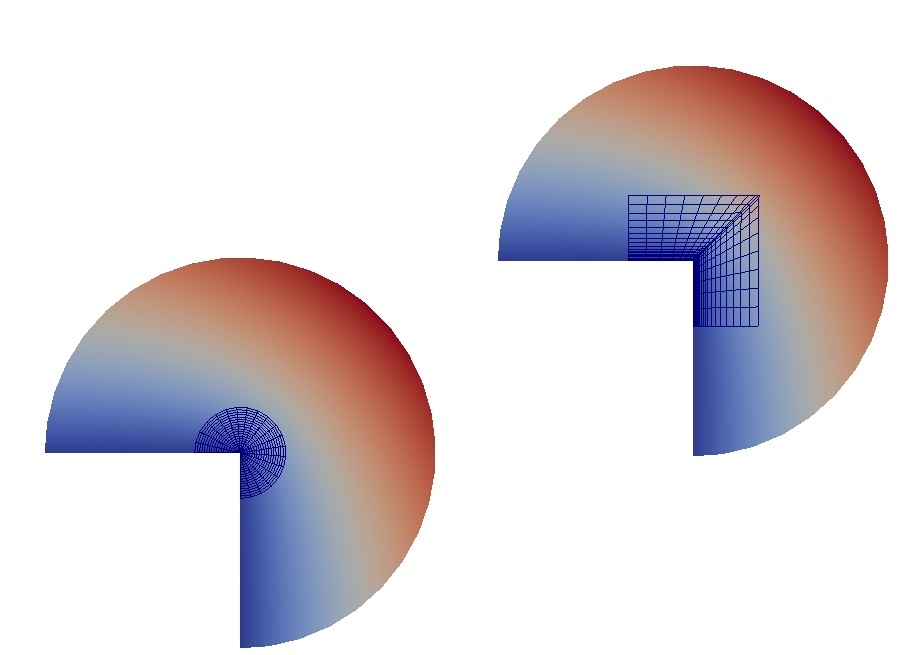
Figure 29: Different zooming regions

The solution in this case is not regular and possesses a weak singularity at the corner and the error estimate 16.3.1 does not apply anymore. The dependence of the approximate solution on the mesh size becomes different from the regular case and the rate of convergence does not improve with greater polynomial degree as shown in Figure  30.

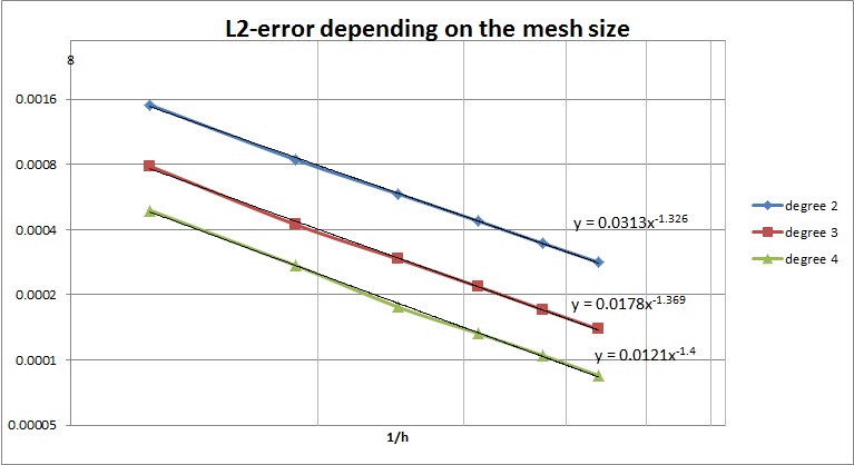
Figure 30: $\mathcal{L}^{2}$-error of the approximate solution depending on the mesh size for different polynomial degrees

19 Three-dimensional examples

In this section we present some examples obtained for multi-patched bodies. Consider the equation:

$$-\Delta u=\sin(x+y+z)\text{ on }\Omega,$$ (19.0.1)

$$u|_{\partial\Omega}=\sin(x+y+z),$$ (19.0.2)

where $\Omega$ is a chain of 5 overlapping cubes, as shown in Figure 31. The exact solution is $u=\sin(x+y+z)$. You can see the rates of convergence of the solution for all the 5 cubes in the Figure 32.

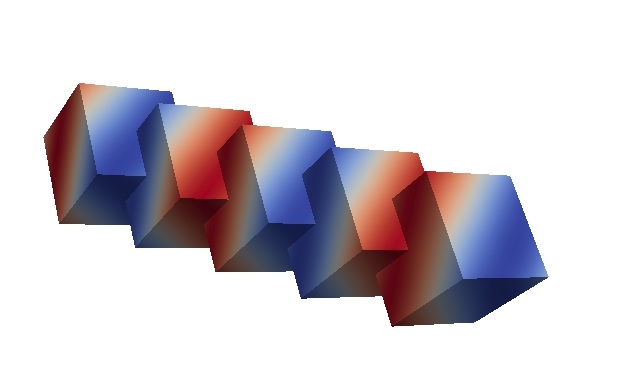
Figure 31: Chain of cubes with the exact solution $\sin(x+y+z)$

Figure 32: Iterative $\mathcal{L}^{2}$-error for the chain of cubes

19.1 Parallelized algorithm and multi-patched problems

As we have mentioned in the beginning of this work, one of the main advantages of the ASDDM is that it may be easily parallelized. The modern computers are all multi-core which provides us with an opportunity of real parallelization of the code, meaning that the solution on each patch may be computed independently and simultaneously on a different processor.

The algorithm we implemented works as following. Before we start the iterations we precompute all the date that the solver needs, then we open a worker thread for each subprocess, corresponding to a patch, and start the iterative procedure. On each iteration the $n$-th thread solves the equation on the $n$-th subdomain according to the scheme shown in Figure 12 of the previous chapter. After the $n$-th iteration computation is finished, the data is synchronized between the threads. This synchronization is necessary to impose the correct boundary conditions for each subdomain on the next iteration.

The schematic synchronization mechanism is shown in Figure 33.

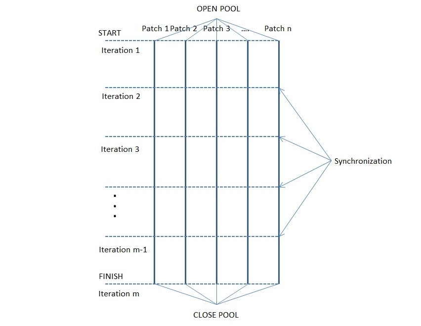
Figure 33: Synchronization algorithm

19.2 Elasticity example for multi-patched domain

As an example of parallel computation we took an elasticity problem. The domain is a hollow thick half-ring with fixed ends which is placed into a gravitational field. This patch was decomposed into 8 overlapping subdomains as shown in the Figure 34 and the solution was obtained using the parallelized method described above.

We performed numerical tests on the 4-processors machine and achieved a full 4-times enhancement in the time of computations.

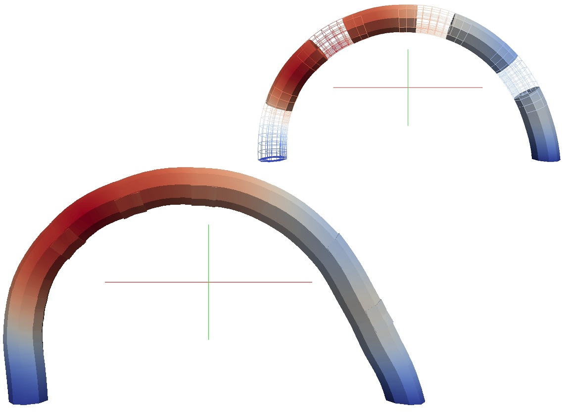
Figure 34: Elasticity example

19.3 Statistics

In this section we illustrate the dependence of the number of degrees of freedom in the problem as a function of dimension, refinement and polynomial degrees. Of course, these numbers do not depend on the isogeometrical mapping, so we calculated the data using a cube domain.

In the two-dimensional case we obtained:

degree of the B-splines
Partitions of the mesh	$2$	$3$	$4$
0	10	27	52
1	27	52	85
2	52	85	126
5	175	232	297
10	540	637	742
11	637	742	855
20	1870	2047	2232

In the three-dimensional case we obtained:

degree of the B-splines
Partitions of the mesh	$1$	$2$
1	765	624
2	2100	1275

The number of degrees of freedom, and consequently, the computational time grows rapidly with the dimension of the problem, especially if the mesh need to be refined. Here the Domain Decomposition techniques become very helpful.

20 Conclusion

The main purpose of this work was to establish the connection and application of the recently discovered IGA framework to solve PDEs using Additive Domain Decomposition Method. It turns out that IGA may be successfully used for solving different problems even on complex geometries, thus giving us all the advantages of IGA without restrictions on the geometry. Another important application of these methods are zooming problems. The IGA framework is restricted to its native techniques like T-splines and here the Domain Decomposition becomes very useful.

More research is needed is to explore ways of approximating and imposing the Dirichlet boundary conditions. Different techniques of imposing boundary conditions may influence the computational times and the precision of the approximate solution significantly hence a research subject is improving techniques to define such BCs on trimmed patches.

The question of optimal overlap choice ( a large overlap seems better, but more costly in degrees of freedom) needs more study. Also what is the best way to define the solution on the intersections is an opened question.

Another important direction for research is the preconditioning of the solver in large scale problems. An efficient pre-conditioner may improve the computational times and simplify the structure of the solver( and insure convergence , since we do not have a maximum principle here.)

Finally a CSG construct is not made only of unions of primitives, and it my be the results of Boolean differences, substractions etc.,thus DD should be coupled with other methods such as fictitious domains .

References

- [1] Toselli A. and Widlund O. B. Domain Decomposition Methods :Algorithms and Theory, volume 34 of Computational Mathematics. Springer Verlag, 2004.
- [2] I. Harari I A. Embar, J. Dolbow. Imposing dirichlet boundary conditions with nitsche’s method and spline-based finite elements (article). International Journal for Numerical Methods in Engineering, 83:877–898, 2010.
- [3] Pavarino L. F. Scacchi S. Beirao da Veiga L., Cho D. Overlapping schwarz methods for isogeometric analysis. SIAM Journal of Numerical Analysis, 50(3):1394–1416, 2012.
- [4] R. Vázquez C. de Falco, A. Reali. Geopdes: a research tool for isogeometric analysis of pdes. Advances in Engineering Software, 42(12):1020–1034, 2011.
- [5] H. Speleers C. Manni. Standard and non-standard cagd tools for isogeometric analysis: a tutorial ,. Technical Report TW642, KU Leuven, Dept. Comput. Science,, 2014.
- [6] P. G. Ciarlet. Numerical Analysis of the Finite Element Method. Les Presses de L’Universite de Montreal, Quebec, Canada, 1976.
- [7] J. B. Keller D. Givoli, L. Rivkin. A finite element for domains with corners. International Journal for Numerical Methods in Engineering, 1329-1335:pp. 1329 − 1345, 1992.
- [8] Juttler B. Dorfel M. R. and Simeon B. Adaptive isogeometric analysis by local h-refinement with t-splines. Computer Methods in Applied Mechanics and Engineering, 199:264–276, 2010.
- [9] Steger J.L. Dougherty F. C. and Benek J.A. A chimera grid scheme. In K. N. Chis and U. Ghia, editors, Advances in Grid Generation, volume FED 5. ASME, 1983.
- [10] C. Giannelli G.Kiss and B. Juttler. Algorithms and data structures for truncated hierarchical b–splines. In M.Floater et al., editor, Mathematical Methods for Curves and Surfaces, number 8177 in Lecture Notes in Computer Science, pages 304–323. Springer, 2014.
- [11] Mitchell T. J. Govindjee S., Strain J. and Taylor R. L. Convergence of an efficient local least-squares fitting method for bases with compact support, comput. methods appl. mech. engrg., pp 84-92, 2012. Computer Methods in Appl. Mech. and Eng., 213-216:84–92, 2012.
- [12] Schwarz H.A. √úber einen grenz√ºbergang durch alternierendes verfahren,. Vierteljahrsschrift der Naturforschenden Gesellschaft in Zurich, 15: pp. 272-286, 1870., 15:272–286, 1870.
- [13] Lions J.-L. and Magenes E. Problemes aux limites non homognes et applications,, volume 1,2. Dunod., Paris, vol. 1, 2, 1968.
- [14] Y Bazilevs J.A. Cottrell, T.J.R. Hughes. Isogeometric Analysis: toward integration of CAD and FEA. Wiley, 2009.
- [15] G. Sangalli R. Vázquez. L. Beirão da Veiga, A. Buffa. Mathematical analysis of variational isogeometric methods. Acta Numerica, 23(157-287), 2014.
- [16] S. Scacchi O.B. Widlund S. Zampini L. Beirão da Veiga, L.F. Pavarino. Isogeometric bddc preconditioners with deluxe scaling. SIAM J. Sci. Comput., 36(3):A1118–A1139, 2014.
- [17] P.L. Lions. On the schwarz alternating method,. In R. Glowinski et al., editor, First International Symposium on Domain Decomposition Methods for Partial Differential Equations,, pages 1–44. SIAM, 1988.
- [18] Hofmann C. M. Geometric and solid modeling,. Morgan Kaufmann, San Mareo, CA., http://www.cs.purdue.edu/homes/cmh/distribution/books/geo.htm, 1989.
- [19] L. Piegl and W. Tiller. The NURBS Book. Monographs in Visual Communication. Springer, Wellesley, MA, second edition, 1997.
- [20] V.M. Calo et al. Y. Bazilevs. Isogeometric analysis using t-splines. Computer Methods in Appl. Mech. and Eng., 199(5-8):229–263, January 2010.