A lava attack on the recovery of sums of dense and sparse signals

Victor Chernozhukov Department of Economics, MIT, Cambridge, MA 02139 vchern@mit.edu Christian Hansen Booth School of Business, University of Chicago, Chicago, IL 60637 Christian.Hansen@chicagobooth.edu  and  Yuan Liao Department of Mathematics, University of Maryland, College Park, MD 20741 yuanliao@umd.edu
Abstract.

Common high-dimensional methods for prediction rely on having either a sparse signal model, a model in which most parameters are zero and there are a small number of non-zero parameters that are large in magnitude, or a dense signal model, a model with no large parameters and very many small non-zero parameters. We consider a generalization of these two basic models, termed here a “sparse+dense” model, in which the signal is given by the sum of a sparse signal and a dense signal. Such a structure poses problems for traditional sparse estimators, such as the lasso, and for traditional dense estimation methods, such as ridge estimation. We propose a new penalization-based method, called lava, which is computationally efficient. With suitable choices of penalty parameters, the proposed method strictly dominates both lasso and ridge. We derive analytic expressions for the finite-sample risk function of the lava estimator in the Gaussian sequence model. We also provide an deviation bound for the prediction risk in the Gaussian regression model with fixed design. In both cases, we provide Stein’s unbiased estimator for lava’s prediction risk. A simulation example compares the performance of lava to lasso, ridge, and elastic net in a regression example using feasible, data-dependent penalty parameters and illustrates lava’s improved performance relative to these benchmarks.

We are grateful to Garry Chamberlain, Guido Imbens, Anna Mikusheva, Philippe Rigollet for helpful discussions.

Key words: high-dimensional models, penalization, shrinkage, non-sparse signal recovery

1. Introduction

Many recently proposed high-dimensional modeling techniques build upon the fundamental assumption of sparsity. Under sparsity, we can approximate a high-dimensional signal or parameter by a sparse vector that has a relatively small number of non-zero components. Various 1subscript1\ell_{1}-based penalization methods, such as the lasso and soft-thresholding, have been proposed for signal recovery, prediction, and parameter estimation within a sparse signal framwork. See Frank and Friedman (1993), Donoho and Johnstone (1995), Tibshirani (1996), Fan and Li (2001), Efron et al. (2004), Zou and Hastie (2005), Zhao and Yu (2006), Yuan and Lin (2006), Bunea et al. (2007), Candes and Tao (2007), Fan and Lv (2008), Bickel et al. (2009), Meinshausen and Yu (2009), Wainwright (2009), Bunea et al. (2010), Zhang (2010), Loh and Wainwright (2013), and others. By virtue of being based on 1subscript1\ell_{1}-penalized optimization problems, these methods produce sparse solutions in which many estimated model parameters are set exactly to zero.

Another commonly used shrinkage method is ridge estimation. Ridge estimation differs from the aforementioned 1subscript1\ell_{1}-penalized approaches in that it does not produce a sparse solution but instead provides a solution in which all model parameters are estimated to be non-zero. Ridge estimation is thus particularly suitable when the model’s parameters or unknown signals contain many very small components, i.e. when the model is dense. See, e.g., Hsu et al. (2014). Ridge estimation tends to work better than sparse methods whenever a signal is dense in such a way that it can not be well-approximated by a sparse signal.

In practice, we may face environments that have signals or parameters which are neither dense nor sparse. The main results of this paper provide a model that is appropriate for this environment and a corresponding estimation method with good estimation and prediction properties. Specifically, we consider models where the signal or parameter, θ𝜃\theta, is given by the superposition of sparse and dense signals:

θ=βdense part+δsparse part.𝜃subscript𝛽dense partsubscript𝛿sparse part\theta=\underbrace{\beta}_{\text{dense part}}+\underbrace{\delta}_{\text{sparse part}}. (1.1)

Here, δ𝛿\delta is a sparse vector that has a relatively small number of large entries, and β𝛽\beta is a dense vector having possibly very many small, non-zero entries. Traditional sparse estimation methods, such as lasso, and traditional dense estimation methods, such as ridge, are tailor-made to handle respectively sparse signals and dense signals. However, the model for θ𝜃\theta given above is “sparse+dense” and cannot be well-approximated by either a “dense only” or “sparse only” model. Thus, traditional methods designed for either sparse or dense settings are not optimal within the present context.

Motivated by this signal structure, we propose a new estimation method, called “lava”. Let (data,θ)data𝜃\ell(\mathrm{data},\theta) be a general statistical loss function that depends on unknown parameter θ𝜃\theta, and let p𝑝p be the dimension of θ𝜃\theta. To estimate θ𝜃\theta, we propose the “lava” estimator given by

θ^lava=β^+δ^subscript^𝜃lava^𝛽^𝛿\widehat{\theta}_{\mathrm{lava}}=\widehat{\beta}+\widehat{\delta} (1.2)

where β^^𝛽\widehat{\beta} and δ^^𝛿\widehat{\delta} solve the following penalized optimization problem:

(β^,δ^)=argmin(β,δ)2p{(data,β+δ)+λ2β22+λ1δ1}.^𝛽^𝛿subscriptsuperscriptsuperscript𝛽superscript𝛿superscript2𝑝data𝛽𝛿subscript𝜆2superscriptsubscriptnorm𝛽22subscript𝜆1subscriptnorm𝛿1(\widehat{\beta},\widehat{\delta})=\arg\min_{(\beta^{\prime},\delta^{\prime})^{\prime}\in\mathbb{R}^{2p}}\Big{\{}\ell(\mathrm{data},\beta+\delta)+\lambda_{2}\|\beta\|_{2}^{2}+\lambda_{1}\|\delta\|_{1}\Big{\}}. (1.3)

In the formulation of the problem, λ2subscript𝜆2\lambda_{2} and λ1subscript𝜆1\lambda_{1} are tuning parameters corresponding to the 2subscript2\ell_{2}- and 1subscript1\ell_{1}- penalties which are respectively applied to the dense part of the parameter, β𝛽\beta, and the sparse part of the parameter, δ𝛿\delta. The resulting estimator is then the sum of a dense and a sparse estimator. Note that the separate identification of β𝛽\beta and δ𝛿\delta is not required in (1.1), and the lava estimator is designed to automatically recover the combination β^+δ^^𝛽^𝛿\widehat{\beta}+\widehat{\delta} that leads to the optimal prediction of β+δ𝛽𝛿\beta+\delta. Moreover, under standard conditions for 1subscript1\ell_{1}-optimization, the lava solution exists and is unique. In naming the proposal “lava”, we emphasize that it is able, or at least aims, to capture or wipe out both sparse and dense signals.

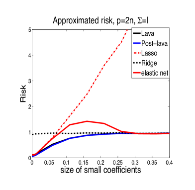
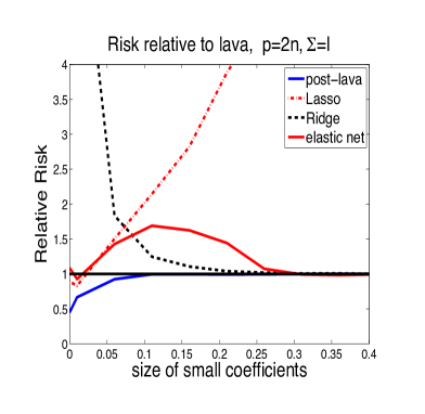
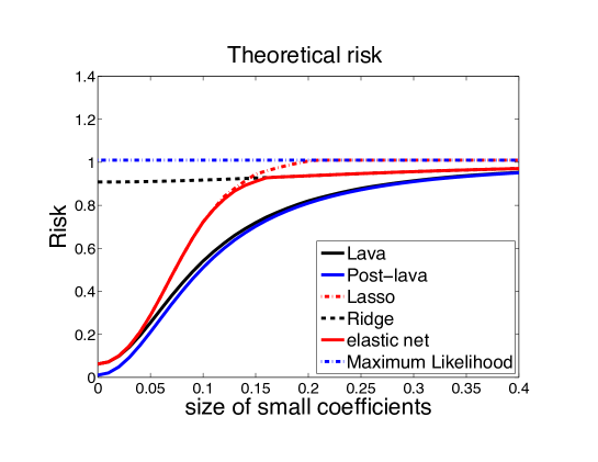
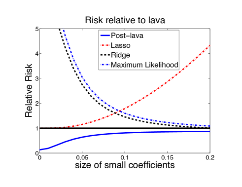
The lava estimator admits the lasso and ridge shrinkage methods as two extreme cases by respectively setting either λ2=subscript𝜆2\lambda_{2}=\infty or λ1=subscript𝜆1\lambda_{1}=\infty.111With λ1=subscript𝜆1\lambda_{1}=\infty or λ2=subscript𝜆2\lambda_{2}=\infty, we set λ1δ1=0subscript𝜆1subscriptnorm𝛿10\lambda_{1}\|\delta\|_{1}=0 when δ=0𝛿0\delta=0 or λ2β22=0subscript𝜆2superscriptsubscriptnorm𝛽220\lambda_{2}\|\beta\|_{2}^{2}=0 when β=0𝛽0\beta=0 so the problem is well-defined. In fact, it continuously connects the two shrinkage functions in a way that guarantees it will never produce a sparse solution when λ2<subscript𝜆2\lambda_{2}<\infty. Of course, sparsity is not a requirement for making good predictions. By construction, lava’s prediction risk is less than or equal to the prediction risk of the lasso and ridge methods with oracle choice of penalty levels for ridge, lasso, and lava; see Figure 1. Lava also tends to perform no worse than, and often performs significantly better than, ridge or lasso with penalty levels chosen by cross-validation; see Figures 4 and 5.

Note that our proposal is rather different from the elastic net method, which also uses a combination of 1subscript1\ell_{1} and 2subscript2\ell_{2} penalization. The elastic net penalty function is θλ2θ22+λ1θ1maps-to𝜃subscript𝜆2subscriptsuperscriptnorm𝜃22subscript𝜆1subscriptnorm𝜃1\theta\mapsto\lambda_{2}\|\theta\|^{2}_{2}+\lambda_{1}\|\theta\|_{1}, and thus the elastic net also includes lasso and ridge as extreme cases corresponding to λ2=0subscript𝜆20\lambda_{2}=0 and λ1=0subscript𝜆10\lambda_{1}=0 respectively. In sharp contrast to the lava method, the elastic net does not split θ𝜃\theta into a sparse and a dense part and will produce a sparse solution as long as λ1>0subscript𝜆10\lambda_{1}>0. Consequently, the elastic net method can be thought of as a sparsity-based method with additional shrinkage by ridge. The elastic net processes data very differently from lava (see Figure 2 below) and consequently has very different prediction risk behavior (see Figure 1 below).

We also consider the post-lava estimator which refits the sparse part of the model:

θ^post-lava=β^+δ~,subscript^𝜃post-lava^𝛽~𝛿\widehat{\theta}_{\mathrm{post}\text{-}\mathrm{lava}}=\widehat{\beta}+\widetilde{\delta}, (1.4)

where δ~~𝛿\widetilde{\delta} solves the following penalized optimization problem:

δ~=argminδp{(data,β^+δ):δj=0, if δ^j=0}.~𝛿subscript𝛿superscript𝑝:data^𝛽𝛿formulae-sequencesubscript𝛿𝑗0 if subscript^𝛿𝑗0\widetilde{\delta}=\arg\min_{\delta\in\mathbb{R}^{p}}\Big{\{}\ell(\mathrm{data},\widehat{\beta}+\delta):\delta_{j}=0,\text{ if }\widehat{\delta}_{j}=0\Big{\}}. (1.5)

This estimator removes the shrinkage bias induced by using the 1subscript1\ell_{1} penalty in estimation of the sparse part of the signal. Removing this bias sometimes results in further improvements of lava’s risk properties.
Refer to caption
Refer to caption
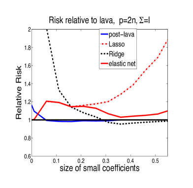
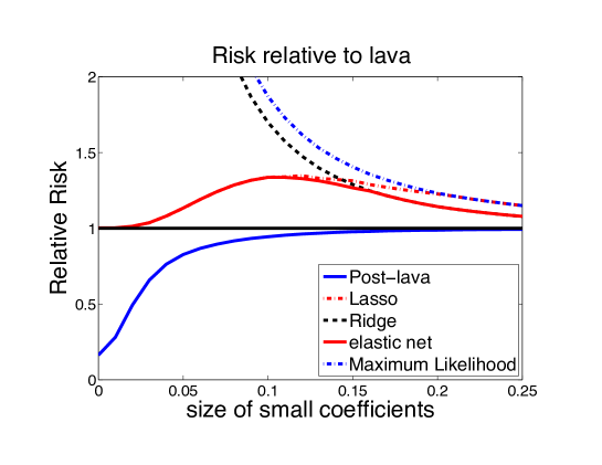
Figure 1. Exact risk and relative risk functions of lava, post-lava, ridge, lasso, elastic net, and maximum likelihood in the Gaussian sequence model with “sparse+dense” signal structure, using the oracle (risk minimizing) choices of penalty levels. See Section 2.5 for the description of the model. The size of “small coefficients” is shown on the horizontal axis. The size of these coefficients directly corresponds to the size of the “dense part” of the signal, with zero corresponding to the exactly sparse case. Relative risk plots the ratio of the risk of each estimator to the lava risk. Note that the relative risk plot is over a smaller set of sizes of small coefficients to accentuate comparisons over the region where there are the most interesting differences between the estimators.

We provide several theoretical and computational results about lava in this paper. First, we provide analytic expressions for the finite-sample risk function of the lava estimator as well as for other methods in the Gaussian sequence model and in a fixed design regression model with Gaussian errors. Within this context, we exhibit “sparse+dense” examples where lava significantly outperforms both lasso and ridge. Stein’s unbiased risk estimation plays a central role in our theoretical analysis, and we thus derive Stein’s unbiased risk estimator (SURE) for lava. We also characterize lava’s “Efron’s” degrees of freedom (Efron (2004)). Second, we give deviation bounds for the prediction risk of the lava estimator in regression models akin to those derived by Bickel et al. (2009) for lasso. Third, we illustrate lava’s performance relative to lasso, ridge, and elastic net through simulation experiments using penalty levels chosen via either minimizing the SURE or by k-fold cross-validation for all estimators. In our simulations, lava outperforms lasso and ridge in terms of prediction error over a wide range of regression models with coefficients that vary from having a rather sparse structure to having a very dense structure. When the model is very sparse, lava performs as well as lasso and outperforms ridge substantially. As the model becomes more dense in the sense of having the size of the “many small coefficients” increase, lava outperforms lasso and performs just as well as ridge. This is consistent with our theoretical results.

We conclude the introduction by noting that our proposed approach complements other recent approaches to structured sparsity problems such as those considered in fused sparsity estimation (Tibshirani et al. (2005) and Chen and Dalalyan (2012)) and structured matrix estimation problems (Candès et al. (2011), Chandrasekaran et al. (2011), Fan et al. (2013), and Klopp et al. (2014)). The latter line of research studied estimation of matrices that can be written as low rank plus sparse matrices. Our new results are related to but are sharply different from this latter line of work since our focus is on regression problems. Specifically, our chief objects of interest are regression coefficients along with the associated regression function and predictions of the outcome variable. Thus, the target statistical applications of our developed methods include prediction, classification, curve-fitting, and supervised learning. Another noteworthy point is that it is impossible to recover the “dense” and “sparse” components separately within our framework; instead, we recover the sum of the two components. By contrast, it is possible to recover the low-rank component of the matrix separately from the sparse part in some of the structured matrix estimation problems. This distinction serves to highlight the difference between structured matrix estimation problems and the framework discussed in this paper. Due to these differences, the mathematical side of our analysis needs to address a completely different set of issues than are addressed in the aforementioned structured matrix estimation problems.

We organize the rest of the paper as follows. Section 2 defines the lava shrinkage estimator in a canonical Gaussian sequence model, and derives its theoretical risk function. Section 3 defines and analyzes the lava estimator in the regression model. Section 4 provides computational examples, and Section 5 concludes. We give all proofs in the appendix.

Notation. The notation anbnless-than-or-similar-tosubscript𝑎𝑛subscript𝑏𝑛a_{n}\lesssim b_{n} means that anCbnsubscript𝑎𝑛𝐶subscript𝑏𝑛a_{n}\leq Cb_{n} for all n𝑛n, for some constant C𝐶C that does not depend on n𝑛n. The 2subscript2\ell_{2} and 1subscript1\ell_{1} norms are denoted by 2\|\cdot\|_{2} (or simply \|\cdot\|) and 1\|\cdot\|_{1}, respectively. The 0subscript0\ell_{0}-“norm”, 0\|\cdot\|_{0}, denotes the number of non-zero components of a vector, and the .\|.\|_{\infty} norm denotes a vector’s maximum absolute element. When applied to a matrix, \|\cdot\| denotes the operator norm. We use the notation ab=max(a,b)𝑎𝑏𝑎𝑏a\vee b=\max(a,b) and ab=min(a,b)𝑎𝑏𝑎𝑏a\wedge b=\min(a,b). We use xsuperscript𝑥x^{\prime} to denote the transpose of a column vector x𝑥x.

2. The lava estimator in a canonical model

2.1. The one dimensional case

Consider the simple problem where a scalar random variable is given by

Z=θ+ϵ,ϵN(0,σ2).formulae-sequence𝑍𝜃italic-ϵsimilar-toitalic-ϵ𝑁0superscript𝜎2Z=\theta+\epsilon,\quad\epsilon\sim N(0,\sigma^{2}).

We observe a realization z𝑧z of Z𝑍Z and wish to estimate θ𝜃\theta. Estimation will often involve the use of regularization or shrinkage via penalization to process input z𝑧z into output d(z)𝑑𝑧{d}(z), where the map zd(z)maps-to𝑧𝑑𝑧z\mapsto{d}(z) is commonly referred to as the shrinkage (or decision) function. A generic shrinkage estimator then takes the form θ^=d(Z)^𝜃𝑑𝑍\widehat{\theta}={d}(Z).

The commonly used lasso method uses 1subscript1\ell_{1}-penalization and gives rise to the lasso or soft-thresholding shrinkage function:

dlasso(z)=argminθ{(zθ)2+λl|θ|}=(|z|λl/2)+sign(z),subscript𝑑lasso𝑧subscript𝜃superscript𝑧𝜃2subscript𝜆𝑙𝜃subscript𝑧subscript𝜆𝑙2sign𝑧{d}_{\mathrm{lasso}}(z)=\ \arg\min_{\theta\in\mathbb{R}}\Big{\{}(z-\theta)^{2}+\lambda_{l}|\theta|\Big{\}}=(|z|-\lambda_{l}/2)_{+}\text{sign}(z),

where y+:=max(y,0)assignsubscript𝑦𝑦0y_{+}:=\max(y,0) and λl0subscript𝜆𝑙0\lambda_{l}\geq 0 is a penalty level. The use of the 2subscript2\ell_{2}-penalty in place of the 1subscript1\ell_{1} penalty yields the ridge shrinkage function:

dridge(z)=argminθ{(zθ)2+λr|θ|2}=z1+λr,subscript𝑑ridge𝑧subscript𝜃superscript𝑧𝜃2subscript𝜆𝑟superscript𝜃2𝑧1subscript𝜆𝑟{d}_{\mathrm{ridge}}(z)=\ \arg\min_{\theta\in\mathbb{R}}\ \Big{\{}(z-\theta)^{2}+\lambda_{r}|\theta|^{2}\Big{\}}=\frac{z}{1+\lambda_{r}},

where λr0subscript𝜆𝑟0\lambda_{r}\geq 0 is a penalty level. The lasso and ridge estimators then take the form

θ^lasso=dlasso(Z),θ^ridge=dridge(Z).formulae-sequencesubscript^𝜃lassosubscript𝑑lasso𝑍subscript^𝜃ridgesubscript𝑑ridge𝑍\widehat{\theta}_{\mathrm{lasso}}={d}_{\mathrm{lasso}}(Z),\quad\widehat{\theta}_{\mathrm{ridge}}={d}_{\mathrm{ridge}}(Z).

Other commonly used shrinkage methods include the elastic-net (Zou and Hastie (2005)), which uses θλ2|θ|2+λ1|θ|maps-to𝜃subscript𝜆2superscript𝜃2subscript𝜆1𝜃\theta\mapsto\lambda_{2}|\theta|^{2}+\lambda_{1}|\theta| as the penalty function; hard-thresholding; and the SCAD (Fan and Li (2001)), which uses a non-concave penalty function.

Motivated by points made in the introduction, we proceed differently. We decompose the signal into two components

θ=β+δ,𝜃𝛽𝛿\theta=\beta+\delta,

and use the different penalty functions – the 2subscript2\ell_{2} and 1subscript1\ell_{1} – for each component in order to predict θ𝜃\theta better. We thus consider the penalty function

(β,δ)λ2|β|2+λ1|δ|,maps-to𝛽𝛿subscript𝜆2superscript𝛽2subscript𝜆1𝛿(\beta,\delta)\mapsto\lambda_{2}|\beta|^{2}+\lambda_{1}|\delta|,

and introduce the “lava” shrinkage function zdlava(z)maps-to𝑧subscript𝑑lava𝑧z\mapsto{d}_{\mathrm{lava}}(z) defined by

dlava(z):=d2(z)+d1(z),assignsubscript𝑑lava𝑧subscript𝑑2𝑧subscript𝑑1𝑧\displaystyle{d}_{\mathrm{lava}}(z):={d}_{2}(z)+{d}_{1}(z),\quad (2.1)

where d1(z)subscript𝑑1𝑧{d}_{1}(z) and d2(z)subscript𝑑2𝑧{d}_{2}(z) solve the following penalized prediction problem:

(d2(z),d1(z)):=argmin(β,δ)2{[zβδ]2+λ2|β|2+λ1|δ|}.assignsubscript𝑑2𝑧subscript𝑑1𝑧subscript𝛽𝛿superscript2superscriptdelimited-[]𝑧𝛽𝛿2subscript𝜆2superscript𝛽2subscript𝜆1𝛿\displaystyle({d}_{2}(z),{d}_{1}(z)):=\arg\min_{(\beta,\delta)\in\mathbb{R}^{2}}\ \Big{\{}[z-\beta-\delta]^{2}+\lambda_{2}|\beta|^{2}+\lambda_{1}|\delta|\Big{\}}. (2.2)

Although the decomposition θ=β+δ𝜃𝛽𝛿\theta=\beta+\delta is not unique, the optimization problem (2.2) has a unique solution for any given (λ1,λ2)subscript𝜆1subscript𝜆2(\lambda_{1},\lambda_{2}). The proposal thus defines the lava estimator of θ𝜃\theta:

θ^lava=dlava(Z).subscript^𝜃lavasubscript𝑑lava𝑍\widehat{\theta}_{\mathrm{lava}}={d}_{\mathrm{lava}}(Z).

For large signals such that |z|>λ1/(2k)𝑧subscript𝜆12𝑘|z|>\lambda_{1}/(2k), lava has the same bias as the lasso. This bias can be removed through the use of the post-lava estimator

θ^postlava=dpostlava(Z),subscript^𝜃postlavasubscript𝑑postlava𝑍\widehat{\theta}_{\mathrm{post}-\mathrm{lava}}={d}_{\mathrm{post}-\mathrm{lava}}(Z),

where dpostlava(z):=d2(z)+d~1(z),assignsubscript𝑑postlava𝑧subscript𝑑2𝑧subscript~𝑑1𝑧{d}_{\mathrm{post}-\mathrm{lava}}(z):={d}_{2}(z)+\tilde{d}_{1}(z), and d~1(z)subscript~𝑑1𝑧\tilde{d}_{1}(z) solves the following penalized prediction problem:

d~1(z):=argminδ{[zd2(z)δ]2:δ=0 if d1(z)=0}.assignsubscript~𝑑1𝑧subscript𝛿:superscriptdelimited-[]𝑧subscript𝑑2𝑧𝛿2𝛿0 if subscript𝑑1𝑧0\displaystyle\tilde{d}_{1}(z):=\arg\min_{\delta\in\mathbb{R}}\Big{\{}[z-{d}_{2}(z)-\delta]^{2}:\delta=0\text{ if }{d}_{1}(z)=0\Big{\}}. (2.3)

The removal of this bias will result in improved risk performance relative to the original estimator in some contexts.

From the Karush-Kuhn-Tucker conditions, we obtain the explicit solution to (2.1).

Lemma 2.1.

For given penalty levels λ10subscript𝜆10\lambda_{1}\geq 0 and λ20subscript𝜆20\lambda_{2}\geq 0:

dlava(z)subscript𝑑lava𝑧\displaystyle{d}_{\mathrm{lava}}(z) =\displaystyle= (1k)z+k(|z|λ1/(2k))+sign(z)1𝑘𝑧𝑘subscript𝑧subscript𝜆12𝑘sign𝑧\displaystyle(1-k)z+k(|z|-\lambda_{1}/(2k))_{+}\mathrm{sign}(z) (2.4)
=\displaystyle= {zλ1/2,z>λ1/(2k)(1k)z,λ1/(2k)zλ1/(2k)z+λ1/2,z<λ1/(2k)cases𝑧subscript𝜆12𝑧subscript𝜆12𝑘missing-subexpression1𝑘𝑧subscript𝜆12𝑘𝑧subscript𝜆12𝑘missing-subexpression𝑧subscript𝜆12𝑧subscript𝜆12𝑘missing-subexpression\displaystyle\left\{\begin{array}[]{lll}z-\lambda_{1}/2,&z>\lambda_{1}/(2k)\\ (1-k)z,&-\lambda_{1}/(2k)\leq z\leq\lambda_{1}/(2k)\\ z+\lambda_{1}/2,&z<-\lambda_{1}/(2k)\end{array}\right. (2.8)

where k:=λ21+λ2.assign𝑘subscript𝜆21subscript𝜆2k:=\frac{\lambda_{2}}{1+\lambda_{2}}. The post-lava shrinkage function is given by

dpost-lava(z)={z,|z|>λ1/(2k),(1k)z,|z|λ1/(2k).subscript𝑑post-lava𝑧cases𝑧𝑧subscript𝜆12𝑘1𝑘𝑧𝑧subscript𝜆12𝑘{d}_{\mathrm{post}\text{-}\mathrm{lava}}(z)=\begin{cases}z,&|z|>\lambda_{1}/(2k),\\ (1-k)z,&|z|\leq\lambda_{1}/(2k).\end{cases}

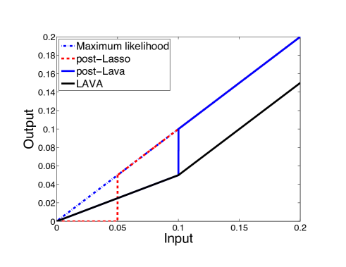
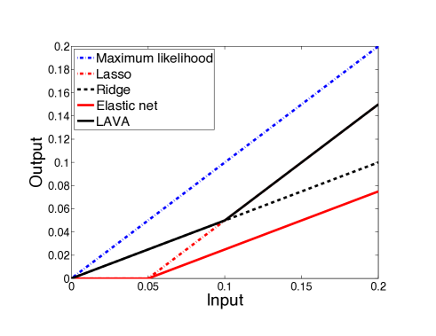
Figure 2 plots the lava shrinkage function along with various alternative shrinkage functions for z>0𝑧0z>0. The top panel of the figure compares lava shrinkage to ridge, lasso, and elastic net shrinkage. It is clear from the figure that lava shrinkage is different from lasso, ridge, and elastic net shrinkage. The figure also illustrates how lava provides a bridge between lasso and ridge, with the lava shrinkage function coinciding with the ridge shrinkage function for small values of the input z𝑧z and coinciding with the lasso shrinkage function for larger values of the input. Specifically, we see that the lava shrinkage function is a combination of lasso and ridge shrinkage that corresponds to using whichever of the lasso or ridge shrinkage is closer to the 45 degree line.

It is also useful to consider how lava and post-lava compare with the post-lasso or hard-thresholding shrinkage: dpost-lasso(z)=z1{|z|>λl/2}.subscript𝑑post-lasso𝑧𝑧1𝑧subscript𝜆𝑙2{d}_{\text{post-lasso}}(z)=z1\{|z|>\lambda_{l}/2\}. These different shrinkage functions are illustrated in the bottom panel of Figure 2.
Refer to caption
Refer to caption
Figure 2. Shrinkage functions. Here we plot shrinkage functions implied by lava and various commonly used penalized estimators. These shrinkage functions correspond to the case where penalty parameters are set as λ2=λr=1/2subscript𝜆2subscript𝜆𝑟12\lambda_{2}=\lambda_{r}=1/2 and λ1=λl=1/2subscript𝜆1subscript𝜆𝑙12\lambda_{1}=\lambda_{l}=1/2. In each figure, the light blue dashed line provides the 45 degree line coinciding to no shrinkage.

From (2.4), we observe some key characteristics of the lava shrinkage function:

1) The lava shrinkage admits the lasso and ridge shrinkages as two extreme cases. The lava and lasso shrinkage functions are the same when λ2=subscript𝜆2\lambda_{2}=\infty, and the ridge and lava shrinkage functions coincide if λ1=subscript𝜆1\lambda_{1}=\infty.

2) The lava shrinkage function dlava(z)subscript𝑑lava𝑧{d}_{\mathrm{lava}}(z) is a weighted average of data z𝑧z and the lasso shrinkage function dlasso(z)subscript𝑑lasso𝑧{d}_{\mathrm{lasso}}(z) with weights given by 1k1𝑘1-k and k𝑘k.

3) The lava never produces a sparse solution when λ2<subscript𝜆2\lambda_{2}<\infty: If λ2<subscript𝜆2\lambda_{2}<\infty, dlava(z)=0subscript𝑑lava𝑧0{d}_{\mathrm{lava}}(z)=0 if and only if z=0𝑧0z=0. This behavior is strongly different from elastic net which produces a sparse solution as long as λ1>0subscript𝜆10\lambda_{1}>0.

4) The lava shrinkage function continuously connects the ridge shrinkage function and the lasso shrinkage function. When |z|<λ1/(2k)𝑧subscript𝜆12𝑘|z|<\lambda_{1}/(2k), lava shrinkage is equal to ridge shrinkage; and when |z|>λ1/(2k)𝑧subscript𝜆12𝑘|z|>\lambda_{1}/(2k), lava shrinkage is equal to lasso shrinkage.

5) The lava shrinkage does exactly the opposite of the elastic net shrinkage. The elastic net shrinkage function coincides with the lasso shrinkage function when |z|<λ1/(2k)𝑧subscript𝜆12𝑘|z|<\lambda_{1}/(2k); and when |z|>λ1/(2k)𝑧subscript𝜆12𝑘|z|>\lambda_{1}/(2k), the elastic net shrinkage is the same as ridge shrinkage.

2.2. The risk function of the lava estimator in the one dimensional case

In the one-dimensional case with ZN(θ,σ2)similar-to𝑍𝑁𝜃superscript𝜎2Z\sim N(\theta,\sigma^{2}), a natural measure of the risk of a given estimator θ^=d(Z)^𝜃𝑑𝑍\widehat{\theta}={d}(Z) is given by

R(θ,θ^)𝑅𝜃^𝜃\displaystyle R(\theta,\widehat{\theta}) =\displaystyle= E[d(Z)θ]2Esuperscriptdelimited-[]𝑑𝑍𝜃2\displaystyle{\mathrm{E}}[{d}(Z)-\theta]^{2} (2.9)
=\displaystyle= σ2+E(Zd(Z))2+2E[(Zθ)d(Z)].superscript𝜎2Esuperscript𝑍𝑑𝑍22Edelimited-[]𝑍𝜃𝑑𝑍\displaystyle-\sigma^{2}+{\mathrm{E}}(Z-{d}(Z))^{2}+2{\mathrm{E}}[(Z-\theta){d}(Z)]. (2.10)

Let Pθ,σsubscriptP𝜃𝜎{\mathrm{P}}_{\theta,\sigma} denote the probability law of Z𝑍Z. Let ϕθ,σsubscriptitalic-ϕ𝜃𝜎\phi_{\theta,\sigma} be the density function of Z𝑍Z. We provide the risk functions of lava and post-lava in the following theorem. We also present the risk functions of ridge, elastic net, lasso, and post-lasso for comparison.

Theorem 2.1 (Risk Function of Lava and Related Estimators in the Scalar Case).

Suppose ZN(θ,σ2)similar-to𝑍𝑁𝜃superscript𝜎2Z\sim N(\theta,\sigma^{2}). Then for w=λ1/(2k)𝑤subscript𝜆12𝑘w=\lambda_{1}/(2k), k=λ2/(1+λ2)𝑘subscript𝜆21subscript𝜆2k=\lambda_{2}/(1+\lambda_{2}), h=1/(1+λ2)11subscript𝜆2h=1/(1+\lambda_{2}), d=λ1/(2(1+λ2))θ𝑑subscript𝜆121subscript𝜆2𝜃d=-\lambda_{1}/(2(1+\lambda_{2}))-\theta and g=λ1/(2(1+λ2))θ𝑔subscript𝜆121subscript𝜆2𝜃g=\lambda_{1}/(2(1+\lambda_{2}))-\theta, we have

R(θ,θ^lava)=k2(w+θ)ϕθ,σ(w)σ2+k2(θw)ϕθ,σ(w)σ2𝑅𝜃subscript^𝜃lavasuperscript𝑘2𝑤𝜃subscriptitalic-ϕ𝜃𝜎𝑤superscript𝜎2superscript𝑘2𝜃𝑤subscriptitalic-ϕ𝜃𝜎𝑤superscript𝜎2\displaystyle R(\theta,\widehat{\theta}_{\mathrm{lava}})=-k^{2}(w+\theta)\phi_{\theta,\sigma}(w)\sigma^{2}+k^{2}(\theta-w)\phi_{\theta,\sigma}(-w)\sigma^{2}
+(λ12/4+σ2)Pθ,σ(|Z|>w)+(θ2k2+(1k)2σ2)Pθ,σ(|Z|<w),superscriptsubscript𝜆124superscript𝜎2subscriptP𝜃𝜎𝑍𝑤superscript𝜃2superscript𝑘2superscript1𝑘2superscript𝜎2subscriptP𝜃𝜎𝑍𝑤\displaystyle\hskip 72.26999pt+(\lambda_{1}^{2}/4+\sigma^{2}){\mathrm{P}}_{\theta,\sigma}(|Z|>w)+(\theta^{2}k^{2}+(1-k)^{2}\sigma^{2}){\mathrm{P}}_{\theta,\sigma}(|Z|<w),
R(θ,θ^post-lava)=σ2[k2w+2kwk2θ]ϕθ,σ(w)+σ2[k2w+2kw+k2θ]ϕθ,σ(w)𝑅𝜃subscript^𝜃post-lavasuperscript𝜎2delimited-[]superscript𝑘2𝑤2𝑘𝑤superscript𝑘2𝜃subscriptitalic-ϕ𝜃𝜎𝑤superscript𝜎2delimited-[]superscript𝑘2𝑤2𝑘𝑤superscript𝑘2𝜃subscriptitalic-ϕ𝜃𝜎𝑤\displaystyle R(\theta,\widehat{\theta}_{\mathrm{post}\text{-}\mathrm{lava}})=\sigma^{2}[-k^{2}w+2kw-k^{2}\theta]\phi_{\theta,\sigma}(w)+\sigma^{2}[-k^{2}w+2kw+k^{2}\theta]\phi_{\theta,\sigma}(-w)
+σ2Pθ,σ(|Z|>w)+(k2θ2+(1k)2σ2)Pθ,σ(|Z|<w),superscript𝜎2subscriptP𝜃𝜎𝑍𝑤superscript𝑘2superscript𝜃2superscript1𝑘2superscript𝜎2subscriptP𝜃𝜎𝑍𝑤\displaystyle\hskip 72.26999pt+\sigma^{2}{\mathrm{P}}_{\theta,\sigma}(|Z|>w)+(k^{2}\theta^{2}+(1-k)^{2}\sigma^{2}){\mathrm{P}}_{\theta,\sigma}(|Z|<w),
R(θ,θ^lasso)=(λl/2+θ)ϕθ,σ(λl/2)σ2+(θλ1/2)ϕθ,σ(λl/2)σ2𝑅𝜃subscript^𝜃lassosubscript𝜆𝑙2𝜃subscriptitalic-ϕ𝜃𝜎subscript𝜆𝑙2superscript𝜎2𝜃subscript𝜆12subscriptitalic-ϕ𝜃𝜎subscript𝜆𝑙2superscript𝜎2\displaystyle R(\theta,\widehat{\theta}_{\mathrm{lasso}})=-(\lambda_{l}/2+\theta)\phi_{\theta,\sigma}(\lambda_{l}/2)\sigma^{2}+(\theta-\lambda_{1}/2)\phi_{\theta,\sigma}(-\lambda_{l}/2)\sigma^{2}
+(λl2/4+σ2)Pθ,σ(|Z|>λl/2)+θ2Pθ,σ(|Z|<λl/2),superscriptsubscript𝜆𝑙24superscript𝜎2subscriptP𝜃𝜎𝑍subscript𝜆𝑙2superscript𝜃2subscriptP𝜃𝜎𝑍subscript𝜆𝑙2\displaystyle\hskip 72.26999pt+(\lambda_{l}^{2}/4+\sigma^{2}){\mathrm{P}}_{\theta,\sigma}(|Z|>\lambda_{l}/2)+\theta^{2}{\mathrm{P}}_{\theta,\sigma}(|Z|<\lambda_{l}/2),
R(θ,θ^post-lasso)=(λl/2θ)ϕθ,σ(λl/2)σ2+(λl/2+θ)ϕθ,σ(λl/2)σ2𝑅𝜃subscript^𝜃post-lassosubscript𝜆𝑙2𝜃subscriptitalic-ϕ𝜃𝜎subscript𝜆𝑙2superscript𝜎2subscript𝜆𝑙2𝜃subscriptitalic-ϕ𝜃𝜎subscript𝜆𝑙2superscript𝜎2\displaystyle R(\theta,\widehat{\theta}_{\mathrm{post}\text{-}\mathrm{lasso}})=(\lambda_{l}/2-\theta)\phi_{\theta,\sigma}(\lambda_{l}/2)\sigma^{2}+(\lambda_{l}/2+\theta)\phi_{\theta,\sigma}(-\lambda_{l}/2)\sigma^{2}
+σ2Pθ,σ(|Z|>λr/2)+θ2Pθ,σ(|Z|<λr/2),superscript𝜎2subscriptP𝜃𝜎𝑍subscript𝜆𝑟2superscript𝜃2subscriptP𝜃𝜎𝑍subscript𝜆𝑟2\displaystyle\hskip 72.26999pt+\sigma^{2}{\mathrm{P}}_{\theta,\sigma}(|Z|>\lambda_{r}/2)+\theta^{2}{\mathrm{P}}_{\theta,\sigma}(|Z|<\lambda_{r}/2),
R(θ,θ^ridge)=θ2k~2+(1k~)2σ2,k~=λr/(1+λr),formulae-sequence𝑅𝜃subscript^𝜃ridgesuperscript𝜃2superscript~𝑘2superscript1~𝑘2superscript𝜎2~𝑘subscript𝜆𝑟1subscript𝜆𝑟\displaystyle R(\theta,\widehat{\theta}_{\mathrm{ridge}})=\theta^{2}\widetilde{k}^{2}+(1-\widetilde{k})^{2}\sigma^{2},\quad\widetilde{k}=\lambda_{r}/(1+\lambda_{r}),
R(θ,θ^elasticnet)=σ2(h2λ1/2+h2θ+2dh)ϕθ,σ(λ1/2)𝑅𝜃subscript^𝜃elasticnetsuperscript𝜎2superscript2subscript𝜆12superscript2𝜃2𝑑subscriptitalic-ϕ𝜃𝜎subscript𝜆12\displaystyle R(\theta,\widehat{\theta}_{\mathrm{elastic\ net}})=\sigma^{2}(h^{2}\lambda_{1}/2+h^{2}\theta+2dh)\phi_{\theta,\sigma}(\lambda_{1}/2)
σ2(h2λ1/2+h2θ+2gh)ϕθ,σ(λ1/2)+θ2Pθ,σ(|Z|<λ1/2)superscript𝜎2superscript2subscript𝜆12superscript2𝜃2𝑔subscriptitalic-ϕ𝜃𝜎subscript𝜆12superscript𝜃2subscriptP𝜃𝜎𝑍subscript𝜆12\displaystyle\hskip 72.26999pt-\sigma^{2}(-h^{2}\lambda_{1}/2+h^{2}\theta+2gh)\phi_{\theta,\sigma}(-\lambda_{1}/2)+\theta^{2}{\mathrm{P}}_{\theta,\sigma}(|Z|<\lambda_{1}/2)
+((hθ+d)2+h2σ2)Pθ,σ(Z>λ1/2)superscript𝜃𝑑2superscript2superscript𝜎2subscriptP𝜃𝜎𝑍subscript𝜆12\displaystyle\hskip 72.26999pt+((h\theta+d)^{2}+h^{2}\sigma^{2}){\mathrm{P}}_{\theta,\sigma}(Z>\lambda_{1}/2)
+((hθ+g)2+h2σ2)Pθ,σ(Z<λ1/2).superscript𝜃𝑔2superscript2superscript𝜎2subscriptP𝜃𝜎𝑍subscript𝜆12\displaystyle\hskip 72.26999pt+((h\theta+g)^{2}+h^{2}\sigma^{2}){\mathrm{P}}_{\theta,\sigma}(Z<-\lambda_{1}/2).

These results for the one-dimensional case provide a key building block for results in the multidimensional case provided below. In particular, we build from these results to show that the lava estimator performs very favorably relative to, and can substantially dominate, the maximum likelihood estimator, the ridge estimator, and 1subscript1\ell_{1}-based estimators (such as lasso and elastic-net) in interesting multidimensional settings.

2.3. Multidimensional case

We consider now the canonical Gaussian model or the Gaussian sequence model. In this case, we have that

ZNp(θ,σ2Ip)similar-to𝑍subscript𝑁𝑝𝜃superscript𝜎2subscript𝐼𝑝Z\sim N_{p}(\theta,\sigma^{2}I_{p})

is a single observation from a multivariate normal distribution where θ=(θ1,,θp)𝜃superscriptsubscript𝜃1subscript𝜃𝑝\theta=(\theta_{1},...,\theta_{p})^{\prime} is a p𝑝p-dimensional vector. A fundamental result for this model is that the maximum likelihood estimator Z𝑍Z is inadmissible and can be dominated by the ridge estimator and related shrinkage procedures when p3𝑝3p\geq 3 (e.g. Stein (1956)).

In this model, the lava estimator is given by

θ^lava:=(θ^lava,1,,θ^lava,p):=(dlava(Z1),,dlava(Zp)),assignsubscript^𝜃lavasuperscriptsubscript^𝜃lava1subscript^𝜃lava𝑝assignsuperscriptsubscript𝑑lavasubscript𝑍1subscript𝑑lavasubscript𝑍𝑝\widehat{\theta}_{\text{lava}}:=(\widehat{\theta}_{\mathrm{lava},1},...,\widehat{\theta}_{\mathrm{lava},p})^{\prime}:=({d}_{\text{lava}}(Z_{1}),...,{d}_{\text{lava}}(Z_{p}))^{\prime},

where dlava(z)subscript𝑑lava𝑧{d}_{\text{lava}}(z) is the lava shrinkage function as in (2.8). The estimator is designed to capture the case where

θ=βdense part+δsparse part𝜃subscript𝛽dense partsubscript𝛿sparse part\theta=\underbrace{\beta}_{\text{dense part}}+\underbrace{\delta}_{\text{sparse part}}

is formed by combining a sparse vector δ𝛿\delta that has a relatively small number of non-zero entries which are all large in magnitude and a dense vector β𝛽\beta that may contain very many small non-zero entries. This model for θ𝜃\theta is “sparse+dense.” It includes cases that are not well-approximated by “sparse” models - models in which a very small number of parameters are large and the rest are zero - or by “dense” models - models in which very many coefficients are non-zero but all coefficients are of similar magnitude. This structure thus includes cases that pose challenges for estimators such as the lasso and elastic net that are designed for sparse models and for estimators such as ridge that are designed for dense models.

Remark 2.1.

The regression model with Gaussian noise and an orthonormal design is a special case of the multidimensional canonical model. Consider

Y=Xθ+U,UXN(0,σu2In),formulae-sequence𝑌𝑋𝜃𝑈similar-toconditional𝑈𝑋𝑁0superscriptsubscript𝜎𝑢2subscript𝐼𝑛Y=X\theta+U,\quad U\mid X\sim N(0,\sigma_{u}^{2}I_{n}),

where Y𝑌Y and U𝑈U are n×1𝑛1n\times 1 random vectors and X𝑋X is an n×p𝑛𝑝n\times p random or fixed matrix, with n𝑛n and p𝑝p respectively denoting the sample size and the dimension of θ𝜃\theta. Suppose 1nXX=Ip1𝑛superscript𝑋𝑋subscript𝐼𝑝\frac{1}{n}X^{\prime}X=I_{p} a.s.. with pn𝑝𝑛p\leq n. Then we have the canonical multidimensional model:

Z=θ+ϵ,Z=1nXY,ϵ=1nXUN(0,σ2Ip),σ2=σu2n.Z=\theta+\epsilon,\ \ Z=\frac{1}{n}X^{\prime}Y,\quad\epsilon=\frac{1}{n}X^{\prime}U\sim N(0,\sigma^{2}I_{p}),\quad\sigma^{2}=\frac{\sigma^{2}_{u}}{n}.\quad\scriptstyle\blacksquare

All of the shrinkage estimators discussed in Section 2.1 generalize to the multidimensional case in the same way as lava. Let zde(z)maps-to𝑧subscript𝑑𝑒𝑧z\mapsto{d}_{e}(z) be the shrinkage function associated with estimator e𝑒e in the one dimensional setting where e𝑒e can take values in the set

={lava,post-lava,ridge,lasso,post-lasso,elasticnet}.lavapost-lavaridgelassopost-lassoelasticnet\mathcal{E}=\{\mathrm{lava},\mathrm{post\text{-}lava},\mathrm{ridge},\mathrm{lasso},\mathrm{post\text{-}lasso},\mathrm{elastic\ net}\}.

We then have a similar estimator in the multidimensional case given by

θ^e:=(θ^e,1,,θ^e,p):=(de(Z1),,de(Zp)).assignsubscript^𝜃𝑒superscriptsubscript^𝜃𝑒1subscript^𝜃𝑒𝑝assignsuperscriptsubscript𝑑𝑒subscript𝑍1subscript𝑑𝑒subscript𝑍𝑝\widehat{\theta}_{e}:=(\widehat{\theta}_{e,1},...,\widehat{\theta}_{e,p})^{\prime}:=({d}_{e}(Z_{1}),...,{d}_{e}(Z_{p}))^{\prime}.

The risk calculation from the one dimensional case then caries over to the multidimensional case since

R(θ,θ^e):=Eθθ^e22=j=1pR(θj,θ^e,j).assignR𝜃subscript^𝜃𝑒Esuperscriptsubscriptnorm𝜃subscript^𝜃𝑒22superscriptsubscript𝑗1𝑝𝑅subscript𝜃𝑗subscript^𝜃𝑒𝑗\mathrm{R}(\theta,\widehat{\theta}_{e}):={\mathrm{E}}\|\theta-\widehat{\theta}_{e}\|_{2}^{2}=\sum_{j=1}^{p}R(\theta_{j},\widehat{\theta}_{e,j}).

Given this fact, we immediately obtain the following result.

Theorem 2.2 (Risk Function of Lava and Related Estimators in the Multi-Dimensional Case).

If ZN(0,σ2Ip)similar-to𝑍𝑁0superscript𝜎2subscript𝐼𝑝Z\sim N(0,\sigma^{2}I_{p}), then for any e𝑒e\in\mathcal{E} we have that

R(θ,θ^e)=j=1pR(θj,θ^e,j),R𝜃subscript^𝜃𝑒superscriptsubscript𝑗1𝑝𝑅subscript𝜃𝑗subscript^𝜃𝑒𝑗\mathrm{R}(\theta,\widehat{\theta}_{e})=\sum_{j=1}^{p}R(\theta_{j},\widehat{\theta}_{e,j}),

where R(,)𝑅R(\cdot,\cdot) is the uni-dimensional risk function characterized in Theorem 2.1.

These risk functions are illustrated in Figure 1 in a prototypical “sparse+dense” model generated according to the model discussed in detail in Section 2.5. The tuning parameters used in this figure are the best possible (risk minimizing or oracle) choices of the penalty levels found by minimizing the risk expression given in Theorem 2.2.

2.4. Canonical plug-in choice of penalty levels

We now discuss simple, rule-of-thumb choices for the penalty levels for lasso (λlsubscript𝜆𝑙\lambda_{l}), ridge (λrsubscript𝜆𝑟\lambda_{r}) and lava (λ1,λ2subscript𝜆1subscript𝜆2\lambda_{1},\lambda_{2}). In the Gaussian model, a canonical choice of λlsubscript𝜆𝑙\lambda_{l} is

λl=2σΦ1(1c/(2p)),subscript𝜆𝑙2𝜎superscriptΦ11𝑐2𝑝\lambda_{l}=2\sigma{\Phi^{-1}(1-c/(2p))},

which satisfies

P(maxjp|Zjθj|λl/2)1c;Psubscript𝑗𝑝subscript𝑍𝑗subscript𝜃𝑗subscript𝜆𝑙21𝑐{\mathrm{P}}\left(\max_{j\leq p}|Z_{j}-\theta_{j}|\leq\lambda_{l}/2\right)\geq 1-c;

see, e.g., Donoho and Johnstone (1995). Here Φ()Φ\Phi(\cdot) denotes the standard normal cumulative distribution function, and c𝑐c is a pre-determined significance level which is often set to 0.05. The risk function for ridge is simple, and an analytic solution to the risk minimizing choice of ridge tuning parameter is given by

λr=σ2(p/θ22).subscript𝜆𝑟superscript𝜎2𝑝superscriptsubscriptnorm𝜃22\lambda_{r}=\sigma^{2}(p/\|\theta\|_{2}^{2}).

As for the tuning parameters for lava, recall that the lava estimator in the Gaussian model is

θ^lavasubscript^𝜃lava\displaystyle\widehat{\theta}_{\text{lava}} =\displaystyle= (θ^lava,1,,θ^lava,p),θ^lava,j=β^j+δ^j,j=1,,p,formulae-sequencesuperscriptsubscript^𝜃lava1subscript^𝜃lava𝑝subscript^𝜃lava𝑗subscript^𝛽𝑗subscript^𝛿𝑗𝑗1𝑝\displaystyle(\widehat{\theta}_{\mathrm{lava},1},...,\widehat{\theta}_{\mathrm{lava},p})^{\prime},\quad\widehat{\theta}_{\mathrm{lava},j}=\widehat{\beta}_{j}+\widehat{\delta}_{j},\quad j=1,...,p,
(β^j,δ^j)subscript^𝛽𝑗subscript^𝛿𝑗\displaystyle(\widehat{\beta}_{j},\widehat{\delta}_{j}) =\displaystyle= argmin(βj,δj)2(Zjβjδj)2+λ2|βj|2+λ1|δj|.\displaystyle\arg\min_{(\beta_{j},\delta_{j})\in\mathbb{R}^{2}}(Z_{j}-\beta_{j}-\delta_{j})^{2}+\lambda_{2}|\beta_{j}|^{2}+\lambda_{1}|\delta_{j}|.

If the dense component β𝛽\beta were known, then following Donoho and Johnstone (1995) would suggest setting

λ1=2σΦ1(1c/(2p))subscript𝜆12𝜎superscriptΦ11𝑐2𝑝\lambda_{1}=2\sigma{\Phi^{-1}(1-c/(2p))}

as a canonical choice of λ1subscript𝜆1\lambda_{1} for estimating δ𝛿\delta. If the sparse component δ𝛿\delta were known, one could adopt

λ2=σ2(p/β22)subscript𝜆2superscript𝜎2𝑝superscriptsubscriptnorm𝛽22\lambda_{2}=\sigma^{2}(p/\|\beta\|_{2}^{2})

as a choice of λ2subscript𝜆2\lambda_{2} for estimating β𝛽\beta following the logic for the standard ridge estimator.

We refer to these choices as the “canonical plug-in” tuning parameters and use them in constructing the risk comparisons in the following subsection. We note that the lasso choice is motivated by a sparse model and does not naturally adapt to or make use of the true structure of θ𝜃\theta. The ridge penalty choice is explicitly tied to risk minimization and relies on using knowledge of the true θ𝜃\theta. The lava choices for the parameters on the 1subscript1\ell_{1} and 2subscript2\ell_{2} penalties are, as noted immediately above, motivated by the respective choices in lasso and ridge. As such, the motivations and feasibility of these canonical choices are not identical across methods, and the risk comparisons in the following subsection should be interpreted within this light.

2.5. Some risk comparisons in a canonical Gaussian model

To compare the risk functions of lava, lasso, and ridge estimators, we consider a canonical Gaussian model, where

θ1=3,θj=0.1q,j=2,,p,formulae-sequencesubscript𝜃13formulae-sequencesubscript𝜃𝑗0.1𝑞𝑗2𝑝\theta_{1}=3,\quad\theta_{j}=0.1q,\quad j=2,...,p,

for some q0𝑞0q\geq 0. We set the noise level to be σ2=0.12superscript𝜎2superscript0.12\sigma^{2}=0.1^{2}. The parameter θ𝜃\theta can be decomposed as θ=β+δ𝜃𝛽𝛿\theta=\beta+\delta, where the sparse component is δ=(3,0,,0)𝛿superscript300\delta=(3,0,...,0)^{\prime}, and the dense component is

β=(0,0.1q,,0.1q),𝛽superscript00.1𝑞0.1𝑞\beta=(0,0.1q,...,0.1q)^{\prime},

where q𝑞q describes the “size of small coefficients.” The canonical tuning parameters are λl=λ1=2σΦ1(1c/(2p))subscript𝜆𝑙subscript𝜆12𝜎superscriptΦ11𝑐2𝑝\lambda_{l}=\lambda_{1}=2\sigma{\Phi^{-1}(1-c/(2p))}, λr=σ2p/(3+0.12q2(p1))subscript𝜆𝑟superscript𝜎2𝑝3superscript0.12superscript𝑞2𝑝1\lambda_{r}=\sigma^{2}p/(3+0.1^{2}q^{2}(p-1)) and λ2=σ2p/(0.12q2(p1))subscript𝜆2superscript𝜎2𝑝superscript0.12superscript𝑞2𝑝1\lambda_{2}=\sigma^{2}p/(0.1^{2}q^{2}(p-1)).

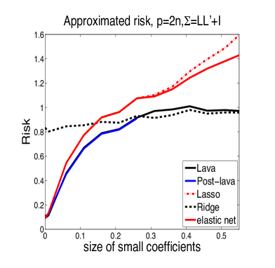
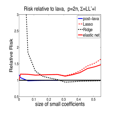
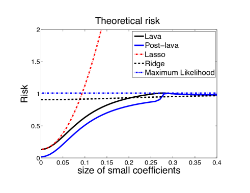
Figure 1 (given in the introduction) compares risks of lava, lasso, ridge, elastic net, and the maximum likelihood estimators as functions of the size of the small coefficients q𝑞q, using the ideal (risk minimizing or oracle choices) of the penalty levels. Figure 3 compares risks of lava, lasso, ridge and the maximum likelihood estimators using the “canonical plug-in” penalty levels discussed above. Theoretical risks are plotted as a function of the size of the small coefficients q𝑞q. We see from these figures that regardless of how we choose the penalty levels – ideally or via the plug-in rules – lava strictly dominates the competing methods in this “sparse+dense” model. Compared to lasso, the proposed lava estimator does about as well as lasso when the signal is sparse and does significantly better than lasso when the signal is non-sparse. Compared to ridge, the lava estimator does about as well as ridge when the signal is dense and does significantly better than ridge when the signal is sparse.
Refer to caption
Refer to caption
Figure 3. Exact risk functions of lava, post-lava, ridge, lasso, and maximum likelihood in the Gaussian sequence model with “sparse+dense” signal structure, using the canonical “plug-in” choices of penalty levels. See Section 2.5 for the description of penalty levels and the model. The size of “small coefficients” is shown on the horizontal axis. The size of these coefficients directly corresponds to the size of the “dense part” of the signal, with zero corresponding to the exactly sparse case. Relative risk plots the ratio of the risk of each estimator to the lava risk, R(θ,θ^e)/R(θ,θ^lava)R𝜃subscript^𝜃𝑒R𝜃subscript^𝜃lava\mathrm{R}(\theta,\widehat{\theta}_{e})/\mathrm{R}(\theta,\widehat{\theta}_{\mathrm{lava}}). Note that the relative risk plot is over a smaller set of sizes to accentuate comparisons over the region where there are the most interesting differences between the estimators.

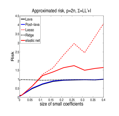
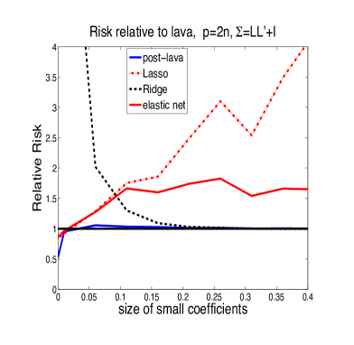
In Section 5 we further explore the use of feasible, data-driven choices of penalty levels via cross-validation and SURE minimization; see Figures 4 and 5. We do so in the context of the Gaussian regression model with fixed regressors. With either cross-validation or SURE minmization, the ranking of the estimators remains unchanged, with lava consistently dominating lasso, ridge, and the elastic net.

Stein (1956) proved that a ridge estimator strictly dominates maximum likelihood in the Gaussian sequence model once p3𝑝3p\geq 3. In the comparisons above, we also see that the lava estimator strictly dominates the maximum likelihood estimator; and one wonders whether this domination has a theoretical underpinning similar to Stein’s result for ridge. The following result provides some (partial) support for this phenomenon for the lava estimator with the plug-in penalty levels. The result shows that, for a sufficiently large n𝑛n and p𝑝p, lava does indeed uniformly dominate the maximum likelihood estimator on the compact set {θ=β+δ:β+δ<M}conditional-set𝜃𝛽𝛿subscriptnorm𝛽subscriptnorm𝛿𝑀\{\theta=\beta+\delta:\|\beta\|_{\infty}+\|\delta\|_{\infty}<M\}.

Lemma 2.2 (Relative Risk of Lava vs. Maximum Likelihood ).

Suppose ZNp(θ,σ2Ip)similar-to𝑍subscript𝑁𝑝𝜃superscript𝜎2subscript𝐼𝑝Z\sim N_{p}(\theta,\sigma^{2}I_{p}), where θ𝜃\theta can be decomposed into θ=β+δ𝜃𝛽𝛿\theta=\beta+\delta with s=j=1p1{δj0}<p𝑠superscriptsubscript𝑗1𝑝1subscript𝛿𝑗0𝑝s=\sum_{j=1}^{p}1\{\delta_{j}\neq 0\}<p. Let λ1subscript𝜆1\lambda_{1} and λ2subscript𝜆2\lambda_{2} be chosen with the plug-in rule given in Section 2.4. Then uniformly for θ{θ=β+δ:β+δ<M}𝜃conditional-set𝜃𝛽𝛿subscriptnorm𝛽subscriptnorm𝛿𝑀\theta\in\{\theta=\beta+\delta:\|\beta\|_{\infty}+\|\delta\|_{\infty}<M\}, when σlogp>2M+33σ𝜎𝑝2𝑀33𝜎\sigma\sqrt{\log p}>2M+33\sigma, M2logp>16σ2superscript𝑀2𝑝16superscript𝜎2M^{2}\log p>16\sigma^{2}, and πc2logp1𝜋superscript𝑐2𝑝1\pi c^{2}{\log p}\geq 1, we have

RR:=Eθ^lava(Z)θ22EZθ22β22σ2p+β22+3sM2pσ2+42πp1/16(1+7Mσp1/16).assign𝑅𝑅Esuperscriptsubscriptnormsubscript^𝜃lava𝑍𝜃22Esuperscriptsubscriptnorm𝑍𝜃22superscriptsubscriptnorm𝛽22superscript𝜎2𝑝superscriptsubscriptnorm𝛽223𝑠superscript𝑀2𝑝superscript𝜎242𝜋superscript𝑝11617𝑀𝜎superscript𝑝116RR:=\frac{{\mathrm{E}}\|\widehat{\theta}_{\mathrm{lava}}(Z)-\theta\|_{2}^{2}}{{\mathrm{E}}\|Z-\theta\|_{2}^{2}}\leq\frac{\|\beta\|_{2}^{2}}{\sigma^{2}p+\|\beta\|_{2}^{2}}+\frac{3sM^{2}}{p\sigma^{2}}+\frac{4}{\sqrt{2\pi}p^{1/16}}\left(1+\frac{7M}{\sigma p^{1/16}}\right).
Remark 2.2.

Note that

Rd2=β22σ2p+β22subscriptsuperscript𝑅2𝑑superscriptsubscriptnorm𝛽22superscript𝜎2𝑝superscriptsubscriptnorm𝛽22R^{2}_{d}=\frac{\|\beta\|_{2}^{2}}{\sigma^{2}p+\|\beta\|_{2}^{2}}

measures the proportion of the total variation of Zδ𝑍𝛿Z-\delta around 00 that is explained by the dense part of the signal. If Rd2subscriptsuperscript𝑅2𝑑R^{2}_{d} is bounded away from 111 and M𝑀M and σ2>0superscript𝜎20\sigma^{2}>0 are fixed, then the risk of lava becomes uniformly smaller than the risk of the maximum likelihood estimator on a compact parameter space as p𝑝p\to\infty and s/p0𝑠𝑝0s/p\to 0. Indeed, if Rd2subscriptsuperscript𝑅2𝑑R^{2}_{d} is bounded away from 111, then

3sM2pσ2+42πp1/16(1+7Mσp1/16)0RR=Rd2+o(1)<1.3𝑠superscript𝑀2𝑝superscript𝜎242𝜋superscript𝑝11617𝑀𝜎superscript𝑝1160𝑅𝑅subscriptsuperscript𝑅2𝑑𝑜11\frac{3sM^{2}}{p\sigma^{2}}+\frac{4}{\sqrt{2\pi}p^{1/16}}\left(1+\frac{7M}{\sigma p^{1/16}}\right)\to 0\implies RR=R^{2}_{d}+o(1)<1.

Moreover, we have RR0𝑅𝑅0RR\to 0 if Rd20subscriptsuperscript𝑅2𝑑0R^{2}_{d}\to 0. That is, the lava estimator becomes infinitely more asymptotically efficient than the maximum likelihood estimator in terms of relative risk. \blacksquare

2.6. Stein’s unbiased risk estimation for lava

Stein (1981) proposed a useful risk estimate based on the integration by parts formula, now commonly referred to as Stein’s unbiased risk estimate (SURE). This subsection derives SURE for the lava shrinkage in the multivariate Gaussian model.

Note that

Eθ^lavaθ22=pσ2+EZθ^lava22+2E[(Zθ)θ^lava].Esuperscriptsubscriptnormsubscript^𝜃lava𝜃22𝑝superscript𝜎2Esuperscriptsubscriptnorm𝑍subscript^𝜃lava222Edelimited-[]superscript𝑍𝜃subscript^𝜃lava{\mathrm{E}}\|\widehat{\theta}_{\text{lava}}-\theta\|_{2}^{2}=-p\sigma^{2}+{\mathrm{E}}\|Z-\widehat{\theta}_{\text{lava}}\|_{2}^{2}+2{\mathrm{E}}[(Z-\theta)^{\prime}\widehat{\theta}_{\text{lava}}]. (2.11)

An essential component to understanding the risk is given by applying Stein’s formula to calculate E[(Zθ)θ^lava]Edelimited-[]superscript𝑍𝜃subscript^𝜃lava{\mathrm{E}}[(Z-\theta)^{\prime}\widehat{\theta}_{\text{lava}}]. A closed-form expression for this expression in the one-dimensional case is given in equation (A.15) in the appendix. The following result provides the SURE for lava in the more general multidimensional case.

Theorem 2.3 (SURE for lava).

Suppose Z=(Z1,,Zp)Np(θ,σ2Ip)𝑍superscriptsubscript𝑍1subscript𝑍𝑝similar-tosubscript𝑁𝑝𝜃superscript𝜎2subscript𝐼𝑝Z=(Z_{1},...,Z_{p})^{\prime}\sim N_{p}(\theta,\sigma^{2}I_{p}). Then

E[(Zθ)θ^lava]=p(1k)σ2+kσ2j=1pPθj,σ(|Zj|>λ1/(2k)).Edelimited-[]superscript𝑍𝜃subscript^𝜃lava𝑝1𝑘superscript𝜎2𝑘superscript𝜎2superscriptsubscript𝑗1𝑝subscriptPsubscript𝜃𝑗𝜎subscript𝑍𝑗subscript𝜆12𝑘{\mathrm{E}}[(Z-\theta)^{\prime}\widehat{\theta}_{\mathrm{lava}}]=p(1-k)\sigma^{2}+k\sigma^{2}\sum_{j=1}^{p}{\mathrm{P}}_{\theta_{j},\sigma}(|Z_{j}|>\lambda_{1}/(2k)).

In addition, let {Zij}i=1nsuperscriptsubscriptsubscript𝑍𝑖𝑗𝑖1𝑛\{Z_{ij}\}_{i=1}^{n} be identically distributed as Zjsubscript𝑍𝑗Z_{j} for each j𝑗j. Then

R^(θ,θ^lava)=(12k)pσ2+1ni=1nZidlava(Zi)22+2kσ21ni=1nj=1p1{|Zij|>λ1/(2k)}.^R𝜃subscript^𝜃lava12𝑘𝑝superscript𝜎21𝑛superscriptsubscript𝑖1𝑛superscriptsubscriptnormsubscript𝑍𝑖subscript𝑑lavasubscript𝑍𝑖222𝑘superscript𝜎21𝑛superscriptsubscript𝑖1𝑛superscriptsubscript𝑗1𝑝1subscript𝑍𝑖𝑗subscript𝜆12𝑘\widehat{\mathrm{R}}(\theta,\widehat{\theta}_{\mathrm{lava}})=(1-2k)p\sigma^{2}+\frac{1}{n}\sum_{i=1}^{n}\|Z_{i}-{d}_{\mathrm{lava}}(Z_{i})\|_{2}^{2}+2k\sigma^{2}\frac{1}{n}\sum_{i=1}^{n}\sum_{j=1}^{p}1\{|Z_{ij}|>\lambda_{1}/(2k)\}.

is an unbiased estimator of R(θ,θ^lava)R𝜃subscript^𝜃lava\mathrm{R}(\theta,\widehat{\theta}_{\mathrm{lava}}).

3. Lava in the Regression Model

3.1. Definition of Lava in the Regression Model

Consider a fixed design regression model:

Y=Xθ0+U,UN(0,σu2In),formulae-sequence𝑌𝑋subscript𝜃0𝑈similar-to𝑈𝑁0superscriptsubscript𝜎𝑢2subscript𝐼𝑛Y=X\theta_{0}+U,\quad U\sim N(0,\sigma_{u}^{2}I_{n}),

where Y=(y1,,yn)𝑌superscriptsubscript𝑦1subscript𝑦𝑛Y=(y_{1},...,y_{n})^{\prime}, X=(X1,,Xn)𝑋superscriptsubscript𝑋1subscript𝑋𝑛X=(X_{1},...,X_{n})^{\prime}, and θ0subscript𝜃0\theta_{0} is the true regression coefficient. Following the previous discussion, we assume that

θ0=β0+δ0subscript𝜃0subscript𝛽0subscript𝛿0\theta_{0}=\beta_{0}+\delta_{0}

is “sparse+dense” with sparse component δ0subscript𝛿0\delta_{0} and dense component β0subscript𝛽0\beta_{0}. Again, this coefficient structure includes cases which cannot be well-approximated by traditional sparse models or traditional dense models and will pose challenges for estimation strategies tailored to sparse settings, such as lasso and similar methods, or strategies tailored to dense settings, such as ridge.

In order to define the estimator we shall rely on the normalization condition that

n1[XX]jj=1,j=1,,p.formulae-sequencesuperscript𝑛1subscriptdelimited-[]superscript𝑋𝑋𝑗𝑗1𝑗1𝑝n^{-1}[X^{\prime}X]_{jj}=1,\quad j=1,...,p. (3.1)

Note that without this normalization, the penalty terms below would have to be modified in order to insure equivariance of the estimator to changes of scale in the columns of X𝑋X.

The lava estimator θ^lavasubscript^𝜃lava\widehat{\theta}_{\mathrm{lava}} of θ0subscript𝜃0\theta_{0} solves the following optimization problem:

θ^lavasubscript^𝜃lava\displaystyle\widehat{\theta}_{\text{lava}} :=assign\displaystyle:= β^+δ^,^𝛽^𝛿\displaystyle\widehat{\beta}+\widehat{\delta}, (3.2)
(β^,δ^)^𝛽^𝛿\displaystyle(\widehat{\beta},\widehat{\delta}) :=assign\displaystyle:= argmin(β,δ)2p{1nYX(β+δ)22+λ2β22+λ1δ1}.subscriptsuperscriptsuperscript𝛽superscript𝛿superscript2𝑝1𝑛superscriptsubscriptnorm𝑌𝑋𝛽𝛿22subscript𝜆2superscriptsubscriptnorm𝛽22subscript𝜆1subscriptnorm𝛿1\displaystyle\arg\min_{(\beta^{\prime},\delta^{\prime})^{\prime}\in\mathbb{R}^{2p}}\left\{\frac{1}{n}\|Y-X(\beta+\delta)\|_{2}^{2}+\lambda_{2}\|\beta\|_{2}^{2}+\lambda_{1}\|\delta\|_{1}\right\}. (3.3)

The lava program splits parameter θ𝜃\theta into the sum of β𝛽\beta and δ𝛿\delta and penalizes these two parts using the 2subscript2\ell_{2} and 1subscript1\ell_{1} penalties. Thus, the 1subscript1\ell_{1}- penalization regularizes the estimator of the sparse part δ0subscript𝛿0\delta_{0} of θ0subscript𝜃0\theta_{0} and produces a sparse solution δ^^𝛿\widehat{\delta}. The 2subscript2\ell_{2}-penalization regularizes the estimator of the dense part β0subscript𝛽0\beta_{0} of θ0subscript𝜃0\theta_{0} and produces a dense solution β^^𝛽\widehat{\beta}. The resulting estimator of θ0subscript𝜃0\theta_{0} is then simply the sum of the sparse estimator δ^^𝛿\widehat{\delta} and the dense estimator β^^𝛽\widehat{\beta}.

3.2. A Key Profile Characterization and Some Insights.

The lava estimator can be computed in the following way. For a fixed δ𝛿\delta, we minimize

β^(δ)=argminβp{1nYX(β+δ)22+λ2β22},^𝛽𝛿subscript𝛽superscript𝑝1𝑛superscriptsubscriptnorm𝑌𝑋𝛽𝛿22subscript𝜆2superscriptsubscriptnorm𝛽22\widehat{\beta}(\delta)=\arg\min_{\beta\in\mathbb{R}^{p}}\left\{\frac{1}{n}\|Y-X(\beta+\delta)\|_{2}^{2}+\lambda_{2}\|\beta\|_{2}^{2}\right\},

with respect to β𝛽\beta. This program is simply the well-known ridge regression problem, and the solution is

β^(δ)=(XX+nλ2Ip)1X(YXδ).^𝛽𝛿superscriptsuperscript𝑋𝑋𝑛subscript𝜆2subscript𝐼𝑝1superscript𝑋𝑌𝑋𝛿\widehat{\beta}(\delta)=(X^{\prime}X+n\lambda_{2}I_{p})^{-1}X^{\prime}(Y-X\delta).

By substituting β=β^(δ)𝛽^𝛽𝛿\beta=\widehat{\beta}(\delta) into the objective function, we then define an 1subscript1\ell_{1}-penalized quadratic program which we can solve for δ^^𝛿\widehat{\delta}:

δ^=argminδp{1nYX(β^(δ)+δ)22+λ2β^(δ)22+λ1δ1}.^𝛿subscript𝛿superscript𝑝1𝑛superscriptsubscriptnorm𝑌𝑋^𝛽𝛿𝛿22subscript𝜆2superscriptsubscriptnorm^𝛽𝛿22subscript𝜆1subscriptnorm𝛿1\widehat{\delta}=\arg\min_{\delta\in\mathbb{R}^{p}}\left\{\frac{1}{n}\|Y-X(\widehat{\beta}(\delta)+\delta)\|_{2}^{2}+\lambda_{2}\|\widehat{\beta}(\delta)\|_{2}^{2}+\lambda_{1}\|\delta\|_{1}\right\}. (3.4)

The lava solution is then given by θ^=β^(δ^)+δ^^𝜃^𝛽^𝛿^𝛿\widehat{\theta}=\widehat{\beta}(\widehat{\delta})+\widehat{\delta}. The following result provides a useful characterization of the solution.

Theorem 3.1 (A Key Characterization of the Profiled Lava Program).

Define ridge-projection matrices,

𝖯λ2=X(XX+nλ2Ip)1Xand𝖪λ2=In𝖯λ2,subscript𝖯subscript𝜆2𝑋superscriptsuperscript𝑋𝑋𝑛subscript𝜆2subscript𝐼𝑝1superscript𝑋𝑎𝑛𝑑subscript𝖪subscript𝜆2subscript𝐼𝑛subscript𝖯subscript𝜆2\operatorname{\mathsf{P}}_{\lambda_{2}}=X(X^{\prime}X+n\lambda_{2}I_{p})^{-1}X^{\prime}\ and\ \operatorname{\mathsf{K}}_{\lambda_{2}}=I_{n}-\operatorname{\mathsf{P}}_{\lambda_{2}},

and transformed data,

Y~=𝖪λ21/2YandX~=𝖪λ21/2X.~𝑌superscriptsubscript𝖪subscript𝜆212𝑌𝑎𝑛𝑑~𝑋superscriptsubscript𝖪subscript𝜆212𝑋\widetilde{Y}=\operatorname{\mathsf{K}}_{\lambda_{2}}^{1/2}Y\ and\ \widetilde{X}=\operatorname{\mathsf{K}}_{\lambda_{2}}^{1/2}X.

Then

δ^=argminδp{1nY~X~δ22+λ1δ1}^𝛿subscript𝛿superscript𝑝1𝑛superscriptsubscriptnorm~𝑌~𝑋𝛿22subscript𝜆1subscriptnorm𝛿1\widehat{\delta}=\arg\min_{\delta\in\mathbb{R}^{p}}\left\{\frac{1}{n}\|\widetilde{Y}-\widetilde{X}\delta\|_{2}^{2}+\lambda_{1}\|\delta\|_{1}\right\} (3.5)

and

Xθ^lava=𝖯λ2Y+𝖪λ2Xδ^.𝑋subscript^𝜃lavasubscript𝖯subscript𝜆2𝑌subscript𝖪subscript𝜆2𝑋^𝛿X\widehat{\theta}_{\mathrm{lava}}=\operatorname{\mathsf{P}}_{\lambda_{2}}Y+\operatorname{\mathsf{K}}_{\lambda_{2}}X\widehat{\delta}. (3.6)

The theorem shows that solving for the sparse part δ^^𝛿\widehat{\delta} of the lava estimator is equivalent to solving for the parameter in a standard lasso problem using transformed data. This result is key to both computation and our theoretical analysis of the estimator.

Remark 3.1 (Insights derived from Theorem 3.1).

Suppose δ0subscript𝛿0\delta_{0} were known. Let W=YXδ0𝑊𝑌𝑋subscript𝛿0W=Y-X\delta_{0} be the response vector after removing the sparse signal, and note that we equivalently have W=Xβ0+U𝑊𝑋subscript𝛽0𝑈W=X\beta_{0}+U. A natural estimator for β0subscript𝛽0\beta_{0} in this setting is then the ridge estimator of W𝑊W on X𝑋X:

β^(δ0)=(XX+nλ2Ip)1XW.^𝛽subscript𝛿0superscriptsuperscript𝑋𝑋𝑛subscript𝜆2subscript𝐼𝑝1superscript𝑋𝑊\widehat{\beta}(\delta_{0})=(X^{\prime}X+n\lambda_{2}I_{p})^{-1}X^{\prime}W.

Denote the prediction error based on this ridge estimator as

Dridge(λ2)=Xβ^(δ0)Xβ0=𝖪λ2Xβ0+𝖯λ2U.subscriptDridgesubscript𝜆2𝑋^𝛽subscript𝛿0𝑋subscript𝛽0subscript𝖪subscript𝜆2𝑋subscript𝛽0subscript𝖯subscript𝜆2𝑈\textsf{D}_{\text{ridge}}(\lambda_{2})=X\widehat{\beta}(\delta_{0})-X\beta_{0}=-\operatorname{\mathsf{K}}_{\lambda_{2}}X\beta_{0}+\operatorname{\mathsf{P}}_{\lambda_{2}}U.

Under mild regularity conditions on β0subscript𝛽0\beta_{0} and the design matrix, Hsu et al. (2014) showed that

1nDridge(λ2)2=oP(1).1𝑛superscriptnormsubscriptDridgesubscript𝜆22subscript𝑜𝑃1\frac{1}{n}\|\textsf{D}_{\text{ridge}}(\lambda_{2})\|^{2}=o_{P}(1).

Using Theorem 3.1, the prediction error of lava can be written as

Xθ^lavaXθ0=𝖯λ2Y+𝖪λ2Xδ^Xβ0Xδ0=Dridge(λ2)+𝖪λ2X(δ^δ0).𝑋subscript^𝜃lava𝑋subscript𝜃0subscript𝖯subscript𝜆2𝑌subscript𝖪subscript𝜆2𝑋^𝛿𝑋subscript𝛽0𝑋subscript𝛿0subscriptDridgesubscript𝜆2subscript𝖪subscript𝜆2𝑋^𝛿subscript𝛿0X\widehat{\theta}_{\text{lava}}-X\theta_{0}=\operatorname{\mathsf{P}}_{\lambda_{2}}Y+\operatorname{\mathsf{K}}_{\lambda_{2}}X\widehat{\delta}-X\beta_{0}-X\delta_{0}=\textsf{D}_{\text{ridge}}(\lambda_{2})+\operatorname{\mathsf{K}}_{\lambda_{2}}X(\widehat{\delta}-\delta_{0}). (3.7)

Hence, lava has vanishing prediction error as long as

1n𝖪λ2X(δ^δ0)22=oP(1).1𝑛superscriptsubscriptnormsubscript𝖪subscript𝜆2𝑋^𝛿subscript𝛿022subscript𝑜𝑃1\frac{1}{n}\|\operatorname{\mathsf{K}}_{\lambda_{2}}X(\widehat{\delta}-\delta_{0})\|_{2}^{2}=o_{P}(1). (3.8)

Condition (3.8) is related to the performance of the lasso in the transformed problem (3.5). Examination of (3.5) shows that it corresponds to a sparse regression model with approximation errors 𝖪λ21/2Xβ0superscriptsubscript𝖪subscript𝜆212𝑋subscript𝛽0\operatorname{\mathsf{K}}_{\lambda_{2}}^{1/2}X\beta_{0}: For U~=𝖪λ21/2U~𝑈superscriptsubscript𝖪subscript𝜆212𝑈\widetilde{U}=\operatorname{\mathsf{K}}_{\lambda_{2}}^{1/2}U,

Y~=X~δ0+U~+𝖪λ21/2Xβ0.~𝑌~𝑋subscript𝛿0~𝑈superscriptsubscript𝖪subscript𝜆212𝑋subscript𝛽0\widetilde{Y}=\widetilde{X}\delta_{0}+\widetilde{U}+\operatorname{\mathsf{K}}_{\lambda_{2}}^{1/2}X\beta_{0}. (3.9)

Under conditions such as those given in Hsu et al. (2014), the approximation error obeys

1n𝖪λ21/2Xβ022=oP(1).1𝑛superscriptsubscriptnormsuperscriptsubscript𝖪subscript𝜆212𝑋subscript𝛽022subscript𝑜𝑃1\frac{1}{n}\|\operatorname{\mathsf{K}}_{\lambda_{2}}^{1/2}X\beta_{0}\|_{2}^{2}=o_{P}(1). (3.10)

It is also known that the lasso estimator performs well in sparse models with vanishing approximation errors. The lasso estimator attains rates of convergence in the prediction norm that are the sum of the usual rate of convergence in the case without approximation errors and the rate at which the approximation error vanishes; see, e.g., Belloni and Chernozhukov (2013). Thus, we anticipate that (3.8) will hold.

To help understand the plausibility of condition (3.10), consider an orthogonal design where 1nXX=Ip1𝑛superscript𝑋𝑋subscript𝐼𝑝\frac{1}{n}X^{\prime}X=I_{p}. In this case, it is straightforward to verify that 𝖪λ21/2=𝖪λ2superscriptsubscript𝖪subscript𝜆212subscript𝖪superscriptsubscript𝜆2\operatorname{\mathsf{K}}_{\lambda_{2}}^{1/2}=\operatorname{\mathsf{K}}_{\lambda_{2}^{*}} where λ2=λ2/(1+λ2λ2).superscriptsubscript𝜆2subscript𝜆21subscript𝜆2subscript𝜆2\lambda_{2}^{*}=\sqrt{\lambda_{2}}/(\sqrt{1+\lambda_{2}}-\sqrt{\lambda_{2}}). Hence, X~β0=𝖪λ2Xβ0~𝑋subscript𝛽0subscript𝖪superscriptsubscript𝜆2𝑋subscript𝛽0\widetilde{X}\beta_{0}=\operatorname{\mathsf{K}}_{\lambda_{2}^{*}}X\beta_{0} is a component of the prediction bias from a ridge estimator with tuning parameter λ2superscriptsubscript𝜆2\lambda_{2}^{*} and is stochastically negligible. We present the rigorous asymptotic analysis for the general case in Section 3.5. \blacksquare

3.3. Degrees of Freedom and SURE

Degrees of freedom is often used to quantify model complexity and to construct adaptive model selection criteria for selecting tuning parameters. In a Gaussian linear regression model YN(Xθ0,σu2In)similar-to𝑌𝑁𝑋subscript𝜃0superscriptsubscript𝜎𝑢2subscript𝐼𝑛Y\sim N(X\theta_{0},\sigma_{u}^{2}I_{n}) with a fixed design, we can define the degrees of freedom of the mean fit Xθ^𝑋^𝜃X\widehat{\theta} to be

df(θ^)=1σu2E[(YXθ0)Xθ^];df^𝜃1superscriptsubscript𝜎𝑢2Edelimited-[]superscript𝑌𝑋subscript𝜃0𝑋^𝜃\mathrm{df}(\widehat{\theta})=\frac{1}{\sigma_{u}^{2}}{\mathrm{E}}[(Y-X\theta_{0})^{\prime}X\widehat{\theta}];

see, e.g., Efron (2004). Note that this quantity is also an important component of the mean squared prediction risk:

E1nXθ^Xθ022=σu2+E1nXθ^Y22+2σu2ndf(θ^).E1𝑛superscriptsubscriptnorm𝑋^𝜃𝑋subscript𝜃022superscriptsubscript𝜎𝑢2E1𝑛superscriptsubscriptnorm𝑋^𝜃𝑌222superscriptsubscript𝜎𝑢2𝑛df^𝜃{\mathrm{E}}\frac{1}{n}\|X\widehat{\theta}-X\theta_{0}\|_{2}^{2}=-\sigma_{u}^{2}+{\mathrm{E}}\frac{1}{n}\|X\widehat{\theta}-Y\|_{2}^{2}+\frac{2\sigma_{u}^{2}}{n}\mathrm{df}(\widehat{\theta}).

Stein (1981)’s SURE theory provides a tractable way of deriving an unbiased estimator of the degrees of freedom, and thus the mean squared prediction risk. Specifically, write θ^=d(Y,X)^𝜃𝑑𝑌𝑋\widehat{\theta}=d(Y,X) as a function of Y𝑌Y, conditional on X𝑋X. Suppose d(,X):np:𝑑𝑋superscript𝑛superscript𝑝d(\cdot,X):\mathbb{R}^{n}\to\mathbb{R}^{p} is almost differentiable; see Meyer and Woodroofe (2000) and Efron et al. (2004)). For f:nn:𝑓superscript𝑛superscript𝑛f:\mathbb{R}^{n}\to\mathbb{R}^{n} differentiable at y𝑦y, define

yf(y):=[fij(y)],(i,j){1,,n}2,fij(y):=yjfi(y),formulae-sequenceassignsubscript𝑦𝑓𝑦delimited-[]subscript𝑓𝑖𝑗𝑦formulae-sequence𝑖𝑗superscript1𝑛2assignsubscript𝑓𝑖𝑗𝑦subscript𝑦𝑗subscript𝑓𝑖𝑦\partial_{y}f(y):=[\partial f_{ij}(y)],\quad(i,j)\in\{1,...,n\}^{2},\quad\partial f_{ij}(y):=\frac{\partial}{\partial y_{j}}f_{i}(y),
yf(y):=tr(yf(y)).assignsubscript𝑦𝑓𝑦trsubscript𝑦𝑓𝑦\nabla_{y}\cdot f(y):=\text{tr}(\partial_{y}f(y)).

Let Xisuperscriptsubscript𝑋𝑖X_{i}^{\prime} denote the i𝑖i-th row of X𝑋X, i=1,,n𝑖1𝑛i=1,...,n. Then, from Stein (1981), we have that

1σu2E[(YXθ0)Xd(Y,X)]=E[y(Xd(Y,X))]=tr(y[Xd(Y,X)]).1superscriptsubscript𝜎𝑢2Edelimited-[]superscript𝑌𝑋subscript𝜃0𝑋𝑑𝑌𝑋Edelimited-[]subscript𝑦𝑋𝑑𝑌𝑋trsubscript𝑦delimited-[]𝑋𝑑𝑌𝑋\frac{1}{\sigma_{u}^{2}}{\mathrm{E}}[(Y-X\theta_{0})^{\prime}Xd(Y,X)]={\mathrm{E}}[\nabla_{y}\cdot(Xd(Y,X))]=\text{tr}\big{(}\partial_{y}[Xd(Y,X)]\big{)}.

An unbiased estimator of the term on the right-hand-side of the display may then be constructed using its sample analog.

In this subsection, we derive the degrees of freedom of the lava, and thus a SURE of its mean squared prediction risk. By Theorem 3.1,

y(Xdlava(y,X))subscript𝑦𝑋subscript𝑑lava𝑦𝑋\displaystyle\nabla_{y}\cdot(Xd_{\text{lava}}(y,X)) =\displaystyle= tr(𝖯λ2)+y(𝖪λ2Xdlasso(𝖪λ21/2y,𝖪λ21/2X))trsubscript𝖯subscript𝜆2subscript𝑦subscript𝖪subscript𝜆2𝑋subscript𝑑lassosuperscriptsubscript𝖪subscript𝜆212𝑦superscriptsubscript𝖪subscript𝜆212𝑋\displaystyle\text{tr}(\operatorname{\mathsf{P}}_{\lambda_{2}})+\nabla_{y}\cdot(\operatorname{\mathsf{K}}_{\lambda_{2}}Xd_{\mathrm{lasso}}(\operatorname{\mathsf{K}}_{\lambda_{2}}^{1/2}y,\operatorname{\mathsf{K}}_{\lambda_{2}}^{1/2}X)) (3.11)
=\displaystyle= tr(𝖯λ2)+tr(𝖪λ2y[Xdlasso(𝖪λ21/2y,X~)]),trsubscript𝖯subscript𝜆2trsubscript𝖪subscript𝜆2subscript𝑦delimited-[]𝑋subscript𝑑lassosuperscriptsubscript𝖪subscript𝜆212𝑦~𝑋\displaystyle\text{tr}(\operatorname{\mathsf{P}}_{\lambda_{2}})+\text{tr}\left(\operatorname{\mathsf{K}}_{\lambda_{2}}\partial_{y}[Xd_{\mathrm{lasso}}(\operatorname{\mathsf{K}}_{\lambda_{2}}^{1/2}y,\widetilde{X})]\right), (3.12)

where dlava(y,X)subscript𝑑lava𝑦𝑋d_{\mathrm{lava}}(y,X) is the lava estimator on the data (y,X)𝑦𝑋(y,X) and dlasso(𝖪λ21/2y,𝖪λ21/2X))d_{\mathrm{lasso}}(\operatorname{\mathsf{K}}_{\lambda_{2}}^{1/2}y,\operatorname{\mathsf{K}}_{\lambda_{2}}^{1/2}X)) is the lasso estimator on the data (𝖪λ21/2y,𝖪λ21/2X)superscriptsubscript𝖪subscript𝜆212𝑦superscriptsubscript𝖪subscript𝜆212𝑋(\operatorname{\mathsf{K}}_{\lambda_{2}}^{1/2}y,\operatorname{\mathsf{K}}_{\lambda_{2}}^{1/2}X) with the penalty level λ1subscript𝜆1\lambda_{1}. The almost differentiability of the map ydlasso(𝖪λ21/2y,𝖪λ21/2X)maps-to𝑦subscript𝑑lassosuperscriptsubscript𝖪subscript𝜆212𝑦superscriptsubscript𝖪subscript𝜆212𝑋y\mapsto d_{\mathrm{lasso}}(\operatorname{\mathsf{K}}_{\lambda_{2}}^{1/2}y,\operatorname{\mathsf{K}}_{\lambda_{2}}^{1/2}X) follows from the almost differentiability of the map udlasso(u,𝖪λ21/2X)maps-to𝑢subscript𝑑lasso𝑢superscriptsubscript𝖪subscript𝜆212𝑋u\mapsto d_{\mathrm{lasso}}(u,\operatorname{\mathsf{K}}_{\lambda_{2}}^{1/2}X), which holds by the results in Dossal et al. (2011) and Tibshirani and Taylor (2012).

The following theorem presents the degrees of freedom and SURE for lava. Let J^={jp:δ^j0}^𝐽conditional-set𝑗𝑝subscript^𝛿𝑗0\widehat{J}=\{j\leq p:\widehat{\delta}_{j}\neq 0\} be the active set of the sparse component estimator with cardinality denoted by |J^|^𝐽|\widehat{J}|. Recall that X~=𝖪λ21/2X~𝑋superscriptsubscript𝖪subscript𝜆212𝑋\widetilde{X}=\operatorname{\mathsf{K}}_{\lambda_{2}}^{1/2}X. Let X~J^subscript~𝑋^𝐽\widetilde{X}_{\hat{J}} be an n×|J^|𝑛^𝐽n\times|\widehat{J}| submatrix of X~~𝑋\widetilde{X} whose columns are those corresponding to the entries in J^^𝐽\widehat{J}. Let Asuperscript𝐴A^{-} denote the Moore-Penrose pseudo-inverse of a square matrix A𝐴A.

Theorem 3.2 (SURE for Lava in Regression).

Suppose YN(Xθ0,σu2In)similar-to𝑌𝑁𝑋subscript𝜃0superscriptsubscript𝜎𝑢2subscript𝐼𝑛Y\sim N(X\theta_{0},\sigma_{u}^{2}I_{n}). Let

𝖪~J^=IX~J^(X~J^X~J^)X~J^subscript~𝖪^𝐽𝐼subscript~𝑋^𝐽superscriptsuperscriptsubscript~𝑋^𝐽subscript~𝑋^𝐽superscriptsubscript~𝑋^𝐽\widetilde{\operatorname{\mathsf{K}}}_{\hat{J}}=I-\widetilde{X}_{\hat{J}}(\widetilde{X}_{\hat{J}}^{\prime}\widetilde{X}_{\hat{J}})^{-}\widetilde{X}_{\hat{J}}^{\prime}

be the projection matrix onto the unselected columns of the transformed variables. We have that

df(θ^lava)=E[rank(X~J^)+tr(𝖪~J^𝖯λ2)].dfsubscript^𝜃lavaEdelimited-[]ranksubscript~𝑋^𝐽trsubscript~𝖪^𝐽subscript𝖯subscript𝜆2\mathrm{df}(\widehat{\theta}_{\mathrm{lava}})={\mathrm{E}}[\operatorname{rank}(\widetilde{X}_{\hat{J}})+\operatorname{tr}(\widetilde{\operatorname{\mathsf{K}}}_{\hat{J}}\operatorname{\mathsf{P}}_{\lambda_{2}})].

Therefore, the SURE of E1nXθ^lavaXθ022E1𝑛superscriptsubscriptnorm𝑋subscript^𝜃lava𝑋subscript𝜃022{\mathrm{E}}\frac{1}{n}\|X\widehat{\theta}_{\mathrm{lava}}-X\theta_{0}\|_{2}^{2} is given by

σu2+1nXθ^lavaY22+2σu2nrank(X~J^)+2σu2ntr(𝖪~J^𝖯λ2).superscriptsubscript𝜎𝑢21𝑛superscriptsubscriptnorm𝑋subscript^𝜃lava𝑌222superscriptsubscript𝜎𝑢2𝑛ranksubscript~𝑋^𝐽2superscriptsubscript𝜎𝑢2𝑛trsubscript~𝖪^𝐽subscript𝖯subscript𝜆2-\sigma_{u}^{2}+\frac{1}{n}\|X\widehat{\theta}_{\mathrm{lava}}-Y\|_{2}^{2}+\frac{2\sigma_{u}^{2}}{n}\operatorname{rank}(\widetilde{X}_{\hat{J}})+\frac{2\sigma_{u}^{2}}{n}\operatorname{tr}(\widetilde{\operatorname{\mathsf{K}}}_{\hat{J}}\operatorname{\mathsf{P}}_{\lambda_{2}}).

3.4. Post-lava in regression

We can also remove the shrinkage bias in the sparse component introduced by the 1subscript1\ell_{1}-penalization via a post-selection procedure. Specifically, let (β^,δ^^𝛽^𝛿\widehat{\beta},\widehat{\delta}) respectively denote the lava estimator of the dense and sparse components. Define the post-lava estimator as follows:

θ^post-lavasubscript^𝜃post-lava\displaystyle\widehat{\theta}_{\text{post-lava}} =\displaystyle= β^+δ~,^𝛽~𝛿\displaystyle\widehat{\beta}+\widetilde{\delta},
δ~~𝛿\displaystyle\widetilde{\delta} =\displaystyle= argminδp{1nYXβ^Xδ22:δj=0 if δ^j=0}.\displaystyle\arg\min_{\delta\in\mathbb{R}^{p}}\left\{\frac{1}{n}\|Y-X\widehat{\beta}-X\delta\|_{2}^{2}:\quad\delta_{j}=0\text{ if }\widehat{\delta}_{j}=0\right\}.

Let XJ^subscript𝑋^𝐽X_{\hat{J}} be an n×|J^|𝑛^𝐽n\times|\widehat{J}| submatrix of X𝑋X whose columns are selected by J^^𝐽\widehat{J}. Then we can partition δ~=(δ~J^,0)~𝛿superscriptsubscript~𝛿^𝐽0\widetilde{\delta}=(\widetilde{\delta}_{\hat{J}},0)^{\prime}, where δ~J^=(XJ^XJ^)XJ^(YXβ^)subscript~𝛿^𝐽superscriptsuperscriptsubscript𝑋^𝐽subscript𝑋^𝐽superscriptsubscript𝑋^𝐽𝑌𝑋^𝛽\widetilde{\delta}_{\hat{J}}=(X_{\hat{J}}^{\prime}X_{\hat{J}})^{-}X_{\hat{J}}^{\prime}(Y-X\widehat{\beta}). Write 𝖯J^=XJ^(XJ^XJ^)XJ^subscript𝖯^𝐽subscript𝑋^𝐽superscriptsuperscriptsubscript𝑋^𝐽subscript𝑋^𝐽superscriptsubscript𝑋^𝐽\operatorname{\mathsf{P}}_{\hat{J}}=X_{\hat{J}}(X_{\hat{J}}^{\prime}X_{\hat{J}})^{-}X_{\hat{J}}^{\prime} and 𝖪J^=In𝖯J^subscript𝖪^𝐽subscript𝐼𝑛subscript𝖯^𝐽\operatorname{\mathsf{K}}_{\hat{J}}=I_{n}-\operatorname{\mathsf{P}}_{\hat{J}}. The post-lava prediction for Xθ𝑋𝜃X\theta is:

Xθ^post-lava=𝖯J^Y+𝖪J^Xβ^.𝑋subscript^𝜃post-lavasubscript𝖯^𝐽𝑌subscript𝖪^𝐽𝑋^𝛽X\widehat{\theta}_{\text{post-lava}}=\operatorname{\mathsf{P}}_{\hat{J}}Y+\operatorname{\mathsf{K}}_{\hat{J}}X\widehat{\beta}.

In addition, note that the lava estimator satisfies Xβ^=𝖯λ2(YXδ^)𝑋^𝛽subscript𝖯subscript𝜆2𝑌𝑋^𝛿X\widehat{\beta}=\operatorname{\mathsf{P}}_{\lambda_{2}}(Y-X\widehat{\delta}). We then have the following expression of Xθ^post-lava𝑋subscript^𝜃post-lavaX\widehat{\theta}_{\text{post-lava}}.

Lemma 3.1.

Let U^:=YXθ^lavaassign^𝑈𝑌𝑋subscript^𝜃lava\widehat{U}:=Y-X\widehat{\theta}_{\mathrm{lava}}. Then Xθ^post-lava=Xθ^lava+𝖯J^U^.𝑋subscript^𝜃post-lava𝑋subscript^𝜃lavasubscript𝖯^𝐽^𝑈X\widehat{\theta}_{\mathrm{post}\text{-}\mathrm{lava}}=X\widehat{\theta}_{\mathrm{lava}}+\operatorname{\mathsf{P}}_{\hat{J}}\widehat{U}.

The above lemma reveals that the post-lava corrects the 1subscript1\ell_{1}-shrinkage bias of the original lava fit by adding the projection of the lava residual onto the subspace of the selected regressors. This correction is in the same spirit as the post-lasso correction for shrinkage bias in the standard lasso problem; see Belloni and Chernozhukov (2013).

Remark 3.2.

We note that the SURE for post-lava may not exist, though an estimate of the upper bound of the risk function may be available, because of the impossibility results for constructing unbiased estimators for non-differentiable functions; see Hirano and Porter (2012). \blacksquare

3.5. Deviation Bounds for Prediction Errors

In the following, we develop deviation bounds for the lava prediction error: 1nXθ^lavaXθ0221𝑛superscriptsubscriptnorm𝑋subscript^𝜃lava𝑋subscript𝜃022\frac{1}{n}\|X\widehat{\theta}_{\text{lava}}-X\theta_{0}\|_{2}^{2}. We continue to work with the decomposition θ0=β0+δ0subscript𝜃0subscript𝛽0subscript𝛿0\theta_{0}=\beta_{0}+\delta_{0} and will show that lava performs well in terms of rates on the prediction error in this setting. According to the discussion in Section 3.2, there are three sources of prediction error: (i) Dridge(λ2)subscriptDridgesubscript𝜆2\textsf{D}_{\text{ridge}}(\lambda_{2}), (ii) X~β0~𝑋subscript𝛽0\widetilde{X}\beta_{0} and (iii) 𝖪λ2X(δ^δ0)subscript𝖪subscript𝜆2𝑋^𝛿subscript𝛿0\operatorname{\mathsf{K}}_{\lambda_{2}}X(\widehat{\delta}-\delta_{0}). The behavior of the first two terms is determined by the behavior of the ridge estimator of the dense component β0subscript𝛽0\beta_{0}, and the behavior of the third term is determined by the behavior of the lasso estimator on the transformed data.

We assume that UN(0,σu2In)similar-to𝑈𝑁0superscriptsubscript𝜎𝑢2subscript𝐼𝑛U\sim N(0,\sigma_{u}^{2}I_{n}) and that X𝑋X is fixed. As in the lasso analysis of Bickel et al. (2009), a key quantity is the maximal norm of the score:

Λ=2nX~U~=2nX𝖪λ2U.Λsubscriptnorm2𝑛superscript~𝑋~𝑈subscriptnorm2𝑛superscript𝑋subscript𝖪subscript𝜆2𝑈\Lambda=\left\|\frac{2}{n}\widetilde{X}^{\prime}\widetilde{U}\right\|_{\infty}=\left\|\frac{2}{n}X^{\prime}\operatorname{\mathsf{K}}_{\lambda_{2}}U\right\|_{\infty}.

Following Belloni and Chernozhukov (2013), we set the penalty level for the lasso part of lava in our theoretical development as

λ1=cΛ1αwithΛ1α=inf{l:P(Λl)1α}subscript𝜆1𝑐subscriptΛ1𝛼withsubscriptΛ1𝛼infimumconditional-set𝑙PΛ𝑙1𝛼\lambda_{1}=c\Lambda_{1-\alpha}\ \textnormal{with}\ \Lambda_{1-\alpha}=\inf\{l\in\mathbb{R}:{\mathrm{P}}(\Lambda\leq l)\geq 1-\alpha\} (3.13)

and c>1𝑐1c>1 a constant. Note that Belloni and Chernozhukov (2013) suggest setting c=1.1𝑐1.1c=1.1 and that Λ1αsubscriptΛ1𝛼\Lambda_{1-\alpha} is easy to approximate by simulation.

Let S=XX/n𝑆superscript𝑋𝑋𝑛S=X^{\prime}X/n and V¯λ2subscript¯𝑉subscript𝜆2\bar{V}_{\lambda_{2}} be the maximum diagonal element of

Vλ2=(S+λ2Ip)1S(S+λ2Ip)1λ22.subscript𝑉subscript𝜆2superscript𝑆subscript𝜆2subscript𝐼𝑝1𝑆superscript𝑆subscript𝜆2subscript𝐼𝑝1superscriptsubscript𝜆22V_{\lambda_{2}}=(S+\lambda_{2}I_{p})^{-1}S(S+\lambda_{2}I_{p})^{-1}\lambda_{2}^{2}.

Then by the union bound and Mill’s inequality:

Λ1α<Λ¯1α:=2σuV¯λ2log(2p/α)n.subscriptΛ1𝛼subscript¯Λ1𝛼assign2subscript𝜎𝑢subscript¯𝑉subscript𝜆22𝑝𝛼𝑛\Lambda_{1-\alpha}<\bar{\Lambda}_{1-\alpha}:=2\sigma_{u}\sqrt{\frac{\bar{V}_{\lambda_{2}}\log(2p/\alpha)}{n}}. (3.14)

Thus the choice Λ1αsubscriptΛ1𝛼\Lambda_{1-\alpha} is strictly sharper than the union bound-based, classical choice Λ¯1αsubscript¯Λ1𝛼\bar{\Lambda}_{1-\alpha}. Indeed, Λ1αsubscriptΛ1𝛼\Lambda_{1-\alpha} is strictly smaller than Λ¯1αsubscript¯Λ1𝛼\bar{\Lambda}_{1-\alpha} even in orthogonal design cases since union bounds are not sharp. In collinear or highly-correlated designs, it is easy to give examples where Λ1α=o(Λ¯1α)subscriptΛ1𝛼𝑜subscript¯Λ1𝛼\Lambda_{1-\alpha}=o(\bar{\Lambda}_{1-\alpha}); see Belloni et al. (2014). Thus, the gains from using the more refined choice can be substantial.

We define the following design impact factor: For X~=𝖪λ21/2X~𝑋superscriptsubscript𝖪subscript𝜆212𝑋\widetilde{X}=\operatorname{\mathsf{K}}_{\lambda_{2}}^{1/2}X,

ι(c,δ0,λ1,λ2):=infΔ(c,δ0,λ1,λ2)X~Δ2/nδ01δ0+Δ1+c1Δ1,assign𝜄𝑐subscript𝛿0subscript𝜆1subscript𝜆2subscriptinfimumΔ𝑐subscript𝛿0subscript𝜆1subscript𝜆2subscriptnorm~𝑋Δ2𝑛subscriptnormsubscript𝛿01subscriptnormsubscript𝛿0Δ1superscript𝑐1subscriptnormΔ1\iota(c,\delta_{0},\lambda_{1},\lambda_{2}):=\inf_{\Delta\in\mathcal{R}(c,\delta_{0},\lambda_{1},\lambda_{2})}\frac{\|\widetilde{X}\Delta\|_{2}/\sqrt{n}}{\|\delta_{0}\|_{1}-\|\delta_{0}+\Delta\|_{1}+c^{-1}\|\Delta\|_{1}},

where (c,δ0,λ1,λ2)={Δp{0}:X~Δ22/n2λ1(δ01δ0+Δ1+c1Δ1)}𝑐subscript𝛿0subscript𝜆1subscript𝜆2conditional-setΔsuperscript𝑝0subscriptsuperscriptnorm~𝑋Δ22𝑛2subscript𝜆1subscriptnormsubscript𝛿01subscriptnormsubscript𝛿0Δ1superscript𝑐1subscriptnormΔ1\mathcal{R}(c,\delta_{0},\lambda_{1},\lambda_{2})=\{\Delta\in\mathbb{R}^{p}\setminus\{0\}:\|\widetilde{X}\Delta\|^{2}_{2}/n\leq 2\lambda_{1}(\|\delta_{0}\|_{1}-\|\delta_{0}+\Delta\|_{1}+c^{-1}\|\Delta\|_{1})\} is the restricted set, and where ι(c,δ0,λ1,λ2):=assign𝜄𝑐subscript𝛿0subscript𝜆1subscript𝜆2\iota(c,\delta_{0},\lambda_{1},\lambda_{2}):=\infty if δ0=0subscript𝛿00\delta_{0}=0.

The design impact factor generalizes the restricted eigenvalues of Bickel et al. (2009) and and is tailored for bounding estimation errors in the prediction norm (cf. Belloni et al. (2014)). Note that in the best case, when the design is well-behaved and λ2subscript𝜆2\lambda_{2} is a constant, we have that

ι(c,δ0,λ1,λ2)1δ00κ,𝜄𝑐subscript𝛿0subscript𝜆1subscript𝜆21subscriptnormsubscript𝛿00𝜅\iota(c,\delta_{0},\lambda_{1},\lambda_{2})\geq\frac{1}{\sqrt{\|\delta_{0}\|_{0}}}\kappa, (3.15)

where κ>0𝜅0\kappa>0 is a constant. Remarks given below provide further discussion.

The following theorem provides the deviation bounds for the lava prediction error.

Theorem 3.3 (Deviation Bounds for Lava in Regression).

We have that with probability 1αϵ1𝛼italic-ϵ1-\alpha-\epsilon

1nXθ^lavaXθ0221𝑛superscriptsubscriptnorm𝑋subscript^𝜃lava𝑋subscript𝜃022\displaystyle\frac{1}{n}\|X\widehat{\theta}_{\mathrm{lava}}-X\theta_{0}\|_{2}^{2} \displaystyle\leq 2n𝖪λ21/2X(δ^δ0)22𝖪λ2+2n𝖣ridge(λ2)222𝑛superscriptsubscriptnormsubscriptsuperscript𝖪12subscript𝜆2𝑋^𝛿subscript𝛿022normsubscript𝖪subscript𝜆22𝑛superscriptsubscriptnormsubscript𝖣ridgesubscript𝜆222\displaystyle\frac{2}{n}\|\operatorname{\mathsf{K}}^{1/2}_{\lambda_{2}}X(\widehat{\delta}-\delta_{0})\|_{2}^{2}\|\operatorname{\mathsf{K}}_{\lambda_{2}}\|+\frac{2}{n}\|\mathsf{D}_{\text{ridge}}(\lambda_{2})\|_{2}^{2}
\displaystyle\leq inf(δ0,β0)2p:δ0+β0=θ0{(B1(δ0)B2(β0))𝖪λ2+B3+B4(β0)},subscriptinfimum:superscriptsubscriptsuperscript𝛿0superscriptsubscript𝛽0superscript2𝑝subscript𝛿0subscript𝛽0subscript𝜃0conditional-setsubscript𝐵1subscript𝛿0subscript𝐵2subscript𝛽0conditionalsubscript𝖪subscript𝜆2subscript𝐵3subscript𝐵4subscript𝛽0\displaystyle\inf_{(\delta^{\prime}_{0},\beta_{0}^{\prime})^{\prime}\in\mathbb{R}^{2p}:\delta_{0}+\beta_{0}=\theta_{0}}\left\{\Big{(}B_{1}(\delta_{0})\vee B_{2}(\beta_{0})\Big{)}\|\operatorname{\mathsf{K}}_{\lambda_{2}}\|+B_{3}+B_{4}(\beta_{0})\right\},

where 𝖪λ21normsubscript𝖪subscript𝜆21\|\operatorname{\mathsf{K}}_{\lambda_{2}}\|\leq 1 and

B1(δ0)=23λ12ι2(c,δ0,λ1,λ2)25σu2c2V¯λ22log(2p/α)nι2(c,δ0,λ1,λ2),subscript𝐵1subscript𝛿0superscript23superscriptsubscript𝜆12superscript𝜄2𝑐subscript𝛿0subscript𝜆1subscript𝜆2superscript25subscriptsuperscript𝜎2𝑢superscript𝑐2subscriptsuperscript¯𝑉2subscript𝜆22𝑝𝛼𝑛superscript𝜄2𝑐subscript𝛿0subscript𝜆1subscript𝜆2\displaystyle B_{1}(\delta_{0})=\frac{2^{3}\lambda_{1}^{2}}{\iota^{2}(c,\delta_{0},\lambda_{1},\lambda_{2})}\leq\frac{2^{5}\sigma^{2}_{u}c^{2}\bar{V}^{2}_{\lambda_{2}}\log(2p/\alpha)}{n\iota^{2}(c,\delta_{0},\lambda_{1},\lambda_{2})},
B2(β0)=25n𝖪λ21/2Xβ022=25λ2β0S(S+λ2I)1β0,subscript𝐵2subscript𝛽0superscript25𝑛superscriptsubscriptnormsubscriptsuperscript𝖪12subscript𝜆2𝑋subscript𝛽022superscript25subscript𝜆2superscriptsubscript𝛽0𝑆superscript𝑆subscript𝜆2𝐼1subscript𝛽0\displaystyle B_{2}(\beta_{0})=\frac{2^{5}}{n}\|\operatorname{\mathsf{K}}^{1/2}_{\lambda_{2}}X\beta_{0}\|_{2}^{2}=2^{5}\lambda_{2}\beta_{0}^{\prime}S(S+\lambda_{2}I)^{-1}\beta_{0},
B3=22σu2n[tr(𝖯λ22)+2𝖯λ22log(1/ϵ)]2,\displaystyle B_{3}=\frac{2^{2}\sigma_{u}^{2}}{n}\left[\sqrt{\operatorname{tr}(\operatorname{\mathsf{P}}_{\lambda_{2}}^{2})}+\sqrt{2}\sqrt{\|\operatorname{\mathsf{P}}^{2}_{\lambda_{2}}}\|\sqrt{\log(1/\epsilon)}\right]^{2},
B4(β0)=22n𝖪λ2Xβ022=22β0Vλ2β023B2(β0)𝖪λ2.subscript𝐵4subscript𝛽0superscript22𝑛superscriptsubscriptnormsubscript𝖪subscript𝜆2𝑋subscript𝛽022superscript22superscriptsubscript𝛽0subscript𝑉subscript𝜆2subscript𝛽0superscript23subscript𝐵2subscript𝛽0normsubscript𝖪subscript𝜆2\displaystyle B_{4}(\beta_{0})=\frac{2^{2}}{n}\|\operatorname{\mathsf{K}}_{\lambda_{2}}X\beta_{0}\|_{2}^{2}=2^{2}\beta_{0}^{\prime}V_{\lambda_{2}}\beta_{0}\leq 2^{3}B_{2}(\beta_{0})\|\operatorname{\mathsf{K}}_{\lambda_{2}}\|.
Remark 3.3.

As noted before, the “sparse+dense” framework does not require the separate identification of (β0,δ0)subscript𝛽0subscript𝛿0(\beta_{0},\delta_{0}). Consequently, the prediction upper bound is the infimum over all the pairs (β0,δ0)subscript𝛽0subscript𝛿0(\beta_{0},\delta_{0}) such that β0+δ0=θ0subscript𝛽0subscript𝛿0subscript𝜃0\beta_{0}+\delta_{0}=\theta_{0}. The upper bound thus optimizes over the best “split” of θ0subscript𝜃0\theta_{0} into sparse and dense parts, δ0subscript𝛿0\delta_{0} and β0subscript𝛽0\beta_{0}. The bound has four components. B1subscript𝐵1B_{1} is a qualitatively sharp bound on the performance of the lasso for 𝖪λ21/2subscriptsuperscript𝖪12subscript𝜆2\operatorname{\mathsf{K}}^{1/2}_{\lambda_{2}}-transformed data. It involves two important factors: V¯λ2subscript¯𝑉subscript𝜆2\bar{V}_{\lambda_{2}} and the design impact factor ι(c,δ0,λ1,λ2)𝜄𝑐subscript𝛿0subscript𝜆1subscript𝜆2\iota(c,\delta_{0},\lambda_{1},\lambda_{2}). The term B3subscript𝐵3B_{3} is the size of the impact of the noise on the ridge part of the estimator, and it has a qualitatively sharp form as in Hsu et al. (2014). The term B4subscript𝐵4B_{4} describes the size of the bias for the ridge part of the estimator and appears to be qualitatively sharp as in Hsu et al. (2014). We refer the reader to Hsu et al. (2014) for the in-depth analysis of noise term B3subscript𝐵3B_{3} and bias term B4subscript𝐵4B_{4}. The term B2𝖪λ2subscript𝐵2normsubscript𝖪subscript𝜆2B_{2}\|\operatorname{\mathsf{K}}_{\lambda_{2}}\| appearing in the bound is also related to the size of the bias resulting from ridge regularization. In examples like the Gaussian sequence model, we have

B4(β0)B2(β0)𝖪λ2B4(β0).less-than-or-similar-tosubscript𝐵4subscript𝛽0subscript𝐵2subscript𝛽0normsubscript𝖪subscript𝜆2less-than-or-similar-tosubscript𝐵4subscript𝛽0B_{4}(\beta_{0})\lesssim B_{2}(\beta_{0})\|\operatorname{\mathsf{K}}_{\lambda_{2}}\|\lesssim B_{4}(\beta_{0}). (3.16)

This result holds more generally whenever 𝖪λ21𝖪λ21less-than-or-similar-tonormsubscriptsuperscript𝖪1subscript𝜆2normsubscript𝖪subscript𝜆21\|\operatorname{\mathsf{K}}^{-1}_{\lambda_{2}}\|\|\operatorname{\mathsf{K}}_{\lambda_{2}}\|\lesssim 1, which occurs if λ2subscript𝜆2\lambda_{2} stochastically dominates the eigenvalues of S𝑆S (see our supplementary material Chernozhukov et al. (2015) for detailed derivations). \blacksquare

Remark 3.4 (Comments on Performance in Terms of Rates).

It is worth discussing heuristically two key features arising from Theorem 3.3.

1) In dense models where ridge would work well, lava will work similarly to ridge. Consider any model where there is no sparse component (so θ0=β0subscript𝜃0subscript𝛽0\theta_{0}=\beta_{0}), where the ridge-type rate B=B4(β0)+B3superscript𝐵subscript𝐵4subscript𝛽0subscript𝐵3B^{*}=B_{4}(\beta_{0})+B_{3} is optimal (e.g. Hsu et al. (2014)), and where (3.16) holds. In this case, we have B1(δ0)=0subscript𝐵1subscript𝛿00B_{1}(\delta_{0})=0 since δ0=0subscript𝛿00\delta_{0}=0, and the lava performance bound reduces to

B2(β0)𝖪λ2+B3+B4(β0)B4(β0)+B3=B.less-than-or-similar-tosubscript𝐵2subscript𝛽0normsubscript𝖪subscript𝜆2subscript𝐵3subscript𝐵4subscript𝛽0subscript𝐵4subscript𝛽0subscript𝐵3superscript𝐵B_{2}(\beta_{0})\|\operatorname{\mathsf{K}}_{\lambda_{2}}\|+B_{3}+B_{4}(\beta_{0})\lesssim B_{4}(\beta_{0})+B_{3}=B^{*}.

2) Lava works similarly to lasso in sparse models that have no dense components whenever lasso works well in those models. For this to hold, we need to set λ2ngreater-than-or-equivalent-tosubscript𝜆2𝑛\lambda_{2}\gtrsim n. Consider any model where θ0=δ0subscript𝜃0subscript𝛿0\theta_{0}=\delta_{0} and with design such that the restricted eigenvalues κ𝜅\kappa of Bickel et al. (2009) are bounded away from zero. In this case, the standard lasso rate

B=δ00log(2p/α)nκ2superscript𝐵subscriptnormsubscript𝛿002𝑝𝛼𝑛superscript𝜅2B^{*}=\frac{\|\delta_{0}\|_{0}\log(2p/\alpha)}{n\kappa^{2}}

of Bickel et al. (2009) is optimal. For the analysis of lava in this setting, we have that B2(β0)=B4(β0)=0subscript𝐵2subscript𝛽0subscript𝐵4subscript𝛽00B_{2}(\beta_{0})=B_{4}(\beta_{0})=0. Moreover, we can show that B3n1less-than-or-similar-tosubscript𝐵3superscript𝑛1B_{3}\lesssim n^{-1} and that the design impact factor obeys (3.15) in this case. Thus,

B1(δ0)δ00log(2p/α)nκ2=B,less-than-or-similar-tosubscript𝐵1subscript𝛿0subscriptnormsubscript𝛿002𝑝𝛼𝑛superscript𝜅2superscript𝐵B_{1}(\delta_{0})\lesssim\frac{\|\delta_{0}\|_{0}\log(2p/\alpha)}{n\kappa^{2}}=B^{*},

and (B1(δ0)B2(β0))𝖪λ2+B3+B4(β0)Bless-than-or-similar-tosubscript𝐵1subscript𝛿0subscript𝐵2subscript𝛽0normsubscript𝖪subscript𝜆2subscript𝐵3subscript𝐵4subscript𝛽0superscript𝐵(B_{1}(\delta_{0})\vee B_{2}(\beta_{0}))\|\operatorname{\mathsf{K}}_{\lambda_{2}}\|+B_{3}+B_{4}(\beta_{0})\lesssim B^{*} follows due to 𝖪λ21normsubscript𝖪subscript𝜆21\|\operatorname{\mathsf{K}}_{\lambda_{2}}\|\leq 1.

Note that we see lava performing similarly to lasso in sparse models and performing similarly to ridge in dense models in the simulation evidence provided in the next section. This simulation evidence is consistent with the observations made above. \blacksquare

Remark 3.5 (On the design impact factor).

The definition of the design impact factor is motivated by the generalizations of the restricted eigenvalues of Bickel et al. (2009) proposed in Belloni et al. (2014) to improve performance bounds for lasso in badly behaved designs. The concepts above are strictly more general than the usual restricted eigenvalues formulated for the transformed data. Let J(δ0)={jp:δ0j0}𝐽subscript𝛿0conditional-set𝑗𝑝subscript𝛿0𝑗0J(\delta_{0})=\{j\leq p:\delta_{0j}\neq 0\}. For any vector ΔpΔsuperscript𝑝\Delta\in\mathbb{R}^{p}, respectively write ΔJ(δ0)={Δj:jJ(δ0)}subscriptΔ𝐽subscript𝛿0conditional-setsubscriptΔ𝑗𝑗𝐽subscript𝛿0\Delta_{J(\delta_{0})}=\{\Delta_{j}:j\in J(\delta_{0})\} and ΔJc(δ0)={Δj:jJ(δ0)}subscriptΔsuperscript𝐽𝑐subscript𝛿0conditional-setsubscriptΔ𝑗𝑗𝐽subscript𝛿0\Delta_{J^{c}(\delta_{0})}=\{\Delta_{j}:j\notin J(\delta_{0})\}. Define

𝒜(c,δ0)={vp{0}:ΔJc(δ0)1(c+1)/(c1)ΔJ(δ0)1}.𝒜𝑐subscript𝛿0conditional-set𝑣superscript𝑝0subscriptnormsubscriptΔsuperscript𝐽𝑐subscript𝛿01𝑐1𝑐1subscriptnormsubscriptΔ𝐽subscript𝛿01\mathcal{A}(c,\delta_{0})=\{v\in\mathbb{R}^{p}\setminus\{0\}:\|\Delta_{J^{c}}(\delta_{0})\|_{1}\leq(c+1)/(c-1)\|\Delta_{J(\delta_{0})}\|_{1}\}.

The restricted eigenvalue κ2(c,δ0,λ2)superscript𝜅2𝑐subscript𝛿0subscript𝜆2\kappa^{2}(c,\delta_{0},\lambda_{2}) is given by

κ2(c,δ0,λ2)=infΔ𝒜(c,δ0)X~Δ22/nΔJ(δ0)22=infΔ𝒜(c,δ0)X𝖪λ2X/nΔJ(δ0)22.superscript𝜅2𝑐subscript𝛿0subscript𝜆2subscriptinfimumΔ𝒜𝑐subscript𝛿0superscriptsubscriptnorm~𝑋Δ22𝑛superscriptsubscriptnormsubscriptΔ𝐽subscript𝛿022subscriptinfimumΔ𝒜𝑐subscript𝛿0superscript𝑋subscript𝖪subscript𝜆2𝑋𝑛superscriptsubscriptnormsubscriptΔ𝐽subscript𝛿022\kappa^{2}(c,\delta_{0},\lambda_{2})=\inf_{\Delta\in\mathcal{A}(c,\delta_{0})}\frac{\|\widetilde{X}\Delta\|_{2}^{2}/n}{\|\Delta_{J(\delta_{0})}\|_{2}^{2}}=\inf_{\Delta\in\mathcal{A}(c,\delta_{0})}\frac{X^{\prime}\operatorname{\mathsf{K}}_{\lambda_{2}}X/n}{\|\Delta_{J(\delta_{0})}\|_{2}^{2}}.

Note that 𝒜(c,δ0)(c,δ0,λ1,λ2)𝒜𝑐subscript𝛿0𝑐subscript𝛿0subscript𝜆1subscript𝜆2\mathcal{A}(c,\delta_{0})\subset\mathcal{R}(c,\delta_{0},\lambda_{1},\lambda_{2}) and that

ι(c,δ0,λ1,λ2)infΔ𝒜(c,δ0)X~Δ2/nΔJ(δ0)11δ00κ(c,δ0,λ2).𝜄𝑐subscript𝛿0subscript𝜆1subscript𝜆2subscriptinfimumΔ𝒜𝑐subscript𝛿0subscriptnorm~𝑋Δ2𝑛subscriptnormsubscriptΔ𝐽subscript𝛿011subscriptnormsubscript𝛿00𝜅𝑐subscript𝛿0subscript𝜆2\iota(c,\delta_{0},\lambda_{1},\lambda_{2})\geq\inf_{\Delta\in\mathcal{A}(c,\delta_{0})}\frac{\|\widetilde{X}\Delta\|_{2}/\sqrt{n}}{\|\Delta_{J(\delta_{0})}\|_{1}}\geq\frac{1}{\sqrt{\|\delta_{0}\|_{0}}}\kappa(c,\delta_{0},\lambda_{2}).

Now note that X𝖪λ2X/n=λ2S(S+λ2Ip)1superscript𝑋subscript𝖪subscript𝜆2𝑋𝑛subscript𝜆2𝑆superscript𝑆subscript𝜆2subscript𝐼𝑝1X^{\prime}\operatorname{\mathsf{K}}_{\lambda_{2}}X/n=\lambda_{2}S(S+\lambda_{2}I_{p})^{-1}. When λ2subscript𝜆2\lambda_{2} is relatively large, X𝖪λ2X/n=λ2S(S+λ2Ip)1superscript𝑋subscript𝖪subscript𝜆2𝑋𝑛subscript𝜆2𝑆superscript𝑆subscript𝜆2subscript𝐼𝑝1X^{\prime}\operatorname{\mathsf{K}}_{\lambda_{2}}X/n=\lambda_{2}S(S+\lambda_{2}I_{p})^{-1} is approximately equal to S𝑆S. Hence, κ2(c,δ0,λ2)superscript𝜅2𝑐subscript𝛿0subscript𝜆2\kappa^{2}(c,\delta_{0},\lambda_{2}) behaves like the usual restricted eigenvalue constant as in Bickel et al. (2009), and we have a good bound on the design impact factor ι(c,δ0,λ1,λ2)𝜄𝑐subscript𝛿0subscript𝜆1subscript𝜆2\iota(c,\delta_{0},\lambda_{1},\lambda_{2}) as in (3.15). To understand how κ2(c,δ0,λ2)superscript𝜅2𝑐subscript𝛿0subscript𝜆2\kappa^{2}(c,\delta_{0},\lambda_{2}) depends on λ2subscript𝜆2\lambda_{2} more generally, consider the special case of an orthonormal design. In this case, S=Ip𝑆subscript𝐼𝑝S=I_{p} and X𝖪λ2X/n=kIpsuperscript𝑋subscript𝖪subscript𝜆2𝑋𝑛𝑘subscript𝐼𝑝X^{\prime}\operatorname{\mathsf{K}}_{\lambda_{2}}X/n=kI_{p} with k=λ2/(1+λ2)𝑘subscript𝜆21subscript𝜆2k=\lambda_{2}/(1+\lambda_{2}). Then κ2(c,δ0,λ2)=ksuperscript𝜅2𝑐subscript𝛿0subscript𝜆2𝑘\kappa^{2}(c,\delta_{0},\lambda_{2})=k, and the design impact factor becomes k/δ00𝑘subscriptnormsubscript𝛿00\sqrt{k}/\sqrt{\|\delta_{0}\|_{0}}.

Thus, the design impact factor scales like 1/δ001subscriptnormsubscript𝛿001/\sqrt{\|\delta_{0}\|_{0}} when restricted eigenvalues are well-behaved, e.g. bounded away from zero. This behavior corresponds to the best possible case. Note that design impact factors can be well-behaved even if restricted eigenvalues are not. For example, suppose we have two regressors that are identical. Then κ(c,δ0,λ2)=0𝜅𝑐subscript𝛿0subscript𝜆20\kappa(c,\delta_{0},\lambda_{2})=0, but ι(c,δ0,λ1,λ2)>0𝜄𝑐subscript𝛿0subscript𝜆1subscript𝜆20\iota(c,\delta_{0},\lambda_{1},\lambda_{2})>0 in this case; see Belloni et al. (2014)). \blacksquare

4. Simulation Study

The lava and post-lava algorithm can be summarized as follows.

  • 1.

    Fix λ1,λ2subscript𝜆1subscript𝜆2\lambda_{1},\lambda_{2}, and define 𝖯λ2=X(XX+nλ2Ip)1Xsubscript𝖯subscript𝜆2𝑋superscriptsuperscript𝑋𝑋𝑛subscript𝜆2subscript𝐼𝑝1superscript𝑋\mathsf{P}_{\lambda_{2}}=X(X^{\prime}X+n\lambda_{2}I_{p})^{-1}X^{\prime}, 𝖪λ2=In𝖯λ2subscript𝖪subscript𝜆2subscript𝐼𝑛subscript𝖯subscript𝜆2\mathsf{K}_{\lambda_{2}}=I_{n}-\mathsf{P}_{\lambda_{2}}.

  • 2.

    For Y~=𝖪λ21/2Y,~𝑌superscriptsubscript𝖪subscript𝜆212𝑌\widetilde{Y}=\mathsf{K}_{\lambda_{2}}^{1/2}Y, and X~=𝖪λ21/2X~𝑋superscriptsubscript𝖪subscript𝜆212𝑋\widetilde{X}=\mathsf{K}_{\lambda_{2}}^{1/2}X, solve for

    δ^=argminδp{1nY~X~δ22+λ1δ1}.^𝛿subscript𝛿superscript𝑝1𝑛superscriptsubscriptnorm~𝑌~𝑋𝛿22subscript𝜆1subscriptnorm𝛿1\widehat{\delta}=\arg\min_{\delta\in\mathbb{R}^{p}}\left\{\frac{1}{n}\|\widetilde{Y}-\widetilde{X}\delta\|_{2}^{2}+\lambda_{1}\|\delta\|_{1}\right\}.
  • 3.

    Define β^(δ)=(XX+nλ2Ip)1X(YXδ).^𝛽𝛿superscriptsuperscript𝑋𝑋𝑛subscript𝜆2subscript𝐼𝑝1superscript𝑋𝑌𝑋𝛿\widehat{\beta}(\delta)=(X^{\prime}X+n\lambda_{2}I_{p})^{-1}X^{\prime}(Y-X\delta). The lava estimator is

    θ^lava=β^(δ^)+δ^.subscript^𝜃lava^𝛽^𝛿^𝛿\widehat{\theta}_{\mathrm{lava}}=\widehat{\beta}(\widehat{\delta})+\widehat{\delta}.
  • 4.

    For W=YXβ^(δ^)𝑊𝑌𝑋^𝛽^𝛿W=Y-X\widehat{\beta}(\widehat{\delta}), solve for

    δ~=argminδp{1nWXδ22,δj=0 if δ^j=0}.~𝛿subscript𝛿superscript𝑝1𝑛superscriptsubscriptnorm𝑊𝑋𝛿22subscript𝛿𝑗0 if subscript^𝛿𝑗0\widetilde{\delta}=\arg\min_{\delta\in\mathbb{R}^{p}}\bigg{\{}\frac{1}{n}\|W-X\delta\|_{2}^{2},\quad\delta_{j}=0\text{ if }\widehat{\delta}_{j}=0\bigg{\}}.
  • 5.

    The post-lava estimator is

    θ^post-lava=β^(δ^)+δ~.subscript^𝜃post-lava^𝛽^𝛿~𝛿\widehat{\theta}_{\text{post-}\mathrm{lava}}=\widehat{\beta}(\widehat{\delta})+\widetilde{\delta}.

We present a Monte-Carlo analysis based on a Gaussian linear regression model: Y=Xθ+U𝑌𝑋𝜃𝑈Y=X\theta+U, UXN(0,In)similar-toconditional𝑈𝑋𝑁0subscript𝐼𝑛U\mid X\sim N(0,I_{n}). The parameter θ𝜃\theta is a p𝑝p-vector defined as

θ=(3,0,,0)+q(0,.1,,.1),𝜃superscript300𝑞superscript0.1.1\theta=(3,0,\ldots,0)^{\prime}+q(0,.1,\ldots,.1)^{\prime},

where q0𝑞0q\geq 0 denotes the “size of small coefficients”. When q𝑞q is zero or small, θ𝜃\theta can be well-approximated by the sparse vector (3,0,,0)300(3,0,\ldots,0). When q𝑞q is relatively large, θ𝜃\theta cannot be approximated well by a sparse vector. We set n=100𝑛100n=100 and p=2n𝑝2𝑛p=2n, and compare the performance of Xθ^𝑋^𝜃X\widehat{\theta} formed from one of five methods: lasso, ridge, elastic net, lava, and post-lava.222Results with p=n/2𝑝𝑛2p=n/2, where OLS is also included, are available in supplementary material. The results are qualitatively similar to those given here, with lava and post-lava dominating all other procedures. The rows of X𝑋X are generated independently from a mean zero multivariate normal with covariance matrix ΣΣ\Sigma. We present results under an independent design, Σ=IΣ𝐼\Sigma=I, and a factor covariance structure with Σ=LL+IΣ𝐿superscript𝐿𝐼\Sigma=LL^{\prime}+I where the rows of L𝐿L are independently generated from N(0,I3)𝑁0subscript𝐼3N(0,I_{3}). In the latter case, the columns of X𝑋X depend on three common factors. We focus on a fixed design study, so the design X𝑋X is generated once and fixed throughout the replications.

To measure performance, we consider the risk measure R(θ,θ^)=E[1nXθ^Xθ22]R𝜃^𝜃Edelimited-[]1𝑛superscriptsubscriptnorm𝑋^𝜃𝑋𝜃22\mathrm{R}(\theta,\widehat{\theta})={\mathrm{E}}[\frac{1}{n}\|X\widehat{\theta}-X\theta\|_{2}^{2}] where the expectation EE{\mathrm{E}} is conditioned on X𝑋X. For each estimation procedure, we report the simulation estimate of this risk measure formed by averaging over B=100𝐵100B=100 simulation replications. Figures 4 and 5 plot the simulation estimate of R(θ,θ^)R𝜃^𝜃\mathrm{R}(\theta,\widehat{\theta}) for each estimation method as a function of q𝑞q, the size of the “small coefficients”. In Figure 4, all the tuning parameters are chosen via minimizing the SURE as defined in Theorem 3.2; and the tuning parameters are chosen by 5-fold cross-validation in Figure 5. The SURE formula depends on the error variance σu2superscriptsubscript𝜎𝑢2\sigma_{u}^{2}, which must be estimated. A conservative preliminary estimator for σu2superscriptsubscript𝜎𝑢2\sigma_{u}^{2} can be obtained from an iterative method based on the regular lasso estimator; see, e.g., Belloni and Chernozhukov (2013). On the other hand, k𝑘k-fold cross-validation does not require a preliminary variance estimator.
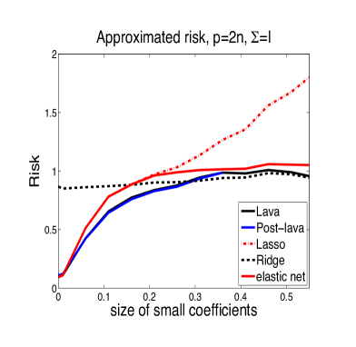
Refer to caption
Refer to caption
Refer to caption
Refer to caption
Figure 4. Simulation risk comparison with tuning done by minimizing SURE. In this figure, we report simulation estimates of risk functions of lava, post-lava, ridge, lasso, and elastic net in a Gaussian regression model with “sparse+dense” signal structure over the regression coefficients. We select tuning parameters by minimizing SURE. The size of “small coefficients” is shown on the horizontal axis. The size of these coefficients directly corresponds to the size of the “dense part” of the signal, with zero corresponding to the exactly sparse case. Relative risk plots the ratio of the risk of each estimator to the lava risk, R(θ,θ^e)/R(θ,θ^lava)R𝜃subscript^𝜃𝑒R𝜃subscript^𝜃lava\mathrm{R}(\theta,\widehat{\theta}_{e})/\mathrm{R}(\theta,\widehat{\theta}_{\mathrm{lava}}).
Refer to caption
Refer to caption
Refer to caption
Refer to caption
Figure 5. Simulation risk comparison with tuning done by 5-fold cross-validation. In this figure, we report simulation estimates of risk functions of lava, post-lava, ridge, lasso, and elastic net in a Gaussian regression model with “sparse+dense” signal structure over the regression coefficients. We select tuning parameters by 5-fold cross-validation. The size of “small coefficients” is shown on the horizontal axis. The size of these coefficients directly corresponds to the size of the “dense part” of the signal, with zero corresponding to the exactly sparse case. Relative risk plots the ratio of the risk of each estimator to the lava risk, R(θ,θ^e)/R(θ,θ^lava)R𝜃subscript^𝜃𝑒R𝜃subscript^𝜃lava\mathrm{R}(\theta,\widehat{\theta}_{e})/\mathrm{R}(\theta,\widehat{\theta}_{\mathrm{lava}}).

The comparisons are similar in both figures with lava and post-lava dominating the other procedures. It is particularly interesting to compare the performance of lava to lasso and ridge. The lava and post-lava estimators perform about as well as lasso when the signal is sparse and perform significantly better than lasso when the signal is non-sparse. The lava and post-lava estimators perform about as well as ridge when the signal is dense and perform much better than ridge when the signal is sparse. When the tuning parameters are selected via cross-validation, the post-lava performs slightly better than the lava when the model is sparse. The gain is somewhat more apparent in the independent design. Additional simulations are presented in our supplementary material (Chernozhukov et al. (2015)).

5. Discussion

We propose a new method, called “lava”, which is designed specifically to achieve good prediction and estimation performance in “sparse+dense” models. In such models, the high-dimensional parameter is represented as the sum of a sparse vector with a few large non-zero entries and a dense vector with many small entries. This structure renders traditional sparse or dense estimation methods, such as lasso or ridge, sub-optimal for prediction and other estimation purposes. The proposed approach thus complements other approaches to structured sparsity problems such as those considered in fused sparsity estimation (Tibshirani et al. (2005) and Chen and Dalalyan (2012)) and structured matrix decomposition problems (Candès et al. (2011), Chandrasekaran et al. (2011), Fan et al. (2013), and Klopp et al. (2014)).

There are a number of interesting research directions that remain to be considered. An immediate extension of the present results would be to consider semi-pivotal estimators akin to the root-lasso/scaled-lasso of Belloni et al. (2011) and Sun and Zhang (2012). For instance, we can define

θ^root-lavasubscript^𝜃root-lava\displaystyle\widehat{\theta}_{\textrm{root-lava}} :=assign\displaystyle:= β^+δ^,^𝛽^𝛿\displaystyle\widehat{\beta}+\widehat{\delta},
(β^,δ^)^𝛽^𝛿\displaystyle(\widehat{\beta},\widehat{\delta}) :=assign\displaystyle:= argminβ,δ,σ{12nσ2YX(β+δ)22+(1a)σ2+λ2β22+λ1δ1}.subscript𝛽𝛿𝜎12𝑛superscript𝜎2superscriptsubscriptnorm𝑌𝑋𝛽𝛿221𝑎𝜎2subscript𝜆2superscriptsubscriptnorm𝛽22subscript𝜆1subscriptnorm𝛿1\displaystyle\arg\min_{\beta,\delta,\sigma}\left\{\frac{1}{2n\sigma^{2}}\|Y-X(\beta+\delta)\|_{2}^{2}+\frac{(1-a)\sigma}{2}+\lambda_{2}\|\beta\|_{2}^{2}+\lambda_{1}\|\delta\|_{1}\right\}.

Thanks to the characterization of Theorem 3.1, the method can be implemented by applying root-lasso on appropriately transformed data. The present work could also be extended to accommodate non-Gaussian settings and settings with random designs, and it could also be extended beyond the mean regression problem to more general M- and Z- estimation problems, e.g., along the lines of Negahban et al. (2009).

Appendix A Proofs for Section 2

A.1. Proof of Lemma 2.1

Fixing δ𝛿\delta, the solution for β𝛽\beta is given by β^(δ)=(zδ)/(1+λ2)^𝛽𝛿𝑧𝛿1subscript𝜆2\widehat{\beta}(\delta)=(z-\delta)/(1+\lambda_{2}). Substituting back to the original problem, we obtain

d1(z)subscript𝑑1𝑧\displaystyle d_{1}(z) =\displaystyle= argminδ[zβ^(δ)δ]2+λ2|β^(δ)|2+λ1|δ|\displaystyle\arg\min_{\delta\in\mathbb{R}}[z-\widehat{\beta}(\delta)-\delta]^{2}+\lambda_{2}|\widehat{\beta}(\delta)|^{2}+\lambda_{1}|\delta|
=\displaystyle= argminδk(zδ)2+λ1|δ|.subscript𝛿𝑘superscript𝑧𝛿2subscript𝜆1𝛿\displaystyle\arg\min_{\delta\in\mathbb{R}}k(z-\delta)^{2}+\lambda_{1}|\delta|.

Hence d1(z)=(|z|λ1/(2k))+sign(z)subscript𝑑1𝑧subscript𝑧subscript𝜆12𝑘sign𝑧d_{1}(z)=(|z|-\lambda_{1}/(2k))_{+}\text{sign}(z), and d2(z)=β^(d1(z))=(z1d1(z))(1k)subscript𝑑2𝑧^𝛽subscript𝑑1𝑧subscript𝑧1subscript𝑑1𝑧1𝑘d_{2}(z)=\widehat{\beta}(d_{1}(z))=(z_{1}-d_{1}(z))(1-k). Consequently, dlava(z)=d1(z)+d2(z)=(1k)z+kd1(z)subscript𝑑lava𝑧subscript𝑑1𝑧subscript𝑑2𝑧1𝑘𝑧𝑘subscript𝑑1𝑧d_{\mathrm{lava}}(z)=d_{1}(z)+d_{2}(z)=(1-k)z+kd_{1}(z). \blacksquare

A.2. A Useful Lemma

The proofs rely on the following lemma.

Lemma A.1.

Consider the general piecewise linear function:

F(z)={hz+d,z>wez+m,|z|wfz+g,z<w.𝐹𝑧cases𝑧𝑑𝑧𝑤𝑒𝑧𝑚𝑧𝑤𝑓𝑧𝑔𝑧𝑤F(z)=\begin{cases}hz+d,&z>w\cr ez+m,&|z|\leq w\cr fz+g,&z<-w\end{cases}.

Suppose ZN(θ,σ2)similar-to𝑍𝑁𝜃superscript𝜎2Z\sim N(\theta,\sigma^{2}). Then

E[F(Z)2]Edelimited-[]𝐹superscript𝑍2\displaystyle{\mathrm{E}}[F(Z)^{2}] =\displaystyle= [σ2(h2w+h2θ+2dh)σ2(e2w+e2θ+2me)]ϕθ,σ(w)delimited-[]superscript𝜎2superscript2𝑤superscript2𝜃2𝑑superscript𝜎2superscript𝑒2𝑤superscript𝑒2𝜃2𝑚𝑒subscriptitalic-ϕ𝜃𝜎𝑤\displaystyle[\sigma^{2}(h^{2}w+h^{2}\theta+2dh)-\sigma^{2}(e^{2}w+e^{2}\theta+2me)]\phi_{\theta,\sigma}(w)
+[σ2(e2w+e2θ+2me)σ2(f2w+f2θ+2gf)]ϕθ,σ(w)delimited-[]superscript𝜎2superscript𝑒2𝑤superscript𝑒2𝜃2𝑚𝑒superscript𝜎2superscript𝑓2𝑤superscript𝑓2𝜃2𝑔𝑓subscriptitalic-ϕ𝜃𝜎𝑤\displaystyle+[\sigma^{2}(-e^{2}w+e^{2}\theta+2me)-\sigma^{2}(-f^{2}w+f^{2}\theta+2gf)]\phi_{\theta,\sigma}(-w)
+((hθ+d)2+h2σ2)Pθ,σ(Z>w)+((fθ+g)2+f2σ2)Pθ,σ(Z<w)superscript𝜃𝑑2superscript2superscript𝜎2subscriptP𝜃𝜎𝑍𝑤superscript𝑓𝜃𝑔2superscript𝑓2superscript𝜎2subscriptP𝜃𝜎𝑍𝑤\displaystyle+((h\theta+d)^{2}+h^{2}\sigma^{2}){\mathrm{P}}_{\theta,\sigma}(Z>w)+((f\theta+g)^{2}+f^{2}\sigma^{2}){\mathrm{P}}_{\theta,\sigma}(Z<-w)
+((eθ+m)2+e2σ2)Pθ,σ(|Z|<w).superscript𝑒𝜃𝑚2superscript𝑒2superscript𝜎2subscriptP𝜃𝜎𝑍𝑤\displaystyle+((e\theta+m)^{2}+e^{2}\sigma^{2}){\mathrm{P}}_{\theta,\sigma}(|Z|<w).
Proof.

We first consider an expectation of the following form: for any z1<z2subscript𝑧1subscript𝑧2-\infty\leq z_{1}<z_{2}\leq\infty, and a,b𝑎𝑏a,b\in\mathbb{R}, by integration by part,

E(θZ)(aZ+b)1{z1<Z<z2}=σ2z1z2θzσ2(az+b)ϕθ,σ(z)𝑑zE𝜃𝑍𝑎𝑍𝑏1subscript𝑧1𝑍subscript𝑧2superscript𝜎2superscriptsubscriptsubscript𝑧1subscript𝑧2𝜃𝑧superscript𝜎2𝑎𝑧𝑏subscriptitalic-ϕ𝜃𝜎𝑧differential-d𝑧\displaystyle{\mathrm{E}}(\theta-Z)(aZ+b)1\{z_{1}<Z<{z_{2}}\}=\sigma^{2}\int_{z_{1}}^{z_{2}}\frac{\theta-z}{\sigma^{2}}(az+b)\phi_{\theta,\sigma}(z)dz (A.1)
=σ2(az+b)ϕθ,σ(z)|z1z2σ2az1z2ϕθ,σ(z)𝑑zabsentevaluated-atsuperscript𝜎2𝑎𝑧𝑏subscriptitalic-ϕ𝜃𝜎𝑧subscript𝑧1subscript𝑧2superscript𝜎2𝑎superscriptsubscriptsubscript𝑧1subscript𝑧2subscriptitalic-ϕ𝜃𝜎𝑧differential-d𝑧\displaystyle=\sigma^{2}(az+b)\phi_{\theta,\sigma}(z)\big{|}_{z_{1}}^{z_{2}}-\sigma^{2}a\int_{z_{1}}^{z_{2}}\phi_{\theta,\sigma}(z)dz (A.2)
=σ2[(az2+b)ϕθ,σ(z2)(az1+b)ϕθ,σ(z1)]σ2aPθ,σ(z1<Z<z2).absentsuperscript𝜎2delimited-[]𝑎subscript𝑧2𝑏subscriptitalic-ϕ𝜃𝜎subscript𝑧2𝑎subscript𝑧1𝑏subscriptitalic-ϕ𝜃𝜎subscript𝑧1superscript𝜎2𝑎subscriptP𝜃𝜎subscript𝑧1𝑍subscript𝑧2\displaystyle=\sigma^{2}[(a{z_{2}}+b)\phi_{\theta,\sigma}(z_{2})-(a{z_{1}}+b)\phi_{\theta,\sigma}(z_{1})]-\sigma^{2}a{\mathrm{P}}_{\theta,\sigma}(z_{1}<Z<z_{2}). (A.3)

This result will be useful in the following calculations. Setting a=1𝑎1a=-1, b=θ𝑏𝜃b=\theta and a=0𝑎0a=0, b=2(θ+c)𝑏2𝜃𝑐b=-2(\theta+c) respectively yields

E(θZ)21{z1<Z<z2}=σ2[(θz2)ϕθ,σ(z2)(θz1)ϕθ,σ(z1)]+σ2Pθ,σ(z1<Z<z2).Esuperscript𝜃𝑍21subscript𝑧1𝑍subscript𝑧2superscript𝜎2delimited-[]𝜃subscript𝑧2subscriptitalic-ϕ𝜃𝜎subscript𝑧2𝜃subscript𝑧1subscriptitalic-ϕ𝜃𝜎subscript𝑧1superscript𝜎2subscriptP𝜃𝜎subscript𝑧1𝑍subscript𝑧2{\mathrm{E}}(\theta-Z)^{2}1\{z_{1}<Z<{z_{2}}\}=\sigma^{2}[(\theta-{z_{2}})\phi_{\theta,\sigma}(z_{2})-(\theta-{z_{1}})\phi_{\theta,\sigma}(z_{1})]+\sigma^{2}{\mathrm{P}}_{\theta,\sigma}(z_{1}<Z<z_{2}).
2E(Zθ)(θ+c)1{z1<Z<z2}=σ2[2(θ+c)ϕθ,σ(z2)+2(θ+c)ϕθ,σ(z1)].2E𝑍𝜃𝜃𝑐1subscript𝑧1𝑍subscript𝑧2superscript𝜎2delimited-[]2𝜃𝑐subscriptitalic-ϕ𝜃𝜎subscript𝑧22𝜃𝑐subscriptitalic-ϕ𝜃𝜎subscript𝑧12{\mathrm{E}}(Z-\theta)(\theta+c)1\{z_{1}<Z<{z_{2}}\}=\sigma^{2}[-2(\theta+c)\phi_{\theta,\sigma}(z_{2})+2(\theta+c)\phi_{\theta,\sigma}(z_{1})].

Therefore, for any constant c𝑐c,

E(Z+c)21{z1<Z<z2}Esuperscript𝑍𝑐21subscript𝑧1𝑍subscript𝑧2\displaystyle{\mathrm{E}}(Z+c)^{2}1\{z_{1}<Z<{z_{2}}\} =\displaystyle= E(θZ)21{z1<Z<z2}+(θ+c)2Pθ,σ(z1<Z<z2)Esuperscript𝜃𝑍21subscript𝑧1𝑍subscript𝑧2superscript𝜃𝑐2subscriptP𝜃𝜎subscript𝑧1𝑍subscript𝑧2\displaystyle{\mathrm{E}}(\theta-Z)^{2}1\{z_{1}<Z<{z_{2}}\}+(\theta+c)^{2}{\mathrm{P}}_{\theta,\sigma}(z_{1}<Z<{z_{2}}) (A.5)
+2E(Zθ)(θ+c)1{z1<Z<z2}2E𝑍𝜃𝜃𝑐1subscript𝑧1𝑍subscript𝑧2\displaystyle+2{\mathrm{E}}(Z-\theta)(\theta+c)1\{z_{1}<Z<{z_{2}}\}
=\displaystyle= σ2(z1+θ+2c)ϕθ,σ(z1)σ2(z2+θ+2c)ϕθ,σ(z2)superscript𝜎2subscript𝑧1𝜃2𝑐subscriptitalic-ϕ𝜃𝜎subscript𝑧1superscript𝜎2subscript𝑧2𝜃2𝑐subscriptitalic-ϕ𝜃𝜎subscript𝑧2\displaystyle\sigma^{2}(z_{1}+\theta+2c)\phi_{\theta,\sigma}(z_{1})-\sigma^{2}(z_{2}+\theta+2c)\phi_{\theta,\sigma}(z_{2}) (A.7)
+((θ+c)2+σ2)Pθ,σ(z1<Z<z2).superscript𝜃𝑐2superscript𝜎2subscriptP𝜃𝜎subscript𝑧1𝑍subscript𝑧2\displaystyle+((\theta+c)^{2}+\sigma^{2}){\mathrm{P}}_{\theta,\sigma}(z_{1}<Z<z_{2}).

If none of h,e,f𝑒𝑓h,e,f are zero, by setting z1=w,z2=formulae-sequencesubscript𝑧1𝑤subscript𝑧2z_{1}=w,z_{2}=\infty, c=d/h𝑐𝑑c=d/h; z1=,z2=w,c=g/fformulae-sequencesubscript𝑧1formulae-sequencesubscript𝑧2𝑤𝑐𝑔𝑓z_{1}=-\infty,z_{2}=-w,c=g/f and z1=w,z2=w,c=m/eformulae-sequencesubscript𝑧1𝑤formulae-sequencesubscript𝑧2𝑤𝑐𝑚𝑒z_{1}=-w,z_{2}=w,c=m/e respectively, we have

E(hZ+d)21{Z>w}=σ2(h2w+h2θ+2dh)ϕθ,σ(w)Esuperscript𝑍𝑑21𝑍𝑤superscript𝜎2superscript2𝑤superscript2𝜃2𝑑subscriptitalic-ϕ𝜃𝜎𝑤\displaystyle{\mathrm{E}}(hZ+d)^{2}1\{Z>w\}=\sigma^{2}(h^{2}w+h^{2}\theta+2dh)\phi_{\theta,\sigma}(w) (A.8)
+((θh+d)2+σ2h2)Pθ,σ(Z>w),superscript𝜃𝑑2superscript𝜎2superscript2subscriptP𝜃𝜎𝑍𝑤\displaystyle\hskip 108.405pt+((\theta h+d)^{2}+\sigma^{2}h^{2}){\mathrm{P}}_{\theta,\sigma}(Z>w), (A.9)
E(fZ+g)21{Z<w}=σ2(wf2+θf2+2gf)ϕθ,σ(w)Esuperscript𝑓𝑍𝑔21𝑍𝑤superscript𝜎2𝑤superscript𝑓2𝜃superscript𝑓22𝑔𝑓subscriptitalic-ϕ𝜃𝜎𝑤\displaystyle{\mathrm{E}}(fZ+g)^{2}1\{Z<-w\}=-\sigma^{2}(-wf^{2}+\theta f^{2}+2gf)\phi_{\theta,\sigma}(-w) (A.10)
+((θf+g)2+σ2f2)Pθ,σ(Z<w),superscript𝜃𝑓𝑔2superscript𝜎2superscript𝑓2subscriptP𝜃𝜎𝑍𝑤\displaystyle\hskip 108.405pt+((\theta f+g)^{2}+\sigma^{2}f^{2}){\mathrm{P}}_{\theta,\sigma}(Z<-w), (A.11)
E(eZ+m)21{|Z|<w}=σ2(we2+θe2+2me)ϕθ,σ(w)Esuperscript𝑒𝑍𝑚21𝑍𝑤superscript𝜎2𝑤superscript𝑒2𝜃superscript𝑒22𝑚𝑒subscriptitalic-ϕ𝜃𝜎𝑤\displaystyle{\mathrm{E}}(eZ+m)^{2}1\{|Z|<w\}=\sigma^{2}(-we^{2}+\theta e^{2}+2me)\phi_{\theta,\sigma}(-w) (A.12)
σ2(we2+θe2+2me)ϕθ,σ(w)superscript𝜎2𝑤superscript𝑒2𝜃superscript𝑒22𝑚𝑒subscriptitalic-ϕ𝜃𝜎𝑤\displaystyle\hskip 108.405pt-\sigma^{2}(we^{2}+\theta e^{2}+2me)\phi_{\theta,\sigma}(w) (A.13)
+((θe+m)2+σ2e2)Pθ,σ(|Z|<w).superscript𝜃𝑒𝑚2superscript𝜎2superscript𝑒2subscriptP𝜃𝜎𝑍𝑤\displaystyle\hskip 108.405pt+((\theta e+m)^{2}+\sigma^{2}e^{2}){\mathrm{P}}_{\theta,\sigma}(|Z|<w). (A.14)

If any of h,e,f𝑒𝑓h,e,f is zero, for instance, suppose h=00h=0, then E(hZ+d)21{Z>w}=d2Pθ,σ(Z>w),Esuperscript𝑍𝑑21𝑍𝑤superscript𝑑2subscriptP𝜃𝜎𝑍𝑤{\mathrm{E}}(hZ+d)^{2}1\{Z>w\}=d^{2}{\mathrm{P}}_{\theta,\sigma}(Z>w), which can also be written as the first equality of (A.8). Similarly, when either e=0𝑒0e=0 or f=0𝑓0f=0, (A.8) still holds.

Therefore, summing up the three terms of (A.8) yields the desired result. \blacksquare

A.3. Proof of Theorem 2.1

Recall that θ^lava=(1k)Z+kdlasso(Z)subscript^𝜃lava1𝑘𝑍𝑘subscript𝑑lasso𝑍\widehat{\theta}_{\text{lava}}=(1-k)Z+k{d}_{\mathrm{lasso}}(Z) is a weighted average of Z𝑍Z and the soft-thresholded estimator with shrinkage parameters λ1/(2k)subscript𝜆12𝑘\lambda_{1}/(2k) and k=λ2/(1+λ2)𝑘subscript𝜆21subscript𝜆2k=\lambda_{2}/(1+\lambda_{2}). Since dlasso(Z)subscript𝑑lasso𝑍{d}_{\mathrm{lasso}}(Z) is a soft-thresholding estimator, results from Donoho and Johnstone (1995) give that

E[(Zθ)dlasso(Z)]=σ2Pθ,σ(|Z|>λ1/(2k)).Edelimited-[]𝑍𝜃subscript𝑑lasso𝑍superscript𝜎2subscriptP𝜃𝜎𝑍subscript𝜆12𝑘{\mathrm{E}}[(Z-\theta){d}_{\mathrm{lasso}}(Z)]=\sigma^{2}{\mathrm{P}}_{\theta,\sigma}(|Z|>\lambda_{1}/(2k)).

Therefore, for w=λ1/(2k)𝑤subscript𝜆12𝑘w=\lambda_{1}/(2k),

2E[(Zθ)dlava(Z)]=2(1k)σ2+2kσ2Pθ,σ(|Z|>w).2Edelimited-[]𝑍𝜃subscript𝑑lava𝑍21𝑘superscript𝜎22𝑘superscript𝜎2subscriptP𝜃𝜎𝑍𝑤\displaystyle 2{\mathrm{E}}[(Z-\theta)d_{\mathrm{lava}}(Z)]=2(1-k)\sigma^{2}+2k\sigma^{2}{\mathrm{P}}_{\theta,\sigma}(|Z|>w). (A.15)

Next we verify that

E(Zdlava(Z))2=k2(w+θ)ϕθ,σ(w)σ2+k2(θw)ϕθ,σ(w)σ2+(λ12/4)Pθ,σ(|Z|>w)+k2(θ2+σ2)Pθ,σ(|Z|<w).Esuperscript𝑍subscript𝑑lava𝑍2absentsuperscript𝑘2𝑤𝜃subscriptitalic-ϕ𝜃𝜎𝑤superscript𝜎2superscript𝑘2𝜃𝑤subscriptitalic-ϕ𝜃𝜎𝑤superscript𝜎2missing-subexpressionsuperscriptsubscript𝜆124subscriptP𝜃𝜎𝑍𝑤superscript𝑘2superscript𝜃2superscript𝜎2subscriptP𝜃𝜎𝑍𝑤\begin{array}[]{ll}{\mathrm{E}}(Z-{d}_{\mathrm{lava}}(Z))^{2}&=-k^{2}(w+\theta)\phi_{\theta,\sigma}(w)\sigma^{2}+k^{2}(\theta-w)\phi_{\theta,\sigma}(-w)\sigma^{2}\cr&+(\lambda_{1}^{2}/4){\mathrm{P}}_{\theta,\sigma}(|Z|>w)+k^{2}(\theta^{2}+\sigma^{2}){\mathrm{P}}_{\theta,\sigma}(|Z|<w).\end{array} (A.16)

By definition,

dlava(z)zsubscript𝑑lava𝑧𝑧\displaystyle{d}_{\mathrm{lava}}(z)-z =\displaystyle= {λ1/2,z>λ1/(2k),kz,λ1/(2k)<zλ1/(2k),λ1/2,z<λ1/(2k).casessubscript𝜆12𝑧subscript𝜆12𝑘𝑘𝑧subscript𝜆12𝑘𝑧subscript𝜆12𝑘subscript𝜆12𝑧subscript𝜆12𝑘\displaystyle\begin{cases}-\lambda_{1}/2,&z>\lambda_{1}/(2k),\\ -kz,&-\lambda_{1}/(2k)<z\leq\lambda_{1}/(2k),\\ \lambda_{1}/2,&z<-\lambda_{1}/(2k).\end{cases} (A.17)

Let F(z)=dlava(z)z𝐹𝑧subscript𝑑lava𝑧𝑧F(z)={d}_{\mathrm{lava}}(z)-z. The claim then follows from applying Lemma A.1 by setting h=f=m=0𝑓𝑚0h=f=m=0, d=λ1/2𝑑subscript𝜆12d=-\lambda_{1}/2, e=k𝑒𝑘e=-k, g=λ1/2𝑔subscript𝜆12g=\lambda_{1}/2, and w=λ1/(2k)𝑤subscript𝜆12𝑘w=\lambda_{1}/(2k).

Hence

E(Zdlava(Z))2Esuperscript𝑍subscript𝑑lava𝑍2\displaystyle{\mathrm{E}}(Z-d_{\mathrm{lava}}(Z))^{2} =\displaystyle= k2(w+θ)ϕθ,σ(w)σ2+k2(θw)ϕθ,σ(w)σ2superscript𝑘2𝑤𝜃subscriptitalic-ϕ𝜃𝜎𝑤superscript𝜎2superscript𝑘2𝜃𝑤subscriptitalic-ϕ𝜃𝜎𝑤superscript𝜎2\displaystyle-k^{2}(w+\theta)\phi_{\theta,\sigma}(w)\sigma^{2}+k^{2}(\theta-w)\phi_{\theta,\sigma}(-w)\sigma^{2}
+(λ12/4)Pθ,σ(|Z|>w)+k2(θ2+σ2)Pθ,σ(|Z|<w).superscriptsubscript𝜆124subscriptP𝜃𝜎𝑍𝑤superscript𝑘2superscript𝜃2superscript𝜎2subscriptP𝜃𝜎𝑍𝑤\displaystyle+(\lambda_{1}^{2}/4){\mathrm{P}}_{\theta,\sigma}(|Z|>w)+k^{2}(\theta^{2}+\sigma^{2}){\mathrm{P}}_{\theta,\sigma}(|Z|<w).

The risk of lasso is obtained from setting λ2=subscript𝜆2\lambda_{2}=\infty and λ1=λlsubscript𝜆1subscript𝜆𝑙\lambda_{1}=\lambda_{l} in the lava risk. The risk of ridge is obtained from setting λ1=subscript𝜆1\lambda_{1}=\infty and λ2=λrsubscript𝜆2subscript𝜆𝑟\lambda_{2}=\lambda_{r} in the lava risk.

As for the risk of post-lava, note that

dpost-lava(z)θ={zθ,|z|>λ1/(2k)(1k)zθ,|z|λ1/(2k).subscript𝑑post-lava𝑧𝜃cases𝑧𝜃𝑧subscript𝜆12𝑘1𝑘𝑧𝜃𝑧subscript𝜆12𝑘\displaystyle{d}_{\textrm{post-lava}}(z)-\theta=\begin{cases}z-\theta,&|z|>\lambda_{1}/(2k)\\ (1-k)z-\theta,&|z|\leq\lambda_{1}/(2k).\end{cases}

Hence applying Lemma A.1 to F(z)=dpost-lava(z)θ𝐹𝑧subscript𝑑post-lava𝑧𝜃F(z)={d}_{\textrm{post-lava}}(z)-\theta, i.e. by setting h=f=1,e=1kformulae-sequence𝑓1𝑒1𝑘h=f=1,e=1-k and d=m=g=θ𝑑𝑚𝑔𝜃d=m=g=-\theta, we obtain:

R(θ,θ^post-lava)𝑅𝜃subscript^𝜃post-lava\displaystyle R(\theta,\widehat{\theta}_{\text{post-lava}}) =\displaystyle= σ2[k2w+2kwk2θ]ϕθ,σ(w)+σ2[k2w+2kw+k2θ]ϕθ,σ(w)superscript𝜎2delimited-[]superscript𝑘2𝑤2𝑘𝑤superscript𝑘2𝜃subscriptitalic-ϕ𝜃𝜎𝑤superscript𝜎2delimited-[]superscript𝑘2𝑤2𝑘𝑤superscript𝑘2𝜃subscriptitalic-ϕ𝜃𝜎𝑤\displaystyle\sigma^{2}[-k^{2}w+2kw-k^{2}\theta]\phi_{\theta,\sigma}(w)+\sigma^{2}[-k^{2}w+2kw+k^{2}\theta]\phi_{\theta,\sigma}(-w)
+σ2Pθ,σ(|Z|>w)+(k2θ2+(1k)2σ2)Pθ,σ(|Z|<w).superscript𝜎2subscriptP𝜃𝜎𝑍𝑤superscript𝑘2superscript𝜃2superscript1𝑘2superscript𝜎2subscriptP𝜃𝜎𝑍𝑤\displaystyle+\sigma^{2}{\mathrm{P}}_{\theta,\sigma}(|Z|>w)+(k^{2}\theta^{2}+(1-k)^{2}\sigma^{2}){\mathrm{P}}_{\theta,\sigma}(|Z|<w).

Finally, the elastic net shrinkage is given by

denet(z)=11+λ2(|z|λ1/2)+sgn(z).subscript𝑑enet𝑧11subscript𝜆2subscript𝑧subscript𝜆12sgn𝑧{d}_{\mathrm{enet}}(z)=\frac{1}{1+\lambda_{2}}(|z|-\lambda_{1}/2)_{+}\text{sgn}(z).

The risk of elastic net then follows from Lemma A.1 by setting F(z)=denet(z)θ𝐹𝑧subscript𝑑enet𝑧𝜃F(z)={d}_{\mathrm{enet}}(z)-\theta, w=λ1/2,h=f=1/(1+λ2),e=0formulae-sequenceformulae-sequence𝑤subscript𝜆12𝑓11subscript𝜆2𝑒0w=\lambda_{1}/2,h=f=1/(1+\lambda_{2}),e=0, d=λ1/(2(1+λ2))θ𝑑subscript𝜆121subscript𝜆2𝜃d=-\lambda_{1}/(2(1+\lambda_{2}))-\theta and g=λ1/(2(1+λ2))θ𝑔subscript𝜆121subscript𝜆2𝜃g=\lambda_{1}/(2(1+\lambda_{2}))-\theta. \blacksquare

A.4. Proof of Lemma 2.2

For θ^lava=(θ^lava,j)j=1psubscript^𝜃lavasuperscriptsubscriptsubscript^𝜃lava𝑗𝑗1𝑝\widehat{\theta}_{\text{lava}}=(\widehat{\theta}_{\mathrm{lava},j})_{j=1}^{p}, we have

Eθ^lavaθ22=j=1pR(θj,θ^lava,j).Esuperscriptsubscriptnormsubscript^𝜃lava𝜃22superscriptsubscript𝑗1𝑝𝑅subscript𝜃𝑗subscript^𝜃lava𝑗{\mathrm{E}}\|\widehat{\theta}_{\text{lava}}-\theta\|_{2}^{2}=\sum_{j=1}^{p}R(\theta_{j},\widehat{\theta}_{\mathrm{lava},j}).

We now bound R(θj,θ^lava,j)𝑅subscript𝜃𝑗subscript^𝜃lava𝑗R(\theta_{j},\widehat{\theta}_{\mathrm{lava},j}) uniformly over j=1,,p𝑗1𝑝j=1,...,p. We have that

θ^lava,jθj=(1k)Zj+kδ^jθj=[(1k)(Zjδj)βj]+k(δ^jδj),k=λ21+λ2,formulae-sequencesubscript^𝜃lava𝑗subscript𝜃𝑗1𝑘subscript𝑍𝑗𝑘subscript^𝛿𝑗subscript𝜃𝑗delimited-[]1𝑘subscript𝑍𝑗subscript𝛿𝑗subscript𝛽𝑗𝑘subscript^𝛿𝑗subscript𝛿𝑗𝑘subscript𝜆21subscript𝜆2\widehat{\theta}_{\text{lava},j}-\theta_{j}=(1-k)Z_{j}+k\widehat{\delta}_{j}-\theta_{j}=[(1-k)(Z_{j}-\delta_{j})-\beta_{j}]+k(\widehat{\delta}_{j}-\delta_{j}),\quad k=\frac{\lambda_{2}}{1+\lambda_{2}},

where δ^j=dlasso(Zj)subscript^𝛿𝑗subscript𝑑lassosubscript𝑍𝑗\widehat{\delta}_{j}={d}_{\mathrm{lasso}}(Z_{j}) with penalty level λ1subscript𝜆1\lambda_{1}. Hence

E(θ^jθj)2Esuperscriptsubscript^𝜃𝑗subscript𝜃𝑗2\displaystyle{\mathrm{E}}(\widehat{\theta}_{j}-\theta_{j})^{2} =E[(1k)(Zjδj)βj]2I+k2E(δ^jδj)2IIabsentsubscriptEsuperscriptdelimited-[]1𝑘subscript𝑍𝑗subscript𝛿𝑗subscript𝛽𝑗2𝐼subscriptsuperscript𝑘2Esuperscriptsubscript^𝛿𝑗subscript𝛿𝑗2𝐼𝐼\displaystyle=\underbrace{{\mathrm{E}}[(1-k)(Z_{j}-\delta_{j})-\beta_{j}]^{2}}_{I}+\underbrace{k^{2}{\mathrm{E}}(\widehat{\delta}_{j}-\delta_{j})^{2}}_{II}
+2kE{(δ^jδj)[(1k)(Zjδj)βj]}IIIsubscript2𝑘Esubscript^𝛿𝑗subscript𝛿𝑗delimited-[]1𝑘subscript𝑍𝑗subscript𝛿𝑗subscript𝛽𝑗𝐼𝐼𝐼\displaystyle+\underbrace{2k{\mathrm{E}}\{(\widehat{\delta}_{j}-\delta_{j})[(1-k)(Z_{j}-\delta_{j})-\beta_{j}]\}}_{III}

Bounding I. Note that ZjδjN(βj,σ2)similar-tosubscript𝑍𝑗subscript𝛿𝑗𝑁subscript𝛽𝑗superscript𝜎2Z_{j}-\delta_{j}\sim N(\beta_{j},\sigma^{2}). The first term Gj(1k)(Zjδj)βjsubscript𝐺𝑗1𝑘subscript𝑍𝑗subscript𝛿𝑗subscript𝛽𝑗G_{j}\equiv(1-k)(Z_{j}-\delta_{j})-\beta_{j} is thus the bias of a ridge estimator, with EGj2=(1k)2σ2+k2βj2Esuperscriptsubscript𝐺𝑗2superscript1𝑘2superscript𝜎2superscript𝑘2superscriptsubscript𝛽𝑗2{\mathrm{E}}G_{j}^{2}=(1-k)^{2}\sigma^{2}+k^{2}\beta_{j}^{2}.

Bounding II. Note that λ1=2σΦ1(1c/(2p))subscript𝜆12𝜎superscriptΦ11𝑐2𝑝\lambda_{1}=2\sigma{\Phi^{-1}(1-c/(2p))}. By Mill’s ratio inequality, as long as 2pπc2logp1πc22𝑝𝜋superscript𝑐2𝑝1𝜋superscript𝑐2\frac{2p}{\pi c^{2}}\geq{\log p}\geq\frac{1}{\pi c^{2}}, 22logp>λ1/σ>2logp22𝑝subscript𝜆1𝜎2𝑝2\sqrt{2\log p}>\lambda_{1}/\sigma>2\sqrt{\log p}. In addition,

E(δ^jδj)2=E(δ^jθj)2+βj2+2E(δ^jθj)βj.Esuperscriptsubscript^𝛿𝑗subscript𝛿𝑗2Esuperscriptsubscript^𝛿𝑗subscript𝜃𝑗2superscriptsubscript𝛽𝑗22Esubscript^𝛿𝑗subscript𝜃𝑗subscript𝛽𝑗{\mathrm{E}}(\widehat{\delta}_{j}-\delta_{j})^{2}={\mathrm{E}}(\widehat{\delta}_{j}-\theta_{j})^{2}+\beta_{j}^{2}+2{\mathrm{E}}(\widehat{\delta}_{j}-\theta_{j})\beta_{j}.

Since ZjN(θj,σ2)similar-tosubscript𝑍𝑗𝑁subscript𝜃𝑗superscript𝜎2Z_{j}\sim N(\theta_{j},\sigma^{2}), by Theorem 2.1 with λl=λ1/k>2σlogpsubscript𝜆𝑙subscript𝜆1𝑘2𝜎𝑝\lambda_{l}=\lambda_{1}/k>2\sigma\sqrt{\log p} (since k1𝑘1k\leq 1),

E(δ^jθj)2Esuperscriptsubscript^𝛿𝑗subscript𝜃𝑗2\displaystyle{\mathrm{E}}(\widehat{\delta}_{j}-\theta_{j})^{2} =\displaystyle= (λl/2+θj)ϕθj,σ(λl/2)σ2+(θjλl/2)ϕθj,σ(λl/2)σ2subscript𝜆𝑙2subscript𝜃𝑗subscriptitalic-ϕsubscript𝜃𝑗𝜎subscript𝜆𝑙2superscript𝜎2subscript𝜃𝑗subscript𝜆𝑙2subscriptitalic-ϕsubscript𝜃𝑗𝜎subscript𝜆𝑙2superscript𝜎2\displaystyle-(\lambda_{l}/2+\theta_{j})\phi_{\theta_{j},\sigma}(\lambda_{l}/2)\sigma^{2}+(\theta_{j}-\lambda_{l}/2)\phi_{\theta_{j},\sigma}(-\lambda_{l}/2)\sigma^{2}
+(λl2/4+σ2)Pθj,σ(|Zj|>λl/2)+θj2Pθj,σ(|Zj|<λl/2)superscriptsubscript𝜆𝑙24superscript𝜎2subscriptPsubscript𝜃𝑗𝜎subscript𝑍𝑗subscript𝜆𝑙2superscriptsubscript𝜃𝑗2subscriptPsubscript𝜃𝑗𝜎subscript𝑍𝑗subscript𝜆𝑙2\displaystyle+(\lambda_{l}^{2}/4+\sigma^{2}){\mathrm{P}}_{\theta_{j},\sigma}(|Z_{j}|>\lambda_{l}/2)+\theta_{j}^{2}{\mathrm{P}}_{\theta_{j},\sigma}(|Z_{j}|<\lambda_{l}/2)
(1)subscript1\displaystyle\leq_{(1)} (λl2/4+σ2)σ2π(λl/2θj)e(λl/2θj)2/2σ2superscriptsubscript𝜆𝑙24superscript𝜎2𝜎2𝜋subscript𝜆𝑙2subscript𝜃𝑗superscript𝑒superscriptsubscript𝜆𝑙2subscript𝜃𝑗22superscript𝜎2\displaystyle(\lambda_{l}^{2}/4+\sigma^{2})\frac{\sigma}{\sqrt{2\pi}(\lambda_{l}/2-\theta_{j})}e^{-(\lambda_{l}/2-\theta_{j})^{2}/2\sigma^{2}}
+(λl2/4+σ2)σ2π(λl/2+θj)e(λl/2+θj)22σ2+θj2Pθj,σ(|Zj|<λl/2)superscriptsubscript𝜆𝑙24superscript𝜎2𝜎2𝜋subscript𝜆𝑙2subscript𝜃𝑗superscript𝑒superscriptsubscript𝜆𝑙2subscript𝜃𝑗22superscript𝜎2superscriptsubscript𝜃𝑗2subscriptPsubscript𝜃𝑗𝜎subscript𝑍𝑗subscript𝜆𝑙2\displaystyle+(\lambda_{l}^{2}/4+\sigma^{2})\frac{\sigma}{\sqrt{2\pi}(\lambda_{l}/2+\theta_{j})}e^{-\frac{(\lambda_{l}/2+\theta_{j})^{2}}{2\sigma^{2}}}+\theta_{j}^{2}{\mathrm{P}}_{\theta_{j},\sigma}(|Z_{j}|<\lambda_{l}/2)
(2)subscript2\displaystyle\leq_{(2)} 2×(λl2/4+σ2)4σ2πλleλl2/(32σ2)+θj22superscriptsubscript𝜆𝑙24superscript𝜎24𝜎2𝜋subscript𝜆𝑙superscript𝑒superscriptsubscript𝜆𝑙232superscript𝜎2superscriptsubscript𝜃𝑗2\displaystyle 2\times(\lambda_{l}^{2}/4+\sigma^{2})\frac{4\sigma}{\sqrt{2\pi}\lambda_{l}}e^{-\lambda_{l}^{2}/(32\sigma^{2})}+\theta_{j}^{2}
(3)subscript3\displaystyle\leq_{(3)} 4λlσ22πσeλl2/(32σ2)+θj24subscript𝜆𝑙superscript𝜎22𝜋𝜎superscript𝑒superscriptsubscript𝜆𝑙232superscript𝜎2superscriptsubscript𝜃𝑗2\displaystyle\frac{4\lambda_{l}\sigma^{2}}{\sqrt{2\pi}\sigma}e^{-\lambda_{l}^{2}/(32\sigma^{2})}+\theta_{j}^{2}
(4)subscript4\displaystyle\leq_{(4)} 4σ22πeλl2/(64σ2)+θj24σ22πp(1/4)2+θj24superscript𝜎22𝜋superscript𝑒superscriptsubscript𝜆𝑙264superscript𝜎2superscriptsubscript𝜃𝑗24superscript𝜎22𝜋superscript𝑝superscript142superscriptsubscript𝜃𝑗2\displaystyle\frac{4\sigma^{2}}{\sqrt{2\pi}}e^{-\lambda_{l}^{2}/(64\sigma^{2})}+\theta_{j}^{2}\leq\frac{4\sigma^{2}}{\sqrt{2\pi}p^{(1/4)^{2}}}+\theta_{j}^{2}

where (1) follows from the Mill’s ratio inequality: xet2/2𝑑tx1ex2/2superscriptsubscript𝑥superscript𝑒superscript𝑡22differential-d𝑡superscript𝑥1superscript𝑒superscript𝑥22\int_{x}^{\infty}e^{-t^{2}/2}dt\leq x^{-1}e^{-x^{2}/2} for x0𝑥0x\geq 0. Also note that λl/2±θj>0plus-or-minussubscript𝜆𝑙2subscript𝜃𝑗0\lambda_{l}/2\pm\theta_{j}>0 since θ<Msubscriptnorm𝜃𝑀\|\theta\|_{\infty}<M and σlogp>2M𝜎𝑝2𝑀\sigma\sqrt{\log p}>2M. Hence we can apply the Mill’s ratio inequality respectively on Pθj,σ(Zj>λl/2)subscriptPsubscript𝜃𝑗𝜎subscript𝑍𝑗subscript𝜆𝑙2{\mathrm{P}}_{\theta_{j},\sigma}(Z_{j}>\lambda_{l}/2) and Pθj,σ(Zj<λl/2)subscriptPsubscript𝜃𝑗𝜎subscript𝑍𝑗subscript𝜆𝑙2{\mathrm{P}}_{\theta_{j},\sigma}(Z_{j}<-\lambda_{l}/2). In addition, the first two terms on the right hand side are negative. (2) is due to λl/2±θj>λl/4plus-or-minussubscript𝜆𝑙2subscript𝜃𝑗subscript𝜆𝑙4\lambda_{l}/2\pm\theta_{j}>\lambda_{l}/4 since |θj|<Msubscript𝜃𝑗𝑀|\theta_{j}|<M and σlogp>2M𝜎𝑝2𝑀\sigma\sqrt{\log p}>2M. (3) follows since 4σ2λl24superscript𝜎2superscriptsubscript𝜆𝑙24\sigma^{2}\leq\lambda_{l}^{2} when pe𝑝𝑒p\geq e. Finally, for any a>0𝑎0a>0, and any x>1+a1𝑥1superscript𝑎1x>1+a^{-1}, ax2>logx𝑎superscript𝑥2𝑥ax^{2}>\log x. Set a=641𝑎superscript641a=64^{-1}; when logp>33𝑝33\sqrt{\log p}>33, log(λl/σ)<λl2/(64σ2)subscript𝜆𝑙𝜎superscriptsubscript𝜆𝑙264superscript𝜎2\log(\lambda_{l}/\sigma)<\lambda_{l}^{2}/(64\sigma^{2}). Hence λlσeλl2/(32σ2)eλl2/(64σ2)subscript𝜆𝑙𝜎superscript𝑒superscriptsubscript𝜆𝑙232superscript𝜎2superscript𝑒superscriptsubscript𝜆𝑙264superscript𝜎2\frac{\lambda_{l}}{\sigma}e^{-\lambda_{l}^{2}/(32\sigma^{2})}\leq e^{-\lambda_{l}^{2}/(64\sigma^{2})}, which gives (4). Therefore,

j=1pE(δ^jθj)24pσ22πp(1/4)2+θ22.superscriptsubscript𝑗1𝑝Esuperscriptsubscript^𝛿𝑗subscript𝜃𝑗24𝑝superscript𝜎22𝜋superscript𝑝superscript142superscriptsubscriptnorm𝜃22\sum_{j=1}^{p}{\mathrm{E}}(\widehat{\delta}_{j}-\theta_{j})^{2}\leq\frac{4p\sigma^{2}}{\sqrt{2\pi}p^{(1/4)^{2}}}+\|\theta\|_{2}^{2}.

On the other hand, applying (A.1) and by the same arguments as above, uniformly for j=1,,p𝑗1𝑝j=1,...,p,

|Eδ^j|Esubscript^𝛿𝑗\displaystyle|{\mathrm{E}}\widehat{\delta}_{j}| =\displaystyle= |σ2[ϕθj,σ(λl/2)ϕθj,σ(λl/2)]+(θjλl/2)Pθj,σ(Zj>λl/2)\displaystyle|\sigma^{2}[\phi_{\theta_{j},\sigma}(\lambda_{l}/2)-\phi_{\theta_{j},\sigma}(-\lambda_{l}/2)]+(\theta_{j}-\lambda_{l}/2){\mathrm{P}}_{\theta_{j},\sigma}(Z_{j}>\lambda_{l}/2)
+(θj+λl/2)Pθj,σ(Zj<λl/2)|\displaystyle+(\theta_{j}+\lambda_{l}/2){\mathrm{P}}_{\theta_{j},\sigma}(Z_{j}<-\lambda_{l}/2)|
\displaystyle\leq 8σ2πeλl2/(32σ2)8σ2π1p1/8.8𝜎2𝜋superscript𝑒superscriptsubscript𝜆𝑙232superscript𝜎28𝜎2𝜋1superscript𝑝18\displaystyle\frac{8\sigma}{\sqrt{2\pi}}e^{-\lambda_{l}^{2}/(32\sigma^{2})}\leq\frac{8\sigma}{\sqrt{2\pi}}\frac{1}{p^{1/8}}.

Moreover, θ22+β222j=1pθjβj=δ22superscriptsubscriptnorm𝜃22superscriptsubscriptnorm𝛽222superscriptsubscript𝑗1𝑝subscript𝜃𝑗subscript𝛽𝑗superscriptsubscriptnorm𝛿22\|\theta\|_{2}^{2}+\|\beta\|_{2}^{2}-2\sum_{j=1}^{p}\theta_{j}\beta_{j}=\|\delta\|_{2}^{2}. Hence

j=1pE(δ^jδj)2superscriptsubscript𝑗1𝑝Esuperscriptsubscript^𝛿𝑗subscript𝛿𝑗2\displaystyle\sum_{j=1}^{p}{\mathrm{E}}(\widehat{\delta}_{j}-\delta_{j})^{2} \displaystyle\leq j=1pE(δ^jθj)2+β222j=1pθjβj+2j=1pEδ^jβjsuperscriptsubscript𝑗1𝑝Esuperscriptsubscript^𝛿𝑗subscript𝜃𝑗2superscriptsubscriptnorm𝛽222superscriptsubscript𝑗1𝑝subscript𝜃𝑗subscript𝛽𝑗2superscriptsubscript𝑗1𝑝Esubscript^𝛿𝑗subscript𝛽𝑗\displaystyle\sum_{j=1}^{p}{\mathrm{E}}(\widehat{\delta}_{j}-\theta_{j})^{2}+\|\beta\|_{2}^{2}-2\sum_{j=1}^{p}\theta_{j}\beta_{j}+2\sum_{j=1}^{p}{\mathrm{E}}\widehat{\delta}_{j}\beta_{j}
\displaystyle\leq δ22+4pσ22πp1/16+β10σp2πp1/8.superscriptsubscriptnorm𝛿224𝑝superscript𝜎22𝜋superscript𝑝116subscriptnorm𝛽10𝜎𝑝2𝜋superscript𝑝18\displaystyle\|\delta\|_{2}^{2}+\frac{4p\sigma^{2}}{\sqrt{2\pi}p^{1/16}}+\|\beta\|_{\infty}\frac{10\sigma p}{\sqrt{2\pi}p^{1/8}}.

Bounding III. By Donoho and Johnstone (1995), E[(θjZj)δ^j]=σ2Pθj,σ(|Zj|>λ1/(2k)).Edelimited-[]subscript𝜃𝑗subscript𝑍𝑗subscript^𝛿𝑗superscript𝜎2subscriptPsubscript𝜃𝑗𝜎subscript𝑍𝑗subscript𝜆12𝑘{\mathrm{E}}[(\theta_{j}-Z_{j})\widehat{\delta}_{j}]=-\sigma^{2}{\mathrm{P}}_{\theta_{j},\sigma}(|Z_{j}|>\lambda_{1}/(2k)). Hence (note that E(Zjθj)=0Esubscript𝑍𝑗subscript𝜃𝑗0{\mathrm{E}}(Z_{j}-\theta_{j})=0)

E[(δ^jδj)(Zjδj)]Edelimited-[]subscript^𝛿𝑗subscript𝛿𝑗subscript𝑍𝑗subscript𝛿𝑗\displaystyle{\mathrm{E}}[(\widehat{\delta}_{j}-\delta_{j})(Z_{j}-\delta_{j})] =\displaystyle= E[δ^j(Zjθj)]+E[δ^jδj)βj]\displaystyle{\mathrm{E}}[\widehat{\delta}_{j}(Z_{j}-\theta_{j})]+{\mathrm{E}}[\widehat{\delta}_{j}-\delta_{j})\beta_{j}]
=\displaystyle= σ2Pθj,σ(|Zj|>λ1/(2k))+βjEδ^jδjβjsuperscript𝜎2subscriptPsubscript𝜃𝑗𝜎subscript𝑍𝑗subscript𝜆12𝑘subscript𝛽𝑗Esubscript^𝛿𝑗subscript𝛿𝑗subscript𝛽𝑗\displaystyle\sigma^{2}{\mathrm{P}}_{\theta_{j},\sigma}(|Z_{j}|>\lambda_{1}/(2k))+\beta_{j}{\mathrm{E}}\widehat{\delta}_{j}-\delta_{j}\beta_{j}
\displaystyle\leq 2σ24σ2πλleλl2/(32σ2)+βjEδ^jδjβj2superscript𝜎24𝜎2𝜋subscript𝜆𝑙superscript𝑒superscriptsubscript𝜆𝑙232superscript𝜎2subscript𝛽𝑗Esubscript^𝛿𝑗subscript𝛿𝑗subscript𝛽𝑗\displaystyle 2\sigma^{2}\frac{4\sigma}{\sqrt{2\pi}\lambda_{l}}e^{-\lambda_{l}^{2}/(32\sigma^{2})}+\beta_{j}{\mathrm{E}}\widehat{\delta}_{j}-\delta_{j}\beta_{j}
\displaystyle\leq 4σ22π1logp1p1/8+βjEδ^jδjβj,4superscript𝜎22𝜋1𝑝1superscript𝑝18subscript𝛽𝑗Esubscript^𝛿𝑗subscript𝛿𝑗subscript𝛽𝑗\displaystyle\frac{4\sigma^{2}}{\sqrt{2\pi}}\frac{1}{\sqrt{\log p}}\frac{1}{p^{1/8}}+\beta_{j}{\mathrm{E}}\widehat{\delta}_{j}-\delta_{j}\beta_{j},

implying

j=1pE{(δ^jδj)[(1k)(Zjδj)βj]}superscriptsubscript𝑗1𝑝Esubscript^𝛿𝑗subscript𝛿𝑗delimited-[]1𝑘subscript𝑍𝑗subscript𝛿𝑗subscript𝛽𝑗\displaystyle\sum_{j=1}^{p}{\mathrm{E}}\{(\widehat{\delta}_{j}-\delta_{j})[(1-k)(Z_{j}-\delta_{j})-\beta_{j}]\}
=\displaystyle= (1k)j=1pE[(δ^jδj)(Zjδj)]j=1pEδ^jβj+j=1pδjβj1𝑘superscriptsubscript𝑗1𝑝Edelimited-[]subscript^𝛿𝑗subscript𝛿𝑗subscript𝑍𝑗subscript𝛿𝑗superscriptsubscript𝑗1𝑝Esubscript^𝛿𝑗subscript𝛽𝑗superscriptsubscript𝑗1𝑝subscript𝛿𝑗subscript𝛽𝑗\displaystyle(1-k)\sum_{j=1}^{p}{\mathrm{E}}[(\widehat{\delta}_{j}-\delta_{j})(Z_{j}-\delta_{j})]-\sum_{j=1}^{p}{\mathrm{E}}\widehat{\delta}_{j}\beta_{j}+\sum_{j=1}^{p}\delta_{j}\beta_{j}
\displaystyle\leq (1k)4σ22πplogp1p1/8+(1k)j=1pβjEδ^jj=1pEδ^jβj+kj=1pδjβj1𝑘4superscript𝜎22𝜋𝑝𝑝1superscript𝑝181𝑘superscriptsubscript𝑗1𝑝subscript𝛽𝑗Esubscript^𝛿𝑗superscriptsubscript𝑗1𝑝Esubscript^𝛿𝑗subscript𝛽𝑗𝑘superscriptsubscript𝑗1𝑝subscript𝛿𝑗subscript𝛽𝑗\displaystyle(1-k)\frac{4\sigma^{2}}{\sqrt{2\pi}}\frac{p}{\sqrt{\log p}}\frac{1}{p^{1/8}}+(1-k)\sum_{j=1}^{p}\beta_{j}{\mathrm{E}}\widehat{\delta}_{j}-\sum_{j=1}^{p}{\mathrm{E}}\widehat{\delta}_{j}\beta_{j}+k\sum_{j=1}^{p}\delta_{j}\beta_{j}
=\displaystyle= (1k)4σ22πplogp1p1/8kj=1pβjEδ^j+kj=1pδjβj1𝑘4superscript𝜎22𝜋𝑝𝑝1superscript𝑝18𝑘superscriptsubscript𝑗1𝑝subscript𝛽𝑗Esubscript^𝛿𝑗𝑘superscriptsubscript𝑗1𝑝subscript𝛿𝑗subscript𝛽𝑗\displaystyle(1-k)\frac{4\sigma^{2}}{\sqrt{2\pi}}\frac{p}{\sqrt{\log p}}\frac{1}{p^{1/8}}-k\sum_{j=1}^{p}\beta_{j}{\mathrm{E}}\widehat{\delta}_{j}+k\sum_{j=1}^{p}\delta_{j}\beta_{j}
\displaystyle\leq (1k)4σ22πplogp1p1/8+kβp8σ2π1p1/8+kj=1pδjβj1𝑘4superscript𝜎22𝜋𝑝𝑝1superscript𝑝18𝑘subscriptnorm𝛽𝑝8𝜎2𝜋1superscript𝑝18𝑘superscriptsubscript𝑗1𝑝subscript𝛿𝑗subscript𝛽𝑗\displaystyle(1-k)\frac{4\sigma^{2}}{\sqrt{2\pi}}\frac{p}{\sqrt{\log p}}\frac{1}{p^{1/8}}+k\|\beta\|_{\infty}p\frac{8\sigma}{\sqrt{2\pi}}\frac{1}{p^{1/8}}+k\sum_{j=1}^{p}\delta_{j}\beta_{j}
\displaystyle\leq M9pσ2π1p1/8+kj=1pδjβj(since M2logp>16σ2,k<1,β<M).𝑀9𝑝𝜎2𝜋1superscript𝑝18𝑘superscriptsubscript𝑗1𝑝subscript𝛿𝑗subscript𝛽𝑗formulae-sequencesince superscript𝑀2𝑝16superscript𝜎2formulae-sequence𝑘1subscriptnorm𝛽𝑀\displaystyle M\frac{9p\sigma}{\sqrt{2\pi}}\frac{1}{p^{1/8}}+k\sum_{j=1}^{p}\delta_{j}\beta_{j}\quad(\text{since }M^{2}\log p>16\sigma^{2},k<1,\|\beta\|_{\infty}<M).

Summarizing, we obtain (note that θ22β22+3sM2superscriptsubscriptnorm𝜃22superscriptsubscriptnorm𝛽223𝑠superscript𝑀2\|\theta\|_{2}^{2}\leq\|\beta\|_{2}^{2}+3sM^{2})

j=1pE(δ^jθj)2superscriptsubscript𝑗1𝑝Esuperscriptsubscript^𝛿𝑗subscript𝜃𝑗2\displaystyle\sum_{j=1}^{p}{\mathrm{E}}(\widehat{\delta}_{j}-\theta_{j})^{2} \displaystyle\leq p(1k)2σ2+k2β22I+k2δ22+k24pσ22πp1/16+k2β10σp2πp1/8IIsubscript𝑝superscript1𝑘2superscript𝜎2superscript𝑘2superscriptsubscriptnorm𝛽22𝐼subscriptsuperscript𝑘2superscriptsubscriptnorm𝛿22superscript𝑘24𝑝superscript𝜎22𝜋superscript𝑝116superscript𝑘2subscriptnorm𝛽10𝜎𝑝2𝜋superscript𝑝18𝐼𝐼\displaystyle\underbrace{p(1-k)^{2}\sigma^{2}+k^{2}\|\beta\|_{2}^{2}}_{I}+\underbrace{k^{2}\|\delta\|_{2}^{2}+k^{2}\frac{4p\sigma^{2}}{\sqrt{2\pi}p^{1/16}}+k^{2}\|\beta\|_{\infty}\frac{10\sigma p}{\sqrt{2\pi}p^{1/8}}}_{II}
+2kM9pσ2π1p1/8+2k2j=1pδjβjIIIsubscript2𝑘𝑀9𝑝𝜎2𝜋1superscript𝑝182superscript𝑘2superscriptsubscript𝑗1𝑝subscript𝛿𝑗subscript𝛽𝑗𝐼𝐼𝐼\displaystyle+\underbrace{2kM\frac{9p\sigma}{\sqrt{2\pi}}\frac{1}{p^{1/8}}+2k^{2}\sum_{j=1}^{p}\delta_{j}\beta_{j}}_{III}
=\displaystyle= p(1k)2σ2+k2β+δ22+k24pσ22πp1/16+(10k2+18k)Mσp2πp1/8𝑝superscript1𝑘2superscript𝜎2superscript𝑘2superscriptsubscriptnorm𝛽𝛿22superscript𝑘24𝑝superscript𝜎22𝜋superscript𝑝11610superscript𝑘218𝑘𝑀𝜎𝑝2𝜋superscript𝑝18\displaystyle p(1-k)^{2}\sigma^{2}+k^{2}\|\beta+\delta\|_{2}^{2}+k^{2}\frac{4p\sigma^{2}}{\sqrt{2\pi}p^{1/16}}+(10k^{2}+18k)\frac{M\sigma p}{\sqrt{2\pi}p^{1/8}}
\displaystyle\leq p(1k)2σ2+k2(β22+3sM2)+4pσ22πp1/16+28Mσp2πp1/8𝑝superscript1𝑘2superscript𝜎2superscript𝑘2superscriptsubscriptnorm𝛽223𝑠superscript𝑀24𝑝superscript𝜎22𝜋superscript𝑝11628𝑀𝜎𝑝2𝜋superscript𝑝18\displaystyle p(1-k)^{2}\sigma^{2}+k^{2}(\|\beta\|_{2}^{2}+3sM^{2})+\frac{4p\sigma^{2}}{\sqrt{2\pi}p^{1/16}}+\frac{28M\sigma p}{\sqrt{2\pi}p^{1/8}}

Finally, due to EZθ22=pσ2Esuperscriptsubscriptnorm𝑍𝜃22𝑝superscript𝜎2{\mathrm{E}}\|Z-\theta\|_{2}^{2}=p\sigma^{2}, we have

Eθ^lavaθ2EZθ2Esuperscriptnormsubscript^𝜃lava𝜃2Esuperscriptnorm𝑍𝜃2\displaystyle\frac{{\mathrm{E}}\|\widehat{\theta}_{\text{lava}}-\theta\|^{2}}{{\mathrm{E}}\|Z-\theta\|^{2}} \displaystyle\leq (1k)2+k2pσ2β22+k2pσ23sM2+42πp1/16+28Mσ2πp1/8superscript1𝑘2superscript𝑘2𝑝superscript𝜎2superscriptsubscriptnorm𝛽22superscript𝑘2𝑝superscript𝜎23𝑠superscript𝑀242𝜋superscript𝑝11628𝑀𝜎2𝜋superscript𝑝18\displaystyle(1-k)^{2}+\frac{k^{2}}{p\sigma^{2}}\|\beta\|_{2}^{2}+\frac{k^{2}}{p\sigma^{2}}3sM^{2}+\frac{4}{\sqrt{2\pi}p^{1/16}}+\frac{28M}{\sigma\sqrt{2\pi}p^{1/8}}
=\displaystyle= 1k+3sM2pσ2+42πp1/16+28Mσ2πp1/81𝑘3𝑠superscript𝑀2𝑝superscript𝜎242𝜋superscript𝑝11628𝑀𝜎2𝜋superscript𝑝18\displaystyle 1-k+\frac{3sM^{2}}{p\sigma^{2}}+\frac{4}{\sqrt{2\pi}p^{1/16}}+\frac{28M}{\sigma\sqrt{2\pi}p^{1/8}}

where the last equality is due to (1k)2+k2β22pσ2=1ksuperscript1𝑘2superscript𝑘2superscriptsubscriptnorm𝛽22𝑝superscript𝜎21𝑘(1-k)^{2}+\frac{k^{2}\|\beta\|_{2}^{2}}{p\sigma^{2}}=1-k for k=σ2pβ22+σ2p.𝑘superscript𝜎2𝑝superscriptsubscriptnorm𝛽22superscript𝜎2𝑝k=\frac{\sigma^{2}p}{\|\beta\|_{2}^{2}+\sigma^{2}p}.

A.5. Proof of Theorem 2.3

The first result follows from equation (A.15) in the proof of Theorem 2.1; the second result follows directly from (2.11). \blacksquare

Appendix B Proofs for Section 3

B.1. Proof of Theorem 3.1

Let 𝖰λ2=[XX+nλ2Ip]subscript𝖰subscript𝜆2delimited-[]superscript𝑋𝑋𝑛subscript𝜆2subscript𝐼𝑝\operatorname{\mathsf{Q}}_{\lambda_{2}}=[X^{\prime}X+n\lambda_{2}I_{p}]. Then for any δp𝛿superscript𝑝\delta\in\mathbb{R}^{p}

X{β^(δ)+δ}𝑋^𝛽𝛿𝛿\displaystyle X\{\widehat{\beta}(\delta)+\delta\} =\displaystyle= X{𝖰λ21X(YXδ)+δ}𝑋superscriptsubscript𝖰subscript𝜆21superscript𝑋𝑌𝑋𝛿𝛿\displaystyle X\{\operatorname{\mathsf{Q}}_{\lambda_{2}}^{-1}X^{\prime}(Y-X\delta)+\delta\}
=\displaystyle= 𝖯λ2Y+(Ip𝖯λ2)Xδ=𝖯λ2Y+𝖪λ2Xδ.subscript𝖯subscript𝜆2𝑌subscript𝐼𝑝subscript𝖯subscript𝜆2𝑋𝛿subscript𝖯subscript𝜆2𝑌subscript𝖪subscript𝜆2𝑋𝛿\displaystyle\operatorname{\mathsf{P}}_{\lambda_{2}}Y+(I_{p}-\operatorname{\mathsf{P}}_{\lambda_{2}})X\delta=\operatorname{\mathsf{P}}_{\lambda_{2}}Y+\operatorname{\mathsf{K}}_{\lambda_{2}}X\delta.

The second claim of the theorem immediately follows from this.

Further, to show the first claim, we can write for any δp𝛿superscript𝑝\delta\in\mathbb{R}^{p},

YXβ^(δ)Xδ22=(In𝖯λ2)(YXδ)22=𝖪λ2(YXδ)22,superscriptsubscriptnorm𝑌𝑋^𝛽𝛿𝑋𝛿22superscriptsubscriptnormsubscript𝐼𝑛subscript𝖯subscript𝜆2𝑌𝑋𝛿22superscriptsubscriptnormsubscript𝖪subscript𝜆2𝑌𝑋𝛿22\displaystyle\|Y-X\widehat{\beta}(\delta)-X\delta\|_{2}^{2}=\|(I_{n}-\operatorname{\mathsf{P}}_{\lambda_{2}})(Y-X\delta)\|_{2}^{2}=\|\operatorname{\mathsf{K}}_{\lambda_{2}}(Y-X\delta)\|_{2}^{2},
nλ2β^(δ)22=nλ2𝖰λ21X(YXδ)22.𝑛subscript𝜆2superscriptsubscriptnorm^𝛽𝛿22𝑛subscript𝜆2superscriptsubscriptnormsuperscriptsubscript𝖰subscript𝜆21superscript𝑋𝑌𝑋𝛿22\displaystyle n\lambda_{2}\|\widehat{\beta}(\delta)\|_{2}^{2}=n\lambda_{2}\|\operatorname{\mathsf{Q}}_{\lambda_{2}}^{-1}X^{\prime}(Y-X\delta)\|_{2}^{2}.

The sum of these terms is equal to

(YXδ)[𝖪λ22+nλ2X𝖰λ21𝖰λ21X](YXδ)=𝖪λ21/2(YXδ)22,superscript𝑌𝑋𝛿delimited-[]superscriptsubscript𝖪subscript𝜆22𝑛subscript𝜆2𝑋superscriptsubscript𝖰subscript𝜆21superscriptsubscript𝖰subscript𝜆21superscript𝑋𝑌𝑋𝛿superscriptsubscriptnormsuperscriptsubscript𝖪subscript𝜆212𝑌𝑋𝛿22(Y-X\delta)^{\prime}[\operatorname{\mathsf{K}}_{\lambda_{2}}^{2}+n\lambda_{2}X\operatorname{\mathsf{Q}}_{\lambda_{2}}^{-1}\operatorname{\mathsf{Q}}_{\lambda_{2}}^{-1}X^{\prime}](Y-X\delta)=\|\operatorname{\mathsf{K}}_{\lambda_{2}}^{1/2}(Y-X\delta)\|_{2}^{2},

where the equality follows from the observation that, since 𝖪λ22=In2X𝖰λ21X+X𝖰λ21XX𝖰λ21Xsuperscriptsubscript𝖪subscript𝜆22subscript𝐼𝑛2𝑋superscriptsubscript𝖰subscript𝜆21superscript𝑋𝑋superscriptsubscript𝖰subscript𝜆21superscript𝑋𝑋superscriptsubscript𝖰subscript𝜆21superscript𝑋\operatorname{\mathsf{K}}_{\lambda_{2}}^{2}=I_{n}-2X\operatorname{\mathsf{Q}}_{\lambda_{2}}^{-1}X^{\prime}+X\operatorname{\mathsf{Q}}_{\lambda_{2}}^{-1}X^{\prime}X\operatorname{\mathsf{Q}}_{\lambda_{2}}^{-1}X^{\prime} and [XX+nλ2Ip]𝖰λ21=Ipdelimited-[]superscript𝑋𝑋𝑛subscript𝜆2subscript𝐼𝑝superscriptsubscript𝖰subscript𝜆21subscript𝐼𝑝[X^{\prime}X+n\lambda_{2}I_{p}]\operatorname{\mathsf{Q}}_{\lambda_{2}}^{-1}=I_{p}, we have

𝖪λ22+nλ2X𝖰λ21𝖰λ21Xsuperscriptsubscript𝖪subscript𝜆22𝑛subscript𝜆2𝑋superscriptsubscript𝖰subscript𝜆21superscriptsubscript𝖰subscript𝜆21superscript𝑋\displaystyle\operatorname{\mathsf{K}}_{\lambda_{2}}^{2}+n\lambda_{2}X\operatorname{\mathsf{Q}}_{\lambda_{2}}^{-1}\operatorname{\mathsf{Q}}_{\lambda_{2}}^{-1}X^{\prime} =\displaystyle= In2X𝖰λ21X+X𝖰λ21[XX+nλ2Ip]𝖰λ21Xsubscript𝐼𝑛2𝑋superscriptsubscript𝖰subscript𝜆21superscript𝑋𝑋superscriptsubscript𝖰subscript𝜆21superscript𝑋𝑋𝑛subscript𝜆2subscript𝐼𝑝superscriptsubscript𝖰subscript𝜆21superscript𝑋\displaystyle I_{n}-2X\operatorname{\mathsf{Q}}_{\lambda_{2}}^{-1}X^{\prime}+X\operatorname{\mathsf{Q}}_{\lambda_{2}}^{-1}[X^{\prime}X+n\lambda_{2}I_{p}]\operatorname{\mathsf{Q}}_{\lambda_{2}}^{-1}X^{\prime}
=\displaystyle= InX𝖰λ21X=IPλ2=𝖪λ2.subscript𝐼𝑛𝑋superscriptsubscript𝖰subscript𝜆21superscript𝑋𝐼subscriptPsubscript𝜆2subscript𝖪subscript𝜆2\displaystyle I_{n}-X\operatorname{\mathsf{Q}}_{\lambda_{2}}^{-1}X^{\prime}=I-{\mathrm{P}}_{\lambda_{2}}=\operatorname{\mathsf{K}}_{\lambda_{2}}.

Therefore, after multiplying by n𝑛n, the profiled objective function in (3.4) can be expressed as:

𝖪λ21/2(YXδ)22+nλ1δ1.superscriptsubscriptnormsubscriptsuperscript𝖪12subscript𝜆2𝑌𝑋𝛿22𝑛subscript𝜆1subscriptnorm𝛿1\|\operatorname{\mathsf{K}}^{1/2}_{\lambda_{2}}(Y-X\delta)\|_{2}^{2}+n\lambda_{1}\|\delta\|_{1}.

This establishes the first claim. \blacksquare

B.2. Proof of Theorem 3.2

Consider the following lasso problem:

hλ(y~):=argminδp{1ny~𝖪λ21/2Xδ22+λδ1}.assignsubscript𝜆~𝑦subscript𝛿superscript𝑝1𝑛superscriptsubscriptnorm~𝑦superscriptsubscript𝖪subscript𝜆212𝑋𝛿22𝜆subscriptnorm𝛿1h_{\lambda}(\widetilde{y}):=\arg\min_{\delta\in\mathbb{R}^{p}}\left\{\frac{1}{n}\|\widetilde{y}-\operatorname{\mathsf{K}}_{\lambda_{2}}^{1/2}X\delta\|_{2}^{2}+\lambda\|\delta\|_{1}\right\}.

Let gλ(y~,X):=X~hλ(y~)assignsubscript𝑔𝜆~𝑦𝑋~𝑋subscript𝜆~𝑦g_{\lambda}(\widetilde{y},X):=\widetilde{X}h_{\lambda}(\widetilde{y}), where X~:=Kλ21/2Xassign~𝑋superscriptsubscript𝐾subscript𝜆212𝑋\widetilde{X}:=K_{\lambda_{2}}^{1/2}X. By Lemmas 1, 3 and 6 of Tibshirani and Taylor (2012), ygλ1(y,X)maps-to𝑦subscript𝑔subscript𝜆1𝑦𝑋y\mapsto g_{\lambda_{1}}(y,X) is continuous and almost differentiable, and

gλ1(y~,X)y~=X~J^(X~J^X~J^)X~J^.subscript𝑔subscript𝜆1~𝑦𝑋~𝑦subscript~𝑋^𝐽superscriptsuperscriptsubscript~𝑋^𝐽subscript~𝑋^𝐽superscriptsubscript~𝑋^𝐽\frac{\partial g_{\lambda_{1}}(\widetilde{y},X)}{\partial\widetilde{y}}=\widetilde{X}_{\hat{J}}(\widetilde{X}_{\hat{J}}^{\prime}\widetilde{X}_{\hat{J}})^{-}\widetilde{X}_{\hat{J}}^{\prime}.

Then by Theorem 3.1, X~dlava(y,X)=X~hλ1(Kλ21/2y)=gλ1(Kλ21/2y,X)~𝑋subscript𝑑lava𝑦𝑋~𝑋subscriptsubscript𝜆1superscriptsubscript𝐾subscript𝜆212𝑦subscript𝑔subscript𝜆1superscriptsubscript𝐾subscript𝜆212𝑦𝑋\widetilde{X}d_{\mathrm{lava}}(y,X)=\widetilde{X}h_{\lambda_{1}}(K_{\lambda_{2}}^{1/2}y)=g_{\lambda_{1}}(K_{\lambda_{2}}^{1/2}y,X). Therefore,

y(𝖪λ2Xdlava(y,X))subscript𝑦subscript𝖪subscript𝜆2𝑋subscript𝑑lava𝑦𝑋\displaystyle\nabla_{y}\cdot(\operatorname{\mathsf{K}}_{\lambda_{2}}Xd_{\mathrm{lava}}(y,X)) =\displaystyle= tr(𝖪λ21/2gλ1(𝖪λ21/2y,X)y)=tr(𝖪λ21/2X~J^(X~J^X~J^)X~J^𝖪λ21/2).trsuperscriptsubscript𝖪subscript𝜆212subscript𝑔subscript𝜆1superscriptsubscript𝖪subscript𝜆212𝑦𝑋𝑦trsuperscriptsubscript𝖪subscript𝜆212subscript~𝑋^𝐽superscriptsuperscriptsubscript~𝑋^𝐽subscript~𝑋^𝐽superscriptsubscript~𝑋^𝐽superscriptsubscript𝖪subscript𝜆212\displaystyle\text{tr}\left(\operatorname{\mathsf{K}}_{\lambda_{2}}^{1/2}\frac{\partial g_{\lambda_{1}}(\operatorname{\mathsf{K}}_{\lambda_{2}}^{1/2}y,X)}{\partial y}\right)=\operatorname{tr}(\operatorname{\mathsf{K}}_{\lambda_{2}}^{1/2}\widetilde{X}_{\hat{J}}(\widetilde{X}_{\hat{J}}^{\prime}\widetilde{X}_{\hat{J}})^{-}\widetilde{X}_{\hat{J}}^{\prime}\operatorname{\mathsf{K}}_{\lambda_{2}}^{1/2}).

It follows from (3.11) that

df(θ^)df^𝜃\displaystyle\mathrm{df}(\widehat{\theta}) =\displaystyle= tr(𝖯λ2)+Etr(𝖪λ21/2X~J^(X~J^X~J^)X~J^𝖪λ21/2)trsubscript𝖯subscript𝜆2Etrsuperscriptsubscript𝖪subscript𝜆212subscript~𝑋^𝐽superscriptsuperscriptsubscript~𝑋^𝐽subscript~𝑋^𝐽superscriptsubscript~𝑋^𝐽superscriptsubscript𝖪subscript𝜆212\displaystyle\operatorname{tr}(\operatorname{\mathsf{P}}_{\lambda_{2}})+{\mathrm{E}}\operatorname{tr}(\operatorname{\mathsf{K}}_{\lambda_{2}}^{1/2}\widetilde{X}_{\hat{J}}(\widetilde{X}_{\hat{J}}^{\prime}\widetilde{X}_{\hat{J}})^{-}\widetilde{X}_{\hat{J}}^{\prime}\operatorname{\mathsf{K}}_{\lambda_{2}}^{1/2})
=\displaystyle= tr(𝖯λ2)+Etr(X~J^(X~J^X~J^)X~J^(I𝖯λ2))trsubscript𝖯subscript𝜆2Etrsubscript~𝑋^𝐽superscriptsuperscriptsubscript~𝑋^𝐽subscript~𝑋^𝐽superscriptsubscript~𝑋^𝐽𝐼subscript𝖯subscript𝜆2\displaystyle\operatorname{tr}(\operatorname{\mathsf{P}}_{\lambda_{2}})+{\mathrm{E}}\operatorname{tr}(\widetilde{X}_{\hat{J}}(\widetilde{X}_{\hat{J}}^{\prime}\widetilde{X}_{\hat{J}})^{-}\widetilde{X}_{\hat{J}}^{\prime}(I-\operatorname{\mathsf{P}}_{\lambda_{2}}))
=\displaystyle= tr(𝖯λ2)+Etr(X~J^(X~J^X~J^)X~J^)Etr(X~J^(X~J^X~J^)X~J^𝖯λ2)trsubscript𝖯subscript𝜆2Etrsubscript~𝑋^𝐽superscriptsuperscriptsubscript~𝑋^𝐽subscript~𝑋^𝐽superscriptsubscript~𝑋^𝐽Etrsubscript~𝑋^𝐽superscriptsuperscriptsubscript~𝑋^𝐽subscript~𝑋^𝐽superscriptsubscript~𝑋^𝐽subscript𝖯subscript𝜆2\displaystyle\operatorname{tr}(\operatorname{\mathsf{P}}_{\lambda_{2}})+{\mathrm{E}}\operatorname{tr}(\widetilde{X}_{\hat{J}}(\widetilde{X}_{\hat{J}}^{\prime}\widetilde{X}_{\hat{J}})^{-}\widetilde{X}_{\hat{J}}^{\prime})-{\mathrm{E}}\operatorname{tr}(\widetilde{X}_{\hat{J}}(\widetilde{X}_{\hat{J}}^{\prime}\widetilde{X}_{\hat{J}})^{-}\widetilde{X}_{\hat{J}}^{\prime}\operatorname{\mathsf{P}}_{\lambda_{2}})
=\displaystyle= Erank(X~J^)+Etr(𝖪~J^𝖯λ2).Eranksubscript~𝑋^𝐽Etrsubscript~𝖪^𝐽subscript𝖯subscript𝜆2\displaystyle{\mathrm{E}}\operatorname{rank}(\widetilde{X}_{\hat{J}})+{\mathrm{E}}\operatorname{tr}(\widetilde{\operatorname{\mathsf{K}}}_{\hat{J}}\operatorname{\mathsf{P}}_{\lambda_{2}}).

\blacksquare

B.3. Proof of Lemma 3.1

Note that Xθ^lava+𝖯J^U^=𝖯J^Y+𝖪J^Xθ^lava=𝖯J^Y+𝖪J^Xβ^+𝖪J^Xδ^𝑋subscript^𝜃lavasubscript𝖯^𝐽^𝑈subscript𝖯^𝐽𝑌subscript𝖪^𝐽𝑋subscript^𝜃lavasubscript𝖯^𝐽𝑌subscript𝖪^𝐽𝑋^𝛽subscript𝖪^𝐽𝑋^𝛿X\widehat{\theta}_{\text{lava}}+\operatorname{\mathsf{P}}_{\hat{J}}\widehat{U}=\operatorname{\mathsf{P}}_{\hat{J}}Y+\operatorname{\mathsf{K}}_{\hat{J}}X\widehat{\theta}_{\text{lava}}=\operatorname{\mathsf{P}}_{\hat{J}}Y+\operatorname{\mathsf{K}}_{\hat{J}}X\widehat{\beta}+\operatorname{\mathsf{K}}_{\hat{J}}X\widehat{\delta} and Xθ~post-lava=𝖯J^Y+𝖪J^Xβ^𝑋subscript~𝜃post-lavasubscript𝖯^𝐽𝑌subscript𝖪^𝐽𝑋^𝛽X\widetilde{\theta}_{\text{post-lava}}=\operatorname{\mathsf{P}}_{\hat{J}}Y+\operatorname{\mathsf{K}}_{\hat{J}}X\widehat{\beta}. Hence it suffices to show that 𝖪J^Xδ^=0subscript𝖪^𝐽𝑋^𝛿0\operatorname{\mathsf{K}}_{\hat{J}}X\widehat{\delta}=0. In fact, let δ^J^subscript^𝛿^𝐽\widehat{\delta}_{\hat{J}} be the vector of zero components of δ^^𝛿\widehat{\delta}, then Xδ^=XJ^δ^J^𝑋^𝛿subscript𝑋^𝐽subscript^𝛿^𝐽X\widehat{\delta}=X_{\hat{J}}\widehat{\delta}_{\hat{J}}. So 𝖪J^Xδ^=𝖪J^XJ^δ^J^=0subscript𝖪^𝐽𝑋^𝛿subscript𝖪^𝐽subscript𝑋^𝐽subscript^𝛿^𝐽0\operatorname{\mathsf{K}}_{\hat{J}}X\widehat{\delta}=\operatorname{\mathsf{K}}_{\hat{J}}X_{\hat{J}}\widehat{\delta}_{\hat{J}}=0 since 𝖪J^XJ^=0.subscript𝖪^𝐽subscript𝑋^𝐽0\operatorname{\mathsf{K}}_{\hat{J}}X_{\hat{J}}=0. \blacksquare

B.4. Proof of Theorem 3.3

Step 1. By (3.7),

1nXθ^lavaXθ0221𝑛superscriptsubscriptnorm𝑋subscript^𝜃lava𝑋subscript𝜃022\displaystyle\frac{1}{n}\|X\widehat{\theta}_{\text{lava}}-X\theta_{0}\|_{2}^{2} \displaystyle\leq 2n𝖪λ2X(δ^δ0)22+2nDridge(λ2)222𝑛superscriptsubscriptnormsubscript𝖪subscript𝜆2𝑋^𝛿subscript𝛿0222𝑛superscriptsubscriptnormsubscriptDridgesubscript𝜆222\displaystyle\frac{2}{n}\|\operatorname{\mathsf{K}}_{\lambda_{2}}X(\widehat{\delta}-\delta_{0})\|_{2}^{2}+\frac{2}{n}\|\textsf{D}_{\text{ridge}}(\lambda_{2})\|_{2}^{2}
\displaystyle\leq 2n𝖪λ21/2X(δ^δ0)22𝖪λ2+2nDridge(λ2)22,2𝑛superscriptsubscriptnormsubscriptsuperscript𝖪12subscript𝜆2𝑋^𝛿subscript𝛿022normsubscript𝖪subscript𝜆22𝑛superscriptsubscriptnormsubscriptDridgesubscript𝜆222\displaystyle\frac{2}{n}\|\operatorname{\mathsf{K}}^{1/2}_{\lambda_{2}}X(\widehat{\delta}-\delta_{0})\|_{2}^{2}\|\operatorname{\mathsf{K}}_{\lambda_{2}}\|+\frac{2}{n}\|\textsf{D}_{\text{ridge}}(\lambda_{2})\|_{2}^{2},

since 𝖪λ21normsubscript𝖪subscript𝜆21\|\operatorname{\mathsf{K}}_{\lambda_{2}}\|\leq 1 as shown below. Step 2 provides the bound (B1(δ0)B2(β0))𝖪λ2subscript𝐵1subscript𝛿0subscript𝐵2subscript𝛽0normsubscript𝖪subscript𝜆2(B_{1}(\delta_{0})\vee B_{2}(\beta_{0}))\|\operatorname{\mathsf{K}}_{\lambda_{2}}\| for the first term, and Step 3 provides the bound B3+B4(β0)subscript𝐵3subscript𝐵4subscript𝛽0B_{3}+B_{4}(\beta_{0}) on the second term.

Furthermore, since X𝖪λ2X=nλ2S(S+λ2I)1superscript𝑋subscript𝖪subscript𝜆2𝑋𝑛subscript𝜆2𝑆superscript𝑆subscript𝜆2𝐼1X^{\prime}\operatorname{\mathsf{K}}_{\lambda_{2}}X=n\lambda_{2}S(S+\lambda_{2}I)^{-1}, we have

B2(β0)=8nX~β022=8nβ0X𝖪λ2Xβ0=8λ2β0S(S+λ2I)1β0.subscript𝐵2subscript𝛽08𝑛superscriptsubscriptnorm~𝑋subscript𝛽0228𝑛superscriptsubscript𝛽0superscript𝑋subscript𝖪subscript𝜆2𝑋subscript𝛽08subscript𝜆2superscriptsubscript𝛽0𝑆superscript𝑆subscript𝜆2𝐼1subscript𝛽0B_{2}(\beta_{0})=\frac{8}{n}\|\widetilde{X}\beta_{0}\|_{2}^{2}=\frac{8}{n}\beta_{0}^{\prime}X^{\prime}\operatorname{\mathsf{K}}_{\lambda_{2}}X\beta_{0}=8\lambda_{2}\beta_{0}^{\prime}S(S+\lambda_{2}I)^{-1}\beta_{0}.

Also, to show that 𝖪λ221subscriptnormsubscript𝖪subscript𝜆221\|\operatorname{\mathsf{K}}_{\lambda_{2}}\|_{2}\leq 1, we let 𝖯λ2=U1D1U1subscript𝖯subscript𝜆2subscript𝑈1subscript𝐷1superscriptsubscript𝑈1\operatorname{\mathsf{P}}_{\lambda_{2}}=U_{1}D_{1}U_{1}^{\prime} be the eigen-decomposition of 𝖯λ2subscript𝖯subscript𝜆2\operatorname{\mathsf{P}}_{\lambda_{2}}, then 𝖪λ2=U1(ID1)U1=ID1normsubscript𝖪subscript𝜆2normsubscript𝑈1𝐼subscript𝐷1superscriptsubscript𝑈1norm𝐼subscript𝐷1\|\operatorname{\mathsf{K}}_{\lambda_{2}}\|=\|U_{1}(I-D_{1})U_{1}^{\prime}\|=\|I-D_{1}\|. Note that all the nonzero eigenvalues of D1subscript𝐷1D_{1} are the same as those of (XX+nλ2I)1/2XX(XX+nλ2I)1/2superscriptsuperscript𝑋𝑋𝑛subscript𝜆2𝐼12superscript𝑋𝑋superscriptsuperscript𝑋𝑋𝑛subscript𝜆2𝐼12(X^{\prime}X+n\lambda_{2}I)^{-1/2}X^{\prime}X(X^{\prime}X+n\lambda_{2}I)^{-1/2}, and are {dj/(dj+nλ2),jmin{n,p}}subscript𝑑𝑗subscript𝑑𝑗𝑛subscript𝜆2𝑗𝑛𝑝\{d_{j}/(d_{j}+n\lambda_{2}),j\leq\min\{n,p\}\}, where djsubscript𝑑𝑗d_{j} is the j𝑗jth largest eigenvalue of XXsuperscript𝑋𝑋X^{\prime}X. Thus ID1=max{maxjnλ2/(dj+nλ2),1}1.norm𝐼subscript𝐷1subscript𝑗𝑛subscript𝜆2subscript𝑑𝑗𝑛subscript𝜆211\|I-D_{1}\|=\max\{\max_{j}n\lambda_{2}/(d_{j}+n\lambda_{2}),1\}\leq 1.

Combining these bounds yields the result.

Step 2. Here we claim that on the event 2nX~U~c1λ1subscriptnorm2𝑛superscript~𝑋~𝑈superscript𝑐1subscript𝜆1\|\frac{2}{n}\widetilde{X}^{\prime}\widetilde{U}\|_{\infty}\leq c^{-1}\lambda_{1}, which holds with probability 1α1𝛼1-\alpha, we have

1nX~(δ^δ0)224λ12ι2(c,δ0,λ1,λ2)42X~β022n=B1(δ0)B2(β0).1𝑛superscriptsubscriptnorm~𝑋^𝛿subscript𝛿0224superscriptsubscript𝜆12superscript𝜄2𝑐subscript𝛿0subscript𝜆1subscript𝜆2superscript42superscriptsubscriptnorm~𝑋subscript𝛽022𝑛subscript𝐵1subscript𝛿0subscript𝐵2subscript𝛽0\frac{1}{n}\|\widetilde{X}(\widehat{\delta}-\delta_{0})\|_{2}^{2}\leq\frac{4\lambda_{1}^{2}}{\iota^{2}(c,\delta_{0},\lambda_{1},\lambda_{2})}\vee\frac{4^{2}\|\widetilde{X}\beta_{0}\|_{2}^{2}}{n}=B_{1}(\delta_{0})\vee B_{2}(\beta_{0}).

By (3.5), for any δp𝛿superscript𝑝\delta\in\mathbb{R}^{p},

1nY~X~δ^22+λ1δ^11nY~X~δ022+λ1δ01.1𝑛superscriptsubscriptnorm~𝑌~𝑋^𝛿22subscript𝜆1subscriptnorm^𝛿11𝑛superscriptsubscriptnorm~𝑌~𝑋subscript𝛿022subscript𝜆1subscriptnormsubscript𝛿01\frac{1}{n}\|\widetilde{Y}-\widetilde{X}\widehat{\delta}\|_{2}^{2}+\lambda_{1}\|\widehat{\delta}\|_{1}\leq\frac{1}{n}\|\widetilde{Y}-\widetilde{X}\delta_{0}\|_{2}^{2}+\lambda_{1}\|\delta_{0}\|_{1}.

Note that Y~=X~δ0+U~+X~β0~𝑌~𝑋subscript𝛿0~𝑈~𝑋subscript𝛽0\widetilde{Y}=\widetilde{X}\delta_{0}+\widetilde{U}+\widetilde{X}\beta_{0}, which implies the following basic inequality: for Δ=δ^δ0Δ^𝛿subscript𝛿0\Delta=\widehat{\delta}-\delta_{0}, on the event 2nX~U~c1λ1subscriptnorm2𝑛superscript~𝑋~𝑈superscript𝑐1subscript𝜆1\|\frac{2}{n}\widetilde{X}^{\prime}\widetilde{U}\|_{\infty}\leq c^{-1}\lambda_{1},

1nX~Δ221𝑛superscriptsubscriptnorm~𝑋Δ22\displaystyle\frac{1}{n}\|\widetilde{X}\Delta\|_{2}^{2} \displaystyle\leq λ1(δ01δ0+Δ1+|2nΔX~U~|)+2|1n(X~Δ)(X~β0)|subscript𝜆1subscriptnormsubscript𝛿01subscriptnormsubscript𝛿0Δ12𝑛Δsuperscript~𝑋~𝑈21𝑛superscript~𝑋Δ~𝑋subscript𝛽0\displaystyle\lambda_{1}\Bigg{(}\|\delta_{0}\|_{1}-\|\delta_{0}+\Delta\|_{1}+\left|\frac{2}{n}\Delta\widetilde{X}^{\prime}\widetilde{U}\right|\Bigg{)}+2\left|\frac{1}{{n}}(\widetilde{X}\Delta)^{\prime}(\widetilde{X}\beta_{0})\right|
\displaystyle\leq λ1(δ01δ0+Δ1+c1λΔ1)+21nX~Δ21nX~β02,subscript𝜆1subscriptnormsubscript𝛿01subscriptnormsubscript𝛿0Δ1superscript𝑐1𝜆subscriptnormΔ12subscriptnorm1𝑛~𝑋Δ2subscriptnorm1𝑛~𝑋subscript𝛽02\displaystyle\lambda_{1}\Bigg{(}\|\delta_{0}\|_{1}-\|\delta_{0}+\Delta\|_{1}+c^{-1}\lambda\|\Delta\|_{1}\Bigg{)}+2\left\|\frac{1}{\sqrt{n}}\widetilde{X}\Delta\right\|_{2}\left\|\frac{1}{\sqrt{n}}\widetilde{X}\beta_{0}\right\|_{2},

or, equivalently,

1nX~Δ22(121nX~β021nX~Δ2)λ1(δ01δ0+Δ1+c1λΔ1).1𝑛superscriptsubscriptnorm~𝑋Δ2212subscriptnorm1𝑛~𝑋subscript𝛽02subscriptnorm1𝑛~𝑋Δ2subscript𝜆1subscriptnormsubscript𝛿01subscriptnormsubscript𝛿0Δ1superscript𝑐1𝜆subscriptnormΔ1\frac{1}{n}\|\widetilde{X}\Delta\|_{2}^{2}\left(1-\frac{2\left\|\frac{1}{\sqrt{n}}\widetilde{X}\beta_{0}\right\|_{2}}{\left\|\frac{1}{\sqrt{n}}\widetilde{X}\Delta\right\|_{2}}\right)\leq\lambda_{1}\Big{(}\|\delta_{0}\|_{1}-\|\delta_{0}+\Delta\|_{1}+c^{-1}\lambda\|\Delta\|_{1}\Big{)}.

If 1nX~Δ241nX~β02subscriptnorm1𝑛~𝑋Δ24subscriptnorm1𝑛~𝑋subscript𝛽02\left\|\frac{1}{\sqrt{n}}\widetilde{X}\Delta\right\|_{2}\leq 4\left\|\frac{1}{\sqrt{n}}\widetilde{X}\beta_{0}\right\|_{2}, then we are done. Otherwise we have that

1nX~Δ222λ1(δ01δ0+Δ1+c1Δ1).1𝑛superscriptsubscriptnorm~𝑋Δ222subscript𝜆1subscriptnormsubscript𝛿01subscriptnormsubscript𝛿0Δ1superscript𝑐1subscriptnormΔ1\frac{1}{n}\|\widetilde{X}\Delta\|_{2}^{2}\leq 2\lambda_{1}\Big{(}\|\delta_{0}\|_{1}-\|\delta_{0}+\Delta\|_{1}+c^{-1}\|\Delta\|_{1}\Big{)}.

Thus Δ(c,δ0,λ1,λ2)Δ𝑐subscript𝛿0subscript𝜆1subscript𝜆2\Delta\in\mathcal{R}(c,\delta_{0},\lambda_{1},\lambda_{2}) and hence by the definition of the design-impact factor

1nX~Δ222λ11nX~Δ2ι(c,δ0,λ1,λ2)1nX~Δ22λ1ι(c,δ0,λ1,λ2).1𝑛superscriptsubscriptnorm~𝑋Δ222subscript𝜆11𝑛subscriptnorm~𝑋Δ2𝜄𝑐subscript𝛿0subscript𝜆1subscript𝜆21𝑛subscriptnorm~𝑋Δ22subscript𝜆1𝜄𝑐subscript𝛿0subscript𝜆1subscript𝜆2\frac{1}{n}\|\widetilde{X}\Delta\|_{2}^{2}\leq 2\lambda_{1}\frac{\frac{1}{\sqrt{n}}\|\widetilde{X}\Delta\|_{2}}{\iota(c,\delta_{0},\lambda_{1},\lambda_{2})}\implies\frac{1}{\sqrt{n}}\|\widetilde{X}\Delta\|_{2}\leq\frac{2\lambda_{1}}{\iota(c,\delta_{0},\lambda_{1},\lambda_{2})}.

Combining the two cases yields the claim.

Step 3. Here we bound 2nDridge(λ2)22.2𝑛superscriptsubscriptnormsubscriptDridgesubscript𝜆222\frac{2}{n}\|\textsf{D}_{\text{ridge}}(\lambda_{2})\|_{2}^{2}. We have

2nDridge(λ2)224n𝖪λ2Xβ022+4n𝖯λ2U22.2𝑛superscriptsubscriptnormsubscriptDridgesubscript𝜆2224𝑛superscriptsubscriptnormsubscript𝖪subscript𝜆2𝑋subscript𝛽0224𝑛superscriptsubscriptnormsubscript𝖯subscript𝜆2𝑈22\frac{2}{n}\|\textsf{D}_{\text{ridge}}(\lambda_{2})\|_{2}^{2}\leq\frac{4}{n}\|\operatorname{\mathsf{K}}_{\lambda_{2}}X\beta_{0}\|_{2}^{2}+\frac{4}{n}\|\operatorname{\mathsf{P}}_{\lambda_{2}}U\|_{2}^{2}.

By Hsu et al. (2014)’s exponential inequality for deviation of quadratic form of sub-Gaussian vectors the following bound applies with probability 1ϵ1italic-ϵ1-\epsilon:

4n𝖯λ2U224𝑛superscriptsubscriptnormsubscript𝖯subscript𝜆2𝑈22\displaystyle\frac{4}{n}\|\operatorname{\mathsf{P}}_{\lambda_{2}}U\|_{2}^{2} \displaystyle\leq 4σu2n[tr(𝖯λ22)+2tr(𝖯λ24)log(1/ϵ)+2𝖯λ22log(1/ϵ)],4superscriptsubscript𝜎𝑢2𝑛delimited-[]trsuperscriptsubscript𝖯subscript𝜆222trsuperscriptsubscript𝖯subscript𝜆241italic-ϵ2normsubscriptsuperscript𝖯2subscript𝜆21italic-ϵ\displaystyle\frac{4\sigma_{u}^{2}}{n}[\operatorname{tr}(\operatorname{\mathsf{P}}_{\lambda_{2}}^{2})+2\sqrt{\operatorname{tr}(\operatorname{\mathsf{P}}_{\lambda_{2}}^{4})\log(1/\epsilon)}+2\|\operatorname{\mathsf{P}}^{2}_{\lambda_{2}}\|\log(1/\epsilon)],
\displaystyle\leq 4σu2n[tr(𝖯λ22)+2tr(𝖯λ22)𝖯λ22log(1/ϵ)+2𝖯λ22log(1/ϵ)],4superscriptsubscript𝜎𝑢2𝑛delimited-[]trsuperscriptsubscript𝖯subscript𝜆222trsuperscriptsubscript𝖯subscript𝜆22normsubscriptsuperscript𝖯2subscript𝜆21italic-ϵ2normsubscriptsuperscript𝖯2subscript𝜆21italic-ϵ\displaystyle\frac{4\sigma_{u}^{2}}{n}[\operatorname{tr}(\operatorname{\mathsf{P}}_{\lambda_{2}}^{2})+2\sqrt{\operatorname{tr}(\operatorname{\mathsf{P}}_{\lambda_{2}}^{2})\|\operatorname{\mathsf{P}}^{2}_{\lambda_{2}}\|\log(1/\epsilon)}+2\|\operatorname{\mathsf{P}}^{2}_{\lambda_{2}}\|\log(1/\epsilon)],
\displaystyle\leq 4σu2n[tr(𝖯λ22)+2𝖯λ22log(1/ϵ)]2=B3,\displaystyle\frac{4\sigma_{u}^{2}}{n}\left[\sqrt{\operatorname{tr}(\operatorname{\mathsf{P}}_{\lambda_{2}}^{2})}+\sqrt{2}\sqrt{\|\operatorname{\mathsf{P}}^{2}_{\lambda_{2}}}\|\sqrt{\log(1/\epsilon)}\right]^{2}=B_{3},

where the second inequality holds by Von Neumann’s theorem (Horn and Johnson (2012)), and the last inequality is elementary.

Furthermore, note that 𝖪λ2X=λ2X(S+λ2I)1subscript𝖪subscript𝜆2𝑋subscript𝜆2𝑋superscript𝑆subscript𝜆2𝐼1\operatorname{\mathsf{K}}_{\lambda_{2}}X=\lambda_{2}X(S+\lambda_{2}I)^{-1}. Hence

B4(β0)=4n𝖪λ2Xβ022=4λ22β0(S+λ2I)1S(S+λ2I)1β0=4β0Vλ2β0.B_{4}(\beta_{0})=\frac{4}{n}\|\operatorname{\mathsf{K}}_{\lambda_{2}}X\beta_{0}\|_{2}^{2}=4\lambda_{2}^{2}\beta_{0}^{\prime}(S+\lambda_{2}I)^{-1}S(S+\lambda_{2}I)^{-1}\beta_{0}=4\beta_{0}^{\prime}V_{\lambda_{2}}\beta_{0}.\quad\scriptstyle\blacksquare

References

  • Belloni and Chernozhukov (2013) Belloni, A. and Chernozhukov, V. (2013). Least squares after model selection in high-dimensional sparse models. Bernoulli 19 521–547.
  • Belloni et al. (2011) Belloni, A., Chernozhukov, V. and Wang, L. (2011). Square-root lasso: pivotal recovery of sparse signals via conic programming. Biometrika 98 791–806.
  • Belloni et al. (2014) Belloni, A., Chernozhukov, V. and Wang, L. (2014). Pivotal estimation via square-root lasso in nonparametric regression. The Annals of Statistics 42 757–788.
  • Bickel et al. (2009) Bickel, P., Ritov, Y. and Tsybakov, A. (2009). Simultaneous analysis of lasso and dantzig selector. The Annals of Statistics 37 1705–1732.
  • Bunea et al. (2007) Bunea, F., Tsybakov, A. and Wegkamp, M. (2007). Sparsity oracle inequalities for the lasso. Electronic Journal of Statistics 1 169–194.
  • Bunea et al. (2010) Bunea, F., Tsybakov, A. B., Wegkamp, M. H. and Barbu, A. (2010). Spades and mixture models. The Annals of Statistics 38 2525–2558.
  • Candes and Tao (2007) Candes, E. and Tao, T. (2007). The dantzig selector: Statistical estimation when p is much larger than n. The Annals of Statistics 35 2313–2351.
  • Candès et al. (2011) Candès, E. J., Li, X., Ma, Y. and Wright, J. (2011). Robust principal component analysis? Journal of the ACM (JACM) 58 11.
  • Chandrasekaran et al. (2011) Chandrasekaran, V., Sanghavi, S., Parrilo, P. A. and Willsky, A. S. (2011). Rank-sparsity incoherence for matrix decomposition. SIAM Journal on Optimization 21 572–596.
  • Chen and Dalalyan (2012) Chen, Y. and Dalalyan, A. (2012). Fused sparsity and robust estimation for linear models with unknown variance. Advances in Neural Information Processing Systems 1259–1267.
  • Chernozhukov et al. (2015) Chernozhukov, V., Hansen, C. and Liao, Y. (2015). A lava attack on the recovery of sums of dense and sparse signals. Tech. rep., MIT.
  • Donoho and Johnstone (1995) Donoho, D. L. and Johnstone, I. M. (1995). Adapting to unknown smoothness via wavelet shrinkage. Journal of the American Statistical Association 90 1200–1224.
  • Dossal et al. (2011) Dossal, C., Kachour, M., Fadili, J. M., Peyré, G. and Chesneau, C. (2011). The degrees of freedom of the lasso for general design matrix. arXiv preprint:1111.1162 .
  • Efron (2004) Efron, B. (2004). The estimation of prediction error. Journal of the American Statistical Association 99 619–642.
  • Efron et al. (2004) Efron, B., Hastie, T., Johnstone, I. and Tibshirani, R. (2004). Least angle regression. The Annals of statistics 32 407–499.
  • Fan and Li (2001) Fan, J. and Li, R. (2001). Variable selection via nonconcave penalized likelihood and its oracle properties. Journal of the American Statistical Association 96 1348–1360.
  • Fan et al. (2013) Fan, J., Liao, Y. and Mincheva, M. (2013). Large covariance estimation by thresholding principal orthogonal complements (with discussion). Journal of the Royal Statistical Society, Series B 75 603–680.
  • Fan and Lv (2008) Fan, J. and Lv, J. (2008). Sure independence screening for ultrahigh dimensional feature space. Journal of the Royal Statistical Society: Series B (with discussion) 70 849–911.
  • Frank and Friedman (1993) Frank, L. E. and Friedman, J. H. (1993). A statistical view of some chemometrics regression tools. Technometrics 35 109–135.
  • Hirano and Porter (2012) Hirano, K. and Porter, J. R. (2012). Impossibility results for nondifferentiable functionals. Econometrica 80 1769–1790.
  • Horn and Johnson (2012) Horn, R. A. and Johnson, C. R. (2012). Matrix analysis. Cambridge university press.
  • Hsu et al. (2014) Hsu, D., Kakade, S. M. and Zhang, T. (2014). Random design analysis of ridge regression. Foundations of Computational Mathematics 14 569–600.
  • Klopp et al. (2014) Klopp, O., Lounici, K. and Tsybakov, A. B. (2014). Robust matrix completion. arXiv preprint arXiv:1412.8132 .
  • Loh and Wainwright (2013) Loh, P.-L. and Wainwright, M. J. (2013). Regularized m-estimators with nonconvexity: Statistical and algorithmic theory for local optima. In Advances in Neural Information Processing Systems.
  • Meinshausen and Yu (2009) Meinshausen, N. and Yu, B. (2009). Lasso-type recovery of sparse representations for high-dimensional data. The Annals of Statistics 37 246–270.
  • Meyer and Woodroofe (2000) Meyer, M. and Woodroofe, M. (2000). On the degrees of freedom in shape-restricted regression. The Annals of Statistics 28 1083–1104.
  • Negahban et al. (2009) Negahban, S., Yu, B., Wainwright, M. J. and Ravikumar, P. K. (2009). A unified framework for high-dimensional analysis of m𝑚m-estimators with decomposable regularizers. In Advances in Neural Information Processing Systems.
  • Stein (1956) Stein, C. M. (1956). Inadmissibility of the usual estimator for the mean of a multivariate distribution. Proc. Third Berkeley Symp. Math. Statist. Prob. 197 –206.
  • Stein (1981) Stein, C. M. (1981). Estimation of the mean of a multivariate normal distribution. The Annals of Statistics 9 1135–1151.
  • Sun and Zhang (2012) Sun, T. and Zhang, C.-H. (2012). Scaled sparse linear regression. Biometrika 99 879–898.
  • Tibshirani (1996) Tibshirani, R. (1996). Regression shrinkage and selection via the lasso. Journal of the Royal Statistical Society, Series B 58 267–288.
  • Tibshirani et al. (2005) Tibshirani, R., Saunders, M., Rosset, S., Zhu, J. and Knight, K. (2005). Sparsity and smoothness via the fused lasso. Journal of the Royal Statistical Society: Series B (Statistical Methodology) 67 91–108.
  • Tibshirani and Taylor (2012) Tibshirani, R. J. and Taylor, J. (2012). Degrees of freedom in lasso problems. The Annals of Statistics 40 1198–1232.
  • Wainwright (2009) Wainwright, M. (2009). Sharp thresholds for noisy and high-dimensional recovery of sparsity using l1-constrained quadratic programming (lasso). IEEE Transactions on Information Theory 55 2183–2202.
  • Yuan and Lin (2006) Yuan, M. and Lin, Y. (2006). Model selection and estimation in regression with grouped variables. Journal of the Royal Statistical Society: Series B (Statistical Methodology) 68 49–67.
  • Zhang (2010) Zhang, C.-H. (2010). Nearly unbiased variable selection under minimax concave penalty. The Annals of Statistics 38 894–942.
  • Zhao and Yu (2006) Zhao, P. and Yu, B. (2006). On model selection consistency of lasso. The Journal of Machine Learning Research 7 2541–2563.
  • Zou and Hastie (2005) Zou, H. and Hastie, T. (2005). Regularization and variable selection via the elastic net. Journal of the Royal Statistical Society: Series B (Statistical Methodology) 67 301–320.