A General Analysis of the Convergence of ADMM
Abstract
We provide a new proof of the linear convergence of the alternating direction method of multipliers (ADMM) when one of the objective terms is strongly convex. Our proof is based on a framework for analyzing optimization algorithms introduced in Lessard et al. (2014), reducing algorithm convergence to verifying the stability of a dynamical system. This approach generalizes a number of existing results and obviates any assumptions about specific choices of algorithm parameters. On a numerical example, we demonstrate that minimizing the derived bound on the convergence rate provides a practical approach to selecting algorithm parameters for particular ADMM instances. We complement our upper bound by constructing a nearly-matching lower bound on the worst-case rate of convergence.
1 Introduction
The alternating direction method of multipliers (ADMM) seeks to solve the problem
| minimize | (1) | |||
| subject to |
with variables and and constants , , and . ADMM was introduced in Glowinski & Marroco (1975) and Gabay & Mercier (1976). More recently, it has found applications in a variety of distributed settings such as model fitting, resource allocation, and classification. A partial list of examples includes Bioucas-Dias & Figueiredo (2010); Wahlberg et al. (2012); Bird (2014); Forero et al. (2010); Sedghi et al. (2014); Li et al. (2014); Wang & Banerjee (2012); Zhang et al. (2012); Meshi & Globerson (2011); Wang et al. (2013); Aslan et al. (2013); Forouzan & Ihler (2013); Romera-Paredes & Pontil (2013); Behmardi et al. (2014); Zhang & Kwok (2014). See Boyd et al. (2011) for an overview.
Part of the appeal of ADMM is the fact that, in many contexts, the algorithm updates lend themselves to parallel implementations. The algorithm is given in Algorithm 1. We refer to as the step-size parameter.
A popular variant of Algorithm 1 is over-relaxed ADMM, which introduces an additional parameter and replaces each instance of in the and updates in Algorithm 1 with
The parameter is typically chosen to lie in the interval , but we demonstrate in Section 8 that a larger set of choices can lead to convergence. Over-relaxed ADMM is described in Algorithm 2. When , Algorithm 2 and Algorithm 1 coincide. We will analyze Algorithm 2.
The conventional wisdom that ADMM works well without any tuning (Boyd et al., 2011), for instance by setting , is often not borne out in practice. Algorithm 1 can be challenging to tune, and Algorithm 2 is even harder. We use the machinery developed in this paper to make reasonable recommendations for setting and when some information about is available (Section 8).
In this paper, we give an upper bound on the linear rate of convergence of Algorithm 2 for all and (Theorem 7), and we give a nearly-matching lower bound (Theorem 8).
Importantly, we show that we can prove convergence rates for Algorithm 2 by numerically solving a semidefinite program (Theorem 6). When we change the parameters of Algorithm 2, the semidefinite program changes. Whereas prior work requires a new proof of convergence for every change to the algorithm, our work automates that process.
Our work builds on the integral quadratic constraint framework introduced in Lessard et al. (2014), which uses ideas from robust control to analyze optimization algorithms that can be cast as discrete-time linear dynamical systems. Related ideas, in the context of feedback control, appear in Corless (1990); D’Alto & Corless (2013). Our work provides a flexible framework for analyzing variants of Algorithm 1, including those like Algorithm 2 created by the introduction of additional parameters. In Section 7, we compare our results to prior work.
2 Preliminaries and Notation
Let denote the extended real numbers . Suppose that is convex and differentiable, and let denote the gradient of . We say that is strongly convex with parameter if for all , we have
When is Lipschitz continuous with parameter , then
For , let denote the set of differentiable convex functions that are strongly convex with parameter and whose gradients are Lipschitz continuous with parameter . We let denote the set of convex functions . In general, we let denote the subdifferential of . We denote the -dimensional identity matrix by and the -dimensional zero matrix by . We will use the following results.
Lemma 1.
Suppose that , where . Suppose that and . Then
Proof.
The Lipschitz continuity of implies the co-coercivity of , that is
Note that is convex and its gradient is Lipschitz continuous with parameter . Applying the co-coercivity condition to this function and rearranging gives
which can be put in matrix form to complete the proof. ∎
Lemma 2.
Suppose that , and suppose that and . Then
Lemma 2 is simply the statement that the subdifferential of a convex function is a monotone operator.
When is a matrix, we use to denote the condition number of . For example, , where and denote the largest and smallest singular values of the matrix . When , we let denote the condition number of . We denote the Kronecker product of matrices and by .
3 ADMM as a Dynamical System
We group our assumptions together in Assumption 3.
Assumption 3.
We assume that and are convex, closed, and proper. We assume that for some , we have and . We assume that is invertible and that has full column rank.
The assumption that and are closed (their sublevel sets are closed) and proper (they neither take on the value nor are they uniformly equal to ) is standard.
We begin by casting over-relaxed ADMM as a discrete-time dynamical system with state sequence , input sequence , and output sequences and satisfying the recursions
| (2a) | ||||
| (2b) | ||||
| (2c) | ||||
for particular matrices , , , , , and (whose dimensions do not depend on any problem parameters).
First define the functions via
| (3) | ||||
where is any left inverse of and where is the -indicator function of the image of . We define and to normalize we define
| (4) |
Note that under Assumption 3,
| (5a) | ||||
| (5b) | ||||
To define the relevant sequences, let the sequences , , and be generated by Algorithm 2 with parameters and . Define the sequences and by and and the sequence by
We define the sequence as in Proposition 4.
Proposition 4.
There exist sequences and with and such that when we define the sequence by
then and satisfy (2a) with the matrices
| (6) |
Proof.
Using the fact that has full rank, we rewrite the update rule for from Algorithm 2 as
Multiplying through by , we can write
This implies that
and so
| (7) |
where . In the same spirit, we rewrite the update rule for as
It follows that there exists some such that
It follows then that
| (8) | ||||
where the second equality follows by substituting in (7). Combining (7) and (8) to simplify the update, we have
| (9) | ||||
4 Convergence Rates from Semidefinite Programming
Now, in Theorem 6, we make use of the perspective developed in Section 3 to obtain convergence rates for Algorithm 2. This is essentially the same as the main result of Lessard et al. (2014), and we include it because it is simple and self-contained.
Theorem 6.
Suppose that Assumption 3 holds. Let the sequences , , and be generated by running Algorithm 2 with step size and with over-relaxation parameter . Suppose that is a fixed point of Algorithm 2, and define
Fix , and suppose that there exist a positive definite matrix and nonnegative constants such that the linear matrix inequality
| (11) | ||||
is satisfied, where and are defined in (6), where , , , and are defined in (10), and where and are given by
Then for all , we have
Proof.
Define , , , , , , , and as before. Choose , , and
such that is a fixed point of the dynamics of (2) and satisfying , . Now, consider the Kronecker product of the right hand side of (11) and . Multiplying this on the left and on the right by and its transpose, respectively, we find
| (12) | ||||
Lemma 1 and (5a) show that the third term on the right hand side of (12) is nonnegative. Lemma 2 and (5b) show that the fourth term on the right hand side of (12) is nonnegative. It follows that
Inducting from to , we see that
for all . It follows that
The conclusion follows. ∎
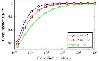
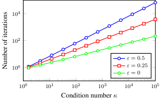
For fixed values of , , , , and , the feasibility of (11) is a semidefinite program with variables , , and . We perform a binary search over to find the minimal rate such that the linear matrix inequality in (11) is satisfied. The results are shown in Figure 1 for a wide range of condition numbers , for , and for several choices of . In Figure 2, we plot the values to show the number of iterations required to achieve a desired accuracy.
Note that when , the matrix is given by
and so the linear matrix inequality in (11) depends only on and not on and . Therefore, we will consider step sizes of this form (recall from (4) that ). The choice is common in the literature (Giselsson & Boyd, 2014), but requires the user to know the strong-convexity parameter . We also consider the choice , which produces worse guarantees, but does not require knowledge of .
One weakness of Theorem 6 is the fact that the rate we produce is not given as a function of . To use Theorem 6 as stated, we first specify the condition number (for example, ). Then we search for the minimal such that (11) is feasible. This produces an upper bound on the convergence rate of Algorithm 2 (for example, ). To remedy this problem, in Section 5, we demonstrate how Theorem 6 can be used to obtain the convergence rate of Algorithm 2 as a symbolic function of the step size and the over-relaxation parameter .
5 Symbolic Rates for Various and
In Section 4, we demonstrated how to use semidefinite programming to produce numerical convergence rates. That is, given a choice of algorithm parameters and the condition number , we could determine the convergence rate of Algorithm 2. In this section, we show how Theorem 6 can be used to prove symbolic convergence rates. That is, we describe the convergence rate of Algorithm 2 as a function of , , and . In Theorem 7, we prove the linear convergence of Algorithm 2 for all choices and , with . This result generalizes a number of results in the literature. As two examples, Giselsson & Boyd (2014) consider the case and Deng & Yin (2012) consider the case and .
The rate given in Theorem 7 is loose by a factor of four relative to the lower bound given in Theorem 8. However, weakening the rate by a constant factor eases the proof by making it easier to find a certificate for use in (11).
Theorem 7.
Proof.
We claim that for all sufficiently large , the linear matrix inequality in (11) is satisfied with the rate and with certificate
The matrix on the right hand side of (11) can be expressed as , where is a symmetric matrix whose last row and column consist of zeros. We wish to prove that is positive semidefinite for all sufficiently large . To do so, we consider the cases and separately, though the two cases will be nearly identical. First suppose that . In this case, the nonzero entries of are specified by
We show that each of the first three leading principal minors of is positive for sufficiently large . To understand the behavior of the leading principal minors, it suffices to look at their leading terms. For large , the first leading principal minor (which is simple ) is dominated by the term , which is positive. Similarly, the second leading principal minor is dominated by the term , which is positive. When , the third leading principal minor is dominated by the term , which is positive. When , the third leading principal minor is dominated by the term , which is positive. Since these leading coefficients are all positive, it follows that for all sufficiently large , the matrix is positive semidefinite.
Now suppose that . In this case, the nonzero entries of are specified by
As before, we show that each of the first three leading principal minors of is positive. For large , the first leading principal minor (which is simple ) is dominated by the term , which is positive. Similarly, the second leading principal minor is dominated by the term , which is positive. The third leading principal minor is dominated by the term , which is positive. Since these leading coefficients are all positive, it follows that for all sufficiently large , the matrix is positive semidefinite.
The result now follows from Theorem 6 by noting that has eigenvalues and . ∎
Note that since the matrix doesn’t depend on , the proof holds even when the step size changes at each iteration.
6 Lower Bounds
In this section, we probe the tightness of the upper bounds on the convergence rate of Algorithm 2 given by Theorem 6. The construction of the lower bound in this section is similar to a construction given in Ghadimi et al. (2015).
Let be a -dimensional symmetric positive-definite matrix whose largest and smallest eigenvalues are and respectively. Let be a quadratic and let for some . Let , , and . With these definitions, the optimization problem in (1) is solved by . The updates for Algorithm 2 are given by
| (13a) | ||||
| (13b) | ||||
| (13c) | ||||
Solving for in (13b) and substituting the result into (13c) gives . Then eliminating and from (13b) using (13a) and the fact that allows us to express the update rule purely in terms of as
Note that the eigenvalues of are given by
| (14) |
where is an eigenvalue of . We will use this setup to construct a lower bound on the worst-case convergence rate of Algorithm 2 in Theorem 8.
Theorem 8.
Proof.
First consider the case . Choosing and , from (14), we see that has eigenvalue
| (16) |
When initialized with as the eigenvector corresponding to this eigenvalue, Algorithm 2 will converge linearly with rate given exactly by (16), which is lower bounded by the expression in (15) when .
Now suppose that . Choosing and , after multiplying the numerator and denominator of (14) by , we see that has eigenvalue
| (17) |
When initialized with as the eigenvector corresponding to this eigenvalue, Algorithm 2 will converge linearly with rate given exactly by the left hand side of (17), which is lower bounded by the expression in (15) when . ∎
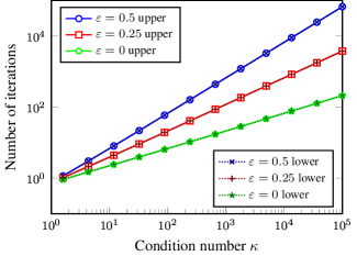
Figure 3 compares the lower bounds given by (16) with the upper bounds given by Theorem 6 for and for several choices of satisfying . The upper and lower bounds agree visually on the range of choices depicted, demonstrating the practical tightness of the upper bounds given by Theorem 6 for a large range of choices of parameter values.
7 Related Work
Several recent papers have studied the linear convergence of Algorithm 1 but do not extend to Algorithm 2. Deng & Yin (2012) prove a linear rate of convergence for ADMM in the strongly convex case. Iutzeler et al. (2014) prove the linear convergence of a specialization of ADMM to a class of distributed optimization problems under a local strong-convexity condition. Hong & Luo (2012) prove the linear convergence of a generalization of ADMM to a multiterm objective in the setting where each term can be decomposed as a strictly convex function and a polyhedral function. In particular, this result does not require strong convexity.
More generally, there are a number of results for operator splitting methods in the literature. Lions & Mercier (1979) and Eckstein & Ferris (1998) analyze the convergence of several operator splitting schemes. More recently, Patrinos et al. (2014a, b) prove the equivalence of forward-backward splitting and Douglas–Rachford splitting with a scaled version of the gradient method applied to unconstrained nonconvex surrogate functions (called the forward-backward envelope and the Douglas–Rachford envelope respectively). Goldstein et al. (2012) propose an accelerated version of ADMM in the spirit of Nesterov, and prove a convergence rate in the case where and are both strongly convex and is quadratic.
The theory of over-relaxed ADMM is more limited. Eckstein & Bertsekas (1992) prove the convergence of over-relaxed ADMM but do not give a rate. More recently, Davis & Yin (2014a, b) analyze the convergence rates of ADMM in a variety of settings. Giselsson & Boyd (2014) prove the linear convergence of Douglas–Rachford splitting in the strongly-convex setting. They use the fact that ADMM is Douglas–Rachford splitting applied to the dual problem (Eckstein & Bertsekas, 1992) to derive a linear convergence rate for over-relaxed ADMM with a specific choice of step size . Eckstein (1994) gives convergence results for several specializations of ADMM, and found that over-relaxation with empirically sped up convergence. Ghadimi et al. (2015) give some guidance on tuning over-relaxed ADMM in the quadratic case.
Unlike prior work, our framework requires no assumptions on the parameter choices in Algorithm 2. For example, Theorem 6 certifies the linear convergence of Algorithm 2 even for values . In our framework, certifying a convergence rate for an arbitrary choice of parameters amounts to checking the feasibility of a semidefinite program, which is essentially instantaneous, as opposed to formulating a proof.
8 Selecting Algorithm Parameters
In this section, we show how to use the results of Section 4 to select the parameters and in Algorithm 2 and we show the effect on a numerical example.
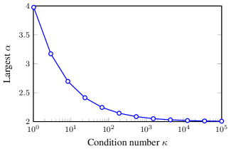
Recall that given a choice of parameters and and given the condition number , Theorem 6 gives an upper bound on the convergence rate of Algorithm 2. Therefore, one approach to parameter selection is to do a grid search over the space of parameters for the choice that minimizes the upper bound provided by Theorem 6. We demonstrate this approach numerically for a distributed Lasso problem, but first we demonstrate that the usual range of for the over-relaxation parameter is too limited, that more choices of lead to linear convergence. In Figure 4, we plot the largest value of found through binary search such that (11) is satisfied for some as a function of . Proof techniques in prior work do not extend as easily to values of . In our framework, we simply change some constants in a small semidefinite program.
8.1 Distributed Lasso
Following Deng & Yin (2012), we give a numerical demonstration with a distributed Lasso problem of the form
| minimize | |||
| subject to |
Each is a tall matrix with full column rank, and so the first term in the objective will be strongly convex and its gradient will be Lipschitz continuous. As in Deng & Yin (2012), we choose and . Each is generated by populating a matrix with independent standard normal entries and normalizing the columns. We generate each via , where is a sparse -dimensional vector with independent standard normal entries, and .
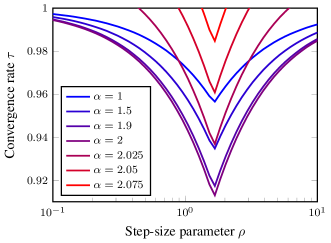
In Figure 5, we compute the upper bounds on the convergence rate given by Theorem 6 for a grid of values of and . Each line corresponds to a fixed choice of , and we plot only a subset of the values of to keep the plot manageable. We omit points corresponding to parameter values for which the linear matrix inequality in (11) was not feasible for any value of .
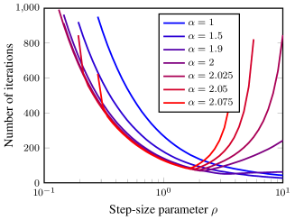
In Figure 6, we run Algorithm 2 for the same values of and . We then plot the number of iterations needed for to reach within of a precomputed reference solution. We plot lines corresponding to only a subset of the values of to keep the plot manageable, and we omit points corresponding to parameter values for which Algorithm 2 exceeded iterations. For the most part, the performance of Algorithm 2 as a function of closely tracked the performance predicted by the upper bounds in Figure 5. Notably, smaller values of seem more robust to poor choices of . The parameters suggested by our analysis perform close to the best of any parameter choices.
9 Discussion
We showed that a framework based on semidefinite programming can be used to prove convergence rates for the alternating direction method of multipliers and allows a unified treatment of the algorithm’s many variants, which arise through the introduction of additional parameters. We showed how to use this framework for establishing convergence rates, as in Theorem 6 and Theorem 7, and how to use this framework for parameter selection in practice, as in Section 8. The potential uses are numerous. This framework makes it straightforward to propose new algorithmic variants, for example, by introducing new parameters into Algorithm 2 and using Theorem 6 to see if various settings of these new parameters give rise to improved guarantees.
In the case that Assumption 3 does not hold, the most likely cause is that we lack the strong convexity of . One approach to handling this is to run Algorithm 2 on the modified function . By completing the square in the update, we see that this amounts to an extremely minor algorithmic modification (it only affects the update).
It should be clear that other operator splitting methods such as Douglas–Rachford splitting and forward-backward splitting can be cast in this framework and analyzed using the tools presented here.
Acknowledgments
This research is supported in part by NSF CISE Expeditions award CCF-1139158, LBNL award 7076018, DARPA XData award FA8750-12-2-0331, AFOSR award FA9550-12-1-0339, NASA grant NRA NNX12AM55A, ONR grants N00014-11-1-0688 and N00014-14-1-0024, US ARL and US ARO grant W911NF-11-1-0391, NSF awards CCF-1359814 and CCF-1217058, NSF grant DGE-1106400, a Sloan Research Fellowship, and gifts from Amazon Web Services, Google, SAP, The Thomas and Stacey Siebel Foundation, Adatao, Adobe, Apple, Blue Goji, Bosch, C3Energy, Cisco, Cray, Cloudera, EMC, Ericsson, Facebook, Guavus, Huawei, Informatica, Intel, Microsoft, NetApp, Pivotal, Samsung, Splunk, Virdata, VMware, and Yahoo!.
References
- Aslan et al. (2013) Aslan, Ö., Cheng, H., Zhang, X., and Schuurmans, D. Convex two-layer modeling. In Advances in Neural Information Processing Systems, pp. 2985–2993, 2013.
- Behmardi et al. (2014) Behmardi, B., Archambeau, C., and Bouchard, G. Overlapping trace norms in multi-view learning. arXiv preprint arXiv:1404.6163, 2014.
- Bioucas-Dias & Figueiredo (2010) Bioucas-Dias, J. M. and Figueiredo, M. A. T. Alternating direction algorithms for constrained sparse regression: application to hyperspectral unmixing. In Hyperspectral Image and Signal Processing: Evolution in Remote Sensing, pp. 1–4. IEEE, 2010.
- Bird (2014) Bird, S. Optimizing Resource Allocations for Dynamic Interactive Applications. PhD thesis, University of California, Berkeley, 2014.
- Boyd et al. (2011) Boyd, S., Parikh, N., Chu, E., Peleato, B., and Eckstein, J. Distributed optimization and statistical learning via the alternating direction method of multipliers. Foundations and Trends in Machine Learning, 3(1):1–122, 2011.
- Corless (1990) Corless, M. Guaranteed rates of exponential convergence for uncertain systems. Journal of Optimization Theory and Applications, 64(3):481–494, 1990.
- D’Alto & Corless (2013) D’Alto, L. and Corless, M. Incremental quadratic stability. Numerical Algebra, Control and Optimization, 3(1):175–201, 2013.
- Davis & Yin (2014a) Davis, D. and Yin, W. Convergence rate analysis of several splitting schemes. arXiv preprint arXiv:1406.4834, 2014a.
- Davis & Yin (2014b) Davis, D. and Yin, W. Convergence rates of relaxed Peaceman-Rachford and ADMM under regularity assumptions. arXiv preprint arXiv:1407.5210, 2014b.
- Deng & Yin (2012) Deng, W. and Yin, W. On the global and linear convergence of the generalized alternating direction method of multipliers. Technical report, DTIC Document, 2012.
- Eckstein (1994) Eckstein, J. Parallel alternating direction multiplier decomposition of convex programs. Journal of Optimization Theory and Applications, 80(1):39–62, 1994.
- Eckstein & Bertsekas (1992) Eckstein, J. and Bertsekas, D. P. On the Douglas–Rachford splitting method and the proximal point algorithm for maximal monotone operators. Mathematical Programming, 55(1-3):293–318, 1992.
- Eckstein & Ferris (1998) Eckstein, J. and Ferris, M. C. Operator-splitting methods for monotone affine variational inequalities, with a parallel application to optimal control. INFORMS Journal on Computing, 10(2):218–235, 1998.
- Forero et al. (2010) Forero, P. A., Cano, A., and Giannakis, G. B. Consensus-based distributed support vector machines. The Journal of Machine Learning Research, 11:1663–1707, 2010.
- Forouzan & Ihler (2013) Forouzan, S. and Ihler, A. Linear approximation to ADMM for MAP inference. In Asian Conference on Machine Learning, pp. 48–61, 2013.
- Gabay & Mercier (1976) Gabay, D. and Mercier, B. A dual algorithm for the solution of nonlinear variational problems via finite element approximation. Computers & Mathematics with Applications, 2(1):17–40, 1976.
- Ghadimi et al. (2015) Ghadimi, E., Teixeira, A., Shames, I., and Johansson, M. Optimal parameter selection for the alternating direction method of multipliers (ADMM): Quadratic problems. IEEE Transactions on Automatic Control, 60(3):644–658, 2015.
- Giselsson & Boyd (2014) Giselsson, P. and Boyd, S. Diagonal scaling in Douglas–Rachford splitting and ADMM. In IEEE Conference on Decision and Control, pp. 5033–5039, 2014.
- Glowinski & Marroco (1975) Glowinski, R. and Marroco, A. Sur l’approximation, par éléments finis d’ordre un, et la résolution, par pénalisation-dualité d’une classe de problèmes de Dirichlet non linéaires. ESAIM: Mathematical Modelling and Numerical Analysis-Modélisation Mathématique et Analyse Numérique, 9(R2):41–76, 1975.
- Goldstein et al. (2012) Goldstein, T., O’Donoghue, B., and Setzer, S. Fast alternating direction optimization methods. CAM report, pp. 12–35, 2012.
- Hong & Luo (2012) Hong, M. and Luo, Z.-Q. On the linear convergence of the alternating direction method of multipliers. arXiv preprint arXiv:1208.3922, 2012.
- Iutzeler et al. (2014) Iutzeler, F., Bianchi, P., Ciblat, Ph., and Hachem, W. Linear convergence rate for distributed optimization with the alternating direction method of multipliers. In IEEE Conference on Decision and Control, pp. 5046–5051, 2014.
- Lessard et al. (2014) Lessard, L., Recht, B., and Packard, A. Analysis and design of optimization algorithms via integral quadratic constraints. arXiv preprint arXiv:1408.3595, 2014.
- Li et al. (2014) Li, M., Andersen, D. G., Smola, A. J., and Yu, K. Communication efficient distributed machine learning with the parameter server. In Advances in Neural Information Processing Systems, pp. 19–27, 2014.
- Lions & Mercier (1979) Lions, P.-L. and Mercier, B. Splitting algorithms for the sum of two nonlinear operators. SIAM Journal on Numerical Analysis, 16(6):964–979, 1979.
- Meshi & Globerson (2011) Meshi, O. and Globerson, A. An alternating direction method for dual MAP LP relaxation. In Machine Learning and Knowledge Discovery in Databases, pp. 470–483. Springer, 2011.
- Patrinos et al. (2014a) Patrinos, P., Stella, L., and Bemporad, A. Douglas–Rachford splitting: complexity estimates and accelerated variants. In IEEE Conference on Decision and Control, pp. 4234–4239, 2014a.
- Patrinos et al. (2014b) Patrinos, P., Stella, L., and Bemporad, A. Forward-backward truncated Newton methods for large-scale convex composite optimization. arXiv preprint arXiv:1402.6655, 2014b.
- Romera-Paredes & Pontil (2013) Romera-Paredes, B. and Pontil, M. A new convex relaxation for tensor completion. In Advances in Neural Information Processing Systems, pp. 2967–2975, 2013.
- Sedghi et al. (2014) Sedghi, H., Anandkumar, A., and Jonckheere, E. Multi-step stochastic ADMM in high dimensions: Applications to sparse optimization and matrix decomposition. In Advances in Neural Information Processing Systems, pp. 2771–2779, 2014.
- Wahlberg et al. (2012) Wahlberg, B., Boyd, S., Annergren, M., and Wang, Y. An ADMM algorithm for a class of total variation regularized estimation problems. In IFAC Symposium on System Identification, pp. 83–88, 2012.
- Wang & Banerjee (2012) Wang, H. and Banerjee, A. Online alternating direction method. In International Conference on Machine Learning, pp. 1119–1126, 2012.
- Wang et al. (2013) Wang, H., Banerjee, A., Hsieh, C.-J., Ravikumar, P. K., and Dhillon, I. S. Large scale distributed sparse precision estimation. In Advances in Neural Information Processing Systems, pp. 584–592, 2013.
- Zhang et al. (2012) Zhang, C., Lee, H., and Shin, K. G. Efficient distributed linear classification algorithms via the alternating direction method of multipliers. In International Conference on Artificial Intelligence and Statistics, pp. 1398–1406, 2012.
- Zhang & Kwok (2014) Zhang, R. and Kwok, J. Asynchronous distributed ADMM for consensus optimization. In International Conference on Machine Learning, pp. 1701–1709, 2014.