Exploiting the Symmetries of P and S wave for BKμ+μ𝐵superscript𝐾superscript𝜇superscript𝜇B\to K^{*}\mu^{+}\mu^{-}

Lars Hofer and Joaquim Matias
Universitat Autònoma de Barcelona, 08193 Bellaterra, Barcelona
Abstract

After summarizing the current theoretical status of the four-body decay BK(Kπ)μ+μB\to K^{*}(\to K\pi)\mu^{+}\mu^{-}, we apply the formalism of spin-symmetries to the full angular distribution, including the S-wave part involving a broad scalar resonance K0subscriptsuperscript𝐾0K^{*}_{0}. While we recover in the P-wave sector the known relation between the angular observables Pi()superscriptsubscript𝑃𝑖P_{i}^{(\prime)}, we find in the S-wave sector two new relations connecting the coefficients of the S-wave angular distribution and reducing the number of independent S-wave observables from six to four. Included in the experimental data analysis, these relations can help to reduce the background from S-wave pollution. We further point out the discriminative power of the maximum of the angular observable P2subscript𝑃2P_{2} as a charm-loop insensitive probe of right-handed currents. Moreover, we show that in absence of right-handed currents the angular observables P4superscriptsubscript𝑃4P_{4}^{\prime} and P5superscriptsubscript𝑃5P_{5}^{\prime} fulfill the relation P4=βP5superscriptsubscript𝑃4𝛽superscriptsubscript𝑃5P_{4}^{\prime}=\beta P_{5}^{\prime} at the position where P2subscript𝑃2P_{2} reaches its maximum.

I Introduction

Rare B decays constitute one of the cornerstones in the search for physics beyond the Standard Model (SM). Among them, the semileptonic mode BK(Kπ)μ+μB\to K^{*}(\to K\pi)\mu^{+}\mu^{-} represents a particularly interesting channel as the measurement of the 4-body angular distribution provides a plethora of information which can be used to probe and discriminate different scenarios of New Physics (NP). In 2013, LHCb presented results of the measurement of an optimized set {Pi()}superscriptsubscript𝑃𝑖\{P_{i}^{(\prime)}\} of angular observables thefirst ; Becirevic:2011bp ; complete ; implications ; optimized based on 1 fb-1 data. These observables are constructed in such a way that, to leading order in the strong coupling constant αssubscript𝛼𝑠\alpha_{s} and in the large-recoil expansion, non-perturbative form factors cancel in the region of low squared invariant mass q2superscript𝑞2q^{2} of the dilepton pair, a unique and powerful feature in the hadronic environment.

Experimental data showed several interesting tensions with respect to SM expectations anomaly : Most striking is the 4σ4𝜎4\,\sigma anomaly111In Ref. explhcb this discrepancy is quoted as a 3.7σ3.7𝜎3.7\,\sigma tension between the experimental result and the 68.3% confidence level of the theoretical prediction, while we have quoted the tension between the experimental result and the theoretical central value. Note also that using the updated predictions impact for all observables, including parametric and form factor errors, factorizable power corrections together with an estimate of non-factorizable ones and charm-loop effects, the tensions with data, albeit slightly reduced, are still clearly present. encountered in the observable P5superscriptsubscript𝑃5P_{5}^{\prime} implications in the bin [4.3,8.68]4.38.68[4.3,8.68] GeV2. The observable P2subscript𝑃2P_{2} Becirevic:2011bp ; complete further displayed a 2.9σ2.9𝜎2.9\,\sigma deviation in the q2superscript𝑞2q^{2}-bin [2,4.3]24.3[2,4.3] GeV2. The position of its zero (q02=4.9±0.9superscriptsubscript𝑞02plus-or-minus4.90.9q_{0}^{2}=4.9\pm 0.9 GeV2), which is identical to the zero of the forward-backward asymmetry AFBsubscript𝐴FBA_{\rm FB}, is in agreement with the SM prediction q024similar-to-or-equalssuperscriptsubscript𝑞024q_{0}^{2}\simeq 4 GeV2 but allows for higher values. It is remarkable that all these deviations point to the same negative NP contribution C9NPsuperscriptsubscript𝐶9NPC_{9}^{\rm NP} to the Wilson coefficient of the semileptonic operator 𝒪9subscript𝒪9\mathcal{O}_{9}, possibly accompanied by a NP contribution C7NPsuperscriptsubscript𝐶7NPC_{7}^{\rm NP} to the Wilson coefficient of the magnetic operator 𝒪7subscript𝒪7\mathcal{O}_{7}. New Physics contributions to the Wilson coefficient C10subscript𝐶10C_{10}, and, in particular, to the coefficients C7,9,10superscriptsubscript𝐶7910C_{7,9,10}^{\prime} of the chirality-flipped operators are consistent with zero already at 1σ1𝜎1\,\sigma. The full pattern, first pointed out in Ref. anomaly and obtained using all available experimental bins in BKμ+μ𝐵superscript𝐾superscript𝜇superscript𝜇B\to K^{*}\mu^{+}\mu^{-} together with data on BKγ𝐵superscript𝐾𝛾B\to K^{*}\gamma, BXsγ𝐵subscript𝑋𝑠𝛾B\to X_{s}\gamma, BXsμ+μ𝐵subscript𝑋𝑠superscript𝜇superscript𝜇B\to X_{s}\mu^{+}\mu^{-} and Bsμ+μsubscript𝐵𝑠superscript𝜇superscript𝜇B_{s}\to\mu^{+}\mu^{-}, is given by the 1σ1𝜎1\,\sigma ranges

C9NPsuperscriptsubscript𝐶9NP\displaystyle C_{9}^{\rm NP} \displaystyle\in [1.6,0.9],C7NP[0.05,0.01],C10NP[0.4,1.0],formulae-sequence1.60.9superscriptsubscript𝐶7NP0.050.01superscriptsubscript𝐶10NP0.41.0\displaystyle[-1.6,-0.9],\quad\quad\quad\;\,C_{7}^{\rm NP}\in[-0.05,-0.01],\quad\quad\quad C_{10}^{\rm NP}\in[-0.4,1.0],
C9NPsuperscriptsubscript𝐶9NP\displaystyle C_{9}^{\prime\rm NP} \displaystyle\in [0.2,0.8],C7NP[0.04,0.02],C10NP[0.4,0.4],formulae-sequence0.20.8superscriptsubscript𝐶7NP0.040.02superscriptsubscript𝐶10NP0.40.4\displaystyle[-0.2,0.8],\quad\quad\quad\quad C_{7}^{\prime\rm NP}\in[-0.04,0.02],\quad\quad\quad\;\;C_{10}^{\prime\rm NP}\in[-0.4,0.4], (1)

where the mild preference for a positive C10NPsuperscriptsubscript𝐶10NPC_{10}^{\rm NP} is mainly driven by Bsμ+μsubscript𝐵𝑠superscript𝜇superscript𝜇B_{s}\to\mu^{+}\mu^{-} data.

The large negative NP contribution to C9subscript𝐶9C_{9} was independently confirmed later on by other groups, using different observables Sisubscript𝑆𝑖S_{i} buras ; straub (relying on the single large-recoil bin [1,6] GeV2 and low recoil data), different statistical approaches bayesian or form factor input from lattice meinelwingate . Although it had been shown in Refs. anomaly ; proceedvip that a large C9NP+C9<0superscriptsubscript𝐶9NPsuperscriptsubscript𝐶90C_{9}^{\rm NP}+C_{9}^{\prime}<0 was preferred in order to explain the P5superscriptsubscript𝑃5P_{5}^{\prime} anomaly, the possibility of a substantial positive C9superscriptsubscript𝐶9C_{9}^{\prime} enforcing C9NP+C90similar-tosuperscriptsubscript𝐶9NPsuperscriptsubscript𝐶90C_{9}^{\rm NP}+C_{9}^{\prime}\sim 0 was discussed in Refs. straub ; hiller , driven mainly by the 1 fb-1 data bkpp1fb on the charged B𝐵B decay B+K+μ+μsuperscript𝐵superscript𝐾superscript𝜇superscript𝜇B^{+}\to K^{+}\mu^{+}\mu^{-} in the region of low hadronic recoil. The situation has become more coherent recently as the latest 3 fb-1 data on B+K+μ+μsuperscript𝐵superscript𝐾superscript𝜇superscript𝜇B^{+}\to K^{+}\mu^{+}\mu^{-} and B0K0μ+μsuperscript𝐵0superscript𝐾0superscript𝜇superscript𝜇B^{0}\to K^{0}\mu^{+}\mu^{-} provided by LHCb bkpp3fb is also in good agreement with the solution C9NP+C9<0superscriptsubscript𝐶9𝑁𝑃superscriptsubscript𝐶90C_{9}^{NP}+C_{9}^{\prime}<0 anomaly , both in the region of large as well as low hadronic recoil inprepa ; wingate . The three modes thus seem to point to a consistent overall picture of NP in agreement with the pattern given by Eq. (I). Moreover, under the assumption that NP affects only muons but not electrons, also the 2.6σ2.6𝜎2.6\,\sigma deviation measured by LHCb lhcbrk in the observable

RK=Br(B+K+μ+μ)Br(B+K+e+e)subscript𝑅𝐾B𝑟superscript𝐵superscript𝐾superscript𝜇superscript𝜇B𝑟superscript𝐵superscript𝐾superscript𝑒superscript𝑒R_{K}=\frac{{\text{B}r}(B^{+}\to K^{+}\mu^{+}\mu^{-})}{{\text{B}r}(B^{+}\to K^{+}e^{+}e^{-})} (2)

can be explained within the same scenario ghosh ; Hurth:2014vma ; straub2 . In order to be able to draw solid conclusions and to see how this pattern evolves, it will be crucial to know the 3 fb-1 data on the observables Pi()superscriptsubscript𝑃𝑖P_{i}^{({\prime})} in BKμ+μ𝐵superscript𝐾superscript𝜇superscript𝜇B\to K^{*}\mu^{+}\mu^{-}.

In parallel, the question has been raised if the observed discrepancies between data and SM predictions could be attributed to non-perturbative QCD effects jaeger , even though hadronic form factors enter optimized observables Pi()superscriptsubscript𝑃𝑖P_{i}^{(\prime)} only at order αssubscript𝛼𝑠\alpha_{s} or through corrections breaking the large-recoil symmetries (factorisable power corrections). There exist two different approaches to account for factorisable power corrections: they can either be calculated (under certain modelling assumptions) within a non-perturbative framework like light-cone sum-rules (LCSR) straub ; StraubZwicky , or they can be estimated exclusively on the basis of dimensional arguments and fundamental model-independent relations jaeger ; impact ; jaeger2 . While the first method with full correlations among the form factors is suitable in order to extract the maximal information from a particular non-perturbative calculation, the second option in which correlations are included via large-recoil symmetry relations reduces the dependence on non-perturbative input to a minimum. The two approaches are thus complementary and, because the large-recoil symmetries are expected to be the dominant source of correlations, they should give similar results. Indeed, the resulting uncertainties obtained with the first method in Ref. straub and with the second method in Ref. impact are of the same order of magnitude (see also Ref. proc ). Both these analyses find hadronic uncertainties from form factors to be under control222Refs. jaeger ; jaeger2 , on the other hand, quote much larger uncertainties. One of the reasons for that has been identified in Ref. impact : the decomposition of a form factor into a leading-order part and a 𝒪(Λ/mb)𝒪Λsubscript𝑚𝑏\mathcal{O}(\Lambda/m_{b}) power correction is not unique but (as in any fixed-order calculation) introduces a scheme dependence of observables at neglected higher orders in Λ/mbΛsubscript𝑚𝑏\Lambda/m_{b}. As the observables are effectively calculated at leading order (𝒪(Λ/mb)𝒪Λsubscript𝑚𝑏\mathcal{O}(\Lambda/m_{b}) effects are not calculated but only estimated), they exhibit a scheme dependence at 𝒪(Λ/mb)𝒪Λsubscript𝑚𝑏\mathcal{O}(\Lambda/m_{b}) implying a 100%similar-toabsentpercent100\sim 100\% scheme dependence of power corrections. In order to ensure predictivity of the method, it is hence crucial to exploit the freedom of choosing a scheme to minimize the impact of the unknown power corrections on the relevant observables (in the same way as in a fixed-order calculation in quantum field theory the renormalization scheme is chosen such that neglected higher orders do not spoil the perturbative expansion). It was demonstrated in Ref. impact that the sensitivity to factorizable power corrections of the key observables like P5superscriptsubscript𝑃5P_{5}^{\prime} is significantly reduced if a different scheme is chosen than the one employed in Refs. jaeger ; jaeger2 ..

As a different explanation of the anomaly, the possibility of a large non-perturbative charm-loop contribution has been proposed zwicky , requiring a huge correction with respect to theory predictions within the factorization approximation. The discussion in Ref. zwicky relies on two model-dependent assumptions: First that the resonance structure obtained from a fit to high-q2superscript𝑞2q^{2} data on the scalar mode B+K+μ+μsuperscript𝐵superscript𝐾superscript𝜇superscript𝜇B^{+}\to K^{+}\mu^{+}\mu^{-} can directly be transferred to the vector mode BKμ+μ𝐵superscript𝐾superscript𝜇superscript𝜇B\to K^{*}\mu^{+}\mu^{-}, and second that it can be extrapolated to low values of q2superscript𝑞2q^{2}. The only existing calculation khodjamirian seems to be in contradiction with the low-q2superscript𝑞2q^{2} scenarios of BKμ+μ𝐵superscript𝐾superscript𝜇superscript𝜇B\to K^{*}\mu^{+}\mu^{-} obtained with this ansatz in Ref. zwicky as it finds a much smaller size for the charm loop and, moreover, the opposite sign for its contribution in B+K+μ+μsuperscript𝐵superscript𝐾superscript𝜇superscript𝜇B^{+}\to K^{+}\mu^{+}\mu^{-} as compared to BKμ+μ+𝐵superscript𝐾superscript𝜇superscript𝜇B\to K^{*}\mu^{+}\mu^{+} (contrary to the assumption in Ref. zwicky ). Furthermore, if the 2.6σ𝜎\sigma deviation in the observable RKsubscript𝑅𝐾R_{K} persists, it poses a serious problem for the charm-loop or any other low-energy QCD explanation which cannot generate effects violating lepton-flavor universality. Also the observable P2subscript𝑃2P_{2} in BKμ+μ+𝐵superscript𝐾superscript𝜇superscript𝜇B\to K^{*}\mu^{+}\mu^{+} can be instrumental in testing the charm-loop hypothesis proposed in Ref. zwicky (see also proc ).

While the polluting effects from non-perturbative QCD have been studied in detail in the literature, less attention has been paid to the so-called S-wave pollution, generated by the background decay BK0(Kπ)μ+μB\to K^{*}_{0}(\to K\pi)\mu^{+}\mu^{-} where K0subscriptsuperscript𝐾0K^{*}_{0} is a broad scalar resonance. In Ref. becirevicswave a detailed and complete calculation of the S-wave background was performed and it was concluded that any observable will unavoidably suffer from its pollution. While this conclusion is correct in the case of uniangular distributions, it does not apply to full or folded distributions where the P- and the S-wave parts can be separated according to their different angular dependence. As shown in Ref. swave , S-wave pollution can be avoided for the Pi()superscriptsubscript𝑃𝑖P_{i}^{(\prime)} observables if folded distributions are used instead of uniangular ones. A discussion of the experimental implications of the S-wave contribution was presented in Ref. ulrikswave (see also Ref. julich ).

Experimental analyses of BKμ+μ𝐵superscript𝐾superscript𝜇superscript𝜇B\to K^{*}\mu^{+}\mu^{-} rely on theoretical information regarding the S-wave background. To this end, a set of model-independent bounds on the coefficients of the S-wave part of the angular distribution was presented in Ref. optimized , derived from application of the Cauchy-Schwarz inequality. On the other hand, it was shown in Refs. ulrik1 ; complete that the coefficients of the P-wave part are not independent parameters but that they are correlated through the spin-symmetry of the angular distribution. In this work we transfer this idea to the S-wave sector. We derive two relations which effectively reduce the number of free coefficients of the S-wave distribution from six to four. It is expected that the inclusion of these relations into the data analysis can help to further improve the background estimation. We illustrate the effect of the correlations for the ratio of the S-wave observables AS4superscriptsubscript𝐴𝑆4A_{S}^{4} and AS5superscriptsubscript𝐴𝑆5A_{S}^{5} and study implications at the position q2=q12superscript𝑞2superscriptsubscript𝑞12q^{2}=q_{1}^{2} of the maximum of the observable P2subscript𝑃2P_{2}. Moreover, we point out a relation between P4superscriptsubscript𝑃4P_{4}^{\prime} and P5superscriptsubscript𝑃5P_{5}^{\prime} at q2=q12superscript𝑞2superscriptsubscript𝑞12q^{2}=q_{1}^{2} and suggest to use the maximum of P2subscript𝑃2P_{2} as a golden observable to probe right-handed currents (for an explicit model generating right-handed currents see e.g. Ref. lunghi ).

The outline of this paper is the following: In Sec. II we discuss the spin-symmetry of the differential BKμ+μ𝐵superscript𝐾superscript𝜇superscript𝜇B\to K^{*}\mu^{+}\mu^{-} decay rate and determine the number of independent observables in the P- and in the S-wave sector. In Sec. III we derive the resulting symmetry relations. Their phenomenological consequences are discussed in Sec. IV. First, we study the discriminating power of the maximum of P2subscript𝑃2P_{2} as a test for right-handed currents, then we determine a relation between P4superscriptsubscript𝑃4P_{4}^{\prime} and P5superscriptsubscript𝑃5P_{5}^{\prime} at the position of the maximum of P2subscript𝑃2P_{2}, and finally we investigate constraints on the S-wave observables AS(i)superscriptsubscript𝐴𝑆𝑖A_{S}^{(i)} and derive simple relations among them at the position of the maximum and the zero of P2subscript𝑃2P_{2}. Sec. V contains our conclusions. In Appendix A we present an explicit example of how to use the freedom introduced by the symmetries to fix a possible convention for the amplitudes, while Appendix B contains details of the derivation of the bound on ASsubscript𝐴𝑆A_{S}.

II Spin symmetry of the differential decay rate

The differential decay rate of the full four-body decay BKπ+𝐵𝐾𝜋superscriptsuperscriptB\to K\pi\ell^{+}\ell^{-} receives contributions from the P-wave decay BK(Kπ)+B\to K^{*}(\to K\pi)\ell^{+}\ell^{-} as well as from the S-wave decay BK0(Kπ)+B\to K_{0}^{*}(\to K\pi)\ell^{+}\ell^{-} with K0superscriptsubscript𝐾0K_{0}^{*} being a broad scalar resonance. It can thus be decomposed into a P-wave and an S-wave part,

d5Γdq2dmKπ2dcosθKdcosθdϕ=WP+WS,superscript𝑑5Γ𝑑superscript𝑞2𝑑superscriptsubscript𝑚𝐾𝜋2𝑑subscript𝜃𝐾𝑑subscript𝜃𝑑italic-ϕsubscript𝑊𝑃subscript𝑊𝑆\frac{d^{5}\Gamma}{dq^{2}\,dm_{K\pi}^{2}\,d\!\cos\theta_{K}\,d\!\cos\theta_{\ell}\,d\phi}\,=\,W_{P}\,+\,W_{S}, (3)

with WPsubscript𝑊𝑃W_{P} containing the pure P-wave contribution and WSsubscript𝑊𝑆W_{S} containing the contributions from pure S-wave exchange as well as from S-P interference. Here, q2superscript𝑞2q^{2} denotes the square of the invariant mass of the lepton pair and mKπsubscript𝑚𝐾𝜋m_{K\pi} the invariant mass of the Kπ𝐾𝜋K\pi system. Further, θsubscript𝜃\theta_{\ell}, θKsubscript𝜃𝐾\theta_{K} are the angles describing the relative directions of flight of the final-state particles, while ϕitalic-ϕ\phi is the angle between the dilepton and the dimeson plane (see Ref. ulrik1 for exact definitions). Angular momentum conservation dictates the dependence of WPsubscript𝑊𝑃W_{P} and WSsubscript𝑊𝑆W_{S} on θsubscript𝜃\theta_{\ell}, θKsubscript𝜃𝐾\theta_{K}, ϕitalic-ϕ\phi to be

WPsubscript𝑊𝑃\displaystyle W_{P} =\displaystyle= 932π[J1ssin2θK+J1ccos2θK+(J2ssin2θK+J2ccos2θK)cos2θl\displaystyle\frac{9}{32\pi}\left[J_{1s}\sin^{2}\theta_{K}+J_{1c}\cos^{2}\theta_{K}+(J_{2s}\sin^{2}\theta_{K}+J_{2c}\cos^{2}\theta_{K})\cos 2\theta_{l}\right. (4)
+J3sin2θKsin2θlcos2ϕ+J4sin2θKsin2θlcosϕ+J5sin2θKsinθlcosϕsubscript𝐽3superscript2subscript𝜃𝐾superscript2subscript𝜃𝑙2italic-ϕsubscript𝐽42subscript𝜃𝐾2subscript𝜃𝑙italic-ϕsubscript𝐽52subscript𝜃𝐾subscript𝜃𝑙italic-ϕ\displaystyle\hskip 28.45274pt+J_{3}\sin^{2}\theta_{K}\sin^{2}\theta_{l}\cos 2\phi+J_{4}\sin 2\theta_{K}\sin 2\theta_{l}\cos\phi+J_{5}\sin 2\theta_{K}\sin\theta_{l}\cos\phi
+(J6ssin2θK+J6ccos2θK)cosθl+J7sin2θKsinθlsinϕ+J8sin2θKsin2θlsinϕsubscript𝐽6𝑠superscript2subscript𝜃𝐾subscript𝐽6𝑐superscript2subscript𝜃𝐾subscript𝜃𝑙subscript𝐽72subscript𝜃𝐾subscript𝜃𝑙italic-ϕsubscript𝐽82subscript𝜃𝐾2subscript𝜃𝑙italic-ϕ\displaystyle\hskip 28.45274pt+(J_{6s}\sin^{2}\theta_{K}+{J_{6c}\cos^{2}\theta_{K}})\cos\theta_{l}+J_{7}\sin 2\theta_{K}\sin\theta_{l}\sin\phi+J_{8}\sin 2\theta_{K}\sin 2\theta_{l}\sin\phi
+J9sin2θKsin2θlsin2ϕ]\displaystyle\hskip 28.45274pt\left.+J_{9}\sin^{2}\theta_{K}\sin^{2}\theta_{l}\sin 2\phi\right]

and

WSsubscript𝑊𝑆\displaystyle W_{S} =\displaystyle= 14π[J~1ac+J~1bccosθK+(J~2ac+J~2bccosθK)cos2θ+J~4sinθKsin2θcosϕ\displaystyle\frac{1}{4\pi}\left[{\tilde{J}}_{1a}^{c}+{\tilde{J}}_{1b}^{c}\cos\theta_{K}+({\tilde{J}}_{2a}^{c}+{\tilde{J}}_{2b}^{c}\cos\theta_{K})\cos 2\theta_{\ell}+{\tilde{J}}_{4}\sin\theta_{K}\sin 2\theta_{\ell}\cos\phi\right. (5)
+J~5sinθKsinθcosϕ+J~7sinθKsinθsinϕ+J~8sinθKsin2θsinϕ].\displaystyle\left.\hskip 19.91684pt+{\tilde{J}}_{5}\sin\theta_{K}\sin\theta_{\ell}\cos\phi+{\tilde{J}}_{7}\sin\theta_{K}\sin\theta_{\ell}\sin\phi+{\tilde{J}}_{8}\sin\theta_{K}\sin 2\theta_{\ell}\sin\phi\right].

The coefficients Jisubscript𝐽𝑖J_{i} and J~isubscript~𝐽𝑖\tilde{J}_{i} are functions of q2superscript𝑞2q^{2} and mKπ2superscriptsubscript𝑚𝐾𝜋2m_{K\pi}^{2}.

If not explicitly stated otherwise, we will neglect lepton masses in the following. Then, the decays BK+𝐵superscript𝐾superscriptsuperscriptB\to K^{*}\ell^{+}\ell^{-} and BK0+𝐵superscriptsubscript𝐾0superscriptsuperscriptB\to K_{0}^{*}\ell^{+}\ell^{-} are described by six complex amplitudes A,,0L,RA_{\|,\bot,0}^{L,R} and two complex amplitudes A0L,Rsuperscriptsubscript𝐴0𝐿𝑅A_{0}^{\prime L,R}, respectively, where the upper index L,R𝐿𝑅L,R refers to the chirality of the outgoing lepton current, while in the case of the P-wave the lower index ,,0\|,\bot,0 indicates the helicity of the Ksuperscript𝐾K^{*}-meson333In the case of non-vanishing lepton masses and of scalar operators coupling to the lepton pair, two additional amplitudes Atsubscript𝐴𝑡A_{t} and ASsubscript𝐴𝑆A_{S} have to be included.. These amplitudes are multiplied by a Breit-Wigner propagator BWi(mKπ2)𝐵subscript𝑊𝑖superscriptsubscript𝑚𝐾𝜋2BW_{i}(m_{K\pi}^{2}) with i=K,K0𝑖superscript𝐾subscriptsuperscript𝐾0i=K^{*},K^{*}_{0} describing the propagation of the Ksuperscript𝐾K^{*} and K0superscriptsubscript𝐾0K_{0}^{*} meson, respectively. For the exact form of the Breit-Wigner functions BWi(mKπ2)𝐵subscript𝑊𝑖superscriptsubscript𝑚𝐾𝜋2BW_{i}(m_{K\pi}^{2}) we refer to Ref. becirevicswave .

Since the final state is summed over the spins of the leptons, the obervables Jisubscript𝐽𝑖J_{i} and J~isubscript~𝐽𝑖\tilde{J}_{i} are exclusively described in terms of spin-summed squared amplitudes of the form AiLAjL±AiRAjRplus-or-minussuperscriptsubscript𝐴𝑖𝐿superscriptsubscript𝐴𝑗𝐿superscriptsubscript𝐴𝑖𝑅superscriptsubscript𝐴𝑗𝑅A_{i}^{L*}A_{j}^{L}\pm A_{i}^{R*}A_{j}^{R} 444Interferences of different Ksuperscript𝐾K^{*} and K0superscriptsubscript𝐾0K_{0}^{*} helicities ij𝑖𝑗i\not=j contribute, as these particles only appear as unobserved intermediate states.. This pattern suggests to combine left- and right-handed amplitudes to two-component complex vectors:

n=(ALBWPARBWP),n=(ALBWPARBWP),n0=(A0LBWPA0RBWP),nS=(A0LBWSA0RBWS).formulae-sequencesubscript𝑛binomialsuperscriptsubscript𝐴𝐿𝐵subscript𝑊𝑃superscriptsubscript𝐴𝑅𝐵superscriptsubscript𝑊𝑃formulae-sequencesubscript𝑛bottombinomialsuperscriptsubscript𝐴bottom𝐿𝐵subscript𝑊𝑃superscriptsubscript𝐴bottom𝑅𝐵superscriptsubscript𝑊𝑃formulae-sequencesubscript𝑛0binomialsuperscriptsubscript𝐴0𝐿𝐵subscript𝑊𝑃superscriptsubscript𝐴0𝑅𝐵superscriptsubscript𝑊𝑃subscript𝑛𝑆binomialsuperscriptsubscript𝐴0𝐿𝐵subscript𝑊𝑆superscriptsubscript𝐴0𝑅𝐵superscriptsubscript𝑊𝑆n_{\|}=\binom{A_{\|}^{L}BW_{P}}{A_{\|}^{R*}BW_{P}^{*}}\ ,\quad n_{\bot}=\binom{A_{\bot}^{L}BW_{P}}{-A_{\bot}^{R*}BW_{P}^{*}}\ ,\quad n_{0}=\binom{A_{0}^{L}BW_{P}}{A_{0}^{R*}BW_{P}^{*}}\ ,\quad n_{S}=\binom{A_{0}^{\prime L}BW_{S}}{A_{0}^{\prime R*}BW_{S}^{*}}\ . (6)

Using this notation, the observables Jisubscript𝐽𝑖J_{i} and J~isubscript~𝐽𝑖\tilde{J}_{i} can be expressed in terms of scalar products ninjsuperscriptsubscript𝑛𝑖subscript𝑛𝑗n_{i}^{\dagger}n_{j} of these vectors. Neglecting lepton masses and presence of scalars we find

J1ssubscript𝐽1𝑠\displaystyle J_{1s} =\displaystyle= 34(|n|2+|n|2),J1c=|n0|2,J2s=14(|n|2+|n|2),formulae-sequence34superscriptsubscript𝑛bottom2superscriptsubscript𝑛2subscript𝐽1𝑐superscriptsubscript𝑛02subscript𝐽2𝑠14superscriptsubscript𝑛bottom2superscriptsubscript𝑛2\displaystyle\frac{3}{4}\left(|n_{\bot}|^{2}+|n_{\|}|^{2}\right),\hskip 25.6073ptJ_{1c}\,=\,|n_{0}|^{2}\,,\hskip 85.35826ptJ_{2s}\,=\,\frac{1}{4}\left(|n_{\bot}|^{2}+|n_{\|}|^{2}\right)\,,
J2csubscript𝐽2𝑐\displaystyle J_{2c} =\displaystyle= |n0|2,J3=12(|n|2|n|2),J4=12Re(n0n),formulae-sequencesuperscriptsubscript𝑛02subscript𝐽312superscriptsubscript𝑛bottom2superscriptsubscript𝑛2subscript𝐽412Resuperscriptsubscript𝑛0subscript𝑛\displaystyle-|n_{0}|^{2}\,,\hskip 81.09052ptJ_{3}\,=\,\frac{1}{2}\left(|n_{\bot}|^{2}-|n_{\|}|^{2}\right)\,,\hskip 25.6073ptJ_{4}\,=\,\frac{1}{\sqrt{2}}\text{Re}(n_{0}^{\dagger}\,n_{\|})\,,
J5subscript𝐽5\displaystyle J_{5} =\displaystyle= 2Re(n0n),J6s= 2Re(nn),J7=2Im(n0n),formulae-sequence2Resuperscriptsubscript𝑛0subscript𝑛bottomsubscript𝐽6𝑠2Resuperscriptsubscript𝑛bottomsubscript𝑛subscript𝐽72Imsuperscriptsubscript𝑛0subscript𝑛\displaystyle\sqrt{2}\,\text{Re}(n_{0}^{\dagger}\,n_{\bot})\,,\hskip 41.25641ptJ_{6s}\,=\,2\,\text{Re}(n_{\bot}^{\dagger}\,n_{\|})\,,\hskip 52.63777ptJ_{7}\,=\,-\sqrt{2}\,\text{Im}(n_{0}^{\dagger}\,n_{\|})\,,
J8subscript𝐽8\displaystyle J_{8} =\displaystyle\,=\, 12Im(n0n),J9=Im(nn),J6c= 0,formulae-sequence12Imsuperscriptsubscript𝑛0subscript𝑛bottomsubscript𝐽9Imsuperscriptsubscript𝑛bottomsubscript𝑛subscript𝐽6𝑐 0\displaystyle-\frac{1}{\sqrt{2}}\text{Im}(n_{0}^{\dagger}\,n_{\bot})\,,\hskip 35.56593ptJ_{9}\,=\,-\text{Im}(n_{\bot}^{\dagger}\,n_{\|})\,,\hskip 46.94687ptJ_{6c}\,=\,0\,, (7)

and

J~1ac=J~2acsuperscriptsubscript~𝐽1𝑎𝑐superscriptsubscript~𝐽2𝑎𝑐\displaystyle{\tilde{J}_{1a}^{c}}=-{\tilde{J}_{2a}^{c}} =\displaystyle= 38(|A0L|2+|A0R|2)|BWS|2=38|nS|2,38superscriptsuperscriptsubscript𝐴0𝐿2superscriptsuperscriptsubscript𝐴0𝑅2superscript𝐵subscript𝑊𝑆238superscriptsubscript𝑛𝑆2\displaystyle\frac{3}{8}(|A_{0}^{\prime L}|^{2}+|A_{0}^{\prime R}|^{2})|BW_{S}|^{2}=\frac{3}{8}|n_{S}|^{2},
J~1bc=J~2bcsuperscriptsubscript~𝐽1𝑏𝑐superscriptsubscript~𝐽2𝑏𝑐\displaystyle{\tilde{J}_{1b}^{c}}=-{\tilde{J}_{2b}^{c}} =\displaystyle= 343Re[(A0LA0L+A0RA0R)BWSBWP]=343Re(nSn0),343Redelimited-[]superscriptsubscript𝐴0𝐿superscriptsubscript𝐴0𝐿superscriptsubscript𝐴0𝑅superscriptsubscript𝐴0𝑅𝐵subscript𝑊𝑆𝐵superscriptsubscript𝑊𝑃343Resuperscriptsubscript𝑛𝑆subscript𝑛0\displaystyle\frac{3}{4}\sqrt{3}{\rm Re}\left[(A_{0}^{\prime L}A_{0}^{L*}+A_{0}^{\prime R}A_{0}^{R*})BW_{S}BW_{P}^{*}\right]=\frac{3}{4}\sqrt{3}{\rm Re}(n_{S}^{\dagger}\,n_{0}),
J~4subscript~𝐽4\displaystyle{\tilde{J}_{4}} =\displaystyle= 3432Re[(A0LAL+A0RAR)BWSBWP]=3432Re(nSn),3432Redelimited-[]superscriptsubscript𝐴0𝐿superscriptsubscript𝐴𝐿superscriptsubscript𝐴0𝑅superscriptsubscript𝐴𝑅𝐵subscript𝑊𝑆𝐵superscriptsubscript𝑊𝑃3432Resuperscriptsubscript𝑛𝑆subscript𝑛\displaystyle\frac{3}{4}\sqrt{\frac{3}{2}}{\rm Re}\left[(A_{0}^{\prime L}A_{\|}^{L*}+A_{0}^{\prime R}A_{\|}^{R*})BW_{S}BW_{P}^{*}\right]=\frac{3}{4}\sqrt{\frac{3}{2}}{\rm Re}(n_{S}^{\dagger}\,n_{\|}),
J~5subscript~𝐽5\displaystyle{\tilde{J}_{5}} =\displaystyle= 3232Re[(A0LALA0RAR)BWSBWP]=3232Re(nSn),3232Redelimited-[]superscriptsubscript𝐴0𝐿superscriptsubscript𝐴perpendicular-to𝐿superscriptsubscript𝐴0𝑅superscriptsubscript𝐴perpendicular-to𝑅𝐵subscript𝑊𝑆𝐵superscriptsubscript𝑊𝑃3232Resuperscriptsubscript𝑛𝑆subscript𝑛perpendicular-to\displaystyle\frac{3}{2}\sqrt{\frac{3}{2}}{\rm Re}\left[(A_{0}^{\prime L}A_{\perp}^{L*}-A_{0}^{\prime R}A_{\perp}^{R*})BW_{S}BW_{P}^{*}\right]=\frac{3}{2}\sqrt{\frac{3}{2}}{\rm Re}(n_{S}^{\dagger}\,n_{\perp}),
J~7subscript~𝐽7\displaystyle{\tilde{J}_{7}} =\displaystyle= 3232Im[(A0LALA0RAR)BWSBWP]=3232Im(nnS),3232Imdelimited-[]superscriptsubscript𝐴0𝐿superscriptsubscript𝐴𝐿superscriptsubscript𝐴0𝑅superscriptsubscript𝐴𝑅𝐵subscript𝑊𝑆𝐵superscriptsubscript𝑊𝑃3232Imsuperscriptsubscript𝑛subscript𝑛𝑆\displaystyle\frac{3}{2}\sqrt{\frac{3}{2}}{\rm Im}\left[(A_{0}^{\prime L}A_{\|}^{L*}-A_{0}^{\prime R}A_{\|}^{R*})BW_{S}BW_{P}^{*}\right]=\frac{3}{2}\sqrt{\frac{3}{2}}{\rm Im}(n_{\|}^{\dagger}\,n_{S}),
J~8subscript~𝐽8\displaystyle{\tilde{J}_{8}} =\displaystyle= 3432Im[(A0LAL+A0RAR)BWSBWP]=3432Im(nnS).3432Imdelimited-[]superscriptsubscript𝐴0𝐿superscriptsubscript𝐴perpendicular-to𝐿superscriptsubscript𝐴0𝑅superscriptsubscript𝐴perpendicular-to𝑅𝐵subscript𝑊𝑆𝐵superscriptsubscript𝑊𝑃3432Imsuperscriptsubscript𝑛perpendicular-tosubscript𝑛𝑆\displaystyle\frac{3}{4}\sqrt{\frac{3}{2}}{\rm Im}\left[(A_{0}^{\prime L}A_{\perp}^{L*}+A_{0}^{\prime R}A_{\perp}^{R*})BW_{S}BW_{P}^{*}\right]=\frac{3}{4}\sqrt{\frac{3}{2}}{\rm Im}(n_{\perp}^{\dagger}n_{S}). (8)

The fact that the Jisubscript𝐽𝑖J_{i} and J~isubscript~𝐽𝑖\tilde{J}_{i} observables involve a sum over the spins of the leptons implies that they are not sensitive to the full information contained in the helicity amplitudes A,,0L,RA_{\|,\bot,0}^{L,R}, A0L,Rsuperscriptsubscript𝐴0𝐿𝑅A_{0}^{\prime L,R}. This can be easily seen from the notation in terms of the vectors nisubscript𝑛𝑖n_{i}. As the Jisubscript𝐽𝑖J_{i} and J~isubscript~𝐽𝑖\tilde{J}_{i} observables are scalar products of the nisubscript𝑛𝑖n_{i}, they are invariant under a U(2)𝑈2U(2) rotation of these vectors. It is thus impossible to fully reconstruct the amplitudes from the Ji,J~isubscript𝐽𝑖subscript~𝐽𝑖J_{i},\tilde{J}_{i} observables alone. If one wishes to extract the A,,0L,RA_{\|,\bot,0}^{L,R}, A0L,Rsuperscriptsubscript𝐴0𝐿𝑅A_{0}^{\prime L,R} from experiment, it is mandatory to fix a convention which resolves the ambiguity related to the U(2)𝑈2U(2) symmetry. A possible choice is presented in Appendix A.

The number of independent observables that can be constructed from nAsubscript𝑛𝐴n_{A} complex amplitudes is given by 2nA2subscript𝑛𝐴2n_{A}. In presence of a symmetry S𝑆S with ngensubscript𝑛genn_{\rm gen} generators, there exist

nObs= 2nAngensubscript𝑛Obs2subscript𝑛𝐴subscript𝑛genn_{\rm Obs}\,=\,2n_{A}-n_{\rm gen} (9)

independent observables which respect the symmetry S𝑆S. The U(2)𝑈2U(2) spin symmetry of the Jisubscript𝐽𝑖J_{i} and J~isubscript~𝐽𝑖\tilde{J}_{i} observables with ngen=4subscript𝑛gen4n_{\rm gen}=4 generators thus leads to the following consequences:

  • In the P-wave sector there are nObsP=264=8subscriptsuperscript𝑛𝑃Obs2648n^{P}_{\rm Obs}=2\cdot 6-4=8 independent observables. This observation implies the existence of a relation between the 9 non-trivially different P-wave coefficients Jisubscript𝐽𝑖J_{i}. The corresponding relation has been derived in Ref. ulrik1 and its phenomenological consequences have been discussed in Ref. nicola .

  • In the S-wave sector there are nObsS=284nObsP=4subscriptsuperscript𝑛𝑆Obs284subscriptsuperscript𝑛𝑃Obs4n^{S}_{\rm Obs}=2\cdot 8-4-n^{P}_{\rm Obs}=4 additional observables. This observation implies the existence of two additional relations among the 6 S-wave coefficients J~isubscript~𝐽𝑖\tilde{J}_{i} and the P-wave coefficients Jisubscript𝐽𝑖J_{i}. These relations will be derived in the following section.

This parameter counting implies that a basis in the P-wave sector consists of 8 independent observables, like the basis {Γ,AFBorFL,P1,P2,P3,P4,P5,P6}superscriptΓsubscript𝐴FBorsubscript𝐹𝐿subscript𝑃1subscript𝑃2subscript𝑃3superscriptsubscript𝑃4superscriptsubscript𝑃5superscriptsubscript𝑃6\{\Gamma^{\prime},A_{\rm FB}\,{\rm or}\,F_{L},P_{1},P_{2},P_{3},P_{4}^{\prime},P_{5}^{\prime},P_{6}^{\prime}\} proposed in Ref. optimized . In particular, the observables of this basis are not related among each other through a symmetry, but they are connected to the observable P8superscriptsubscript𝑃8P_{8}^{\prime}. In the S-wave sector, a basis consists of 4 independent observables. This means that from the complete set of S-wave observables {FS,AS,AS4,AS5,AS7,AS8}subscript𝐹𝑆subscript𝐴𝑆superscriptsubscript𝐴𝑆4superscriptsubscript𝐴𝑆5superscriptsubscript𝐴𝑆7superscriptsubscript𝐴𝑆8\{F_{S},A_{S},A_{S}^{4},A_{S}^{5},A_{S}^{7},A_{S}^{8}\} (see Sec. III for their definition) a subset of four has to be chosen as basis, while the remaining two are obtained from symmetry relations.

III P-wave and S-wave symmetry relations

The observables Jisubscript𝐽𝑖J_{i} and J~isubscript~𝐽𝑖\tilde{J}_{i} can be expressed in terms of scalar products ninjsuperscriptsubscript𝑛𝑖subscript𝑛𝑗n_{i}^{\dagger}n_{j}. Since nsubscript𝑛n_{\|} and nsubscript𝑛bottomn_{\bot} span the space of complex 2-component vectors, the other two vectors can be expressed as linear combinations of the former:

ni=ain+bin,i=0,S.formulae-sequencesubscript𝑛𝑖subscript𝑎𝑖subscript𝑛subscript𝑏𝑖subscript𝑛bottom𝑖0𝑆n_{i}=a_{i}n_{\|}+b_{i}n_{\bot},\quad i=0,S. (10)

Contracting with nsubscript𝑛n_{\|} and nsubscript𝑛bottomn_{\bot} we get a system of linear equations

nnisuperscriptsubscript𝑛subscript𝑛𝑖\displaystyle n_{\|}^{\dagger}n_{i} =\displaystyle= ai|n|2+bi(nn),subscript𝑎𝑖superscriptsubscript𝑛2subscript𝑏𝑖superscriptsubscript𝑛subscript𝑛bottom\displaystyle a_{i}|n_{\|}|^{2}+b_{i}(n_{\|}^{\dagger}n_{\bot}),
nnisuperscriptsubscript𝑛bottomsubscript𝑛𝑖\displaystyle n_{\bot}^{\dagger}n_{i} =\displaystyle= ai(nn)+bi|n|2,subscript𝑎𝑖superscriptsubscript𝑛bottomsubscript𝑛subscript𝑏𝑖superscriptsubscript𝑛bottom2\displaystyle a_{i}(n_{\bot}^{\dagger}n_{\|})+b_{i}|n_{\bot}|^{2}, (11)

which can easily be solved for ai,bisubscript𝑎𝑖subscript𝑏𝑖a_{i},b_{i}:

ai=|n|2(nni)(nn)(nni)|n|2|n|2|nn|2,bi=|n|2(nni)(nn)(nni)|n|2|n|2|nn|2.formulae-sequencesubscript𝑎𝑖superscriptsubscript𝑛bottom2superscriptsubscript𝑛subscript𝑛𝑖superscriptsubscript𝑛subscript𝑛bottomsuperscriptsubscript𝑛bottomsubscript𝑛𝑖superscriptsubscript𝑛2superscriptsubscript𝑛bottom2superscriptsuperscriptsubscript𝑛bottomsubscript𝑛2subscript𝑏𝑖superscriptsubscript𝑛2superscriptsubscript𝑛bottomsubscript𝑛𝑖superscriptsubscript𝑛bottomsubscript𝑛superscriptsubscript𝑛subscript𝑛𝑖superscriptsubscript𝑛2superscriptsubscript𝑛bottom2superscriptsuperscriptsubscript𝑛bottomsubscript𝑛2\displaystyle a_{i}=\frac{|n_{\bot}|^{2}(n_{\|}^{\dagger}n_{i})-(n_{\|}^{\dagger}n_{\bot})(n_{\bot}^{\dagger}n_{i})}{|n_{\|}|^{2}|n_{\bot}|^{2}-|n_{\bot}^{\dagger}n_{\|}|^{2}},\qquad b_{i}=\frac{|n_{\|}|^{2}(n_{\bot}^{\dagger}n_{i})-(n_{\bot}^{\dagger}n_{\|})(n_{\|}^{\dagger}n_{i})}{|n_{\|}|^{2}|n_{\bot}|^{2}-|n_{\bot}^{\dagger}n_{\|}|^{2}}. (12)

Using the decomposition (10) of n0,nSsubscript𝑛0subscript𝑛𝑆n_{0},n_{S} in terms of n,nsubscript𝑛subscript𝑛bottomn_{\|},n_{\bot} to calculate the scalar products |n0|2,|nS|2,n0nSsuperscriptsubscript𝑛02superscriptsubscript𝑛𝑆2superscriptsubscript𝑛0subscript𝑛𝑆|n_{0}|^{2},|n_{S}|^{2},n_{0}^{\dagger}n_{S}, one finds

|ni|2superscriptsubscript𝑛𝑖2\displaystyle|n_{i}|^{2} =\displaystyle= ai(nin)+bi(nin),(i=0,S)subscript𝑎𝑖superscriptsubscript𝑛𝑖subscript𝑛subscript𝑏𝑖superscriptsubscript𝑛𝑖subscript𝑛bottom𝑖0𝑆\displaystyle a_{i}(n_{i}^{\dagger}n_{\|})+b_{i}(n_{i}^{\dagger}n_{\bot}),\quad(i=0,S)
n0nSsuperscriptsubscript𝑛0subscript𝑛𝑆\displaystyle n_{0}^{\dagger}n_{S} =\displaystyle= aS(n0n)+bS(n0n).subscript𝑎𝑆superscriptsubscript𝑛0subscript𝑛subscript𝑏𝑆superscriptsubscript𝑛0subscript𝑛bottom\displaystyle a_{S}(n_{0}^{\dagger}n_{\|})+b_{S}(n_{0}^{\dagger}n_{\bot}). (13)

Reexpressed in terms of the coefficients Jisubscript𝐽𝑖J_{i}, J~isubscript~𝐽𝑖\tilde{J}_{i} of the angular distribution, this gives the three symmetry relations555The same results are obtained if instead of {n,n}subscript𝑛subscript𝑛bottom\{n_{\|},n_{\bot}\} a different subset {ni,nj}subscript𝑛𝑖subscript𝑛𝑗\{n_{i},n_{j}\} is chosen as basis and the derivation is adjusted accordingly. In particular, the stated results are valid also for values of q2superscript𝑞2q^{2} for which nsubscript𝑛n_{\|} and nsubscript𝑛bottomn_{\bot} become aligned.:

J2c[16J2s2(4J32+J6s2+4J92)]subscript𝐽2𝑐delimited-[]16superscriptsubscript𝐽2𝑠24superscriptsubscript𝐽32superscriptsubscript𝐽6𝑠24superscriptsubscript𝐽92\displaystyle J_{2c}\left[16J_{2s}^{2}-\left(4J_{3}^{2}+J_{6s}^{2}+4J_{9}^{2}\right)\right] =\displaystyle= 4[J6s(J4J5+J7J8)+J9(J5J74J4J8)]4delimited-[]subscript𝐽6𝑠subscript𝐽4subscript𝐽5subscript𝐽7subscript𝐽8subscript𝐽9subscript𝐽5subscript𝐽74subscript𝐽4subscript𝐽8\displaystyle\ 4\left[J_{6s}(J_{4}J_{5}+J_{7}J_{8})+J_{9}(J_{5}J_{7}-4J_{4}J_{8})\right] (14)
2[(2J2s+J3)(4J42+J72)+(2J2sJ3)(J52+4J82)],2delimited-[]2subscript𝐽2𝑠subscript𝐽34superscriptsubscript𝐽42superscriptsubscript𝐽722subscript𝐽2𝑠subscript𝐽3superscriptsubscript𝐽524superscriptsubscript𝐽82\displaystyle\ -2\left[(2J_{2s}+J_{3})\left(4J_{4}^{2}+J_{7}^{2}\right)+(2J_{2s}-J_{3})\left(J_{5}^{2}+4J_{8}^{2}\right)\right],
92J~1ac[16J2s2(4J32+J6s2+4J92)]92subscriptsuperscript~𝐽𝑐1𝑎delimited-[]16superscriptsubscript𝐽2𝑠24superscriptsubscript𝐽32superscriptsubscript𝐽6𝑠24superscriptsubscript𝐽92\displaystyle-\frac{9}{2}{\tilde{J}^{c}_{1a}}\left[16J_{2s}^{2}-\left(4J_{3}^{2}+J_{6s}^{2}+4J_{9}^{2}\right)\right] =\displaystyle= 4[J6s(J~4J~5+J~7J~8)+J9(J~5J~74J~4J~8)]4delimited-[]subscript𝐽6𝑠subscript~𝐽4subscript~𝐽5subscript~𝐽7subscript~𝐽8subscript𝐽9subscript~𝐽5subscript~𝐽74subscript~𝐽4subscript~𝐽8\displaystyle\ 4\left[J_{6s}({\tilde{J}}_{4}{\tilde{J}}_{5}+{\tilde{J}}_{7}{\tilde{J}}_{8})+J_{9}({\tilde{J}}_{5}{\tilde{J}}_{7}-4{\tilde{J}}_{4}{\tilde{J}}_{8})\right] (15)
2[(2J2s+J3)(4J~42+J~72)+(2J2sJ3)(J~52+4J~82)],2delimited-[]2subscript𝐽2𝑠subscript𝐽34superscriptsubscript~𝐽42superscriptsubscript~𝐽722subscript𝐽2𝑠subscript𝐽3superscriptsubscript~𝐽524superscriptsubscript~𝐽82\displaystyle\ -2\left[(2J_{2s}+J_{3})\left(4{\tilde{J}}_{4}^{2}+{\tilde{J}}_{7}^{2}\right)+(2J_{2s}-J_{3})\left({\tilde{J}}_{5}^{2}+4{\tilde{J}}_{8}^{2}\right)\right],
2J~1bc[16J2s2(4J32+J6s2+4J92)]2subscriptsuperscript~𝐽𝑐1𝑏delimited-[]16superscriptsubscript𝐽2𝑠24superscriptsubscript𝐽32superscriptsubscript𝐽6𝑠24superscriptsubscript𝐽92\displaystyle 2{\tilde{J}}^{c}_{1b}\left[16J_{2s}^{2}-(4J_{3}^{2}+J_{6s}^{2}+4J_{9}^{2})\right] =\displaystyle= 4[J6s(J4J~5+J5J~4+J7J~8+J8J~7)+J9(J5J~7+J7J~54J4J~84J8J~4)]4delimited-[]subscript𝐽6𝑠subscript𝐽4subscript~𝐽5subscript𝐽5subscript~𝐽4subscript𝐽7subscript~𝐽8subscript𝐽8subscript~𝐽7subscript𝐽9subscript𝐽5subscript~𝐽7subscript𝐽7subscript~𝐽54subscript𝐽4subscript~𝐽84subscript𝐽8subscript~𝐽4\displaystyle-4\left[J_{6s}(J_{4}{\tilde{J}}_{5}+J_{5}{\tilde{J}}_{4}+J_{7}{\tilde{J}}_{8}+J_{8}{\tilde{J}}_{7})+J_{9}(J_{5}{\tilde{J}}_{7}+J_{7}{\tilde{J}}_{5}-4J_{4}{\tilde{J}}_{8}-4J_{8}{\tilde{J}}_{4})\right] (16)
+4[(2J2s+J3)(4J4J~4+J7J~7)+(2J2sJ3)(J5J~5+4J8J~8)].4delimited-[]2subscript𝐽2𝑠subscript𝐽34subscript𝐽4subscript~𝐽4subscript𝐽7subscript~𝐽72subscript𝐽2𝑠subscript𝐽3subscript𝐽5subscript~𝐽54subscript𝐽8subscript~𝐽8\displaystyle+4\left[(2J_{2s}+J_{3})(4J_{4}{\tilde{J}}_{4}+J_{7}{\tilde{J}}_{7})+(2J_{2s}-J_{3})(J_{5}{\tilde{J}}_{5}+4J_{8}{\tilde{J}}_{8})\right].

Eq. (14) had already been derived in Ref. ulrik1 , determining explicitly the amplitudes in terms of the Jisubscript𝐽𝑖J_{i} coefficients after fixing a “gauge convention” (see Appendix A for a possible gauge condition). Here, it has been obtained in a “gauge-independent” way. As a cross-check, we have also rederived Eqs. (15),(16) following the alternative procedure of Ref. ulrik1 . Of the two relations involving S-wave parameters, eq. (15) and eq. (16), the first one is quadratic in the J~isubscript~𝐽𝑖{\tilde{J}}_{i} while the second one is linear. It is interesting to note that relation (15) for the S-wave coefficients J~4,5,7,8subscript~𝐽4578{\tilde{J}}_{4,5,7,8} has the same structure as the well-known relation (14) for the P-wave coefficients J4,5,7,8subscript𝐽4578J_{4,5,7,8}, and further that the combination of the three equations for J2c92J~1ac2J~1bcminus-or-plussubscript𝐽2𝑐92superscriptsubscript~𝐽1𝑎𝑐2superscriptsubscript~𝐽1𝑏𝑐J_{2c}-\frac{9}{2}{\tilde{J}}_{1a}^{c}\mp 2{\tilde{J}}_{1b}^{c} has exactly the same structure as Eq.(14) substituting JiJi±J~isubscript𝐽𝑖plus-or-minussubscript𝐽𝑖subscript~𝐽𝑖J_{i}\to J_{i}\pm{\tilde{J}}_{i} for i=4,5,7,8𝑖4578i=4,5,7,8.

The S-wave observables are defined as

AS=83J~1bc+J~¯1bcΓfull+Γ¯full,subscript𝐴𝑆83superscriptsubscript~𝐽1𝑏𝑐superscriptsubscript¯~𝐽1𝑏𝑐superscriptsubscriptΓfullsuperscriptsubscript¯Γfull\displaystyle A_{S}=\frac{8}{3}\frac{\tilde{J}_{1b}^{c}+\bar{\tilde{J}}_{1b}^{c}}{\Gamma_{\rm full}^{\prime}+\overline{\Gamma}_{\rm full}^{\prime}},\hskip 56.9055pt ASCP=83J~1bcJ~¯1bcΓfull+Γ¯full,superscriptsubscript𝐴𝑆CP83superscriptsubscript~𝐽1𝑏𝑐superscriptsubscript¯~𝐽1𝑏𝑐superscriptsubscriptΓfullsuperscriptsubscript¯Γfull\displaystyle A_{S}^{\rm CP}=\frac{8}{3}\frac{\tilde{J}_{1b}^{c}-\bar{\tilde{J}}_{1b}^{c}}{\Gamma_{\rm full}^{\prime}+\overline{\Gamma}_{\rm full}^{\prime}},
ASi=43J~i+J~¯iΓfull+Γ¯full,superscriptsubscript𝐴𝑆𝑖43subscript~𝐽𝑖subscript¯~𝐽𝑖superscriptsubscriptΓfullsuperscriptsubscript¯Γfull\displaystyle A_{S}^{i}=\frac{4}{3}\frac{\tilde{J}_{i}+\bar{\tilde{J}}_{i}}{\Gamma_{\rm full}^{\prime}+\overline{\Gamma}_{\rm full}^{\prime}},\hskip 56.9055pt ASiCP=43J~iJ~¯iΓfull+Γ¯full,superscriptsubscript𝐴𝑆𝑖CP43subscript~𝐽𝑖subscript¯~𝐽𝑖superscriptsubscriptΓfullsuperscriptsubscript¯Γfull\displaystyle A_{S}^{i\rm{\,CP}}=\frac{4}{3}\frac{\tilde{J}_{i}-\bar{\tilde{J}}_{i}}{\Gamma_{\rm full}^{\prime}+\overline{\Gamma}_{\rm full}^{\prime}}, (17)

where J¯isubscript¯𝐽𝑖\bar{J}_{i}, J~¯isubscript¯~𝐽𝑖\bar{\tilde{J}}_{i} and Γ¯fullsuperscriptsubscript¯Γfull\overline{\Gamma}_{\rm full}^{\prime} denote the corresponding angular coefficients and differential decay width for the CP-conjugated decays B¯K¯μ+μ¯𝐵superscript¯𝐾superscript𝜇superscript𝜇\bar{B}\to\bar{K}^{*}\mu^{+}\mu^{-} and B¯K¯0μ+μ¯𝐵subscriptsuperscript¯𝐾0superscript𝜇superscript𝜇\bar{B}\to\bar{K}^{*}_{0}\mu^{+}\mu^{-}. The total differential decay width ΓfullsuperscriptsubscriptΓfull\Gamma_{\rm full}^{\prime} is given by

Γfull=ΓK+ΓK0,subscriptsuperscriptΓfullsubscriptsuperscriptΓsuperscript𝐾subscriptsuperscriptΓsubscriptsuperscript𝐾0\Gamma^{\prime}_{\rm full}\,=\,\Gamma^{\prime}_{K^{*}}+\Gamma^{\prime}_{K^{*}_{0}}, (18)

where in the limit of massless leptons

ΓK=4J2sJ2c,ΓK0=83J~1ac.formulae-sequencesubscriptsuperscriptΓsuperscript𝐾4subscript𝐽2𝑠subscript𝐽2𝑐subscriptsuperscriptΓsubscriptsuperscript𝐾083subscriptsuperscript~𝐽𝑐1𝑎\Gamma^{\prime}_{K^{*}}=4J_{2s}-J_{2c},\hskip 14.22636pt\Gamma^{\prime}_{K^{*}_{0}}=\frac{8}{3}{\tilde{J}}^{c}_{1a}. (19)

Expressing Eqs. (14)-(16) in terms of the S-wave observables AS(i)superscriptsubscript𝐴𝑆𝑖A_{S}^{(i)} and

FS=ΓK0+Γ¯K0Γfull+Γ¯fullsubscript𝐹𝑆subscriptsuperscriptΓsubscriptsuperscript𝐾0subscriptsuperscript¯Γsubscriptsuperscript𝐾0subscriptsuperscriptΓfullsubscriptsuperscript¯ΓfullF_{S}=\frac{\Gamma^{\prime}_{K^{*}_{0}}+\bar{\Gamma}^{\prime}_{K^{*}_{0}}}{\Gamma^{\prime}_{\rm full}+\bar{\Gamma}^{\prime}_{\rm full}} (20)

and the P-wave observables Pi()superscriptsubscript𝑃𝑖P_{i}^{(\prime)} and FTsubscript𝐹𝑇F_{T} (as defined e.g. in Ref. optimized ) we obtain

kL[kT2P124P224P32]subscript𝑘𝐿delimited-[]superscriptsubscript𝑘𝑇2superscriptsubscript𝑃124superscriptsubscript𝑃224superscriptsubscript𝑃32\displaystyle{k}_{L}\left[k_{T}^{2}-P_{1}^{2}-4P_{2}^{2}-4P_{3}^{2}\right] =\displaystyle= 4P2[P4P5+P6P8]4P3[P5P6P4P8]4subscript𝑃2delimited-[]superscriptsubscript𝑃4superscriptsubscript𝑃5superscriptsubscript𝑃6superscriptsubscript𝑃84subscript𝑃3delimited-[]superscriptsubscript𝑃5superscriptsubscript𝑃6superscriptsubscript𝑃4superscriptsubscript𝑃8\displaystyle-4P_{2}\left[P_{4}^{\prime}P_{5}^{\prime}+P_{6}^{\prime}P_{8}^{\prime}\right]-4P_{3}\left[P_{5}^{\prime}P_{6}^{\prime}-P_{4}^{\prime}P_{8}^{\prime}\right] (21)
+(kT+P1)[(P4)2+(P6)2]+(kTP1)[(P5)2+(P8)2],subscript𝑘𝑇subscript𝑃1delimited-[]superscriptsuperscriptsubscript𝑃42superscriptsuperscriptsubscript𝑃62subscript𝑘𝑇subscript𝑃1delimited-[]superscriptsuperscriptsubscript𝑃52superscriptsuperscriptsubscript𝑃82\displaystyle+(k_{T}+P_{1})\left[(P_{4}^{\prime})^{2}+(P_{6}^{\prime})^{2}\right]+(k_{T}-P_{1})\left[(P_{5}^{\prime})^{2}+(P_{8}^{\prime})^{2}\right],
kSFTFS(1FS)[kT2P124P224P32]subscript𝑘𝑆subscript𝐹𝑇subscript𝐹𝑆1subscript𝐹𝑆delimited-[]superscriptsubscript𝑘𝑇2superscriptsubscript𝑃124superscriptsubscript𝑃224superscriptsubscript𝑃32\displaystyle{k}_{S}F_{T}F_{S}(1-F_{S})\left[k_{T}^{2}-P_{1}^{2}-4P_{2}^{2}-4P_{3}^{2}\right] =\displaystyle= 83P2[AS4AS5+AS7AS8]+43P3[AS5AS74AS4AS8]83subscript𝑃2delimited-[]superscriptsubscript𝐴𝑆4superscriptsubscript𝐴𝑆5superscriptsubscript𝐴𝑆7superscriptsubscript𝐴𝑆843subscript𝑃3delimited-[]superscriptsubscript𝐴𝑆5superscriptsubscript𝐴𝑆74superscriptsubscript𝐴𝑆4superscriptsubscript𝐴𝑆8\displaystyle-\frac{8}{3}P_{2}\left[A_{S}^{4}A_{S}^{5}+A_{S}^{7}A_{S}^{8}\right]+\frac{4}{3}P_{3}\left[A_{S}^{5}A_{S}^{7}-4A_{S}^{4}A_{S}^{8}\right] (22)
+13(kT+P1)[4(AS4)2+(AS7)2]+13(kTP1)[(AS5)2+4(AS8)2],13subscript𝑘𝑇subscript𝑃1delimited-[]4superscriptsuperscriptsubscript𝐴𝑆42superscriptsuperscriptsubscript𝐴𝑆7213subscript𝑘𝑇subscript𝑃1delimited-[]superscriptsuperscriptsubscript𝐴𝑆524superscriptsuperscriptsubscript𝐴𝑆82\displaystyle+\frac{1}{3}(k_{T}+P_{1})\left[4(A_{S}^{4})^{2}+(A_{S}^{7})^{2}\right]+\frac{1}{3}(k_{T}-P_{1})\left[(A_{S}^{5})^{2}+4(A_{S}^{8})^{2}\right],\;\;\;\;
ASFT1FT[kT2P124P224P32]subscript𝐴𝑆subscript𝐹𝑇1subscript𝐹𝑇delimited-[]superscriptsubscript𝑘𝑇2superscriptsubscript𝑃124superscriptsubscript𝑃224superscriptsubscript𝑃32\displaystyle A_{S}\sqrt{\frac{F_{T}}{1-F_{T}}}\left[k_{T}^{2}-P_{1}^{2}-4P_{2}^{2}-4P_{3}^{2}\right] =\displaystyle= 4P2[P4AS5+2P5AS42P6AS8P8AS7]4subscript𝑃2delimited-[]superscriptsubscript𝑃4superscriptsubscript𝐴𝑆52superscriptsubscript𝑃5superscriptsubscript𝐴𝑆42superscriptsubscript𝑃6superscriptsubscript𝐴𝑆8superscriptsubscript𝑃8superscriptsubscript𝐴𝑆7\displaystyle-4P_{2}\left[P_{4}^{\prime}A_{S}^{5}+2P_{5}^{\prime}A_{S}^{4}-2P_{6}^{\prime}A_{S}^{8}-P_{8}^{\prime}A_{S}^{7}\right] (23)
+4P3[P5AS7P6AS52P4AS8+2P8AS4]4subscript𝑃3delimited-[]superscriptsubscript𝑃5superscriptsubscript𝐴𝑆7superscriptsubscript𝑃6superscriptsubscript𝐴𝑆52superscriptsubscript𝑃4superscriptsubscript𝐴𝑆82superscriptsubscript𝑃8superscriptsubscript𝐴𝑆4\displaystyle+4P_{3}\left[P_{5}^{\prime}A_{S}^{7}-P_{6}^{\prime}A_{S}^{5}-2P_{4}^{\prime}A_{S}^{8}+2P_{8}^{\prime}A_{S}^{4}\right]
+2(kT+P1)[2P4AS4P6AS7]+2(kTP1)[P5AS52P8AS8],2subscript𝑘𝑇subscript𝑃1delimited-[]2superscriptsubscript𝑃4superscriptsubscript𝐴𝑆4superscriptsubscript𝑃6superscriptsubscript𝐴𝑆72subscript𝑘𝑇subscript𝑃1delimited-[]superscriptsubscript𝑃5superscriptsubscript𝐴𝑆52superscriptsubscript𝑃8superscriptsubscript𝐴𝑆8\displaystyle+2(k_{T}+P_{1})\left[2P_{4}^{\prime}A_{S}^{4}-P_{6}^{\prime}A_{S}^{7}\right]+2(k_{T}-P_{1})\left[P_{5}^{\prime}A_{S}^{5}-2P_{8}^{\prime}A_{S}^{8}\right],

with

kL=kT=kS=1.subscript𝑘𝐿subscript𝑘𝑇subscript𝑘𝑆1k_{L}=k_{T}=k_{S}=1. (24)

These relations are valid up to terms which are quadratic in the CP-violating parameters AS(i)CPsuperscriptsubscript𝐴𝑆𝑖CPA_{S}^{(i){\rm CP}}, FSCPsubscriptsuperscript𝐹CP𝑆F^{\rm CP}_{S}, Pi()CPsuperscriptsubscript𝑃𝑖CPP_{i}^{(\prime)\,{\rm CP}} and FTCPsuperscriptsubscript𝐹𝑇CPF_{T}^{{\rm CP}}. Exact versions of the equations can be obtained by the replacements

Pi()superscriptsubscript𝑃𝑖\displaystyle P_{i}^{(\prime)} \displaystyle\to P¯i()=Pi()+Pi()CP,AS(i)CPA¯S(i)=AS(i)+AS(i)CP,formulae-sequencesuperscriptsubscript¯𝑃𝑖superscriptsubscript𝑃𝑖superscriptsubscript𝑃𝑖CPsuperscriptsubscript𝐴𝑆𝑖CPsubscriptsuperscript¯𝐴𝑖𝑆superscriptsubscript𝐴𝑆𝑖superscriptsubscript𝐴𝑆𝑖CP\displaystyle\bar{P}_{i}^{(\prime)}=P_{i}^{(\prime)}+P_{i}^{(\prime)\,{\rm CP}},\hskip 56.9055ptA_{S}^{(i)\,{\rm CP}}\to\bar{A}^{(i)}_{S}\,=\,A_{S}^{(i)}+A_{S}^{(i)\,{\rm CP}},
kisubscript𝑘𝑖\displaystyle k_{i} \displaystyle\to k¯i=1+FiCP/Fi(i=L,T,S),subscript¯𝑘𝑖1subscriptsuperscript𝐹CP𝑖subscript𝐹𝑖𝑖𝐿𝑇𝑆\displaystyle\bar{k}_{i}=1+F^{\rm CP}_{i}/F_{i}\hskip 28.45274pt(i=L,T,S), (25)

or

Pi()superscriptsubscript𝑃𝑖\displaystyle P_{i}^{(\prime)} \displaystyle\to P^i()=Pi()Pi()CP,AS(i)CPA^S(i)=AS(i)AS(i)CP,formulae-sequencesuperscriptsubscript^𝑃𝑖superscriptsubscript𝑃𝑖superscriptsubscript𝑃𝑖CPsuperscriptsubscript𝐴𝑆𝑖CPsubscriptsuperscript^𝐴𝑖𝑆superscriptsubscript𝐴𝑆𝑖superscriptsubscript𝐴𝑆𝑖CP\displaystyle\hat{P}_{i}^{(\prime)}=P_{i}^{(\prime)}-P_{i}^{(\prime)\,{\rm CP}},\hskip 56.9055ptA_{S}^{(i)\,{\rm CP}}\to\hat{A}^{(i)}_{S}\,=\,A_{S}^{(i)}-A_{S}^{(i)\,{\rm CP}},
kisubscript𝑘𝑖\displaystyle k_{i} \displaystyle\to k^i=1FiCP/Fi(i=L,T,S).subscript^𝑘𝑖1subscriptsuperscript𝐹CP𝑖subscript𝐹𝑖𝑖𝐿𝑇𝑆\displaystyle\hat{k}_{i}=1-F^{\rm CP}_{i}/F_{i}\hskip 28.45274pt(i=L,T,S). (26)

In the form the equations are displayed, lepton masses are neglected. For the P-wave observables, the full lepton-mass dependence can easily be restored by the replacements P2βP2subscript𝑃2𝛽subscript𝑃2P_{2}\to\beta P_{2}, P5βP5superscriptsubscript𝑃5𝛽superscriptsubscript𝑃5P_{5}^{\prime}\to\beta P_{5}^{\prime} and P6βP6superscriptsubscript𝑃6𝛽superscriptsubscript𝑃6P_{6}^{\prime}\to\beta P_{6}^{\prime} with β=14m2/q2𝛽14superscriptsubscript𝑚2superscript𝑞2\beta=\sqrt{1-4m_{\ell}^{2}/q^{2}}. In the following we will typically suppress factors of β1𝛽1\beta\approx 1 and only restore them in final results. For the S-wave observables, given their poor experimental precision, we will neglect any terms suppressed by small lepton masses throughout the paper.

Note that Eq. (21) is equivalent to Eq. (4) of Ref. nicola , while Eqs. (22),(23) involving the S-wave parameters constitute the main result of the present work. The information contained in the two S-wave relations is twofold. On the one hand, they can be used to obtain independent bounds on the five S-wave observables ASsubscript𝐴𝑆A_{S},AS4superscriptsubscript𝐴𝑆4A_{S}^{4},AS5superscriptsubscript𝐴𝑆5A_{S}^{5}, AS7superscriptsubscript𝐴𝑆7A_{S}^{7},AS8superscriptsubscript𝐴𝑆8A_{S}^{8}. As we will show, the resulting bounds are equivalent to the ones derived from the Cauchy-Schwarz inequality in Ref. optimized . On the other hand, the equations relate the six S-wave observables ASsubscript𝐴𝑆A_{S},AS4superscriptsubscript𝐴𝑆4A_{S}^{4},AS5superscriptsubscript𝐴𝑆5A_{S}^{5}, AS7superscriptsubscript𝐴𝑆7A_{S}^{7},AS8superscriptsubscript𝐴𝑆8A_{S}^{8} and FSsubscript𝐹𝑆F_{S} to each other, reducing the number of independent observables effectively from six to four. These correlations should thus be implemented in the experimental data analysis in order to improve the background estimation.

IV Phenomenological implications

IV.1 Connecting 𝑷𝟏subscript𝑷1P_{1} and 𝑷𝟐subscript𝑷2P_{2}: The maximum of 𝑷𝟐subscript𝑷2P_{2} as a test for the presence of RH currents

Before discussing the phenomenological consequences of Eqs. (21)-(23), let us first have a closer look at the observable

𝒙=𝒌𝑻𝟐𝑷𝟏𝟐𝟒𝜷𝟐𝑷𝟐𝟐𝟒𝑷𝟑𝟐𝒙superscriptsubscript𝒌𝑻2superscriptsubscript𝑷124superscript𝜷2superscriptsubscript𝑷224superscriptsubscript𝑷32x=k_{T}^{2}-P_{1}^{2}-4\beta^{2}P_{2}^{2}-4P_{3}^{2} (27)

appearing on the left-hand side of these equations. In eq. (27) we have reinstalled the dependence on the lepton mass by means of the parameter 𝜷=𝟏𝟒𝒎𝟐/𝒒𝟐𝜷14superscriptsubscript𝒎bold-ℓ2superscript𝒒2\beta=\sqrt{1-4m_{\ell}^{2}/q^{2}}. Expressing 𝒌𝑻subscript𝒌𝑻k_{T},𝑷𝟏,𝟐,𝟑subscript𝑷123P_{1,2,3} in terms of 𝒏subscript𝒏bold-∥n_{\|} and 𝒏subscript𝒏bottomn_{\bot} (and the respective vectors 𝒏¯subscriptbold-¯𝒏bold-∥\bar{n}_{\|} and 𝒏¯subscriptbold-¯𝒏bottom\bar{n}_{\bot} parametrising the CP conjugated amplitude), it can easily be shown that 𝒙𝟎𝒙0x\geq 0 up to terms quadratic in the CP-violating observables666The observables x¯¯𝑥\bar{x} and x^^𝑥\hat{x} constructed from eq. (27) via the replacements (25) and (26), respectively, fulfill x¯0¯𝑥0\bar{x}\geq 0 and x^0^𝑥0\hat{x}\geq 0 exactly. 𝑭𝑻𝐂𝐏superscriptsubscript𝑭𝑻𝐂𝐏F_{T}^{\rm CP},𝑷𝟏𝐂𝐏superscriptsubscript𝑷1𝐂𝐏P_{1}^{\rm CP},𝑷𝟐𝐂𝐏superscriptsubscript𝑷2𝐂𝐏P_{2}^{\rm CP},𝑷𝟑𝐂𝐏superscriptsubscript𝑷3𝐂𝐏P_{3}^{\rm CP}. From this observation the upper bounds |𝑷𝟏|𝟏subscript𝑷11|P_{1}|\leq 1, |𝑷𝟐|𝟏/(𝟐𝜷)subscript𝑷212𝜷|P_{2}|\leq 1/(2\beta) and |𝑷𝟑|𝟏/𝟐subscript𝑷312|P_{3}|\leq 1/2 can be read off immediately. On the other hand, it can be concluded that, if one of the three observables 𝑷𝟏,𝟐,𝟑subscript𝑷123P_{1,2,3} saturates its bound at a point 𝒒𝟐=𝒒𝟏𝟐superscript𝒒2superscriptsubscript𝒒12q^{2}=q_{1}^{2}, the other two observables have to vanish at this point. The experimental result 𝑷𝟐[𝟐,4.3]=0.500.07+0.00subscriptdelimited-⟨⟩subscript𝑷224.3subscriptsuperscript0.500.000.07\langle P_{2}\rangle_{[2,4.3]}=0.50^{+0.00}_{-0.07} indeed suggests a quasi-saturation777Note that in practice a complete saturation cannot be accomplished due to the finite bin-size. of the bound for the observable 𝑷𝟐subscript𝑷2P_{2} in the bin [𝟐,4.3]24.3[2,4.3] GeV2. Depending on how this result evolves with the new data, the correlation with 𝑷𝟏subscript𝑷1P_{1} via the positivity condition 𝒙𝟎𝒙0x\geq 0 could be useful to constrain the less precisely measured observable 𝑷𝟏subscript𝑷1P_{1} in the respective bin.

In order to study the information encoded in the maximum of 𝑷𝟐subscript𝑷2P_{2} and the relation with the observable 𝑷𝟏subscript𝑷1P_{1} in more detail888We will assume real Wilson coefficients for all this discussion., let us have a look at the expressions of these observables in terms of the vectors 𝒏subscript𝒏perpendicular-ton_{\perp} and 𝒏subscript𝒏bold-∥n_{\|}:

𝑷𝟏=|𝒏|𝟐|𝒏|𝟐|𝒏|𝟐+|𝒏|𝟐,𝑷𝟐=𝟏𝟐𝜷[𝟏(𝒏𝒏)(𝒏𝒏)|𝒏|𝟐+|𝒏|𝟐].formulae-sequencesubscript𝑷1superscriptsubscript𝒏perpendicular-to2superscriptsubscript𝒏bold-∥2superscriptsubscript𝒏perpendicular-to2superscriptsubscript𝒏bold-∥2subscript𝑷212𝜷delimited-[]1superscriptsubscript𝒏perpendicular-tosubscript𝒏bold-∥bold-†subscript𝒏perpendicular-tosubscript𝒏bold-∥superscriptsubscript𝒏perpendicular-to2superscriptsubscript𝒏bold-∥2P_{1}=\frac{|n_{\perp}|^{2}-|n_{\|}|^{2}}{|n_{\perp}|^{2}+|n_{\|}|^{2}},\hskip 56.9055ptP_{2}=\frac{1}{2\beta}\left[1-\frac{(n_{\perp}-n_{\|})^{\dagger}(n_{\perp}-n_{\|})}{|n_{\perp}|^{2}+|n_{\|}|^{2}}\right]. (28)

Obviously, 𝑷𝟐subscript𝑷2P_{2} reaches the extreme value 𝟏/(𝟐𝜷)12𝜷1/(2\beta) at the position 𝒒𝟏𝟐superscriptsubscript𝒒12q_{1}^{2} of its maximum if and only if 𝒏(𝒒𝟏𝟐)=𝒏(𝒒𝟏𝟐)subscript𝒏perpendicular-tosuperscriptsubscript𝒒12subscript𝒏bold-∥superscriptsubscript𝒒12n_{\perp}(q_{1}^{2})=n_{\|}(q_{1}^{2}), i.e. if 𝑨𝑳(𝒒𝟏𝟐)=𝑨𝑳(𝒒𝟏𝟐)superscriptsubscript𝑨perpendicular-to𝑳superscriptsubscript𝒒12superscriptsubscript𝑨bold-∥𝑳superscriptsubscript𝒒12A_{\perp}^{L}(q_{1}^{2})=A_{\|}^{L}(q_{1}^{2}) and 𝑨𝑹(𝒒𝟏𝟐)=𝑨𝑹(𝒒𝟏𝟐)superscriptsubscript𝑨perpendicular-to𝑹superscriptsubscript𝒒12superscriptsubscript𝑨bold-∥𝑹superscriptsubscript𝒒12A_{\perp}^{R}(q_{1}^{2})=-A_{\|}^{R}(q_{1}^{2}). At leading order, the second of these two conditions is automatically fulfilled in the absence of right-handed currents 𝑪𝟕=𝑪𝟗=𝑪𝟏𝟎=𝟎superscriptsubscript𝑪7bold-′superscriptsubscript𝑪9bold-′superscriptsubscript𝑪10bold-′0C_{7}^{\prime}=C_{9}^{\prime}=C_{10}^{\prime}=0, while the first condition is fulfilled in this case (and neglecting the small 𝐈𝐦𝑪𝟗𝐞𝐟𝐟𝐈𝐦superscriptsubscript𝑪9𝐞𝐟𝐟{\rm Im}C_{9}^{\rm eff} entering 𝑷𝟐subscript𝑷2P_{2} quadratically) for

𝒒𝟏𝟐=𝟐𝒎𝒃𝑴𝑩𝑪𝟕𝐞𝐟𝐟𝑪𝟏𝟎𝐑𝐞𝑪𝟗𝐞𝐟𝐟(𝒒𝟏𝟐).superscriptsubscript𝒒122subscript𝒎𝒃subscript𝑴𝑩superscriptsubscript𝑪7𝐞𝐟𝐟subscript𝑪10𝐑𝐞superscriptsubscript𝑪9𝐞𝐟𝐟superscriptsubscript𝒒12q_{1}^{2}=\frac{2m_{b}M_{B}C_{7}^{\rm eff}}{C_{10}-{\rm Re}\,C_{9}^{\rm eff}(q_{1}^{2})}. (29)

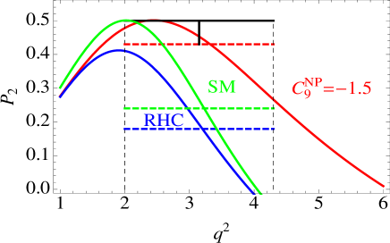
From this observation we conclude that any CP-conserving new-physics contribution added to the Wilson-coefficients 𝑪𝟕,𝟗,𝟏𝟎subscript𝑪7910C_{7,9,10} will shift the position 𝒒𝟏𝟐superscriptsubscript𝒒12q_{1}^{2} of the maximum of 𝑷𝟐subscript𝑷2P_{2}, while maintaining its height at 𝑷𝟐𝐦𝐚𝐱𝟏/(𝟐𝜷)similar-tosuperscriptsubscript𝑷2𝐦𝐚𝐱12𝜷P_{2}^{\rm max}\sim 1/(2\beta). Compared to the SM-prediction 𝒒𝟏𝟐𝟐𝐆𝐞𝐕𝟐superscriptsubscript𝒒122superscript𝐆𝐞𝐕2q_{1}^{2}\approx 2\,{\rm GeV}^{2}, the experimental result 𝑷𝟐[𝟐,4.3]=0.500.07+0.00subscriptdelimited-⟨⟩subscript𝑷224.3subscriptsuperscript0.500.000.07\langle P_{2}\rangle_{[2,4.3]}=0.50^{+0.00}_{-0.07} prefers a larger value for 𝒒𝟏𝟐superscriptsubscript𝒒12q_{1}^{2}, more to the center of the bin [𝟐,4.3]24.3[2,4.3] GeV2. This pull to larger 𝒒𝟐superscript𝒒2q^{2}-values for the position of the maximum of 𝑷𝟐subscript𝑷2P_{2} is consistent with the pull to larger 𝒒𝟐superscript𝒒2q^{2}-values of its zero mentioned in the introduction. From Eq. (29) we see that a larger 𝒒𝟏𝟐superscriptsubscript𝒒12q_{1}^{2} can be obtained by a negative NP contribution to 𝑪𝟗subscript𝑪9C_{9}, as required by the 𝑷𝟓superscriptsubscript𝑷5bold-′P_{5}^{\prime} anomaly, and/or by a positive contribution to 𝑪𝟏𝟎subscript𝑪10C_{10}. Notice further that, while it was claimed in Ref. zwicky that charm-loop effects might affect the position of the zero of 𝑷𝟐subscript𝑷2P_{2}, their impact on the position of the maximum is basically negligible for all scenarios studied in Ref. zwicky . In general, the maximum of 𝑷𝟐subscript𝑷2P_{2} probes the Wilson coefficient 𝑪𝟗𝐞𝐟𝐟superscriptsubscript𝑪9𝐞𝐟𝐟C_{9}^{\rm eff} in a different region in 𝒒𝟐superscript𝒒2q^{2} than the 𝑷𝟓superscriptsubscript𝑷5bold-′P_{5}^{\prime} anomaly or the zero of 𝑷𝟐subscript𝑷2P_{2}. While a potential NP contribution to 𝑪𝟗𝐞𝐟𝐟superscriptsubscript𝑪9𝐞𝐟𝐟C_{9}^{\rm eff} is 𝒒𝟐superscript𝒒2q^{2}-independent and thus induces exactly related effects in the three observables, a charm-loop contribution enters 𝑪𝟗𝐞𝐟𝐟superscriptsubscript𝑪9𝐞𝐟𝐟C_{9}^{\rm eff} as a non-trivial function of 𝒒𝟐superscript𝒒2q^{2} which is expected to decrease with increasing distance to the 𝒄𝒄¯𝒄bold-¯𝒄c\bar{c} resonance region. A measurement of the maximum of 𝑷𝟐subscript𝑷2P_{2} can thus help to discriminate between NP at high energies and non-perturbative charm effects, and the upcoming data with smaller-sized bins will help to determine it more precisely.

In contrast to 𝑪𝟕,𝟗,𝟏𝟎subscript𝑪7910C_{7,9,10}, a new right-handed contribution to one of the Wilson coefficients 𝑪𝟕,𝟗,𝟏𝟎superscriptsubscript𝑪7910bold-′C_{7,9,10}^{\prime} will not only shift the position 𝒒𝟏𝟐superscriptsubscript𝒒12q_{1}^{2} of the maximum of 𝑷𝟐subscript𝑷2P_{2} but will also lower its value 𝑷𝟐𝐦𝐚𝐱superscriptsubscript𝑷2𝐦𝐚𝐱P_{2}^{\rm max}, pushing it below 𝟏/(𝟐𝜷)12𝜷1/(2\beta) Becirevic:2011bp . At leading order, this can be seen from the fact that in the presence of right-handed currents the identity 𝑨𝑹=𝑨𝑹superscriptsubscript𝑨perpendicular-to𝑹superscriptsubscript𝑨bold-∥𝑹A_{\perp}^{R}=-A_{\|}^{R} does not hold anymore for all 𝒒𝟐superscript𝒒2q^{2} so that the two conditions 𝑨𝑳(𝒒𝟏𝟐)=𝑨𝑳(𝒒𝟏𝟐)superscriptsubscript𝑨perpendicular-to𝑳superscriptsubscript𝒒12superscriptsubscript𝑨bold-∥𝑳superscriptsubscript𝒒12A_{\perp}^{L}(q_{1}^{2})=A_{\|}^{L}(q_{1}^{2}) and 𝑨𝑹(𝒒𝟏𝟐)=𝑨𝑹(𝒒𝟏𝟐)superscriptsubscript𝑨perpendicular-to𝑹superscriptsubscript𝒒12superscriptsubscript𝑨bold-∥𝑹superscriptsubscript𝒒12A_{\perp}^{R}(q_{1}^{2})=-A_{\|}^{R}(q_{1}^{2}) required for 𝑷𝟐(𝒒𝟏𝟐)=𝟏/(𝟐𝜷)subscript𝑷2superscriptsubscript𝒒1212𝜷P_{2}(q_{1}^{2})=1/(2\beta) cannot be fulfilled at the same point 𝒒𝟏𝟐superscriptsubscript𝒒12q_{1}^{2}. In general, right-handed currents will cause |𝒏(𝒒𝟏𝟐)||𝒏(𝒒𝟏𝟐)|subscript𝒏perpendicular-tosuperscriptsubscript𝒒12subscript𝒏bold-∥superscriptsubscript𝒒12|n_{\perp}(q_{1}^{2})|\not=|n_{\|}(q_{1}^{2})| and thus induce a substantial non-vanishing 𝑷𝟏(𝒒𝟏𝟐)subscript𝑷1superscriptsubscript𝒒12P_{1}(q_{1}^{2}), preventing 𝑷𝟐(𝒒𝟐𝟐)subscript𝑷2superscriptsubscript𝒒22P_{2}(q_{2}^{2}) from reaching its absolute maximum 𝟏/(𝟐𝜷)12𝜷1/(2\beta).

Refer to caption
Refer to caption
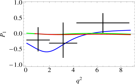
Figure 1: Left: Comparison of the 𝑷𝟐subscript𝑷2P_{2}-curves (central values) in the SM (green) and in two scenarios of New Physics. The scenario NP (red) corresponds to 𝑪𝟗𝐍𝐏=1.5superscriptsubscript𝑪9𝐍𝐏1.5C_{9}^{\rm NP}=-1.5, the scenario RHC (blue) corresponds to 𝑪𝟗=𝟏superscriptsubscript𝑪9bold-′1C_{9}^{\prime}=1, 𝑪𝟏𝟎=0.4superscriptsubscript𝑪10bold-′0.4C_{10}^{\prime}=0.4, 𝑪𝟕=0.06superscriptsubscript𝑪7bold-′0.06C_{7}^{\prime}=0.06. Dashed lines represent the central value for the integrated bin [𝟐,4.3]24.3[2,4.3] GeV2 of the respective curve, while the black cross indicates the measured value in this bin. Right: The analogous curves for 𝑷𝟏subscript𝑷1P_{1} with the black crosses representing the measured values in the respective bins.

In order to illustrate the discriminating power of the bin [𝟐,4.3]24.3[2,4.3] GeV2 of 𝑷𝟐subscript𝑷2P_{2}, we show on the left-hand side of Fig. 1 the curve of 𝑷𝟐subscript𝑷2P_{2} (central value) in the neighbourhood of its maximum together with the integrated result for three different scenarios: the SM, a new physics scenario NP with 𝑪𝟗𝐍𝐏=1.5superscriptsubscript𝑪9𝐍𝐏1.5C_{9}^{\rm NP}=-1.5, and a new physics scenario RHC with the right-handed currents 𝑪𝟕=0.06superscriptsubscript𝑪7bold-′0.06C_{7}^{\prime}=0.06, 𝑪𝟗=𝟏superscriptsubscript𝑪9bold-′1C_{9}^{\prime}=1, 𝑪𝟏𝟎=0.4superscriptsubscript𝑪10bold-′0.4C_{10}^{\prime}=0.4. In the scenario NP, the maximum of 𝑷𝟐subscript𝑷2P_{2} is not lowered but its position is shifted to a higher 𝒒𝟐superscript𝒒2q^{2}-value leading to a better agreement of the integrated result with the measured value. In the scenario RHC, on the other hand, the height of the maximum is lowered resulting in a stronger deviation of the integrated result from the measured value compared to the SM case. The scenario RHC has been chosen in such a way that the central values for all low-𝒒𝟐superscript𝒒2q^{2} bins of 𝑷𝟏subscript𝑷1P_{1} fall within the experimental 1𝝈𝝈\sigma regions, as demonstrated in the plot on the right-hand side of Fig. 1. It thus constitutes an illustrative example of a setup with new right-handed currents to which the maximum of 𝑷𝟐subscript𝑷2P_{2} exhibits a stronger sensitivity than the observable 𝑷𝟏subscript𝑷1P_{1}.

IV.2 Relation between 𝑷𝟒superscriptsubscript𝑷4bold-′P_{4}^{\prime} and 𝑷𝟓superscriptsubscript𝑷5bold-′P_{5}^{\prime} at the position of maximum and at the zero of 𝑷𝟐subscript𝑷2P_{2}

Eq. (21) is quadratic in the parameters 𝑷𝟒superscriptsubscript𝑷4bold-′P_{4}^{\prime},𝑷𝟓superscriptsubscript𝑷5bold-′P_{5}^{\prime},𝑷𝟔superscriptsubscript𝑷6bold-′P_{6}^{\prime},𝑷𝟖superscriptsubscript𝑷8bold-′P_{8}^{\prime}. The requirement of real solutions for these observables constrains the allowed ranges of possible values. For example, demanding a real solution for 𝑷𝟒superscriptsubscript𝑷4bold-′P_{4}^{\prime} from Eq. (21) implies

𝟎𝚫(𝑷𝟒)=𝟒𝒙(𝑷𝟓)𝟐𝟒𝒙(𝑷𝟖)𝟐𝟒[(𝒌𝑻+𝑷𝟏)𝑷𝟔𝟐𝑷𝟐𝑷𝟖𝟐𝑷𝟑𝑷𝟓]𝟐+𝟒𝒙𝒌𝑳(𝒌𝑻𝑷𝟏),0𝚫superscriptsubscript𝑷4bold-′4𝒙superscriptsuperscriptsubscript𝑷5bold-′24𝒙superscriptsuperscriptsubscript𝑷8bold-′24superscriptdelimited-[]subscript𝒌𝑻subscript𝑷1superscriptsubscript𝑷6bold-′2subscript𝑷2superscriptsubscript𝑷8bold-′2subscript𝑷3superscriptsubscript𝑷5bold-′24𝒙subscript𝒌𝑳subscript𝒌𝑻subscript𝑷10\leq\Delta(P_{4}^{\prime})=-4x(P_{5}^{\prime})^{2}-4x(P_{8}^{\prime})^{2}-4\left[(k_{T}+P_{1})P_{6}^{\prime}-2P_{2}P_{8}^{\prime}-2P_{3}P_{5}^{\prime}\right]^{2}+4xk_{L}(k_{T}-P_{1}), (30)

with 𝒙𝒙x defined in eq. (27) and fulfilling 𝒙𝟎𝒙0x\geq 0. Hence, the first three terms in eq. (30) are negative definite and each of them has thus to be smaller in absolute value than the positive fourth term. From this observation we can directly read off constraints on |𝑷𝟓|superscriptsubscript𝑷5bold-′|P_{5}^{\prime}| and |𝑷𝟖|superscriptsubscript𝑷8bold-′|P_{8}^{\prime}|, while constraints on |𝑷𝟒|superscriptsubscript𝑷4bold-′|P_{4}^{\prime}| and |𝑷𝟔|superscriptsubscript𝑷6bold-′|P_{6}^{\prime}| can for example be obtained by considering 𝚫(𝑷𝟓)𝚫superscriptsubscript𝑷5bold-′\Delta(P_{5}^{\prime}). The total set of constraints is given by

|𝑷𝟒|𝒌𝑳(𝒌𝑻𝑷𝟏),|𝑷𝟓|𝟏𝜷𝒌𝑳(𝒌𝑻+𝑷𝟏),|𝑷𝟔|𝟏𝜷𝒌𝑳(𝒌𝑻𝑷𝟏),|𝑷𝟖|𝒌𝑳(𝒌𝑻+𝑷𝟏).formulae-sequencesuperscriptsubscript𝑷4bold-′subscript𝒌𝑳subscript𝒌𝑻subscript𝑷1formulae-sequencesuperscriptsubscript𝑷5bold-′1𝜷subscript𝒌𝑳subscript𝒌𝑻subscript𝑷1formulae-sequencesuperscriptsubscript𝑷6bold-′1𝜷subscript𝒌𝑳subscript𝒌𝑻subscript𝑷1superscriptsubscript𝑷8bold-′subscript𝒌𝑳subscript𝒌𝑻subscript𝑷1|P_{4}^{\prime}|\leq\sqrt{k_{L}(k_{T}-P_{1})},\hskip 19.91684pt|P_{5}^{\prime}|\leq\frac{1}{\beta}\sqrt{k_{L}(k_{T}+P_{1})},\hskip 19.91684pt|P_{6}^{\prime}|\leq\frac{1}{\beta}\sqrt{k_{L}(k_{T}-P_{1})},\hskip 19.91684pt|P_{8}^{\prime}|\leq\sqrt{k_{L}(k_{T}+P_{1})}. (31)

As before, these bounds (with the reinstalled 𝜷𝜷\beta-dependence for 𝑷𝟓superscriptsubscript𝑷5bold-′P_{5}^{\prime} and 𝑷𝟔superscriptsubscript𝑷6bold-′P_{6}^{\prime}) are valid up to quadratic terms in CP-violating coefficients, while exact versions can be obtained via the replacement rules (25) and (26). The constraints are obtained for 𝒙>𝟎𝒙0x>0 and thus are valid for any 𝒒𝟐superscript𝒒2q^{2} except for the single point where 𝒙𝒙x reaches its minimum value 𝒙=𝟎𝒙0x=0. Continuity of the 𝑷𝒊superscriptsubscript𝑷𝒊bold-′P_{i}^{\prime} then implies the bounds to be valid also for 𝒙=𝟎𝒙0x=0.

In the limit 𝒙𝟎bold-→𝒙0x\to 0 the third term in eq. (30) has to vanish in order to render 𝑷𝟒superscriptsubscript𝑷4bold-′P_{4}^{\prime} real. Proceeding in the same way for the other 𝚫(𝑷𝟓,𝟔,𝟖)𝚫superscriptsubscript𝑷568bold-′\Delta(P_{5,6,8}^{\prime}) we obtain four relations at 𝒒𝟐=𝒒𝟏𝟐superscript𝒒2superscriptsubscript𝒒12q^{2}=q_{1}^{2} with 𝒙(𝒒𝟏𝟐)=𝟎𝒙superscriptsubscript𝒒120x(q_{1}^{2})=0:

[(𝒌𝑻+𝑷𝟏)𝑷𝟔𝟐𝑷𝟐𝑷𝟖𝟐𝑷𝟑𝑷𝟓]𝒒𝟏𝟐subscriptdelimited-[]subscript𝒌𝑻subscript𝑷1superscriptsubscript𝑷6bold-′2subscript𝑷2superscriptsubscript𝑷8bold-′2subscript𝑷3superscriptsubscript𝑷5bold-′superscriptsubscript𝒒12\displaystyle\left[(k_{T}+P_{1})P_{6}^{\prime}-2P_{2}P_{8}^{\prime}-2P_{3}P_{5}^{\prime}\right]_{q_{1}^{2}} =\displaystyle= 𝟎,0\displaystyle 0,
[(𝒌𝑻𝑷𝟏)𝑷𝟖𝟐𝑷𝟐𝑷𝟔+𝟐𝑷𝟑𝑷𝟒]𝒒𝟏𝟐subscriptdelimited-[]subscript𝒌𝑻subscript𝑷1superscriptsubscript𝑷8bold-′2subscript𝑷2superscriptsubscript𝑷6bold-′2subscript𝑷3superscriptsubscript𝑷4bold-′superscriptsubscript𝒒12\displaystyle\left[(k_{T}-P_{1})P_{8}^{\prime}-2P_{2}P_{6}^{\prime}+2P_{3}P_{4}^{\prime}\right]_{q_{1}^{2}} =\displaystyle= 𝟎,0\displaystyle 0,
[(𝒌𝑻+𝑷𝟏)𝑷𝟒𝟐𝑷𝟐𝑷𝟓+𝟐𝑷𝟑𝑷𝟖]𝒒𝟏𝟐subscriptdelimited-[]subscript𝒌𝑻subscript𝑷1superscriptsubscript𝑷4bold-′2subscript𝑷2superscriptsubscript𝑷5bold-′2subscript𝑷3superscriptsubscript𝑷8bold-′superscriptsubscript𝒒12\displaystyle\left[(k_{T}+P_{1})P_{4}^{\prime}-2P_{2}P_{5}^{\prime}+2P_{3}P_{8}^{\prime}\right]_{q_{1}^{2}} =\displaystyle= 𝟎,0\displaystyle 0,
[(𝒌𝑻𝑷𝟏)𝑷𝟓𝟐𝑷𝟐𝑷𝟒𝟐𝑷𝟑𝑷𝟔]𝒒𝟏𝟐subscriptdelimited-[]subscript𝒌𝑻subscript𝑷1superscriptsubscript𝑷5bold-′2subscript𝑷2superscriptsubscript𝑷4bold-′2subscript𝑷3superscriptsubscript𝑷6bold-′superscriptsubscript𝒒12\displaystyle\left[(k_{T}-P_{1})P_{5}^{\prime}-2P_{2}P_{4}^{\prime}-2P_{3}P_{6}^{\prime}\right]_{q_{1}^{2}} =\displaystyle= 𝟎.0\displaystyle 0. (32)

Neglecting 𝑷𝟑𝑷𝟔,𝟖𝑷𝟐𝑷𝟒,𝟓much-less-thansubscript𝑷3superscriptsubscript𝑷68bold-′subscript𝑷2superscriptsubscript𝑷45bold-′P_{3}P_{6,8}^{\prime}\ll P_{2}P_{4,5}^{\prime} and including the 𝜷𝜷\beta-factor for 𝑷𝟓superscriptsubscript𝑷5bold-′P_{5}^{\prime}, the last two equations reduce to

𝑷𝟒(𝒒𝟏𝟐)=[𝜷𝑷𝟓𝒌𝑻𝑷𝟏𝒌𝑻+𝑷𝟏]𝒒𝟏𝟐.superscriptsubscript𝑷4bold-′superscriptsubscript𝒒12subscriptdelimited-[]𝜷superscriptsubscript𝑷5bold-′subscript𝒌𝑻subscript𝑷1subscript𝒌𝑻subscript𝑷1superscriptsubscript𝒒12P_{4}^{\prime}(q_{1}^{2})=\left[\beta P_{5}^{\prime}\sqrt{\frac{k_{T}-P_{1}}{k_{T}+P_{1}}}\right]_{q_{1}^{2}}. (33)

This relation is valid at the zero 𝒒𝟏𝟐superscriptsubscript𝒒12q_{1}^{2} of 𝒙𝒙x where 𝑷𝟐=𝒌𝑻𝟐𝑷𝟏𝟐/𝟐𝜷subscript𝑷2superscriptsubscript𝒌𝑻2superscriptsubscript𝑷122𝜷P_{2}=\sqrt{k_{T}^{2}-P_{1}^{2}}/2\beta. For 𝑷𝟏𝟏much-less-thansubscript𝑷11P_{1}\ll 1, which is an excellent approximation in the absence of new right-handed currents, 𝒒𝟏𝟐superscriptsubscript𝒒12q_{1}^{2} coincides with the position of the maximum 𝑷𝟐𝐦𝐚𝐱𝒌𝑻/(𝟐𝜷)superscriptsubscript𝑷2𝐦𝐚𝐱subscript𝒌𝑻2𝜷P_{2}^{\rm max}\approx k_{T}/(2\beta) of 𝑷𝟐subscript𝑷2P_{2}, and Eq. (33) becomes

𝑷𝟒(𝒒𝟏𝟐)=𝜷(𝒒𝟏𝟐)𝑷𝟓(𝒒𝟏𝟐).superscriptsubscript𝑷4bold-′superscriptsubscript𝒒12𝜷superscriptsubscript𝒒12superscriptsubscript𝑷5bold-′superscriptsubscript𝒒12P_{4}^{\prime}(q_{1}^{2})\,=\,\beta(q_{1}^{2})P_{5}^{\prime}(q_{1}^{2}). (34)

While Eq. (33) is model-independent, Eq. (34) only applies if there are no new right-handed currents. Its experimental validation therefore provides a test on the size of right-handed currents.

An analogous relation between 𝑷𝟒superscriptsubscript𝑷4bold-′P_{4}^{\prime} and 𝑷𝟓superscriptsubscript𝑷5bold-′P_{5}^{\prime} at the position 𝒒𝟐=𝒒𝟎𝟐superscript𝒒2superscriptsubscript𝒒02q^{2}=q_{0}^{2} of the zero of 𝑷𝟐subscript𝑷2P_{2} was derived and discussed in Ref. nicola . We reproduce it here for completeness. Dropping quadratic terms in 𝑷𝟑subscript𝑷3P_{3}, 𝑷𝟔,𝟖subscript𝑷68P_{6,8} and in the 𝑷𝒊𝐂𝐏superscriptsubscript𝑷𝒊𝐂𝐏P_{i}^{\rm CP} it reads

[𝑷𝟒𝟐+𝜷𝟐𝑷𝟓𝟐]𝒒𝟎𝟐=𝟏𝜼(𝒒𝟎𝟐),subscriptdelimited-[]superscriptsubscript𝑷42superscript𝜷2superscriptsubscript𝑷52superscriptsubscript𝒒021𝜼superscriptsubscript𝒒02[{P_{4}}^{\prime 2}+\beta^{2}{P_{5}^{\prime 2}}]_{q_{0}^{2}}=1-\eta(q_{0}^{2}), (35)

where 𝜼(𝒒𝟎𝟐)=[𝑷𝟏𝟐+𝑷𝟏(𝑷𝟒𝟐𝜷𝟐𝑷𝟓𝟐)]𝒒𝟎𝟐𝜼superscriptsubscript𝒒02subscriptdelimited-[]superscriptsubscript𝑷12subscript𝑷1superscriptsubscript𝑷42superscript𝜷2superscriptsubscript𝑷52superscriptsubscript𝒒02\eta(q_{0}^{2})=[{P_{1}}^{2}+{P_{1}}({P_{4}}^{\prime 2}-\beta^{2}{P_{5}}^{\prime 2})]_{q_{0}^{2}} is completely negligible (of order 𝜼(𝒒𝟎𝟐)𝟏𝟎𝟑similar-to𝜼superscriptsubscript𝒒02superscript103\eta(q_{0}^{2})\sim 10^{-3}) in the absence of new right-handed currents. Let us assume that, as data seem to suggest, the zero 𝒒𝟎𝟐superscriptsubscript𝒒02q_{0}^{2} of 𝑷𝟐subscript𝑷2P_{2} would be larger than predicted by the SM. In this case, Eq. (35) forces the absolute value of 𝑷𝟓(𝒒𝟎𝟐)superscriptsubscript𝑷5bold-′superscriptsubscript𝒒02P_{5}^{\prime}(q_{0}^{2}) to be smaller than in the SM, in agreement with the anomaly.

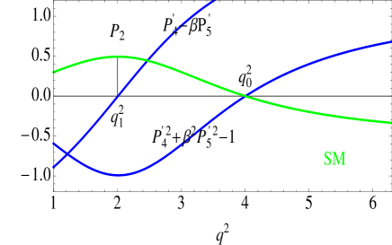
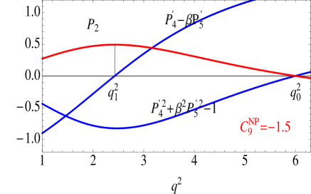
In Fig. 2 we show central values of the theory predictions for the two functions 𝑷𝟒𝜷𝑷𝟓superscriptsubscript𝑷4bold-′𝜷superscriptsubscript𝑷5bold-′P_{4}^{\prime}-\beta P_{5}^{\prime} and (𝑷𝟒)𝟐+𝜷𝟐(𝑷𝟓)𝟐𝟏superscriptsuperscriptsubscript𝑷4bold-′2superscript𝜷2superscriptsuperscriptsubscript𝑷5bold-′21(P_{4}^{\prime})^{2}+\beta^{2}(P_{5}^{\prime})^{2}-1 for the SM and the new-physics scenario NP with 𝑪𝟗𝐍𝐏=1.5superscriptsubscript𝑪9𝐍𝐏1.5C_{9}^{\rm NP}=-1.5. The zeros of the corresponding curves at 𝒒𝟐=𝒒𝟏𝟐superscript𝒒2superscriptsubscript𝒒12q^{2}=q_{1}^{2} and 𝒒𝟐=𝒒𝟎𝟐superscript𝒒2superscriptsubscript𝒒02q^{2}=q_{0}^{2}, respectively, demonstrate that the relations (34) and (35) are indeed fulfilled to excellent precision.
Refer to caption
Refer to caption
Figure 2: Illustration of the relations (34) and (35) between the observables 𝑷𝟒superscriptsubscript𝑷4bold-′P_{4}^{\prime} and 𝑷𝟓superscriptsubscript𝑷5bold-′P_{5}^{\prime} (central values) at the position of the maximum and the zero of 𝑷𝟐subscript𝑷2P_{2}. Left: SM. Right: scenario NP with 𝑪𝟗𝐍𝐏=1.5superscriptsubscript𝑪9𝐍𝐏1.5C_{9}^{\rm NP}=-1.5.

IV.3 Constraints on the 𝑨𝑺(𝒊)superscriptsubscript𝑨𝑺𝒊A_{S}^{(i)} and relations at the position of the maximum and the zero of 𝑷𝟐subscript𝑷2P_{2}

Eq. (22) is quadratic in the parameters 𝑨𝑺𝟒superscriptsubscript𝑨𝑺4A_{S}^{4},𝑨𝑺𝟓superscriptsubscript𝑨𝑺5A_{S}^{5},𝑨𝑺𝟕superscriptsubscript𝑨𝑺7A_{S}^{7},𝑨𝑺𝟖superscriptsubscript𝑨𝑺8A_{S}^{8}. The requirement of real solutions for these observables constrains the allowed ranges of possible values. Following the procedure described in Sec. IV.2 for the 𝑷𝒊superscriptsubscript𝑷𝒊bold-′P_{i}^{\prime}, we find in a completely analogous manner the bounds

|𝑨𝑺𝟒|𝟏𝟐𝟑𝒌𝑺𝑭𝑻𝑭𝑺(𝟏𝑭𝑺)(𝒌𝑻𝑷𝟏),|𝑨𝑺𝟓|𝟑𝒌𝑺𝑭𝑻𝑭𝑺(𝟏𝑭𝑺)(𝒌𝑻+𝑷𝟏),formulae-sequencesuperscriptsubscript𝑨𝑺4123subscript𝒌𝑺subscript𝑭𝑻subscript𝑭𝑺1subscript𝑭𝑺subscript𝒌𝑻subscript𝑷1superscriptsubscript𝑨𝑺53subscript𝒌𝑺subscript𝑭𝑻subscript𝑭𝑺1subscript𝑭𝑺subscript𝒌𝑻subscript𝑷1\displaystyle|A_{S}^{4}|\leq\frac{1}{2}\sqrt{3k_{S}F_{T}F_{S}(1-F_{S})(k_{T}-P_{1})},\hskip 56.9055pt|A_{S}^{5}|\leq\sqrt{3k_{S}F_{T}F_{S}(1-F_{S})(k_{T}+P_{1})},
|𝑨𝑺𝟕|𝟑𝒌𝑺𝑭𝑻𝑭𝑺(𝟏𝑭𝑺)(𝒌𝑻𝑷𝟏),|𝑨𝑺𝟖|𝟏𝟐𝟑𝒌𝑺𝑭𝑻𝑭𝑺(𝟏𝑭𝑺)(𝒌𝑻+𝑷𝟏).formulae-sequencesuperscriptsubscript𝑨𝑺73subscript𝒌𝑺subscript𝑭𝑻subscript𝑭𝑺1subscript𝑭𝑺subscript𝒌𝑻subscript𝑷1superscriptsubscript𝑨𝑺8123subscript𝒌𝑺subscript𝑭𝑻subscript𝑭𝑺1subscript𝑭𝑺subscript𝒌𝑻subscript𝑷1\displaystyle|A_{S}^{7}|\leq\sqrt{3k_{S}F_{T}F_{S}(1-F_{S})(k_{T}-P_{1})},\hskip 62.59596pt|A_{S}^{8}|\leq\frac{1}{2}\sqrt{3k_{S}F_{T}F_{S}(1-F_{S})(k_{T}+P_{1})}. (36)

Combining further the Eqs. (21)-(23), one obtains a similar bound on 𝑨𝑺subscript𝑨𝑺A_{S} (see Appendix B for a detailed derivation):

|𝑨𝑺|𝟐𝟑𝒌𝑳𝒌𝑺𝑭𝑺(𝟏𝑭𝑺)(𝟏𝑭𝑻)subscript𝑨𝑺23subscript𝒌𝑳subscript𝒌𝑺subscript𝑭𝑺1subscript𝑭𝑺1subscript𝑭𝑻|A_{S}|\leq 2\sqrt{3k_{L}k_{S}F_{S}(1-F_{S})(1-F_{T})} (37)

The constraints (IV.3) and (37) are identical to the ones given in eq. (51) of Ref. optimized up to the Breit-Wigner factor 𝑭=𝒁/𝑿𝒀𝑭𝒁𝑿𝒀F=Z/\sqrt{XY} present in the latter. The results of Ref. optimized were derived using a different method based on the Cauchy-Schwartz inequality. The factor 𝑭𝑭F is a consequence of the implicit assumption of a narrow S-wave resonance made in Ref. optimized , and it has to be replaced by its upper limit 𝑭𝐦𝐚𝐱=𝟏subscript𝑭𝐦𝐚𝐱1F_{\rm max}=1 in the general case. This subtlety has little impact on the numerical results given in Ref. optimized as the phenomenological analysis there was performed taking 𝑭=0.9𝟏𝑭0.91F=0.9\approx 1. We further note that once again the stated results in Eqs. (IV.3) and (37) are valid up to quadratic terms in CP-violating coefficients, with exact versions being obtained via the replacements (25) and (26).
Refer to caption
Refer to caption
Refer to caption
Refer to caption
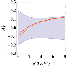
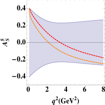
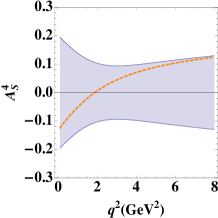
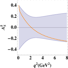
Figure 3: Illustration of the constraints on 𝑨𝑺𝟒,𝟓superscriptsubscript𝑨𝑺45A_{S}^{4,5} obtained from relation (22) in the SM (left two plots) and in the presence of 𝑪𝟗𝐍𝐏=1.5superscriptsubscript𝑪9𝐍𝐏1.5C_{9}^{\rm NP}=-1.5 (right two plots). Blue bands correspond to the uncorrelated bounds from eq. (IV.3). Dashed lines illustrate the correlation between 𝑨𝑺𝟒superscriptsubscript𝑨𝑺4A_{S}^{4} and 𝑨𝑺𝟓superscriptsubscript𝑨𝑺5A_{S}^{5} obtained from relation (22) for the scenario described in the text (orange for the SM, red for 𝑪𝟗𝐍𝐏=1.5superscriptsubscript𝑪9𝐍𝐏1.5C_{9}^{\rm NP}=-1.5).

Proceeding in an analogous way as in the P-wave case in Sec. IV.2, we find also for the S-wave parameters relations at the position 𝒒𝟐=𝒒𝟏𝟐superscript𝒒2superscriptsubscript𝒒12q^{2}=q_{1}^{2} of the zero of the observable 𝒙𝒙x. The corresponding equations read

[(𝒌𝑻+𝑷𝟏)𝑨𝑺𝟕𝟒𝑷𝟐𝑨𝑺𝟖+𝟐𝑷𝟑𝑨𝑺𝟓]𝒒𝟏𝟐subscriptdelimited-[]subscript𝒌𝑻subscript𝑷1superscriptsubscript𝑨𝑺74subscript𝑷2superscriptsubscript𝑨𝑺82subscript𝑷3superscriptsubscript𝑨𝑺5superscriptsubscript𝒒12\displaystyle\left[(k_{T}+P_{1})A_{S}^{7}-4P_{2}A_{S}^{8}+2P_{3}A_{S}^{5}\right]_{q_{1}^{2}} =\displaystyle= 𝟎,0\displaystyle 0,
[(𝒌𝑻𝑷𝟏)𝑨𝑺𝟖𝑷𝟐𝑨𝑺𝟕𝟐𝑷𝟑𝑨𝑺𝟒]𝒒𝟏𝟐subscriptdelimited-[]subscript𝒌𝑻subscript𝑷1superscriptsubscript𝑨𝑺8subscript𝑷2superscriptsubscript𝑨𝑺72subscript𝑷3superscriptsubscript𝑨𝑺4superscriptsubscript𝒒12\displaystyle\left[(k_{T}-P_{1})A_{S}^{8}-P_{2}A_{S}^{7}-2P_{3}A_{S}^{4}\right]_{q_{1}^{2}} =\displaystyle= 𝟎,0\displaystyle 0,
[(𝒌𝑻+𝑷𝟏)𝑨𝑺𝟒𝑷𝟐𝑨𝑺𝟓𝟐𝑷𝟑𝑨𝑺𝟖]𝒒𝟏𝟐subscriptdelimited-[]subscript𝒌𝑻subscript𝑷1superscriptsubscript𝑨𝑺4subscript𝑷2superscriptsubscript𝑨𝑺52subscript𝑷3superscriptsubscript𝑨𝑺8superscriptsubscript𝒒12\displaystyle\left[(k_{T}+P_{1})A_{S}^{4}-P_{2}A_{S}^{5}-2P_{3}A_{S}^{8}\right]_{q_{1}^{2}} =\displaystyle= 𝟎,0\displaystyle 0,
[(𝒌𝑻𝑷𝟏)𝑨𝑺𝟓𝟒𝑷𝟐𝑨𝑺𝟒+𝟐𝑷𝟑𝑨𝑺𝟕]𝒒𝟏𝟐subscriptdelimited-[]subscript𝒌𝑻subscript𝑷1superscriptsubscript𝑨𝑺54subscript𝑷2superscriptsubscript𝑨𝑺42subscript𝑷3superscriptsubscript𝑨𝑺7superscriptsubscript𝒒12\displaystyle\left[(k_{T}-P_{1})A_{S}^{5}-4P_{2}A_{S}^{4}+2P_{3}A_{S}^{7}\right]_{q_{1}^{2}} =\displaystyle= 𝟎,0\displaystyle 0, (38)

and simplify to

𝟐𝑨𝑺𝟒(𝒒𝟏𝟐)=[𝑨𝑺𝟓𝒌𝑻𝑷𝟏𝒌𝑻+𝑷𝟏]𝒒𝟏𝟐and𝑨𝑺𝟕(𝒒𝟏𝟐)=[𝟐𝑨𝑺𝟖𝒌𝑻𝑷𝟏𝒌𝑻+𝑷𝟏]𝒒𝟏𝟐formulae-sequence2superscriptsubscript𝑨𝑺4superscriptsubscript𝒒12subscriptdelimited-[]superscriptsubscript𝑨𝑺5subscript𝒌𝑻subscript𝑷1subscript𝒌𝑻subscript𝑷1superscriptsubscript𝒒12andsuperscriptsubscript𝑨𝑺7superscriptsubscript𝒒12subscriptdelimited-[]2superscriptsubscript𝑨𝑺8subscript𝒌𝑻subscript𝑷1subscript𝒌𝑻subscript𝑷1superscriptsubscript𝒒122A_{S}^{4}(q_{1}^{2})=\left[A_{S}^{5}\sqrt{\frac{k_{T}-P_{1}}{k_{T}+P_{1}}}\right]_{q_{1}^{2}}\hskip 42.67912pt\text{and}\hskip 42.67912ptA_{S}^{7}(q_{1}^{2})=\left[2A_{S}^{8}\sqrt{\frac{k_{T}-P_{1}}{k_{T}+P_{1}}}\right]_{q_{1}^{2}} (39)

under the assumption of 𝑷𝟑𝑨𝑺𝒊𝑷𝟐𝑨𝑺𝒋much-less-thansubscript𝑷3superscriptsubscript𝑨𝑺𝒊subscript𝑷2superscriptsubscript𝑨𝑺𝒋P_{3}A_{S}^{i}\ll P_{2}A_{S}^{j}. For 𝑷𝟏𝟏much-less-thansubscript𝑷11P_{1}\ll 1, one obtains at the position 𝒒𝟏𝟐superscriptsubscript𝒒12q_{1}^{2} of the maximum of 𝑷𝟐subscript𝑷2P_{2}:

𝟐𝑨𝑺𝟒(𝒒𝟏𝟐)=𝑨𝑺𝟓(𝒒𝟏𝟐)and𝑨𝑺𝟕(𝒒𝟏𝟐)=𝟐𝑨𝑺𝟖(𝒒𝟏𝟐).formulae-sequence2superscriptsubscript𝑨𝑺4superscriptsubscript𝒒12superscriptsubscript𝑨𝑺5superscriptsubscript𝒒12andsuperscriptsubscript𝑨𝑺7superscriptsubscript𝒒122superscriptsubscript𝑨𝑺8superscriptsubscript𝒒122A_{S}^{4}(q_{1}^{2})=A_{S}^{5}(q_{1}^{2})\hskip 42.67912pt\text{and}\hskip 42.67912ptA_{S}^{7}(q_{1}^{2})=2A_{S}^{8}(q_{1}^{2}). (40)

The symmetry relation (22), together with the implicitly contained relations (39),(40) at the zero 𝒒𝟏𝟐superscriptsubscript𝒒12q_{1}^{2} of 𝒙𝒙x, imposes correlations among the 𝑨𝑺𝒊superscriptsubscript𝑨𝑺𝒊A_{S}^{i} implying constraints that go beyond the individual bounds given in Eqs. (IV.3),(37). To illustrate this, we assume that a measurement gives 𝑨𝑺𝟕,𝟖𝑨𝑺𝟒,𝟓much-less-thansuperscriptsubscript𝑨𝑺78superscriptsubscript𝑨𝑺45A_{S}^{7,8}\ll A_{S}^{4,5}. In this case, the symmetry relation (22) implies a direct correlation between 𝑨𝑺𝟒superscriptsubscript𝑨𝑺4A_{S}^{4} and 𝑨𝑺𝟓superscriptsubscript𝑨𝑺5A_{S}^{5}. If for example 𝑨𝑺𝟓superscriptsubscript𝑨𝑺5A_{S}^{5} is measured to be 𝑨𝑺𝟓=𝜶𝑷𝟓superscriptsubscript𝑨𝑺5𝜶superscriptsubscript𝑷5bold-′A_{S}^{5}=\alpha P_{5}^{\prime} where 𝜶=𝟑𝑭𝑻𝑭𝑺(𝟏𝑭𝑺)𝒌𝑺/𝒌𝑳𝜶3subscript𝑭𝑻subscript𝑭𝑺1subscript𝑭𝑺subscript𝒌𝑺subscript𝒌𝑳\alpha=\sqrt{3F_{T}F_{S}(1-F_{S})k_{S}/k_{L}}, 𝑨𝑺𝟒superscriptsubscript𝑨𝑺4A_{S}^{4} is completely fixed to 𝑨𝑺𝟒=𝜶𝟐𝑷𝟒superscriptsubscript𝑨𝑺4𝜶2superscriptsubscript𝑷4bold-′A_{S}^{4}=\frac{\alpha}{2}P_{4}^{\prime}. This scenario is illustrated in Fig. 3 for constant 𝑭𝑺𝟔%similar-to-or-equalssubscript𝑭𝑺percent6F_{S}\simeq 6\%. The orange dashed curves in the plots on the left are obtained for SM values of 𝑷𝟒,𝟓superscriptsubscript𝑷45bold-′P_{4,5}^{\prime}, while the red dashed curves in the plots on the right correspond to the presence of 𝑪𝟗𝐍𝐏=1.5superscriptsubscript𝑪9𝐍𝐏1.5C_{9}^{\rm NP}=-1.5 (in addition the SM curve is shown also in the plots on the right to visualize the shift between the two curves). If one of the curves is measured for 𝑨𝑺𝟓superscriptsubscript𝑨𝑺5A_{S}^{5}, the corresponding curve for 𝑨𝑺𝟒superscriptsubscript𝑨𝑺4A_{S}^{4} is predicted by the symmetry relation, and vice versa. Note that also the blue bands corresponding to the uncorrelated bounds from eq. (IV.3) are slightly different in the SM and in the NP case.

As in the previous section for the P-wave observables, we give also for the S-wave observables simplified versions of the symmetry relations at the zero 𝒒𝟐=𝒒𝟎𝟐superscript𝒒2superscriptsubscript𝒒02q^{2}=q_{0}^{2} of 𝑷𝟐subscript𝑷2P_{2}. Neglecting the small 𝑷𝟑,𝑷𝟔,𝟖subscript𝑷3superscriptsubscript𝑷68bold-′{P}_{3},{P}_{6,8}^{\prime} terms, Eqs. (22) and (23) simplify to

[(𝟒𝑨𝑺4 2+𝑨𝑺7 2)(𝟏+𝑷𝟏)+(𝑨𝑺5 2+𝟒𝑨𝑺8 2)(𝟏𝑷𝟏)]𝒒𝟎𝟐=𝟑[(𝟏𝑭𝑺)𝑭𝑺𝑭𝑻(𝟏𝑷𝟏𝟐)]𝒒𝟎𝟐,subscriptdelimited-[]4superscriptsubscript𝑨𝑺42superscriptsubscript𝑨𝑺721subscript𝑷1superscriptsubscript𝑨𝑺524superscriptsubscript𝑨𝑺821subscript𝑷1superscriptsubscript𝒒023subscriptdelimited-[]1subscript𝑭𝑺subscript𝑭𝑺subscript𝑭𝑻1superscriptsubscript𝑷12superscriptsubscript𝒒02[(4A_{S}^{4\,2}+A_{S}^{7\,2})(1+P_{1})+(A_{S}^{5\,2}+4A_{S}^{8\,2})(1-P_{1})]_{q_{0}^{2}}=3[(1-F_{S})F_{S}F_{T}(1-P_{1}^{2})]_{q_{0}^{2}}, (41)
𝑨𝑺(𝒒𝟎𝟐)=[𝟐𝟏𝑭𝑻(𝟐𝑨𝑺𝟒(𝟏+𝑷𝟏)𝑷𝟒+𝑨𝑺𝟓(𝟏𝑷𝟏)𝑷𝟓)𝑭𝑻(𝟏𝑷𝟏𝟐)]𝒒𝟎𝟐.subscript𝑨𝑺superscriptsubscript𝒒02subscriptdelimited-[]21subscript𝑭𝑻2superscriptsubscript𝑨𝑺41subscript𝑷1superscriptsubscript𝑷4bold-′superscriptsubscript𝑨𝑺51subscript𝑷1superscriptsubscript𝑷5bold-′subscript𝑭𝑻1superscriptsubscript𝑷12superscriptsubscript𝒒02A_{S}(q_{0}^{2})=\left[\frac{2\sqrt{1-F_{T}}(2A_{S}^{4}(1+P_{1})P_{4}^{\prime}+A_{S}^{5}(1-P_{1})P_{5}^{\prime})}{\sqrt{F_{T}}(1-P_{1}^{2})}\right]_{q_{0}^{2}}. (42)

V Conclusions

In this article we have exploited the spin symmetry of the angular distribution of the decay 𝑩𝑲𝝁+𝝁bold-→𝑩superscript𝑲superscript𝝁superscript𝝁B\to K^{*}\mu^{+}\mu^{-}, both in the P-wave as well as in the S-wave sector. We have shown that the symmetry reduces the number of independent S-wave observables from six to four, implying two non-trivial relations among the observables 𝑭𝑺subscript𝑭𝑺F_{S}, 𝑨𝑺subscript𝑨𝑺A_{S}, 𝑨𝑺𝟒superscriptsubscript𝑨𝑺4A_{S}^{4}, 𝑨𝑺𝟓superscriptsubscript𝑨𝑺5A_{S}^{5}, 𝑨𝑺𝟕superscriptsubscript𝑨𝑺7A_{S}^{7} and 𝑨𝑺𝟖superscriptsubscript𝑨𝑺8A_{S}^{8} which we derived explicitly. The relations allowed us to obtain individual bounds on the 𝑨𝑺(𝒊)superscriptsubscript𝑨𝑺𝒊A_{S}^{(i)} which agree with the ones determined in Ref. optimized via the Cauchy-Schwartz inequality. However, the constraining power of the symmetry relations goes beyond these individual bounds as they correlate the S-wave observables among each other. The implementation of these correlations into the experimental data analysis is expected to reduce the background from S-wave pollution. As an example, we have shown how for 𝑨𝑺𝟕,𝟖𝑨𝑺𝟒,𝟓much-less-thansuperscriptsubscript𝑨𝑺78superscriptsubscript𝑨𝑺45A_{S}^{7,8}\ll A_{S}^{4,5} the correlations fix 𝑨𝑺𝟒superscriptsubscript𝑨𝑺4A_{S}^{4} from a measurement of 𝑨𝑺𝟓superscriptsubscript𝑨𝑺5A_{S}^{5} and 𝑭𝑺subscript𝑭𝑺F_{S} (or 𝑨𝑺𝟓superscriptsubscript𝑨𝑺5A_{S}^{5} from a measurement of 𝑨𝑺𝟒superscriptsubscript𝑨𝑺4A_{S}^{4} and 𝑭𝑺subscript𝑭𝑺F_{S}) in the whole range of the of the squared dilepton invariant mass 𝒒𝟐superscript𝒒2q^{2}. We further showed that 𝑨𝑺𝟒/𝑨𝑺𝟓superscriptsubscript𝑨𝑺4superscriptsubscript𝑨𝑺5A_{S}^{4}/A_{S}^{5} and 𝑨𝑺𝟕/𝑨𝑺𝟖superscriptsubscript𝑨𝑺7superscriptsubscript𝑨𝑺8A_{S}^{7}/A_{S}^{8} are completely fixed at a point 𝒒𝟐=𝒒𝟏𝟐superscript𝒒2superscriptsubscript𝒒12q^{2}=q_{1}^{2} where 𝒒𝟏𝟐superscriptsubscript𝒒12q_{1}^{2} coincides with the position of the maximum of the P-wave observable 𝑷𝟐subscript𝑷2P_{2} in the absence of new right-handed currents.

We also pointed out the strong potential of the maximum of 𝑷𝟐subscript𝑷2P_{2} for probing NP beyong the SM, in particular the presence of new right-handed currents, in a region far away from charm resonances. We have shown that a shift of the position of the maximum of 𝑷𝟐subscript𝑷2P_{2} compared to its SM expectation, with the height of the maximum 𝑷𝟐𝐦𝐚𝐱superscriptsubscript𝑷2𝐦𝐚𝐱P_{2}^{\rm max} kept at the SM value 𝟏/(𝟐𝜷)12𝜷1/(2\beta), would be a signal of a NP contribution to the SM-like Wilson coefficients 𝑪𝟕subscript𝑪7C_{7}, 𝑪𝟗subscript𝑪9C_{9}, 𝑪𝟏𝟎subscript𝑪10C_{10}. A maximum value 𝑷𝟐𝐦𝐚𝐱<𝟏/(𝟐𝜷)superscriptsubscript𝑷2𝐦𝐚𝐱12𝜷P_{2}^{\rm max}<1/(2\beta), on the other hand, would detect the presence of new right-handed currents and thus complement information from the (currently not very precisely measured) observable 𝑷𝟏subscript𝑷1P_{1}. We have further proven and illustrated that for 𝑪𝟕=𝑪𝟗=𝑪𝟏𝟎=𝟎superscriptsubscript𝑪7bold-′superscriptsubscript𝑪9bold-′superscriptsubscript𝑪10bold-′0C_{7}^{\prime}=C_{9}^{\prime}=C_{10}^{\prime}=0 the angular observables 𝑷𝟒superscriptsubscript𝑷4bold-′P_{4}^{\prime} and 𝑷𝟓superscriptsubscript𝑷5bold-′P_{5}^{\prime} fulfill 𝑷𝟒=𝜷𝑷𝟓superscriptsubscript𝑷4bold-′𝜷superscriptsubscript𝑷5bold-′P_{4}^{\prime}=\beta P_{5}^{\prime} at the position of the maximum of 𝑷𝟐subscript𝑷2P_{2}, so that any deviation from this relation would equally signal the presence of new right-handed currents.


Acknowledgments. We would like to thank K. A. Petridis and N. Serra for many useful discussions. L.H. has been supported by FPA2011-25948 and the grant 2014 SGR 1450, and in part by the Centro de Excelencia Severo Ochoa SEV-2012-0234. J.M. acknowledges financial support from the Explora project FPA2014-61478-EXP.

Appendix A: Gauge conditions for the amplitudes

All the angular observables studied by the LHCb experiment are invariant under a 𝑼(𝟐)𝑼2U(2) rotation of the vectors 𝒏𝒊subscript𝒏𝒊n_{i} defined in Eq. (6). As a consequence, the amplitudes 𝑨𝒊𝑳,𝑹superscriptsubscript𝑨𝒊𝑳𝑹A_{i}^{L,R} cannot be determined unambigously from experiment. In order to arrive at a one-to-one correspondence between the experimental observables and the theoretical amplitudes, one has to fix a convention which picks for every class of 𝑼(𝟐)𝑼2U(2)-related amplitudes a certain representant (similar to ”fixing the gauge”). One convenient choice that has been proposed and is used by the Imperial group of the LHCb experiment Kostas consists in requiring

𝐑𝐞𝑨𝟎𝑹=𝟎,𝐈𝐦𝑨𝟎𝑹=𝟎,𝐈𝐦𝑨𝟎𝑳=𝟎,𝐈𝐦𝑨𝑹=𝟎.formulae-sequence𝐑𝐞superscriptsubscript𝑨0𝑹0formulae-sequence𝐈𝐦superscriptsubscript𝑨0𝑹0formulae-sequence𝐈𝐦superscriptsubscript𝑨0𝑳0𝐈𝐦superscriptsubscript𝑨perpendicular-to𝑹0{\rm Re}A_{0}^{R}=0,\quad{\rm Im}A_{0}^{R}=0,\quad{\rm Im}A_{0}^{L}=0,\quad{\rm Im}A_{\perp}^{R}=0.

This choice is not unique, several combinations are possible (see Ref. ulrik1 for a different choice). Starting from an arbitrary amplitude, one arrives at the above configuration by means of the 𝑼(𝟐)𝑼2U(2) transformation

𝒏𝒊[𝒆𝒊ϕ𝑳𝟎𝟎𝒆𝒊ϕ𝑹][𝐜𝐨𝐬𝜽𝐬𝐢𝐧𝜽𝐬𝐢𝐧𝜽𝐜𝐨𝐬𝜽][𝐜𝐨𝐬𝐡𝒊𝜽~𝐬𝐢𝐧𝐡𝒊𝜽~𝐬𝐢𝐧𝐡𝒊𝜽~𝐜𝐨𝐬𝐡𝒊𝜽~]𝒏𝒊.bold-→subscript𝒏𝒊delimited-[]superscript𝒆𝒊subscriptbold-italic-ϕ𝑳00superscript𝒆𝒊subscriptbold-italic-ϕ𝑹delimited-[]𝜽𝜽𝜽𝜽delimited-[]𝒊bold-~𝜽𝒊bold-~𝜽𝒊bold-~𝜽𝒊bold-~𝜽subscript𝒏𝒊n_{i}\to\left[\begin{array}[]{ll}e^{i\phi_{L}}&0\\ 0&e^{-i\phi_{R}}\end{array}\right]\left[\begin{array}[]{rr}\cos\theta&-\sin\theta\\ \sin\theta&\cos\theta\end{array}\right]\left[\begin{array}[]{rr}\cosh i\tilde{\theta}&-\sinh i\tilde{\theta}\\ -\sinh i\tilde{\theta}&\cosh i\tilde{\theta}\end{array}\right]n_{i}\,.

with

𝐭𝐚𝐧𝟐𝜽~=𝟐𝐈𝐦𝑨𝟎𝑹𝐑𝐞𝑨𝟎𝑳+(𝑳𝑹)|𝑨𝟎𝑹|𝟐|𝑨𝟎𝑳|𝟐,{\tan 2{\tilde{\theta}}}=2\frac{{\rm Im}A_{0}^{R}{\rm Re}A_{0}^{L}+(L\leftrightarrow R)}{|A_{0}^{R}|^{2}-|A_{0}^{L}|^{2}}\,,
𝐭𝐚𝐧𝜽=𝐑𝐞𝑨𝟎𝑹+𝐈𝐦𝑨𝟎𝑳𝐭𝐚𝐧𝜽~𝐑𝐞𝑨𝟎𝑳+𝐈𝐦𝑨𝟎𝑹𝐭𝐚𝐧𝜽~,𝜽𝐑𝐞superscriptsubscript𝑨0𝑹𝐈𝐦superscriptsubscript𝑨0𝑳𝐭𝐚𝐧bold-~𝜽𝐑𝐞superscriptsubscript𝑨0𝑳𝐈𝐦superscriptsubscript𝑨0𝑹𝐭𝐚𝐧bold-~𝜽{\tan\theta}=\frac{{\rm Re}A_{0}^{R}+{\rm Im}A_{0}^{L}{\rm tan}{\tilde{\theta}}}{-{\rm Re}A_{0}^{L}+{\rm Im}A_{0}^{R}{\rm tan}{\tilde{\theta}}}\,,
𝐭𝐚𝐧ϕ𝑳=𝐈𝐦𝑨𝟎𝑳+𝐈𝐦𝑨𝟎𝑹𝐭𝐚𝐧𝜽(𝐑𝐞𝑨𝟎𝑹𝐑𝐞𝑨𝟎𝑳𝐭𝐚𝐧𝜽)𝐭𝐚𝐧𝜽~𝐑𝐞𝑨𝟎𝑳+𝐑𝐞𝑨𝟎𝑹𝐭𝐚𝐧𝜽+(𝐈𝐦𝑨𝟎𝑹+𝐈𝐦𝑨𝟎𝑳𝐭𝐚𝐧𝜽)𝐭𝐚𝐧𝜽~,subscriptbold-italic-ϕ𝑳𝐈𝐦superscriptsubscript𝑨0𝑳𝐈𝐦superscriptsubscript𝑨0𝑹𝜽𝐑𝐞superscriptsubscript𝑨0𝑹𝐑𝐞superscriptsubscript𝑨0𝑳𝜽bold-~𝜽𝐑𝐞superscriptsubscript𝑨0𝑳𝐑𝐞superscriptsubscript𝑨0𝑹𝜽𝐈𝐦superscriptsubscript𝑨0𝑹𝐈𝐦superscriptsubscript𝑨0𝑳𝜽bold-~𝜽{\tan\phi_{L}}=\frac{{\rm Im}A_{0}^{L}+{\rm Im}A_{0}^{R}\tan\theta-({\rm Re}A_{0}^{R}-{\rm Re}A_{0}^{L}\tan\theta)\tan\tilde{\theta}}{-{\rm Re}A_{0}^{L}+{\rm Re}A_{0}^{R}\tan\theta+({\rm Im}A_{0}^{R}+{\rm Im}A_{0}^{L}\tan\theta)\tan\tilde{\theta}}\,,
𝐭𝐚𝐧ϕ𝑹=𝐈𝐦𝑨𝑹+𝐈𝐦𝑨𝑳𝐭𝐚𝐧𝜽(𝐑𝐞𝑨𝑳𝐑𝐞𝑨𝑹𝐭𝐚𝐧𝜽)𝐭𝐚𝐧𝜽~𝐑𝐞𝑨𝑹+𝐑𝐞𝑨𝑳𝐭𝐚𝐧𝜽+(𝐈𝐦𝑨𝑳+𝐈𝐦𝑨𝑹𝐭𝐚𝐧𝜽)𝐭𝐚𝐧𝜽~.subscriptbold-italic-ϕ𝑹𝐈𝐦superscriptsubscript𝑨perpendicular-to𝑹𝐈𝐦superscriptsubscript𝑨perpendicular-to𝑳𝜽𝐑𝐞superscriptsubscript𝑨perpendicular-to𝑳𝐑𝐞superscriptsubscript𝑨perpendicular-to𝑹𝜽bold-~𝜽𝐑𝐞superscriptsubscript𝑨perpendicular-to𝑹𝐑𝐞superscriptsubscript𝑨perpendicular-to𝑳𝜽𝐈𝐦superscriptsubscript𝑨perpendicular-to𝑳𝐈𝐦superscriptsubscript𝑨perpendicular-to𝑹𝜽bold-~𝜽{\tan\phi_{R}}=\frac{{\rm Im}A_{\perp}^{R}+{\rm Im}A_{\perp}^{L}\tan\theta-({\rm Re}A_{\perp}^{L}-{\rm Re}A_{\perp}^{R}\tan\theta)\tan\tilde{\theta}}{-{\rm Re}A_{\perp}^{R}+{\rm Re}A_{\perp}^{L}\tan\theta+({\rm Im}A_{\perp}^{L}+{\rm Im}A_{\perp}^{R}\tan\theta)\tan\tilde{\theta}}\,.

Appendix B: Derivation of the bound on 𝑨𝑺subscript𝑨𝑺A_{S}

In this appendix we present an explicit derivation of the constraint on the S-wave observable 𝑨𝑺subscript𝑨𝑺A_{S} given in Eq. (37). Combining the relations (21)-(23) as 𝒂𝟐superscript𝒂2a^{2}(21)+𝟑𝒃𝟐3superscript𝒃2+3b^{2}(22)+𝒂𝒃𝒂𝒃+ab(23) with arbitrary real coefficients 𝒂,𝒃𝒂𝒃a,b, one obtains an equation for linear combinations 𝒂𝑷𝒊±(𝟐)𝒃𝑨𝑺𝒊plus-or-minus𝒂superscriptsubscript𝑷𝒊bold-′2𝒃superscriptsubscript𝑨𝑺𝒊aP_{i}^{\prime}\pm(2)bA_{S}^{i} of P- and S-wave observables which has the same structure as the individual 𝑷𝒊superscriptsubscript𝑷𝒊bold-′P_{i}^{\prime}- and 𝑨𝑺𝒊superscriptsubscript𝑨𝑺𝒊A_{S}^{i}-relations (21) and (22):

𝒀(𝒂,𝒃)[𝒌𝑻𝟐𝑷𝟏𝟐𝟒𝑷𝟐𝟐𝟒𝑷𝟑𝟐]𝒀𝒂𝒃delimited-[]superscriptsubscript𝒌𝑻2superscriptsubscript𝑷124superscriptsubscript𝑷224superscriptsubscript𝑷32\displaystyle Y(a,b)\left[k_{T}^{2}-P_{1}^{2}-4P_{2}^{2}-4P_{3}^{2}\right] =\displaystyle= 𝟒𝑷𝟐[(𝒂𝑷𝟒+𝟐𝒃𝑨𝑺𝟒)(𝒂𝑷𝟓+𝒃𝑨𝑺𝟓)+(𝒂𝑷𝟔𝒃𝑨𝑺𝟕)(𝒂𝑷𝟖𝟐𝒃𝑨𝑺𝟖)]4subscript𝑷2delimited-[]𝒂superscriptsubscript𝑷4bold-′2𝒃superscriptsubscript𝑨𝑺4𝒂superscriptsubscript𝑷5bold-′𝒃superscriptsubscript𝑨𝑺5𝒂superscriptsubscript𝑷6bold-′𝒃superscriptsubscript𝑨𝑺7𝒂superscriptsubscript𝑷8bold-′2𝒃superscriptsubscript𝑨𝑺8\displaystyle-4P_{2}\left[(aP_{4}^{\prime}+2bA_{S}^{4})(aP_{5}^{\prime}+bA_{S}^{5})+(aP_{6}^{\prime}-bA_{S}^{7})(aP_{8}^{\prime}-2bA_{S}^{8})\right] (43)
𝟒𝑷𝟑[(𝒂𝑷𝟓+𝒃𝑨𝑺𝟓)(𝒂𝑷𝟔𝒃𝑨𝑺𝟕)(𝒂𝑷𝟒+𝟐𝒃𝑨𝑺𝟒)(𝑷𝟖𝟐𝒃𝑨𝑺𝟖)]4subscript𝑷3delimited-[]𝒂superscriptsubscript𝑷5bold-′𝒃superscriptsubscript𝑨𝑺5𝒂superscriptsubscript𝑷6bold-′𝒃superscriptsubscript𝑨𝑺7𝒂superscriptsubscript𝑷4bold-′2𝒃superscriptsubscript𝑨𝑺4superscriptsubscript𝑷8bold-′2𝒃superscriptsubscript𝑨𝑺8\displaystyle-4P_{3}\left[(aP_{5}^{\prime}+bA_{S}^{5})(aP_{6}^{\prime}-bA_{S}^{7})-(aP_{4}^{\prime}+2bA_{S}^{4})(P_{8}^{\prime}-2bA_{S}^{8})\right]
+(𝒌𝑻+𝑷𝟏)[(𝒂𝑷𝟒+𝟐𝒃𝑨𝑺𝟒)𝟐+(𝒂𝑷𝟔𝒃𝑨𝑺𝟕)𝟐]subscript𝒌𝑻subscript𝑷1delimited-[]superscript𝒂superscriptsubscript𝑷4bold-′2𝒃superscriptsubscript𝑨𝑺42superscript𝒂superscriptsubscript𝑷6bold-′𝒃superscriptsubscript𝑨𝑺72\displaystyle+(k_{T}+P_{1})\left[(aP_{4}^{\prime}+2bA_{S}^{4})^{2}+(aP_{6}^{\prime}-bA_{S}^{7})^{2}\right]
+(𝒌𝑻𝑷𝟏)[(𝒂𝑷𝟓+𝒃𝑨𝑺𝟓)𝟐+(𝒂𝑷𝟖𝟐𝑨𝑺𝟖)𝟐],subscript𝒌𝑻subscript𝑷1delimited-[]superscript𝒂superscriptsubscript𝑷5bold-′𝒃superscriptsubscript𝑨𝑺52superscript𝒂superscriptsubscript𝑷8bold-′2superscriptsubscript𝑨𝑺82\displaystyle+(k_{T}-P_{1})\left[(aP_{5}^{\prime}+bA_{S}^{5})^{2}+(aP_{8}^{\prime}-2A_{S}^{8})^{2}\right],

with

𝒀(𝒂,𝒃)𝒀𝒂𝒃\displaystyle Y(a,b) =\displaystyle= 𝒂𝟐𝒌𝑳+𝟑𝒃𝟐𝒌𝑺𝑭𝑻𝑭𝑺(𝟏𝑭𝑺)+𝒂𝒃𝑨𝑺𝑭𝑺𝟏𝑭𝑺superscript𝒂2subscript𝒌𝑳3superscript𝒃2subscript𝒌𝑺subscript𝑭𝑻subscript𝑭𝑺1subscript𝑭𝑺𝒂𝒃subscript𝑨𝑺subscript𝑭𝑺1subscript𝑭𝑺\displaystyle a^{2}k_{L}+3b^{2}k_{S}F_{T}F_{S}(1-F_{S})+abA_{S}\sqrt{\frac{F_{S}}{1-F_{S}}} (44)
=\displaystyle= 𝒌𝑳[𝒂+𝒃𝟐𝒌𝑳𝑨𝑺𝑭𝑻𝟏𝑭𝑻]𝟐+𝒃𝟐𝟒𝒌𝑳𝑭𝑻𝟏𝑭𝑻[𝟏𝟐𝒌𝑳𝒌𝑺𝑭𝑺(𝟏𝑭𝑺)(𝟏𝑭𝑻)𝑨𝑺𝟐].subscript𝒌𝑳superscriptdelimited-[]𝒂𝒃2subscript𝒌𝑳subscript𝑨𝑺subscript𝑭𝑻1subscript𝑭𝑻2superscript𝒃24subscript𝒌𝑳subscript𝑭𝑻1subscript𝑭𝑻delimited-[]12subscript𝒌𝑳subscript𝒌𝑺subscript𝑭𝑺1subscript𝑭𝑺1subscript𝑭𝑻superscriptsubscript𝑨𝑺2\displaystyle k_{L}\left[a+\frac{b}{2k_{L}}A_{S}\sqrt{\frac{F_{T}}{1-F_{T}}}\right]^{2}\,+\,\frac{b^{2}}{4k_{L}}\frac{F_{T}}{1-F_{T}}\left[12k_{L}k_{S}F_{S}(1-F_{S})(1-F_{T})-A_{S}^{2}\right].

Requiring 𝚫(𝒂𝑷𝟒+𝟐𝒃𝑨𝑺𝟒)𝟎𝚫𝒂superscriptsubscript𝑷4bold-′2𝒃superscriptsubscript𝑨𝑺40\Delta(aP_{4}^{\prime}+2bA_{S}^{4})\geq 0 in analogy to Eq. (30) in order to ensure that the observable 𝒂𝑷𝟒+𝟐𝒃𝑨𝑺𝟒𝒂superscriptsubscript𝑷4bold-′2𝒃superscriptsubscript𝑨𝑺4aP_{4}^{\prime}+2bA_{S}^{4} is real, one finds that 𝒀(𝒂,𝒃)𝟎𝒀𝒂𝒃0Y(a,b)\geq 0. This condition has to be fulfilled for any possible linear combination, i.e. for any value of 𝒂,𝒃𝒂𝒃a,b, which according to Eq. (44) enforces 𝑨𝑺subscript𝑨𝑺A_{S} to respect the constraint (37):

|𝑨𝑺|𝟐𝟑𝒌𝑳𝒌𝑺𝑭𝑺(𝟏𝑭𝑺)(𝟏𝑭𝑻).subscript𝑨𝑺23subscript𝒌𝑳subscript𝒌𝑺subscript𝑭𝑺1subscript𝑭𝑺1subscript𝑭𝑻|A_{S}|\leq 2\sqrt{3k_{L}k_{S}F_{S}(1-F_{S})(1-F_{T})}. (45)

References

  • (1) F. Kruger and J. Matias, Phys. Rev. D 71 (2005) 094009 [hep-ph/0502060].
  • (2) D. Becirevic and E. Schneider, Nucl. Phys. B 854 (2012) 321 [arXiv:1106.3283 [hep-ph]].
  • (3) J. Matias, F. Mescia, M. Ramon and J. Virto, JHEP 1204 (2012) 104 [arXiv:1202.4266 [hep-ph]].
  • (4) S. Descotes-Genon, J. Matias, M. Ramon and J. Virto, JHEP 1301 (2013) 048 [arXiv:1207.2753 [hep-ph]].
  • (5) S. Descotes-Genon, T. Hurth, J. Matias and J. Virto, JHEP 1305 (2013) 137 [arXiv:1303.5794 [hep-ph]].
  • (6) S. Descotes-Genon, J. Matias and J. Virto, Phys. Rev. D 88 (2013) 7, 074002 [arXiv:1307.5683 [hep-ph]].
  • (7) R. Aaij et al. [LHCb Collaboration], Phys. Rev. Lett.  111 (2013) 19, 191801 [arXiv:1308.1707 [hep-ex]].
  • (8) S. Descotes-Genon, L. Hofer, J. Matias and J. Virto, JHEP 1412 (2014) 125 [arXiv:1407.8526 [hep-ph]].
  • (9) W. Altmannshofer, P. Ball, A. Bharucha, A. J. Buras, D. M. Straub and M. Wick, JHEP 0901 (2009) 019 [arXiv:0811.1214 [hep-ph]].
  • (10) W. Altmannshofer and D. M. Straub, Eur. Phys. J. C 73 (2013) 12, 2646 [arXiv:1308.1501 [hep-ph]].
  • (11) F. Beaujean, C. Bobeth and D. van Dyk, Eur. Phys. J. C 74 (2014) 6, 2897 [Erratum-ibid. C 74 (2014) 12, 3179] [arXiv:1310.2478 [hep-ph]].
  • (12) R. R. Horgan, Z. Liu, S. Meinel and M. Wingate, Phys. Rev. Lett.  112 (2014) 212003 [arXiv:1310.3887 [hep-ph]].
  • (13) S. Descotes-Genon, J. Matias and J. Virto, PoS EPS -HEP2013 (2013) 361 [arXiv:1311.3876 [hep-ph]].
  • (14) C. Hambrock, G. Hiller, S. Schacht and R. Zwicky, Phys. Rev. D 89 (2014) 7, 074014 [arXiv:1308.4379 [hep-ph]].
  • (15) R. Aaij et al. [LHCb Collaboration], JHEP 1302 (2013) 105 [arXiv:1209.4284 [hep-ex]].
  • (16) R. Aaij et al. [LHCb Collaboration], JHEP 1406 (2014) 133 [arXiv:1403.8044 [hep-ex]].
  • (17) S. Descotes-Genon, L. Hofer, J. Matias, J. Virto, in preparation.
  • (18) M. Wingate, private communication.
  • (19) R. Aaij et al. [LHCb Collaboration], Phys. Rev. Lett.  113 (2014) 15, 151601 [arXiv:1406.6482 [hep-ex]].
  • (20) D. Ghosh, M. Nardecchia and S. A. Renner, JHEP 1412 (2014) 131 [arXiv:1408.4097 [hep-ph]].
  • (21) T. Hurth, F. Mahmoudi and S. Neshatpour, JHEP 1412 (2014) 053 [arXiv:1410.4545 [hep-ph]].
  • (22) W. Altmannshofer and D. M. Straub, arXiv:1411.3161 [hep-ph].
  • (23) S. Jäger and J. Martin Camalich, JHEP 1305 (2013) 043 [arXiv:1212.2263 [hep-ph]].
  • (24) A. Bharucha, D. M. Straub and R. Zwicky, arXiv:1503.05534 [hep-ph].
  • (25) A. Bharucha, D. M. Straub and R. Zwicky, arXiv:1503.05534 [hep-ph].
  • (26) S. Descotes-Genon, L. Hofer, J. Matias and J. Virto, arXiv:1503.03328 [hep-ph].
  • (27) P. Ball and R. Zwicky, Phys. Rev. D 71 (2005) 014015 [hep-ph/0406232].
  • (28) S. Jäger and J. Martin Camalich, arXiv:1412.3183 [hep-ph].
  • (29) J. Lyon and R. Zwicky, arXiv:1406.0566 [hep-ph].
  • (30) A. Khodjamirian, T. Mannel, A. A. Pivovarov and Y.-M. Wang, JHEP 1009 (2010) 089 [arXiv:1006.4945 [hep-ph]].
  • (31) D. Becirevic and A. Tayduganov, Nucl. Phys. B 868 (2013) 368 [arXiv:1207.4004 [hep-ph]].
  • (32) J. Matias, Phys. Rev. D 86 (2012) 094024 [arXiv:1209.1525 [hep-ph]].
  • (33) T. Blake, U. Egede and A. Shires, JHEP 1303 (2013) 027 [arXiv:1210.5279 [hep-ph]].
  • (34) M. Döring, U. G. Meißner and W. Wang, JHEP 1310 (2013) 011 [arXiv:1307.0947 [hep-ph]].
  • (35) U. Egede, T. Hurth, J. Matias, M. Ramon and W. Reece, JHEP 1010, 056 (2010) [arXiv:1005.0571 [hep-ph]].
  • (36) E. Lunghi and J. Matias, JHEP 0704 (2007) 058 [hep-ph/0612166].
  • (37) J. Matias and N. Serra, Phys. Rev. D 90 (2014) 3, 034002 [arXiv:1402.6855 [hep-ph]].
  • (38) K. A. Petridis, private communication; U. Egede, M. Patel and K. A. Petridis, JHEP 1506 (2015) 084 [arXiv:1504.00574 [hep-ph]].