Numerical detection of the Gardner transition in a mean-field glass former
Abstract
Recent theoretical advances predict the existence, deep into the glass phase, of a novel phase transition, the so-called Gardner transition. This transition is associated with the emergence of a complex free energy landscape composed of many marginally stable sub-basins within a glass metabasin. In this study, we explore several methods to detect numerically the Gardner transition in a simple structural glass former, the infinite-range Mari-Kurchan model. The transition point is robustly located from three independent approaches: (i) the divergence of the characteristic relaxation time, (ii) the divergence of the caging susceptibility, and (iii) the abnormal tail in the probability distribution function of cage order parameters. We show that the numerical results are fully consistent with the theoretical expectation. The methods we propose may also be generalized to more realistic numerical models as well as to experimental systems.
I Introduction
Upon compressions that are sufficiently rapid to avoid crystallization, a fluid of hard spheres (HS) first turns sluggish and then forms a glass Berthier and Biroli (2011); Cavagna (2009). This glass can then be further compressed until the system jams Liu and Nagel (1998), which occurs under the application of an infinite confining pressure Kamien and Liu (2007); Parisi and Zamponi (2010). Glass formation is entropic, i.e., particles vibrate and thus cage each other in place, while jamming is mechanical, i.e., no motion is possible and particles are held steady through direct contacts with each other. Over the last decade, this two-transition scenario has been broadly validated, both numerically and theoretically Donev et al. (2005); Skoge et al. (2006); Silbert et al. (2006); Chaudhuri et al. (2010); Hermes and Dijkstra (2009); Parisi and Zamponi (2010); Charbonneau et al. (2011); Ikeda et al. (2012, 2013). Interestingly, recent advances predict that – at least in the mean-field, infinite-dimensional () limit – there exists a third transition, a so-called Gardner transition, that is intermediate in density and pressure between glass formation and jamming Kurchan et al. (2013); Charbonneau et al. (2014a, b); Rainone et al. (2015). First discovered in spin-glass models Gardner (1985); Gross et al. (1985); Montanari and Ricci-Tersenghi (2003, 2004); Rizzo (2013), the Gardner transition corresponds to a single glass metabasin splitting into a complex hierarchy of marginally stable sub-basins. The transition is thus akin to the spin-glass transition of the Sherrington-Kirkpatrick (SK) model, wherein a critical temperature separates a paramagnetic phase, in which a single thermodynamic state exists, from a marginal phase, in which a large number of distinct spin-glass states appear Mézard et al. (1987). In structural glasses, however, the high-temperature phase corresponds to a given glass metabasin that has been dynamically selected by a quenching protocol; it is this metabasin that then undergoes a spin-glass-like transition 111 The Gardner transition is akin to that of the SK model in presence of a random magnetic field, because the system is confined in a given glass metabasin and the self-induced disorder characteristic of this glass metabasin acts as a self-induced “external” random field. At the mean-field level, this distinction does not make any difference, but the presence of a random field is important in finite dimensions Urbani and Biroli (2015). .
The discovery of a Gardner transition in glasses has already markedly advanced our theoretical understanding of jamming by providing analytical predictions for the critical jamming exponents Charbonneau et al. (2014a); Lerner et al. (2013); Charbonneau et al. (2014b, 2015); Müller and Wyart (2015). It further suggests an explanation for the abundance of soft vibrational modes in glasses Wyart et al. (2005); Müller and Wyart (2015), for the peculiar behavior of the specific heat in quantum glasses Lerner et al. (2013); Kurchan et al. (2013), and various other transport and thermodynamic properties in this regime.
Before these fascinating problems can be tackled, however, a crucial question is whether the Gardner transition itself, whose existence is well established in the limit, exists in finite (low) dimensions. Renormalization group results indicate that the transition might disappear or dramatically change of nature in low Urbani and Biroli (2015). Yet a similar line of inquiry has been pursued for decades in the context of spin glasses Binder and Young (1986), leading to the conclusion that, whatever the ultimate fate of the phase transition in the thermodynamic limit may be, the scenario provides a very good description of the system over the relevant experimental length and time scales Baños et al. (2010). At present, the most direct way to assess the relevance of the Gardner transition for the description of experimental glasses is through numerical simulations. It is therefore important to first identify the observable consequences of this transition in well-controlled model systems.
This study primarily aims to develop procedures and to identify observables in order to reliably detect the Gardner transition. To that effect, we consider a simple structural glass former, the infinite-range Mari-Kurchan (MK) model Mari and Kurchan (2011); Mari et al. (2009). The model is quite abstract and in some ways far from realistic models of glasses, but (i) it is a mean-field model by construction; (ii) it shares, in any finite dimension , the same qualitative phase diagram as infinite-dimensional hard spheres, provided one neglects the effect of hopping on the glassy dynamics Charbonneau et al. (2014c); (iii) it can be studied analytically in great detail, using the methods of Rainone et al. (2015); Charbonneau et al. (2014c), that we further developed for this work; (iv) and, most importantly, it can be easily simulated in any finite dimensions , including as we do here. Discerning the signatures of the Gardner transition in this well-controlled setting, where we are certain that the transition exists, shall later on enable us and others to study more realistic glass models for which the existence of the transition is not a priori guaranteed.
The plan of this paper is as follows. In Sect. II we describe the MK model and its glassy behavior, and in Sec. III we detail the numerical procedures we use for the study. In Sec. IV we discuss several quantities that bear the signature of the transition, as suggested by the analogy with spin glasses. For instance, at both the spin-glass and the Gardner transitions, the “spin-glass susceptibility” diverges and the distribution of overlaps (distances) between different replicas becomes non-trivial. Bringing the various estimates of the transition together in Sec. V reveals that the Gardner transition can be reliably and reproducibly located through numerical methods in the MK model, and that the results are fully consistent with theoretical expectations. We conclude in Sec. VI with a description of other possible measurements to detect and characterize the Gardner transition, which may be more appropriate for numerical simulations of more realistic model glass formers as well as for experiments.
Before embarking on this program, let us make a note of warning to the reader. Because the aim of work is to identify numerical methods to detect the Gardner transition, we have attempted to make the numerical part as self-contained as possible. For what concerns the theoretical part, however, we have chosen to be more succinct and have instead relied on previous work both on spin glasses and structural glasses, which is here only briefly recalled. We expect that the reader unfamiliar with spin-glass theory will nonetheless be able to read and understand the numerical part without much difficulty.
II Model and basic physical picture
We consider a simple glass-former, the infinite-range Mari-Kurchan model Mari and Kurchan (2011); Mari et al. (2009) – initially proposed by Kraichnan Kraichnan (1962) – in which hard spheres of diameter interact through a pair potential that is a function of distance shifted by a quenched random vector . The total interaction energy is thus
| (1) |
where for particles at positions the shifted distance is defined as , and is the HS potential, i.e., with . The random shifts, which are uniformly distributed over the system volume , induce a quenched disorder that suppresses both crystallization and nucleation between metastable glassy states Mari and Kurchan (2011); Mari et al. (2009); Charbonneau et al. (2014c). The model further enables planting, which is a simple process for generating equilibrated liquid configurations at all densities Krzakala and Zdeborová (2009); Charbonneau et al. (2014c) (see Sec. III.1). In all spatial dimensions, the MK model has a mean-field structure by construction, due to the infinite-range random shifts Mari and Kurchan (2011), and exhibits a jamming transition in the same universality class as standard HS Mari et al. (2009). The MK model is also fully equivalent to standard HS in the limit , where both models can be solved exactly using the mean-field methods described in Refs. Parisi and Zamponi (2010); Mari and Kurchan (2011); Kurchan et al. (2013); Charbonneau et al. (2014a, b); Rainone et al. (2015, tion). In the rest of this section, we briefly describe the phase diagram in the infinite-dimensional limit (Fig. 1), we explain how it can be applied to the MK model in , and we discuss some of the finite-dimensional corrections that have thus far been considered Charbonneau et al. (2014c).
II.1 Equilibrium states (liquid phase)
The liquid phase of the MK model ergodically samples equilibrium configurations following the Gibbs distribution and has a remarkably simple structure. Its pair correlation function is given by
| (2) |
where is the inverse temperature, denotes thermal averaging, and denotes averaging over quenched disorder, i.e., over . The second virial coefficient is
| (3) |
where the Mayer function , and is the volume of a -dimensional ball of unit radius.
Because no indirect correlations exist, higher-order correlation functions can be factorized in a trivial way and the corresponding virial coefficients are zero. For example, the three-body correlation function
| (4) |
and the third virial coefficient
| (5) |
Note that if , then in the thermodynamic limit because random shifts are uncorrelated and typically of the system size, and thus . It is straightforward to generalize this argument to show that all higher-order virial coefficients are also zero Mari and Kurchan (2011).
Because only the second virial coefficient is non-zero, the reduced pressure equation of state (EOS) for the liquid is
| (6) |
where the combination of inverse temperature , pressure , and number density gives a unitless quantity whose only dependence is on the liquid volume fraction .
II.2 Dynamical glass transition
Although the structure and thermodynamics of the liquid are trivial, its dynamics is not. We will focus here on the equilibrium dynamics, i.e. starting from an equilibrium initial condition 222 If one considers instead the dynamics starting from an out-of-equilibrium initial condition, then the system is able to equilibrate for while aging effects, which persist for infinite times, are observed for Cugliandolo and Kurchan (1993); Castellani and Cavagna (2005). . In infinite dimension, a dynamical glass transition separates two distinct dynamical regimes. For , the dynamics is diffusive at long times, as expected of any liquid. Upon approaching , however, the dynamics grows increasingly sluggish, and above , each particle is fully confined within a cage formed by its neighbors. The typical size of that cage is the cage order parameter (the meaning of the suffix will become clear below), which, in that regime, can be extracted from the long-time limit of the mean-squared displacement (MSD)
| (7) |
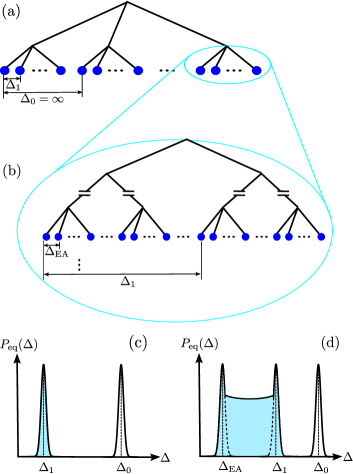
From the solution, we know that the equilibrium distribution of the order parameter, , has two peaks for (see Fig. 2) Franz and Parisi (1995); Castellani and Cavagna (2005). The first characterizes the distance between two glass configurations within a same metabasin. It is centered around , which is the typical size of this basin. The second characterizes the inter-basin distance. It is centered around , because states that belong to different metabasins are completely uncorrelated. In technical terms, this situation is described by a 1-step replica symmetry breaking (1RSB) scheme Mézard et al. (1987). Note, however, that the peak at has an exponentially small weight in , because there exists an exponentially large number of distinct glass states Castellani and Cavagna (2005). Hence, in the thermodynamic limit, everywhere in the liquid phase, i.e. even for .
II.3 Glass state following and the Gardner transition
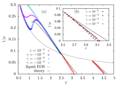
In , each equilibrium configuration at density is forever trapped into one of the exponentially many glass metabasins. The pressure of an equilibrium configuration at is given by the liquid EOS, Eq. (6), but if one compresses (or decompresses) such a configuration up (or down) to a density , the system remains within the metabasin that was initially selected. The system thus falls out of equilibrium in the sense that it cannot visit the ensemble of all possible distinct glass metabasins and thus follows an EOS different from that of the liquid.
The infinite lifetime of these glass states implies that one can adiabatically follow the EOS of a single glass state through a restricted equilibrium approach, a construction also known as state following (SF) Silvio Franz and Giorgio Parisi (1995); Barrat et al. (1997); Zdeborová and Krzakala (2010); Rainone et al. (2015). SF consists in using a first configuration that is equilibrated at initial density , and a second configuration that is in a restricted equilibrium at a different density Silvio Franz and Giorgio Parisi (1995); Barrat et al. (1997); Zdeborová and Krzakala (2010); Rainone et al. (2015). The restriction is that that second configuration must be part of the same metabasin as the first one. The state of the second configuration thus describes the evolution of the glass metabasin with . Dynamically, this process corresponds to preparing a system at equilibrium at initial density , then compressing it at density , and assuming that it is able to equilibrate inside the glass metabasin, but without escaping it. In simpler words, structural relaxations are frozen and particles only rattle inside their cages. Upon compression, these cages shrink until the jamming density, , is reached. Particles are then mechanically in contact, which makes the system mechanically rigid. In the following, we call the restricted equilibrium EOS of a given glass metabasin simply its glass EOS.
Examples of different glass EOS obtained by SF are given in Fig. 1 Rainone et al. (2015, tion). In , a compressed state under restricted equilibrium undergoes a Gardner transition at , at which point the glass metabasin subdivides into a hierarchy of sub-basins. Technically, before the Gardner transition, i.e., for , the glass metabasin is obtained by a replica symmetric SF (SF-RS) computation 333A replica symmetric SF computation is quite similar to a standard 1RSB computation., while in the Gardner phase, i.e., for , a full replica symmetry breaking SF (SF-fullRSB) computation is needed Gardner (1985); Gross et al. (1985); Mézard et al. (1987); Charbonneau et al. (2014a, b); Rainone et al. (2015). The Gardner transition is therefore akin to the spin glass transition one of the SK model, but restricted to a single glass metabasin. The high temperature phase of the SK model thus corresponds to a simple glass metabasin for while the low temperature phase corresponds to a fractured and marginal metabasin for . Note that we here complement the SF-RS computation of Ref. Rainone et al. (2015) with a SF-fullRSB computation, in order to obtain the complete EOS reported in Fig. 1. The SF-fullRSB equations are similar to the ones reported in Ref. Charbonneau et al. (2014b), but the full details of this work are given elsewhere Rainone et al. (tion).
Following a glass state in restricted equilibrium gives for a distribution that has a single peak at . Note that because the system is confined to a single glass basin, the peak at is absent. At the glass basin fractures in a SF-fullRSB structure, and correspondingly the single peak in the distribution fractures into two peaks centered around and , connected by a wide continuous band (see Fig. 2 and Mézard et al. (1987)). Here, is the typical size of the innermost sub-basins at the lowest hierarchical level, and is the typical distance between the outermost sub-basins, i.e., the size of the metabasin. For the same reason as above, does not show the peak.
Because the cage order parameter changes continuously at , the Gardner transition is a continuous critical transition Gardner (1985); Gross et al. (1985). The Gardner phase is also marginally stable, in the sense that a zero mode is always present in the stability matrix of the free energy Mézard et al. (1987). Because jamming is located within the Gardner phase, its marginal stability and critical scaling behaviors can consequently be obtained from a fullRSB thermodynamic calculation Charbonneau et al. (2014a, b).
II.4 Timescales
The timescales that characterize the dynamics in the different phases of the MK model are predicted based on the general correspondence between statics and dynamics in spin glasses Cugliandolo and Kurchan (1993, 1994). Here again, we only consider the system behavior in the limit . Beyond the microscopic timescale , over which dynamics is essentially ballistic, one gets the following picture.
-
•
In the liquid phase below , dynamics is characterized by two timescales: the -relaxation timescale , over which particles explore their transient cage, and a longer timescale , over which dynamics is diffusive. Both timescales are finite for , and diverge at according to the scaling predicted by mode-coupling theory (MCT) Götze (2009). We do not discuss this regime further because it is not directly related to the Gardner transition.
-
•
In the liquid phase above and in the SF-RS (simple glass) phase, the same two timescales exist: is the timescale for jumping from one glass metabasin to another, which being infinite in the thermodynamic limit properly defines the glass metabasins, and is the timescale for equilibrating within a glass metabasin, i.e., for particles to explore their cage, which is finite for but diverges upon approaching from densities above it, again following a MCT-like scaling form Götze (2009).
-
•
Upon approaching the Gardner transition, again diverges, scaling as . It does so for the exact same reason as at near the spin-glass transition of the SK model and corresponds to the critical slowing down close to a second-order phase transition.
-
•
In the Gardner phase, dynamics is described by three timescales: is the timescale for equilibrating within a single glass sub-basin (), is the timescale over which system explores the structure of the sub-basins within a given glass metabasin (), and remains the timescale for jumping from one glass metabasin to another (). To be more clear, none of these processes correspond to a simple exponential with a single timescale. Everywhere in the Gardner phase , because of the phase’s marginality. The relaxation inside a single sub-basin is thus expected to scale as a power-law in time. The exploration of sub-basins is characterized by a complex distribution of free energy barriers and relaxation times, and thus with ( is expected in the SK model Mézard et al. (1987)). Note that barriers between sub-basins are much lower than those between metabasins, hence .
Let us now situate the scheme for our work in this complex dynamic phase diagram. We are conveniently not concerned with the scalings of the MCT regime. Thanks to the planting procedure (see Sec. III.1), we are indeed able to easily generate equilibrium configurations of the MK model for arbitrary , including . These configurations are well equilibrated in a glass metabasins and therefore have an infinite (in the thermodynamic limit) and a finite . Because in this density regime, we can simply forget about its existence and consider that we are forever restricted into a given glass metabasin. From this point of view, we are in a situation similar to that of a spin glass where one is able to start at equilibrium in the paramagnetic, high temperature phase.
If we compress the system slowly enough to a final density , then equilibration within the glass metabasin is possible, because remains finite. In this situation, the system behavior is described by the SF-RS computation. To study the Gardner transition, however, we need to compress the system up to , at which diverges. Hence, upon approaching , eventually becomes larger than the simulation timescale, and equilibration (even in the restricted SF sense) becomes impossible. The system thus falls out of (restricted) equilibrium and is not described anymore by the SF computation.
For the situation is even worse both as and are infinite. The SF-fullRSB computation, which gives the restricted equilibrium properties in this regime, is only an approximation even at long (but not divergent with ) times. The situation is akin to that in the SK model where the fullRSB computation is only an approximation of the states reached dynamically at long times in the spin-glass phase. Because in this regime the planting technique does not work (it only works on the liquid line in Fig. 1), we cannot use it to study the restricted equilibrium in the Gardner phase.
In the following we will therefore present two kinds of data:
-
•
for , far enough from such that is smaller than the simulation timescale, we obtain restricted equilibrium data
-
•
for and , the system is out of (restricted) equilibrium, shows aging effects, and, at long times, we obtain states that are qualitatively similar to the SF-fullRSB ones, but not exactly equal to them.
In Sec. III we give a more precise definition of the numerical protocol we use to study these different regimes. Note that, according to the above discussion, from now on we will refer to the restricted equilibrium simply as “equilibrium”, given that we always work inside a glass metabasin.
II.5 Finite-dimensional MK model
To conclude this section, we discuss the additional effects that appear when one considers the MK model in finite dimensions, and that affect the above discussion.
From a theoretical point of view, a finite affects quantitatively the phase diagram, but to a lowest degree of approximation one can simply take the phase diagram of Fig. 1 and fix the value of (e.g. ) to obtain result for the EOS. However, there are several systematic corrections that impact the accuracy of this result.
-
•
The infinite-dimensional results are obtained within a Gaussian structure of the cage, which provides the exact results in the limit Kurchan et al. (2012). The Gaussian equations are slightly different in finite Parisi and Zamponi (2010). The corrections have the form of a series in and are quite small. For example, in one has instead of the infinite-dimensional result . These corrections are negligible and could be easily taken into account if needed.
-
•
A more important problem is the inexactitude of the Gaussian assumption for the MK model in finite dimensions. One should instead optimize the free energy over a generic cage function, but this computation is technically quite difficult. In Ref. Charbonneau et al. (2014c), however, two different cage functions were studied and found to give similar results. The corrections coming from the non-Gaussianity of the cage are thus also rather small, although they are more difficult to estimate.
-
•
In finite , cages are heterogeneous Charbonneau et al. (2014c). Carefully taking this effect into account would require a cavity calculation similar to the one performed in Ref. Charbonneau et al. (2014c), which is beyond the scope of this work, but is also likely a small correction for Charbonneau et al. (2014c).
For all these reasons, the results of Fig. 1 are only an approximation to the finite-dimensional phase diagram. In the following, we will nonetheless take the results of the simplest theoretical approximation, namely take the results of Fig. 1 and use them in , after properly rescaling the axes. We expect (and check) that the corrections are quite small. Sometimes, however, in order to take effective account of these corrections, we will further rescale the results, so as to obtain a better quantitative agreement between theory and simulation.
The most important genuinely finite-dimensional effect is hopping. As discussed in Ref. Charbonneau et al. (2014c), slightly above , particles are not perfectly confined in their cages, as one would expect based on the picture. Instead, each particle is allowed to explore a network of cages, connected by narrow pathways. Hopping consists in particles jumping between distinct cages. The corresponding time scale is finite at and thus the divergence of the relaxation time is washed away in finite . Hopping effects also change deeply the dynamics of the system with respect to the prediction, and the configurations at are not able to constrain the dynamics for infinitely-long times. Because the timescale for hopping increases quickly upon increasing both density and dimension, considering values of that are slightly above suffices. In practice, based on the analysis of Ref. Charbonneau et al. (2014c), in and for hopping is strongly suppressed, hence in that regime the mean-field, scenario should apply reasonably well.
III Numerical Approach
In this section, we provide the numerical details used in the simulations of the glass states of the MK model.
III.1 Planting
An important algorithmic advantage of the MK model is that planting can be used to generate equilibrium liquid configurations at any Krzakala and Zdeborová (2009); Charbonneau et al. (2014c). This procedure sidesteps the tedious and time-consuming work of first preparing dense equilibrium configurations, as would be needed for typical glass formers, such as HS. The basic idea is to switch the order in which initial particle positions and random shifts are determined. One first chooses the particle positions independently and uniformly in the volume , and then for each particle pair one chooses a random shift uniformly under the sole constraint that the two particles should not overlap, which is quite straightforward to satisfy. As long as the quenched and the annealed averages of the free energy are the same (see Ref. Krzakala and Zdeborová (2009) for a more detailed discussion), a planted state is a true equilibrium state and automatically satisfies the liquid EOS, Eq. (6). This condition is met along the replica symmetric phase for , where is the Kauzmann point at which the configurational entropy vanishes Parisi and Zamponi (2010); Mari and Kurchan (2011). Because in the MK model Mari and Kurchan (2011), planting a liquid configuration is thus possible at any density, which dramatically reduces the computational cost of the initial equilibration.
In our notation, a given and defines a sample. A sample thus identifies a given system (defined by ) and, for this system, one of its glass metabasins (selected by ).
III.2 Molecular dynamics (MD) simulations
We use event-driven molecular dynamics (MD) to simulate MK particles in Skoge et al. (2006); Charbonneau et al. (2014c). Periodic boundary conditions with the minimum image convention are implemented on the shifted distances . Time is expressed in units of , where the particle mass and diameter as well as the inverse temperature are set to unity. Systems consist of particles unless otherwise specified. This system size is large enough to contain a first full shell of neighbors around each particle, and to keep the periodic boundary effects on caging to a minimum Charbonneau et al. (2014c). Finite-size effects are studied for some of the observables for the initial liquid density (see Sec. IV.2).
To simulate SF, for a given sample, we start from the planted equilibrium configuration at a packing fraction , and grow the spheres following the Lubachevsky-Stillinger algorithm Donev et al. (2005); Skoge et al. (2006) at constant growth rate , unless otherwise specified, up to a desired . Once compression is stopped at the target density, the origin of time is set. We will thus typically (although not always) define the waiting time , as the time that has elapsed since the end of the compression. From that moment on we start measuring observables, keeping density and temperature (and thus energy) constant. Note that because is finite and rather small, part of the equilibration happens already during compression, so provided we are not too close to the system is stationary at all (we come back on this point later). This procedure is repeated over samples in order to average over thermal and quenched disorders. Errors are computed using the jack-knife method Amit and Martin-Mayor (2005). Depending on the statistical convergence of the different observables, is varied from 500 to 75,000, as specified in the discussion of the various measurements.
III.3 Observables
The pressure evolution along SF is reasonably well described by a free-volume EOS
| (8) |
where is a fitting parameter. Fitting Eq. (8) to the compression results provides an estimate of (see Table 2). If a sufficiently small is chosen, no aging is observed in the pressure, and using slower compression rates gives only negligible corrections to the glass EOS (see Fig. 3). Interestingly, upon decompression, the state follows the same EOS up to a threshold density at which it melts into a liquid phase. This phenomenon has been recently predicted by the theory Mariani et al. (2015); Rainone et al. (2015), and observed numerically in simulated ultrastable glasses Singh et al. (2013); Hocky et al. (2014).
To obtain more structural information about the free energy landscape, we also simulate a cloning procedure. The approach consists of taking two exact copies (clones) and of the same planted configuration at , and assigning them different initial velocities, randomly drawn from the Maxwell–Boltzmann distribution. These two copies are then independently compressed up to , before measuring the mean-squared distance between them
| (9) |
where and are the positions of particle at time in clones and , respectively. Although the two clones start from the same initial configuration, their compression histories are different once is reached.
The detailed behavior of the clones will be discussed in Sec. IV.1, but let us explain here briefly why the cloning procedure is useful to detect the Gardner transition. In the SF-RS phase, the two clones are uncorrelated in the glass basin and converges quickly (on a time scale if the two clones are not sufficiently well equilibrated along the compression) to the equilibrium value . Hence in the SF-RS phase. By contrast, if the end point of the compression falls within the SF-fullRSB (or Gardner) phase, clones most likely fall into different sub-basins. Their mean square distance can then be described by a non-trivial time-dependent probability distribution, , that depends on the way sub-basins are sampled. Calculating these weights is difficult, because the two clones are generally out of equilibrium. Because the probability that the two clones fall in the same state is very small, however, and therefore for all . Hence, in the Gardner phase at all is strictly larger than the long-time limit of the MSD. The long time limit of , being zero in the SF-RS phase and non-zero in the SF-fullRSB phase, thus provides an order parameter for the Gardner transition.
IV Detecting the Gardner transition
In this section, we describe different means of detecting the Gardner transition through numerical simulations designed to follow the evolution of glassy states. Let us stress once again that the aim of this work is to understand, in a controlled setting, how well numerical simulations and experiments can detect the Gardner transition. We can therefore test different strategies to understand their advantages and limitations, and use the analytical results to assess the quality of the numerical results. Based on the discussion in Sec. II, we follow two complementary approaches. The first is based on dynamics. From the long-time dependence of the mean square displacement, we determine , whose divergence in the glass metabasin signals the Gardner transition. The second is based on the properties of the distribution function , which becomes non-trivial in the Gardner phase. We investigate different moments of this distribution to detect signatures of the transition.
IV.1 Dynamics
As discussed in Sec. II.4, the Gardner transition is a second order phase transition associated with a diverging characteristic relaxation time that controls the dynamics of the MSD. To detect this relaxation time we make use of the following observables already briefly discussed in Sec. III. Recall that the origin of time is set at the end of the compression when a given final density is reached.
IV.1.1 Definition of the relevant observables
We define the MSD between two configurations at different times:
| (10) |
and the MSD between two different clones
| (11) |
From these two instantaneous quantities we can define different observables. The statistical average (over compressions and samples) gives
| (12) |
and we define
| (13) |
We also define a time-dependent caging susceptibility as the normalized variance of the MSD
| (14) |
and its counterpart of cloned configurations
| (15) |
In the SF-RS phase in restricted equilibrium, i.e., at large enough and , gives back Eq. (7), while does not depend on time. In this case
| (16) |
gives the average cage radius of the glass basin. Similarly, and , where
| (17) |
is the average susceptibility of the glass basin. Finally, note that based on Eq. (16), we have
| (18) |
By contrast, in the SF-fullRSB phase, equilibrium is not reached even for very large (recall that we do not consider here times that are comparable to ). Therefore, remains non-zero even for large and , which makes the long time limit of a dynamic order parameter for the Gardner transition.
IV.1.2 Qualitative change in caging and susceptibility
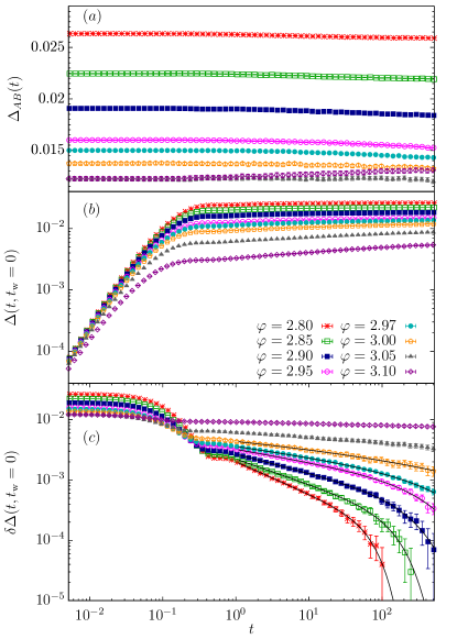
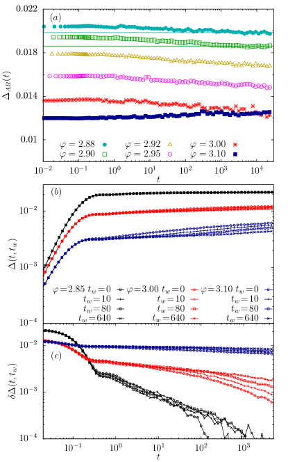
Figure 4 shows the time dependence of , and for , averaged over to from the lowest and highest , respectively. Both and are observed to behave slightly differently below and above ( for , a more precise estimate is obtained below). For , first (and up to a microscopic time ) grows quickly because of the ballistic motion of particles Charbonneau et al. (2014c) and then more slowly in the relaxation regime, before eventually reaching the plateau that defines the cage size. This plateau coincides with the (almost time-independent) results for , as is qualitatively expected for a system in a SF-RS phase. For , the situation is a bit more convoluted. As discussed above, beyond the Gardner transition each of the original metabasins is expected to subdivide into a hierarchical distribution of glassy states. Equilibration within the glass metabasin is now, however, impossible, and we thus observe that depends on time for all observable times while remains always strictly smaller than and never reaches a plateau. Correspondingly does not decay to zero.
In Fig. 5, we select a few densities and consider the evolution of over much larger times than in Fig. 4 as well as the dependence of on both and . Note that these data are averaged over many fewer samples, . We consider the detailed behavior of these two quantities:
-
•
In general, (Fig. 5a) should correspond to the average distance between configurations restricted to within a given metabasin, but for the basins are sampled with non-equilibrium weights, and hence slowly drifts. For , we indeed observe that once , reaches a stationary value. Upon approaching and for , however, is becomes so large that the drift of persists at all simulated times. Note that the drift can be positive or negative, depending on density.
-
•
The behavior of (Fig. 5b) is naturally described as a function of for fixed . Below (e.g., for ), is independent of and behaves as in Fig. 4. Beyond (e.g., for ), however, the system is initially trapped into a sub-basin, and thus grows until reaching a plateau corresponding to the size of the sub-basin, , for . For , the system can explore the structure of sub-basins, hence keeps increasing, and no clear first plateau can be detected. A second plateau should be reached in the limit , when the metabasin is fully explored, but this regime is here beyond computational reach. The timescale indeed increases with Cugliandolo and Kurchan (1993, 1994), as is clearly visible in Fig. 5, where the drift shifts towards larger times upon increasing . Note that in the limit , should diverge for , but a finite acts as a cutoff and should instead saturate to a value for large .
-
•
In the Gardner phase for all accessible times . Therefore, although goes to zero at large times for , for it does not fully decay in the accessible regime (for all ) and instead converges to a plateau (Fig. 5c). Note also that the evolution of with increasing density is qualitatively identical to that of the overlap with decreasing temperature in spin glasses, as reported in Ref. (Ogielski, 1985, Fig. 8) (compare also to Fig. 4c). These results further support the strong analogy between the Gardner and the spin-glass transitions.
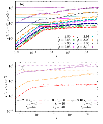
The dynamical behavior of the caging susceptibility is qualitatively similar that of the MSD (Fig. 6). As for the cage order parameters, in the SF-RS phase (for ) the two susceptibilities become identical in the long time limit, i.e., . By contrast, in the SF-fullRSB phase (for ), on a timescale , we generally observe that . Note that the magnitude of the susceptibility increases by more than a decade in the density range considered here, which is a clear signature of the Gardner transition. A detailed analysis of this increase is discussed in Sec. IV.2.3.
IV.1.3 Computation of timescales
Based on the qualitative picture of the dynamics presented above, we now attempt a more quantitative analysis based on the classic work of Ogielski on spin glasses Ogielski (1985) and its recent extension to the study of the dynamical transition in the Edwards-Anderson model under an external field Baity-Jesi et al. (2014a). The idea consists in obtaining a relaxation timescale from the decay of (Fig. 4c). Note, however, that this scheme is only well defined in the SF-RS phase, where equilibrium can be reached and Eq. (18) holds. In the SF-fullRSB phase, does not decay to zero and evolves continuously over a broad range of time scales. Extracting a single timescale is then not so straightforward. We will focus in the following on the data for , for which we have more statistics. For , these data are also representative of all .
In order to facilitate the numerical analysis, we make use of analytical results. According to the general theory of critical glassy dynamics developed in Refs. Sompolinsky and Zippelius (1982); Caltagirone et al. (2012); Parisi and Rizzo (2013), upon approaching the Gardner point in (restricted) equilibrium from the SF-RS phase, hence when does not depend on , one has:
| (19) |
where and the function is such that while decays exponentially. Here the exponents and are related to the so-called MCT exponent parameter by the relation
| (20) |
The parameter can be computed analytically within the replica method by analizing the cubic terms of the replica action Caltagirone et al. (2012); Parisi and Rizzo (2013); Kurchan et al. (2013). The results of this computation are reported in Table 1 (details are given in Refs. Rainone et al. (tion)).
In order to estimate , we fit the results for using an empirical form that has been used for spin glasses Ogielski (1985); Baity-Jesi et al. (2014a), which gives
| (21) |
where the parameters , and depend on , , and offers a first estimate of . Note that we fit the exponent instead of using the analytical result, because the critical regime over which the exponent coincides with is narrow and away from the effective exponent is quite different (see Ref. (Ogielski, 1985, Fig. 12)). With this choice all the fits are very good, as reflected by the Pearson per degree of freedom (d.o.f.) 444Recall that , where is the numbers of times and , is the error of , and is the fitting function, Eq. (21) being much less than 1 (examples of the quality of the fit are given in Fig. 4c). As approaches for a given , is expected to diverge as
| (22) |
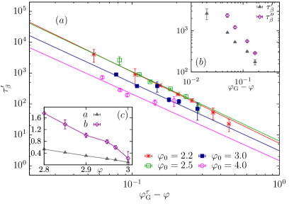
In order to obtain a more constrained value of , we fix the exponent to its analytic value given in Table 1 and only fit and the prefactor. This time the fits are not excellent, with values of of the order of 1 or larger (see Fig. 7). The results for are reported in Table 2.
| 4.8 | 4.8 | 0.7027 | 3.069 |
|---|---|---|---|
| 4.9 | 5.34 | 0.5607 | 2.651 |
| 5 | 5.64 | 0.5091 | 2.547 |
| 5.25 | 6.18 | 0.4378 | 2.427 |
| 5.5 | 6.61 | 0.3938 | 2.363 |
| 6 | 7.33 | 0.3398 | 2.295 |
| 6.667 | 8.16 | 0.2957 | 2.245 |
| 7 | 8.54 | 0.2801 | 2.228 |
| 8 | 9.63 | 0.2469 | 2.194 |
| 10.667 | 12.36 | 0.2042 | 2.154 |
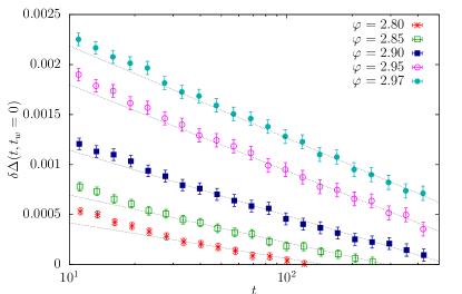
An alternative estimate of can be obtained from the logarithmic scaling of at long times (see Fig. 8). For , the fitting form
| (23) |
with a density-dependent constant gives Baity-Jesi et al. (2014a). Comparing and suggests that the divergence of the two timescales is compatible with a same and a very similar power-law exponent (see Fig. 7b). The insensibility of the estimator of to its precise definition adds support to our claim that the observed divergence is due to a true thermodynamic transition. Also, we repeated the analysis for with very similar results.
To conclude the discussion, note that the results for and at low densities, i.e., , may be affected by hopping (Sec. II.5 and Charbonneau et al. (2014c)). In these systems the timescale for leaving a metabasin (albeit only through local hopping processes) is comparable to even near . The estimate of in this regime is therefore subject to a larger error, which explains the bigger difference between and other estimates (Table 2). For the limit case , we do not even attempt to fit the data because no clear power-law regime can be distinguished. By contrast, for , hopping is negligible on the timescales achieved numerically.
IV.2 Static functions
As we have shown in Sec. IV.1, at the Gardner transition two-clones observables such as become different from the long-time limit of dynamic observables such as . In this subsection, we thus estimate the location of the Gardner transition using an approach based on the study of two-clone static observables. These observables are static because, as we showed in Sec. IV.1, they are time independent for . We can thus arbitrarily choose any to compute them. Here, we choose , such that , which we abbreviate below as and . We use a similar notation for all other observables unless otherwise specified.
IV.2.1 Average mean square displacement
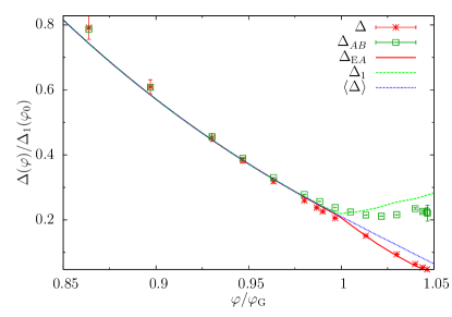
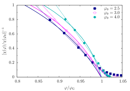
We consider the averages of and and compare them with the theoretical SF results (see Fig. 9 for ). In order to take into account the corrections discussed in Sec. II.5, both the numerical and the theoretical datasets have been rescaled. For the vertical axis, we rescale the results to , which is known both in theory and in simulation, such that both datasets are equal to 1 for . For the horizontal axis, we rescale to with the theoretical for the SF-RS curve (Table 1) and a fit factor for the numerical results (Table 2). Figure 9 clearly shows the difference between the two expected regimes (Sec. II.3): for , we obtain , while for , we obtain and , and hence . Although at short times we observe , on much longer timescales we expect to evolve slowly towards its equilibrium value , which is however only approached for that diverge with .
IV.2.2 Probability distribution functions
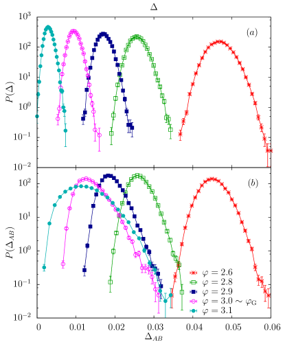
We next consider the probability distribution function (pdf) of the cage order parameters by computing and for each sample and constructing the histogram over samples. Note that because is the mean square displacement restricted to a single sub-basin and the waiting time is fairly short, its distribution represents in the SF-RS phase, and only the peak around in the SF-fullRSB phase (see Fig 2).
Figure 10 shows and for calculated from – 75,000 samples. The shape of is Gaussian-like at all , and its mean value monotonically decreases with increasing . The shape of , however, changes considerably over that same regime. For , it is Gaussian and analogous to that of , but near it develops an exponential tail akin to a Gumbel distribution. If is further increased, then becomes broader, which is consistent with the theoretical expectation (see Fig. 2).
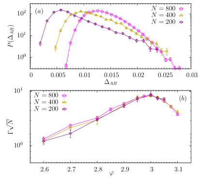
The development of an exponential tail at the critical point has been observed and studied for spin glasses in a field Parisi and Ricci-Tersenghi (2012); Baity-Jesi et al. (2014b). The effect is thought to be due to disorder. Whereas the results for most samples fall within Gaussian fluctuations around a given mean value, a few rare samples have much larger than the mean, giving an exponential tail to the distribution. The smaller the system, the stronger the effect (Fig. 11). These rare fluctuations are hypothesized to originate from the sample-to-sample fluctuations of the critical point Parisi and Ricci-Tersenghi (2012), which then translates into significant sample-to-sample fluctuations of some of the measured observables. We come back to this point in Sec. IV.3.
The connection between the changing shape of the distribution and criticality suggests that we can determine the critical transition from alone. We propose below two alternative procedures for detecting the Gardner transition using standard moments of the distribution.
IV.2.3 Caging susceptibility
We first define a caging susceptibility from the normalized variance of
| (24) |
where the denominator corrects for the fact that changes with . As in the vicinity of any critical point, the susceptibility is expected to diverge as
| (25) |
where the critical exponent 1 is due to the fact that the MK model is mean-field in nature.
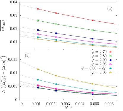
.
The definition of involves taking the quotient of two quantities that both suffer from strong finite-size corrections. In order to control for this effect we study the behavior of both terms as function of (Fig. 12). The denominator, , behaves as a regular series in , decreases smoothly with , and eventually saturates above the Gardner point. The numerator, has, however, a more complex behavior. While it follows a nearly behavior for with a small dependence on , it grows significantly faster both with and for . We attempt to extract the value of both quantities at the thermodynamic limit using a second-order polynomial fit in , even though for the estimate of obtained in this way is not reliable and larger systems would be needed to obtain a better extrapolation.
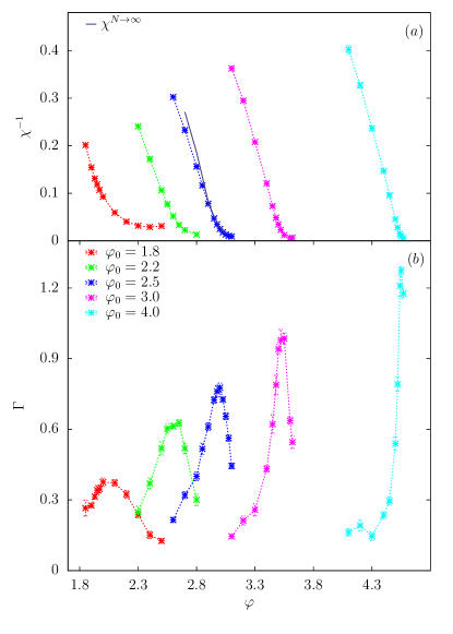
The results for the susceptibility for are reported in Fig. 13a for different values of (and thus ). For we also include obtained using the extrapolations of Fig. 12. The comparison suggests that although the finite-size effects in both and are still very strong for this system size, the determination of is fairly well controlled, at least for .
The numerical data in Fig. 13a suggest a roughly linear behavior of for all except , where the spacing between and is narrowest, and where hopping most likely obfuscates the critical regime (see Fig. 16). For the other , we estimate the Gardner transition by fitting Eq. (25) in the region (Table 2 and Fig. 16).
In Fig. 14 we compare the numerical results with the theoretical predictions. Note, however, that the theoretical curves do not correspond to the full value, but only include the leading divergent term, namely the inverse of the replicon eigenvalue (see Charbonneau et al. (2014b); Rainone et al. (tion) for details). As discussed for Fig. 9, both the theoretical and numerical datasets are also rescaled. The vertical axis is normalized to 1 at , while the horizontal axis is scaled to , using the theoretical values in Table 1 and the fit values for the numerics (Table 2). Interestingly, the theoretical curves are not linear over the whole density regime. They instead bend towards , before vanishing linearly, but only in a fairly small region around . The linear scaling observed in the simulation data is thus likely due to finite-size effects. The numerical estimates of obtained from the linear fit of the whole set of data for thus slightly overestimate the true transition point. Yet the effect is quite small – approximately , based on Fig. 14. For and above, we observe that finite-size effects dominate the numerical determination of , which remains finite instead of diverging.
IV.2.4 Caging skewness
Near the Gardner transition, large sample-to-sample fluctuations give rise to a strong exponential tail in . This effect can be quantified by the skewness of the distribution
| (26) |
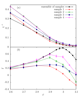
Recall that the skewness is a measure of a distribution’s asymmetry and that a Gaussian distribution would have . Sample-to-sample fluctuations are expected to be maximal at the critical point (see Sec. IV.3), which provides an estimate of the Gardner transition, (see Fig. 13b and Table 2). For all , we see that is very close to the fitted divergence of the susceptibility, . Finite-size analysis further shows that the rescaled skewness, , collapses the data for different (Fig. 11). The peak of is thus expected to persist all the way to the thermodynamic limit, consistently with comparable observations in spin-glass models Parisi and Ricci-Tersenghi (2012).
IV.3 Sample-to-sample fluctuations
We have assumed above that the abnormal behavior of around the Gardner transition is due to sample-to-sample fluctuations, and we further motivate this hypothesis here. Recall that in our notation a sample is defined by a given configuration and a set of random shifts (see Sec. III.1). To compute the moments and of each sample, we perform independent clonings for each sample. In Fig. 15, the data for the ensemble of samples (same data as in Fig. 13) are compared with those of four individual samples. We note that the density evolution of for the individual samples can have a very different behavior from the ensemble one. In particular, a peak around is generally not seen.
Sample-to-sample fluctuations have a smaller effect on (Fig. 15). While the magnitude and the critical density exhibit some fluctuations, they all display a divergence similar to that of Eq. (25). Because each realization of disorder corresponds to different SF-RS metabasins, our results suggest that the metabasins themselves have slightly different properties. In particular, they exhibit different , which is likely the physical origin of the exponential tail of and thus of its anomalous skewness Parisi and Ricci-Tersenghi (2012).
V Summary of results
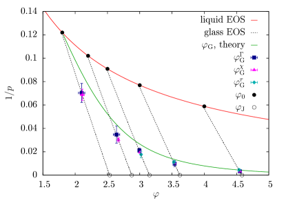
The Gardner transition at was independently and quantitatively identified from: (i) the power-law divergence of the characteristic time in Fig. 7, (ii) the linear vanishing of the inverse susceptibility in Fig. 13a, and (iii) the maximum of the skewness in Fig. 13b. Table 2 contains these results and Figure 16 presents them in a phase diagram. The different estimates of are generally quantitatively consistent with each other and qualitatively consistent with the mean-field SF results from .
The agreement with the mean-field calculation improves with density, likely because the Gaussian caging approximation used in the theory becomes a better approximation at higher densities Kurchan et al. (2012); Charbonneau et al. (2014c). A couple of reasons underlie the discrepancy between numerical estimates and theory in the vicinity of . First, caging becomes imperfect at such low densities, which allows particles to hop between neighboring cages on a timescale comparable with the simulation time Charbonneau et al. (2014c). Hopping thus affects the dynamics of the system ( and ) and also transforms the transitions (at either or ) in crossovers. Second, because is expected to converge to upon approaching the dynamical glass transition (see Figs. 1 and 16), the critical regime becomes too small to make any fit to a critical power-law scaling.
| 1.8 | 2.10(5) | 2.11(3) | – | – | 2.534(3) |
| 2.2 | 2.64(5) | 2.670(11) | 2.72(4) | – | 2.876(4) |
| 2.5 | 2.995(15) | 3.006(6) | 3.06(2) | 2.96 | 3.151(3) |
| 3.0 | 3.54(2) | 3.537(3) | 3.554(17) | 3.49 | 3.622(5) |
| 4.0 | 4.550(12) | 4.551(5) | 4.57(2) | 4.48 | 4.584(4) |
In addition to (i)-(iii), a more indirect way (iv) to determine has been reported in Fig. 9 by comparing the density evolution of the cage order parameters with the theoretical predictions in . However, while the effect is qualitatively (and visually) clear, obtaining a quantitative measure of from this approach is somewhat ill-defined. For one also should treat results with caution. As discussed above, because of the finite-size and out-of-equilibrium nature of the system, the value of drifts with time as different sub-basins are explored. Because in practice we evaluate at a relatively short time (Sec. IV.2), we likely obtain a reasonable estimate of the size of a single sub-basin, but this procedure is also somewhat uncontrolled.
Overall, we find that the most reliable way to determine is the divergence of (procedure (i)). This effect is clearly the most spectacular signature of the transition, and sample-to-sample fluctuations do not much affect its detection (Fig. 15). Interestingly, because is almost independent of time, one can determine reliably using at short times, as we did in this paper. Once is determined in this way, a useful test is to check that this value is consistent with the behavior of and , as in Fig. 9. Procedure (iii), i.e. finding the maximum of the skewness, requires averaging over a large number of samples which will surely be difficult in numerical simulations of realistic models of glasses as well as in experiments, where producing equilibrium configurations is extremely difficult. Procedure (i), i.e. the divergence of , is also difficult because the determination of is subject to some ambiguity, but the study of the dynamics is useful because aging effects are manifest for (Fig. 5). Procedure (iv) is used here as a consistency check with the theory, rather than a method to detect .
VI Conclusions
The Gardner transition separates a stable glass metabasin at low densities (high temperatures) from a complex hierarchy of marginally stable sub-basins, at high densities (low temperatures). Its existence, which is proven in mean-field glass models Gardner (1985); Gross et al. (1985), has deep consequences on the low-temperature physics of glasses and on jamming Charbonneau et al. (2014a, 2015). It is therefore extremely interesting to check whether such a transition exists in realistic models of glasses and in experiments.
In this work we have investigated and compared several numerical procedures for detecting the Gardner transition in the MK model, which belongs to the universality class of mean-field spin glasses while remaining fairly close to realistic glass formers Mari and Kurchan (2011). We have presented three independent approaches for locating the transition, all of which show that the transition exists and is found in a region that is roughly consistent with theoretical predictions. We have discussed the advantages and drawbacks of each of these strategies and the importance of finite-size effects.
This work paves the way for studying the Gardner transition in more realistic numerical models of glasses, where the very existence of the Gardner transition is debated Urbani and Biroli (2015). Our approach is also suitable to be reproduced in experiments. SF, for instance, corresponds to a straightforward annealing, and some of the observables should be readily available through standard microscopy or scattering techniques.
One key hurdle to generalizing our methodology to other systems is the need to equilibrate, without planting (and thus through slow annealing), a glass state well above the (avoided) dynamic glass transition. To follow adiabatically a glass state, one should be able to prepare initial configurations such that the -relaxation time is very large (), so that the SF experiment can be performed on time scale , as discussed in Sec. II.4. For numerical simulations this requirement can be particularly computationally onerous, but it may be more easily achievable in experimental systems, where longer timescales can typically be reached. In particular, it would be very interesting to investigate the existence of the Gardner transition in ultrastable glasses that can be prepared through vapor deposition and have an extremely large Singh et al. (2013); Hocky et al. (2014); Swallen et al. (2007); Parisi and Sciortino (2013). In experiments, the bigger challenge would be to substitute the cloning procedure with a (potentially very) large number of experimental replicates.
Finite-dimensional non-mean-field glass formers display features that are not observable in the MK model. In particular, we expect a diverging length scale to be associated with the Gardner transition in these systems. This length scale is expected to capture static heterogeneity, which represents the spatial inhomogeneity of cage sizes around and above . In principle, this kind of static heterogeneity should be different from both the dynamic heterogeneity around the dynamic glass transition, and the heterogeneity close to jamming, which is related to soft relaxation modes Brito and Wyart (2009). Understanding the relevance of marginal stability for glassy dynamics, and the relation with the ideas of Ref. Brito and Wyart (2009), would open a new window on the property of low-temperature glasses.
Acknowledgements.
We wish to thank L. Berthier, O. Dauchot, W. Kob, J. P. Bouchaud, G. Biroli, J. Kurchan, S. Franz, T. Rizzo, F. Ricci-Tersenghi, and M. Wyart for very useful discussions, and especially P. Urbani and H. Yoshino for collaborating with two of us in the theoretical part of this project Rainone et al. (2015, tion). P.C. acknowledges support from the Alfred P. Sloan Foundation and NSF support No. NSF DMR-1055586. B.S. acknowledges the support by MINECO (Spain) through research contract No. FIS2012-35719-C02. The research leading to these results has received funding from the European Research Council under the European Union’s Seventh Framework Programme (FP7/2007-2013)/ERC grant agreement no. [247328].References
- Berthier and Biroli (2011) L. Berthier and G. Biroli, Rev. Mod. Phys. 83, 587 (2011).
- Cavagna (2009) A. Cavagna, Physics Reports 476, 51 (2009).
- Liu and Nagel (1998) A. J. Liu and S. R. Nagel, Nature 396, 21 (1998).
- Kamien and Liu (2007) R. D. Kamien and A. J. Liu, Phys. Rev. Lett. 99, 155501 (2007).
- Parisi and Zamponi (2010) G. Parisi and F. Zamponi, Rev. Mod. Phys. 82, 789 (2010).
- Donev et al. (2005) A. Donev, S. Torquato, and F. H. Stillinger, Phys. Rev. E 71, 011105 (2005).
- Skoge et al. (2006) M. Skoge, A. Donev, F. H. Stillinger, and S. Torquato, Phys. Rev. E 74, 041127 (2006).
- Silbert et al. (2006) L. E. Silbert, A. J. Liu, and S. R. Nagel, Phys. Rev. E 73, 041304 (2006).
- Chaudhuri et al. (2010) P. Chaudhuri, L. Berthier, and S. Sastry, Phys. Rev. Lett. 104, 165701 (2010).
- Hermes and Dijkstra (2009) M. Hermes and M. Dijkstra, arXiv.org:0903.4075 (2009).
- Charbonneau et al. (2011) P. Charbonneau, A. Ikeda, G. Parisi, and F. Zamponi, Phys. Rev. Lett. 107, 185702 (2011).
- Ikeda et al. (2012) A. Ikeda, L. Berthier, and P. Sollich, Phys. Rev. Lett. 109, 018301 (2012).
- Ikeda et al. (2013) A. Ikeda, L. Berthier, and P. Sollich, Soft Matter 9, 7669 (2013).
- Kurchan et al. (2013) J. Kurchan, G. Parisi, P. Urbani, and F. Zamponi, J. Phys. Chem. B 117, 12979 (2013).
- Charbonneau et al. (2014a) P. Charbonneau, J. Kurchan, G. Parisi, P. Urbani, and F. Zamponi, Nat. Comm. 5, 3725 (2014a).
- Charbonneau et al. (2014b) P. Charbonneau, J. Kurchan, G. Parisi, P. Urbani, and F. Zamponi, J. Stat. Mech. Theor. Exp. 2014, P10009 (2014b).
- Rainone et al. (2015) C. Rainone, P. Urbani, H. Yoshino, and F. Zamponi, Phys. Rev. Lett. 114, 015701 (2015).
- Gardner (1985) E. Gardner, Nuclear Physics B 257, 747 (1985).
- Gross et al. (1985) D. J. Gross, I. Kanter, and H. Sompolinsky, Phys. Rev. Lett. 55, 304 (1985).
- Montanari and Ricci-Tersenghi (2003) A. Montanari and F. Ricci-Tersenghi, Eur. Phys. J. B 33, 339 (2003).
- Montanari and Ricci-Tersenghi (2004) A. Montanari and F. Ricci-Tersenghi, Phys. Rev. B 70, 134406 (2004).
- Rizzo (2013) T. Rizzo, Phys. Rev. E 88, 032135 (2013).
- Mézard et al. (1987) M. Mézard, G. Parisi, and M. A. Virasoro, Spin glass theory and beyond (World Scientific, Singapore, 1987).
- Note (1) The Gardner transition is akin to that of the SK model in presence of a random magnetic field, because the system is confined in a given glass metabasin and the self-induced disorder characteristic of this glass metabasin acts as a self-induced “external” random field. At the mean-field level, this distinction does not make any difference, but the presence of a random field is important in finite dimensions Urbani and Biroli (2015).
- Lerner et al. (2013) E. Lerner, G. During, and M. Wyart, Soft Matter 9, 8252 (2013).
- Charbonneau et al. (2015) P. Charbonneau, E. I. Corwin, G. Parisi, and F. Zamponi, Phys. Rev. Lett. 114, 125504 (2015).
- Müller and Wyart (2015) M. Müller and M. Wyart, Annu. Rev. Condens. Matter Phys. (2015).
- Wyart et al. (2005) M. Wyart, S. Nagel, and T. Witten, Europhysics Letters 72, 486 (2005).
- Urbani and Biroli (2015) P. Urbani and G. Biroli, Phys. Rev. B 91, 100202 (2015).
- Binder and Young (1986) K. Binder and A. P. Young, Rev. Mod. Phys. 58, 801 (1986).
- Baños et al. (2010) R. A. Baños, A. Cruz, L. A. Fernandez, J. M. Gil-Narvion, A. Gordillo-Guerrero, M. Guidetti, A. Maiorano, F. Mantovani, E. Marinari, V. Martin-Mayor, J. Monforte-Garcia, A. M. Sudupe, D. Navarro, G. Parisi, S. Perez-Gaviro, J. J. Ruiz-Lorenzo, S. F. Schifano, B. Seoane, A. Tarancon, R. Tripiccione, and D. Yllanes, J. Stat. Mech. Theor. Exp. 2010, P06026 (2010).
- Mari and Kurchan (2011) R. Mari and J. Kurchan, J. Chem. Phys. 135, 124504 (2011).
- Mari et al. (2009) R. Mari, F. Krzakala, and J. Kurchan, Phys. Rev. Lett. 103, 025701 (2009).
- Charbonneau et al. (2014c) P. Charbonneau, Y. Jin, G. Parisi, and F. Zamponi, Proc. Natl. Acad. Sci. U.S.A. 111, 15025 (2014c).
- Kraichnan (1962) R. H. Kraichnan, J. of Math. Phys. 3, 475 (1962).
- Krzakala and Zdeborová (2009) F. Krzakala and L. Zdeborová, Phys. Rev. Lett. 102, 238701 (2009).
- Rainone et al. (tion) C. Rainone, P. Urbani, H. Yoshino, and F. Zamponi, (in preparation).
- Note (2) If one considers instead the dynamics starting from an out-of-equilibrium initial condition, then the system is able to equilibrate for while aging effects, which persist for infinite times, are observed for Cugliandolo and Kurchan (1993); Castellani and Cavagna (2005).
- Franz and Parisi (1995) S. Franz and G. Parisi, J. Phys. I 5, 1401 (1995).
- Castellani and Cavagna (2005) T. Castellani and A. Cavagna, J. Stat. Mech. Theor. Exp. 2005, P05012 (2005).
- Silvio Franz and Giorgio Parisi (1995) Silvio Franz and Giorgio Parisi, J. Phys. I France 5, 1401 (1995).
- Barrat et al. (1997) A. Barrat, S. Franz, and G. Parisi, Journal of Physics A: Mathematical and General 30, 5593 (1997).
- Zdeborová and Krzakala (2010) L. Zdeborová and F. Krzakala, Phys. Rev. B 81, 224205 (2010).
- Note (3) A replica symmetric SF computation is quite similar to a standard 1RSB computation.
- Cugliandolo and Kurchan (1993) L. F. Cugliandolo and J. Kurchan, Phys. Rev. Lett. 71, 173 (1993).
- Cugliandolo and Kurchan (1994) L. Cugliandolo and J. Kurchan, Journal of Physics A: Mathematical and General 27, 5749 (1994).
- Götze (2009) W. Götze, Complex dynamics of glass-forming liquids: A mode-coupling theory, Vol. 143 (Oxford University Press, USA, 2009).
- Kurchan et al. (2012) J. Kurchan, G. Parisi, and F. Zamponi, J. Stat. Mech. Theor. Exp. 2012, P10012 (2012).
- Amit and Martin-Mayor (2005) D. J. Amit and V. Martin-Mayor, Field theory, the renormalization group, and critical phenomena, Vol. 3rd ed (World Scientific Singapore, 2005).
- Mariani et al. (2015) M. S. Mariani, G. Parisi, and C. Rainone, Proceedings of the National Academy of Sciences 112, 2361 (2015).
- Singh et al. (2013) S. Singh, M. D. Ediger, and J. J. de Pablo, Nat. Mater. 12, 139 (2013).
- Hocky et al. (2014) G. M. Hocky, L. Berthier, and D. R. Reichman, J. Chem. Phys 141, 224503 (2014).
- Ogielski (1985) A. T. Ogielski, Phys. Rev. B 32, 7384 (1985).
- Baity-Jesi et al. (2014a) M. Baity-Jesi, R. A. Baños, A. Cruz, L. Fernandez, J. Gil-Narvion, A. Gordillo-Guerrero, D. Iñiguez, A. Maiorano, F. Mantovani, E. Marinari, et al., Phys. Rev. E 89, 032140 (2014a).
- Sompolinsky and Zippelius (1982) H. Sompolinsky and A. Zippelius, Phys. Rev. B 25, 6860 (1982).
- Caltagirone et al. (2012) F. Caltagirone, U. Ferrari, L. Leuzzi, G. Parisi, F. Ricci-Tersenghi, and T. Rizzo, Phys. Rev. Lett. 108, 085702 (2012).
- Parisi and Rizzo (2013) G. Parisi and T. Rizzo, Phys. Rev. E 87, 012101 (2013).
- Note (4) Recall that , where is the numbers of times and , is the error of , and is the fitting function, Eq. (21\@@italiccorr).
- Parisi and Ricci-Tersenghi (2012) G. Parisi and F. Ricci-Tersenghi, Philos. Mag. 92, 341–352 (2012).
- Baity-Jesi et al. (2014b) M. Baity-Jesi, R. Baños, A. Cruz, L. Fernandez, J. Gil-Narvion, A. Gordillo-Guerrero, D. Iñiguez, A. Maiorano, F. Mantovani, E. Marinari, et al., J. Stat. Mech. Theor. Exp. 2014, P05014 (2014b).
- Swallen et al. (2007) S. F. Swallen, K. L. Kearns, M. K. Mapes, Y. S. Kim, R. J. McMahon, M. D. Ediger, T. Wu, L. Yu, and S. Satija, Science 315, 353 (2007).
- Parisi and Sciortino (2013) G. Parisi and F. Sciortino, Nature materials 12, 94 (2013).
- Brito and Wyart (2009) C. Brito and M. Wyart, J. Chem. Phys 131, 024504 (2009).