Partial synchronization phenomena in networks
of identical oscillators with non-linear coupling

Abstract

We study a Kuramoto-like model of coupled identical phase oscillators on a network, where attractive and repulsive couplings are balanced dynamically due to nonlinearity in interaction. Under a week force, an oscillator tends to follow the phase of its neighbors, but if an oscillator is compelled to follow its peers by a sufficient large number of cohesive neighbors, then it actually starts to act in the opposite manner, i.e. in anti-phase with the majority. Analytic results yield that if the repulsion parameter is small enough in comparison with the degree of the maximum hub, then the full synchronization state is locally stable. Numerical experiments are performed to explore the model beyond this threshold, where the overall cohesion is lost. We report in detail partially synchronous dynamical regimes, like stationary phase-locking, multistability, periodic and chaotic states. Via statistical analysis of different network organizations like tree, scale-free, and random ones, and different network sizes, we found a measure allowing one to predict relative abundance of partially synchronous stationary states in comparison to time-dependent ones.

Lead paragraph: Large population of coupled oscillators synchronizes if the coupling is attractive and desynchronizes if it repulsive. However, the nature of coupling may depend on the strength of the compelling field: if the force on the oscillator becomes strong, it can switch its behavior from a “conformist” to a “contrarian”. We study such a population on a network. Here the oscillators connected to many others become contrarians first, so that synchrony breaks. We show that the regimes of appearing partial synchrony can be rather complex, with a large degree of multistability, and suggest a network measure which allows to predict relative abundance of static and dynamic regimes.

I Introduction

In a seminal work Kuramoto (1975), aiming to understand synchronization phenomena, Kuramoto proposed a mathematical model of non-identical, nonlinear phase-oscillators, mutually coupled via a common mean field. Studying this system, he identified a synchronization transition to an oscillating global mode when the coupling strength is larger than a critical value, which is proportional to the range of the distribution of the natural frequencies. Over the time, subsequent outcomes based on Kuramoto propositions have shown that his approach can be used as a framework to several natural and technological systems where an ordered behavior (synchronization) emerges from the interactions of a large number of dynamical agents Acebrón et al. (2005); Strogatz (2000). Furthermore, works have shown that the Kuramoto model can be exploited as a building block to develop highly efficient strategies to process information Follmann et al. (2014); Vassilieva et al. (2011).

Recently, generalizations of the Kuramoto model toward interconnections between the elements more complex than the mean field one, have received considerable attention. Indeed, in many real-world problems, each dynamical agent interacts with a subset of the whole ensemble Dörfler et al. (2013); Leonard (2014); Sadilek and Thurner (2014), which can better described using a network topology. A variety of studies have analyzed the onset of the synchronization regime in this context. For a general class of linearly coupled identical oscillators, the Master Stability Function, originally proposed by Pecora and Carrol Pecora and Carroll (1998), allows one to determine an interval of coupling strength values that yields complete synchronization, as a function of the eigenvalues of Laplacian matrix of the coupling graph. For networks of oscillators with non-identical natural frequencies, Jadbabaie et al. Jadbabaie et al. (2004) were able to give similar bounds for the coupling strength of the Kuramoto model without the assumption of infinitely many phase-oscillators. Among related works, Ref. Franci et al. (2010) deals with a model whose natural frequency oscillators change with time, even when they are isolated. Ref. Papachristodoulou et al. (2010) explores the effects of delay in the communication between oscillators. Besides, Ref. Pecora et al. (2013) builds a bridge between graph symmetry and cluster synchronization.

Taking into consideration all of these previous results, one can roughly state that the Kuramoto transition to synchronization always happens if the coupling between oscillators is attractive; while, when it changes to be repulsive, this synchronization state is absent  Tomov and Zaks (2014); Tsimring et al. (2005). However, the structure of the coupling can nontrivially depend on the level of synchrony itself. Such a dependence, called nonlinear coupling scheme, has been explored in recent theoretical Filatrella et al. (2007); Rosenblum and Pikovsky (2007); Pikovsky and Rosenblum (2009); Baibolatov et al. (2009) and experimental Temirbayev et al. (2012, 2013) studies dealing with setup of global coupling. The main effect here is the partial synchrony, which establishes at moderate coupling strengths, where the coupling is balanced between the attractive and repulsive one.

Here, we consider the effects of the non-linear coupling on a network: a set of identical oscillators, which communicate via a connected simple coupling graph. each element is forced by a (local) mean field, which encompasses the oscillators that are connected to it. The coupling function is tailored so that its influence is attractive, if the local acting field is small, or repulsive, otherwise. This coupling strategy implies that only nodes with a large enough number of connections may become repulsive. Thus, the hubs play a key role for the ensemble dynamics. A non-linear coupling parameter in the system tunes the critical quantity of connections and how cohesive this mean field must be in order to allow this transition. So, our approach can be considered as a dynamical generalization of the inhomogeneous populations of oscillators consisting of conformists and contrarians Hong and Strogatz (2011). However, the type of oscillator’s depends on the force acting on it.

Overall dynamics in the model can be qualitatively understood as follows: Let us assume initially that all the mean fields are small. Then, there are only attractive interactions (conformists) in the system. So, in a first moment, they start to mutually adjust their phases. Above a threshold, the most connected oscillators start to feel a repulsive effect that drives them away from the synchronous state. In other words, if an oscillator has a sufficiently large number of neighbors and if it suffers enough cohesive pressure from them, instead of attractiveness, it becomes a contrarian, wishing to be in anti-phase with the force. Then, due to the repulsiveness of some nodes, other mean fields may also become smaller. Finally, this tendency can shift nodes to attractiveness again. As a consequence, an intermediate configuration may emerge due to the balance these conflicting tendencies in the system.

Depending on the non-linear coupling parameter, we report a variety of qualitative dynamic behaviors. In general, for small values of the non-linear coupling parameter, we observed full synchronization and phase-locked states. When this parameter is increased, multistability, periodic and chaotic dynamics take place.

The paper is organized as follows. Initially, we discuss the basic details of the model in section II. In section III, the analytical result about the stability of full synchronization is presented. Numerical experiments in section IV illustrate different possible regimes that the present model can display. Finally, in section IV.3, we perform a numerical exploration to address the correlation of stationary phase locking states with partial synchronization with the network parameters, by exploring different network topologies and sizes.

II Model of oscillator network with nonlinear coupling

Let us consider a system of $N$ identical phase-oscillators represented by $(\theta_{1},\ldots,\theta_{N})\in\mathbb{T}^{N}$ coupled through a simple and connected undirected graph $A$. The dynamics for the $i$-th oscillator is given by the following ordinary differential equation

$$\dot{\theta}_{i}=\!\left(1-\varepsilon Z_{i}^{2}\right)\sum\limits_{j\in\mathcal{N}_{i}}\sin\!\left(\theta_{j}-\theta_{i}\right),$$ (1)

where $\mathcal{N}_{i}$ denotes the set of neighbors of $i$ in the coupling graph $A$. Equations (1) are formulated in the reference frame rotating with the common frequency of the oscillators, so that the latter one does not appear in the equations. The time is normalized by the linear coupling strength. The main feature of our model (1) is the nonlinear coupling parameter, $\varepsilon\geq 0$, which modifies the coupling at each node, with $\varepsilon=0$ a standard setup of the Kuramoto model on a network is recovered. This parameter enters as a coefficient at the square of the norm of the local order parameter:

$$Z_{i}:=\!\left|\sum_{j\in\mathcal{N}_{i}}\mathrm{e}^{\mathrm{i}\hskip 0.85355pt\theta_{i}}\right|.$$ (2)

which measures the magnitude of the force acting on oscillator with index $i$. On the other hand, we represent the (global) order parameter by

$$R\mathrm{e}^{\mathrm{i}\hskip 0.85355pt\psi}=\dfrac{1}{N}\sum_{i=1}^{N}\mathrm{e}^{\mathrm{i}\hskip 0.85355pt\theta_{i}},$$ (3)

where $R\in\!\left[0,1\right]$ is its norm and $\psi\in\!\left(0,2\pi\right]$ is its phase.

We stress that $Z_{i}$ is not normalized (in the sense that there is no division by the number of the terms in the summation, like in $R$), as it measures the total action of the neighbors on the $i$-th oscillator, which is called local mean field. Simple calculations show that $Z_{i}^{2}\in\!\left[0,d_{i}^{2}\right]$, where $d_{i}$ denotes the degree of the $i$-th vertex, that is, the number of incoming or outgoing connection, since the graph is undirected. Thus, a necessary condition for a node to suffer repulsive coupling, i.e. $\!\left(1-\varepsilon Z_{i}\right)^{2}<0$, is that $\varepsilon>d_{i}^{-2}$.

The introduced order parameters $R$ and $Z_{i},\ldots,Z_{n}$ are maximal in the case of full synchronization $\theta_{1}=\ldots=\theta_{N}$, whiles they decrease when oscillators begin to move apart from each other.

If $\varepsilon Z_{max}^{2}<1$, where $Z_{\max}^{2}:=\max\!\left\{Z_{1}^{2},\ldots,Z_{N}^{2}\right\}$, then all oscillator will attract each other so that the full synchronization is established. Next, if $Z_{max}^{2}$ becomes larger than $(\varepsilon)^{-1}$, the corresponding oscillator begins to be repulsive related to its local mean field, and the full synchronization breaks. As a result, $Z_{max}^{2}$ may decrease and switch again the node to be attractive. Depending on the coupling graph $A$, on the initial conditions $\!\left(\theta_{1}^{0},\ldots,\theta_{1}^{N}\right)$, and on the intensity of the nonlinear coupling parameter $\varepsilon$, numerical simulation reveals that model (1) can exhibit different qualitative behaviors.

If the largest degree in the coupling graph satisfies $\varepsilon<d_{\max}^{-2}$, with $d_{\max}:=\max\!\left\{d_{1},\ldots,d_{N}\right\}$, then no node can be repulsive. We demonstrate in the next section via the Lyapunov analyses, that in fact this condition guarantees that the full synchronized state is stable.

III Stability of full synchronization

The basic steps to obtain the results in this section follow the main ideas from Jadbabaie et al. (2004). We begin presenting some preliminary concepts, including elements of the graph theory needed, and a generalized norm of the order parameter to define our Lyapunov function.

Let $B$ be the directed incidence matrix of a graph $A$. Thus, $B$ is a matrix with $N$ rows and $E$ columns, where $E$ is the number of directed edges of the matrix. The number of undirected edges, i.e., ignoring the direction, equals is $E/2$. The columns of $B$ represent the edges of the graph: if the $k$-th arrow (directed edge) of the graph goes from $i$ to $j$, then the $k$-th column of $B$ is zero, except at positions $i$ and $j$, where $B_{ik}=1$ and $B_{jk}=-1$. Regarding the dynamics of the system, an arrow from node $i$ to node $j$ in the graph means that node $i$ influences node $j$. Although the directed incidence matrix is generally defined for directed graphs, it must be emphasized that only undirected graphs are considered here. We abuse terminology and identify a graph $A$ with its adjacency matrix, which is an $N\times N$ matrix where $A_{ii}=0$; $A_{ij}=A_{ji}=1$, if there is and edge between nodes $i,j$; and $A_{ij}=A_{ji}=0$, otherwise. So, $E=\sum_{i,j=1}^{N}A_{ij}$. Another common characterization of a graph is its Laplacian matrix, $L:=\operatorname{diag}\!\left(d_{1},\ldots,d_{N}\right)-A$. One can check that $L=\nicefrac{{1}}{{2}}BB^{\top}$. A simple illustration of these concepts is given at Fig. 1.

$${B_{1}=\!\left(\ \begin{array}[]{rrrrrrr}1&-1&0&0\\ -1&1&1&-1\\ 0&0&-1&1\end{array}\right)\qquad L_{1}=\!\left(\ \begin{array}[]{rrrrrrr}1&-1&0\\ -1&2&-1\\ 0&-1&1\end{array}\right)}$$

Figure 1: Example of graph with $N=3$ and $E=4$, its directed incidence matrix $B_{1}$ and its Laplacian matrix $L_{1}$.

The usage of the directed incidence matrix allows us to rewrite model (1) in a vector form as follows:

$$\dot{\theta}=-\dfrac{1}{2}\operatorname{diag}\!\left(1_{N}-\varepsilon Z^{2}\right)B\sin\!\left(B^{\top}\theta\right),$$ (4)

where $Z^{2}:=\!\left(Z_{1}^{2},\ldots,Z_{N}^{2}\right)$, $1_{N}:=\!\left(1,\dots,1\right)\in\mathbb{R}^{N}$ and $\operatorname{diag}\!\left(.\right)$ stands for the matrix with the elements of a vector on the leading diagonal, and $0$ elsewhere.

The square of the global order parameter can be expressed as

$$R^{2}=\dfrac{1}{N^{2}}\!\left(N+2\sum\limits_{j<k}\cos\!\left(\theta_{j}-\theta_{k}\right)\right).$$

However, to build our Lyapunov function, we define a generalized norm of order $r$ as

$$r^{2}:=1-\dfrac{E-1_{E}^{\top}\cos\!\left(B^{\top}\theta\right)}{N^{2}}.$$ (5)

Note that $R^{2}$ requires the sum of all $\cos\!\left(\theta_{j}-\theta_{k}\right)$ with $j<k$ (for $j,k=1,\ldots,N$), but its generalization $r^{2}$ takes the sum ($1_{E}^{\top}\cos\!\left(B^{\top}\theta\right)$) only through the edges of the graph. In the case of full coupling graph, direct substitution yields that both global and generalized norm of the order parameter have the same expression .

For any connected symmetrical coupling graph, one can check that the maximum of $r^{2}$ is the unit, and that $R^{2}=1$ if and only if this value is achieved .

Let

$$U\!\left(\theta\right)=1-r^{2}$$ (6)

be a candidate Lyapunov function. It is clear that the minimum value of $U\!\left(\theta\right)=0$ corresponds to the maximum value of $r^{2}=1$, which is equivalent to the fully synchronized state.

In fact, algebraic manipulations reveal that

$$U\!\left(\theta\right)=\frac{2}{N^{2}}\!\left\|\sin\!\left(\frac{B^{\top}\theta}{2}\right)\right\|^{2},$$ (7)

and that the differential of $U$ is given by

$$\operatorname{D}U=\dfrac{1}{N^{2}}\!\left(B\sin\!\left(B^{\top}\theta\right)\right)^{\top}.$$ (8)

As a result, we synthesize in the next theorem the previous intuitively stated idea that if $\varepsilon$ is small enough then full synchronization is a robust phenomenon related to small perturbations over initial conditions.

Theorem 1.

In Model (1), if $\varepsilon$ is smaller than a critical value $\varepsilon_{c}:=\nicefrac{{1}}{{d_{\tiny{\mbox{max}}}^{2}}}$, then the synchronized stated ($R=1$) is Lyapunov stable.

Proof.

Consider the potential field $U\!\left(\theta\right)$ defined in (6). So, using the vector form of the model (4) and the expression of the differential $\operatorname{D}U$ from (8), we have that $\frac{\mathrm{d}}{\mathrm{d}{t}}U\!\left(\theta\!\left(t\right)\right)$ equals to

$$-\dfrac{1}{2N^{2}}\!\left(\sin\!\left(B^{\top}\theta\right)\right)^{\top}B^{\top}\operatorname{diag}\!\left(1_{N}-\varepsilon Z^{2}\right)B\sin\!\left(B^{\top}\theta\right),$$

If we set $x:=B\sin\!\left(B^{\top}\theta\right)$, then we have that $x^{\top}\operatorname{diag}\!\left(1_{N}-\varepsilon Z^{2}\right)x$ is larger or equal than $\!\left(1-\varepsilon d^{2}_{\max}\right)\!\left\|x\right\|^{2}$. Moreover, we can also define a lower bound for $\!\left\|x\right\|^{2}$, since $\!\left\|x\right\|^{2}=\sin\!\left(B^{\top}\theta\right)^{\top}B^{\top}B\sin\!\left(B^{\top}\theta\right)\geq\lambda_{2}\!\left(B^{\top}B\right)\!\left\|\sin\!\left(B^{\top}\theta\right)\right\|^{2}=2\lambda_{2}\!\left(L\right)\!\left\|\sin\!\left(B^{\top}\theta\right)\right\|^{2}$; where $\lambda_{2}\!\left(L\right)$ is the algebraic connectivity of the graph. In the last inequality we used that $\nicefrac{{1}}{{2}}BB^{\top}=L$ and that both matrices $BB^{\top}$ and $B^{\top}B$ have the same non-trivial eigenvalues $0\leq\lambda_{2}\!\left(L\right)<\ldots<\lambda_{N}\!\left(L\right)$, where $\lambda_{2}\!\left(L\right)$ is strictly larger than zero because the coupling graph $A$ is connected Godsil and Royle (2001). Therefore,

$$\frac{\mathrm{d}}{\mathrm{d}{t}}U\!\left(\theta\!\left(t\right)\right)\leq-\dfrac{1}{N^{2}}\lambda_{2}\!\left(L\right)\!\left(1-\varepsilon d^{2}_{\max}\right)\!\left\|\sin\!\left(B^{\top}\theta\right)\right\|^{2}$$

As a result, $\varepsilon<\varepsilon_{c}:=\nicefrac{{1}}{{d_{\tiny{\mbox{max}}}^{2}}}$ implies that $\frac{\mathrm{d}}{\mathrm{d}{t}}U\!\left(\theta\!\left(t\right)\right)\leq 0$, then the fully synchronized state $R=1$ is stable. ∎

IV Dynamics of partially synchronous states

In this section numerical simulations are performed to illustrate the rich repertoire of behaviors that model (1) may exhibit, specially beyond the threshold $\varepsilon>\varepsilon_{c}$, where Theorem 1 cannot be applied.

IV.1 Quantification of dynamical regimes

The numerical integration scheme applied is a forth order Adams-Bashforth-Moulton Method (see Burden and Faires (2010)) with discretization time step $h=0.01$. We calculate the partial synchronization metric s from Ref. Gómez-Gardeñes et al. (2007), which, for every two oscillators $i,j$ in the network, takes values $s_{ij}\!\left(I\right)\in\!\left[0,1\right]$, indicating how much the mean phase difference between $\theta_{i}$ and $\theta_{j}$ varies in the time interval $I:=\!\left[t_{1},t_{2}\right]$, with $t_{1}<t_{2}$. This metric is defined as

$$s_{ij}\!\left(I\right)\doteq\!\left\|\dfrac{1}{t_{2}-t_{1}}{\displaystyle\int_{t_{1}}^{t_{2}}{\!\mathrm{e}^{\mathrm{i}\hskip 0.85355pt\!\left(\theta_{i}\!\left(t\right)-\theta_{j}\!\left(t\right)\right)}}\,\mathrm{d}t}\right\|.$$

One can check that if $\theta_{i}\!\left(t\right)\equiv\theta_{j}\!\left(t\right)+\eta$ for some constant $\eta$, then the exponent in the previous integral is constant and $s_{ij}\!\left(I\right)=1$. Nevertheless, if $\theta_{i}\!\left(t\right)-\theta_{j}\!\left(t\right)\!\!\mod 2\pi$ assumes every possible value over the unit circumference with not clear trend, then $s_{ij}\!\left(I\right)$ is close to zero. Now, we average contributions of all neighbor oscillators $i,j$ under a graph $A$ with $N$ nodes to write

$$s\!\left(I\right)\doteq\dfrac{1}{E}\sum\limits_{i,j=1}^{N}A_{ij}s_{ij}\!\left(I\right),$$

where $E$ is the quantity of undirected edges in the graph.

To exclude transients and to detect the statistically stationary state, we adopted the following procedure. For all experiments the time interval $\!\left[0,2.10^{3}\right]$ is always considered as transient time. Then, the numerical integration is performed in the subsequent intervals $I_{k}:=\!\left[(k-1),k\right]10^{3}$, with $k\geq 3$, until the first $\tilde{k}=k$ such that $\!\left|s\!\left(I_{\tilde{k}-1}\right)-s\!\left(I_{\tilde{k}}\right)\right|<0.01$, or $\tilde{k}=10$ is achieved. Only such a time interval $I_{\tilde{k}}$ is regarded as non-transient. For the subsequent analysis, we use values of the phases $\theta\!\left(t\right)$ in the stationary time interval regime $I_{\tilde{k}}$ (whose beginning is shifted to $t=0$ without loss of generality) at points $t\in\tilde{I}:=\!\left\{ih,i\in\!\left\{0,1,\ldots,10^{5}-1,10^{5}\right\}\right\}$.

IV.2 Examples of complex behaviors

As it was claimed before, in dependence on the network structure, very different types of the dynamics are possible. In order to give impression on it, we present simulations of model (1) with two different coupling graphs displayed as inserts in Fig. 2. Both networks have $N=10$ nodes and they differ only by the rewiring of a single edge. We performed simulations for $10$ random initial conditions chosen with uniform distribution over $\!\left[0,2\pi\right]$ for each experiment. For all these initial conditions $l=1,\ldots,10$, the norm of the order parameter $R^{l}\!\left(t\right)$, according to (3), is computed from the time series. As explained in the previous section, in these calculations a transient time is eliminated and that a statistically stationary regime $\tilde{I}$ of $10^{3}$ units of time and $\#\tilde{I}:=10^{5}+1$ points is considered. Then, also for each distinct initial condition, the maximum, average and minimum values of the associated norm of the order parameter are computed, respectively denoted by $R^{l}_{\max}:=\max_{t\in\tilde{I}}R^{l}\!\left(t\right)$; $\!\hskip 1.13791pt\langle R^{l}\rangle:=\!\left(\#\tilde{I}\right)^{-1}\sum_{t\in\tilde{I}}R^{l}\!\left(t\right)$; and $R^{l}_{\min}:=\min_{t\in\tilde{I}}R^{l}\!\left(t\right)$. Of course, $R^{l}\!\left(t\right)$ converges to a constant if and only if $R^{l}_{\max}=\!\hskip 1.13791pt\langle R^{l}\rangle=R^{l}_{\min}$. Now, having different simulations for a fixed coupling graph, we evaluated the maximum, average and minimum value of the average value of the norm of the order parameters over this ensemble, respectively denoted by $\max\!\left\{\!\hskip 1.13791pt\langle R\rangle\right\}:=\max_{l=1,\ldots,10}\!\hskip 1.13791pt\langle R^{l}\rangle$; $\mbox{mean}\!\left\{\!\hskip 1.13791pt\langle R\rangle\right\}:=\!\left(10\right)^{-1}\sum_{l=1,\ldots,10}\!\hskip 1.13791pt\langle R^{l}\rangle$; and $\min\!\left\{\!\hskip 1.13791pt\langle R\rangle\right\}:=\min_{l=1,\ldots,10}\!\hskip 1.13791pt\langle R^{l}\rangle$. So, if the norm of the order parameter converges to the same value for all initial conditions simulated, then $\max\!\left\{\!\hskip 1.13791pt\langle R\rangle\right\}=\mbox{mean}\!\left\{\!\hskip 1.13791pt\langle R\rangle\right\}=\min\!\left\{\!\hskip 1.13791pt\langle R\rangle\right\}$. For the cases where the norm of the order parameter does not converge over all initial conditions, it will be useful to examine the overall maximum and overall minimum values of the norm of the order parameter, respectively denoted by $\max\!\left\{R_{\max}\right\}:=\max_{l=1,\ldots,10}R^{l}_{\max}$; and $\min\!\left\{R_{\min}\right\}:=\min_{l=1,\ldots,10}R^{l}_{\min}$. Thus, if there is no fixed phase synchronization for all the initial conditions simulated, but the norm of the order parameter presents only small deviations around a common value, then the gap between $\max\!\left\{R_{\max}\right\}$ and $\min\!\left\{R_{\min}\right\}$ is also small. Also notice that $\min\!\left\{R_{\min}\right\}\leq\min\!\left\{\!\hskip 1.13791pt\langle R\rangle\right\}\leq\mbox{mean}\!\left\{\!\hskip 1.13791pt\langle R\rangle\right\}\leq\max\!\left\{\!\hskip 1.13791pt\langle R\rangle\right\}\leq\max\!\left\{R_{\max}\right\}$, since $R^{l}_{\min}\leq\!\hskip 1.13791pt\langle R^{l}\rangle\leq R^{l}_{\max}$ for all initial conditions. Finally, the maximum Lyapunov exponent $\lambda^{l}_{\max}$ for each initial condition is also computed, according to the algorithm in Alligood et al. (1997). The maximum Lyapunov exponent over all the chosen initial conditions $\lambda^{l}_{\max}:=\max_{l=1,\ldots,10}\lambda^{l}_{\max}$ is also analyzed.

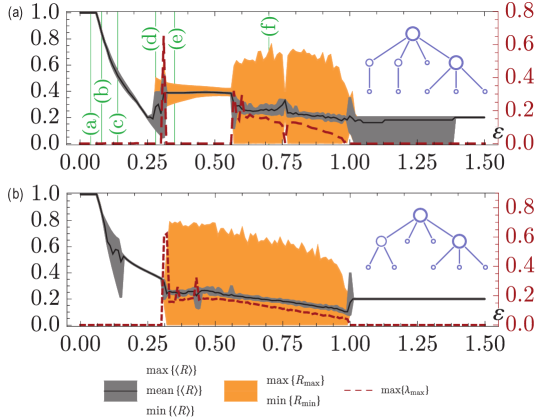
Figure 2: Numerical results for Model (1) as a function of $\varepsilon$, for the coupling graphs despited as insect, including 10 random initial conditions. A black line corresponds to $\mbox{mean}\!\left\{\!\hskip 1.13791pt\langle R\rangle\right\}$, while the interval between $\min\!\left\{\!\hskip 1.13791pt\langle R\rangle\right\}$ and $\max\!\left\{\!\hskip 1.13791pt\langle R\rangle\right\}$ is shown as a gray strip. The gap between $\min\!\left\{R_{\min}\right\}$ and $\max\!\left\{R_{\max}\right\}$ is shown as an orange strip. Since the orange strip is by construction larger or equal than the gray one, the first one is not displayed in the figure when they coincide. Left vertical axes show values related to norm of the order parameter, while the right ones represents the maximum Lyapunov exponent $\lambda_{\max}$, shown as a red dashed line. Letters in green vertical lines from the upper experiment correspond to subfigures in Fig. 3.

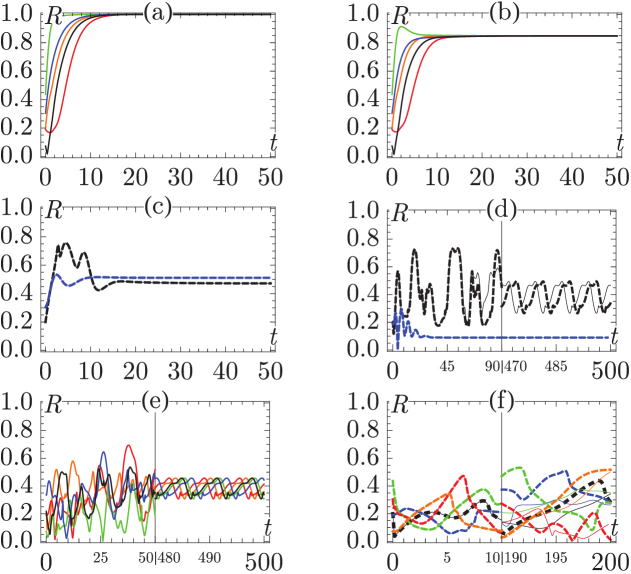
Figure 3: Evolution of $R\!\left(t\right)$ for different values of $\varepsilon$ indicated in green at the upper experiment from Fig. 2. Every color represents a different initial condition, while pairs of solid/dashed lines with the same color correspond to solutions whose initial conditions differ not more than $10^{-4}$ at each coordinate. (a) $\varepsilon=0.04$: full synchronization; (b) $\varepsilon=0.08$: fixed phase synchronization; (c,d,e) $\varepsilon=0.15,0.28,0.35$ respect.: examples of multi stability; (f) $\varepsilon=0.70$: example with $\lambda_{\max}>0$.

We now describe different regimes observed in the networks, using also Fig. 3, where we depict time series of $R\!\left(\theta\!\left(t\right)\right)$ for some particular choices of $\varepsilon$, indicated as green letters in the upper panel from Fig. 2 (this is the case we choose for illustrating different regimes). Notice that $d_{\max}=4$ in both cases, so Theorem 1 guarantees that for $\varepsilon<\varepsilon_{c}=1/4^{2}=0.0625$ the full synchronization state, $R\rightarrow 1$, is locally stable as illustrated in Fig. 3 (a) (with $\varepsilon=0.04$).

Panel (a) in Fig. 3 illustrates full synchronization in the network for $\varepsilon<\varepsilon_{c}$. For $\varepsilon$ slightly bigger than $\varepsilon_{c}$, simulations suggest that a stationary regime of partial phase synchronization, where $R\rightarrow c<1$, is locally stable as shown in Fig. 3(b) ($\varepsilon=0.08$). Details of this state are clear from Fig. 4. There we show the that the synchronization between the individual oscillators is complete if measured by quantity $s_{ij}$, and all the oscillators have the same frequency. However, the oscillators are split into two groups with a constant phase shift between them; this division originates in the edge which connects the two largest hubs in the network (vertexes $1,8$).

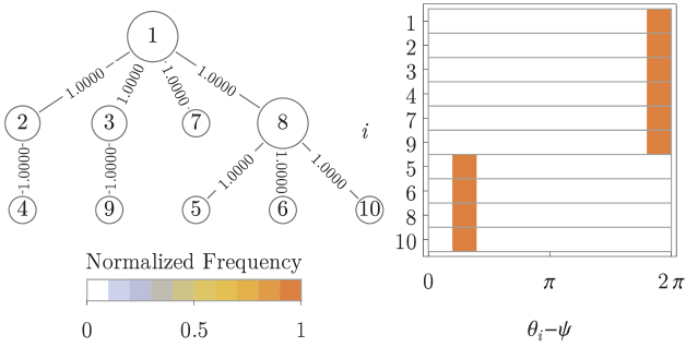
Figure 4: Example of group formation. Details of one of the trajectories from Fig. 3 (b) $\varepsilon=0.08$. On the left side, the coupling graph with $s\!\left(i,j\right)$ in its edges is shown. On the right side, a histogram of $\theta_{i}-\psi$ is presented with color code representing the normalized frequency.

For larger values of $\varepsilon$, the regimes are still static but with multistability. For instance, at $\varepsilon=0.15$ (see Fig. 3 (c)) two stable configurations emerge with $R\rightarrow c$, with $c\approx 0.471$ (black) or $c\approx 0.511$ (blue), depending on the initial condition. Fig. 5, which is analogous to Fig. 4, shows the existence of three subgroups, whose members may vary according to the initial condition.

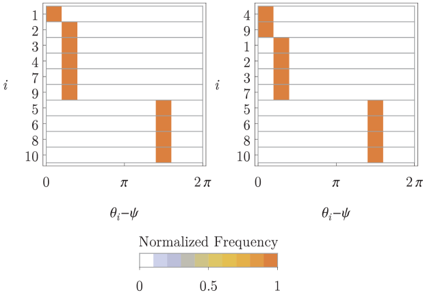
Figure 5: Example multi-stability with group formation. Details of two trajectories from Fig. 3 (c) $\varepsilon=0.15$, the left picture corresponds to the solid black line and the right one to the solid blue. Histograms of $\theta_{i}-\psi$ are presented with color code representing the normalized frequency.

Other types of multistabilities appear for instance at $\varepsilon=0.28$ and $\varepsilon=0.35$, as illustrate in Figs. 3 (d,e). For $\varepsilon=0.28$ (panel d) some initial conditions do no converge to a fixed phase synchronization, but to a regime where the order parameter $R$ is periodic in time. For $\varepsilon=0.35$ (panel c), the norm of the order parameter of all trajectories simulated becomes periodic. Fig. 6 provides an illustration of this regime.

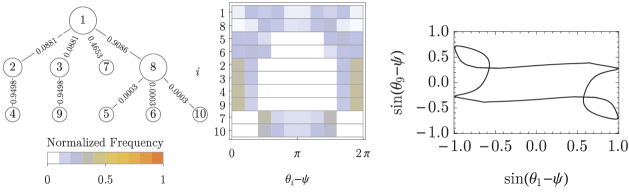
Figure 6: Example of periodic norm of the order parameter. Details of one of the trajectories from Fig. 3 (d) $\varepsilon=0.28$. On the left side, the coupling graph with $s\!\left(i,j\right)$ in its edges is shown. On the right side, a histogram of $\theta_{i}-\psi$ is presented with color code representing the normalized frequency. We denote by $\psi\!\left(t\right)$ the argument of the order parameter. The bottom picture shows that the curve $\!\left(\sin\!\left(\theta_{1}\!\left(t\right)-\psi\!\left(t\right)\right),\sin\!\left(\theta_{9}\!\left(t\right)-\psi\!\left(t\right)\right)\right)$ is closed.

Finally, for $\varepsilon=0.70$ (Fig. 3 (f)), one observes a chaotic state with $\lambda_{\max}>0$, the distribution of phases and frequencies is illustrated in Fig. 7.

If $\varepsilon\in\!\left[1,1.5\right]$, we also obtained multistability, with the coexistence of solutions converging to phase-lock and irregular order parameter after the transient, similar to Fig. 3(d).

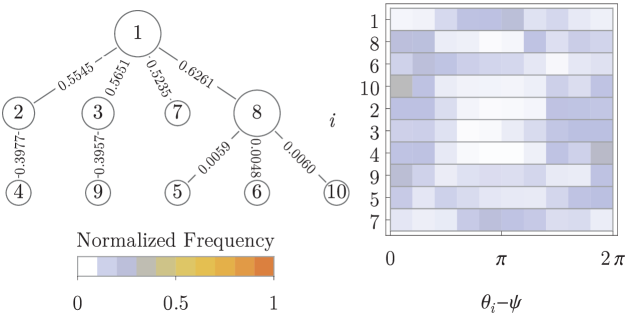
Figure 7: Example of trajectory with $\lambda_{\max}>0$. Details of one of the trajectories from Fig. 3 (f) $\varepsilon=0.70$. On the left side, the coupling graph with $s\!\left(i,j\right)$ in its edges is shown. On the right side, a histogram of $\theta_{i}-\psi$ is presented with color code representing the normalized frequency.

Now, we compare the results for two slightly different networks depicted in panels (a) and (b) in Fig. 2. The interval of values of $\varepsilon$ with fixed phase synchronization for all initial conditions simulated is very similar for both networks, namely $\varepsilon_{c}<\varepsilon\lesssim 0.25$; also multistability of static partial synchronous regimes have been observed in both cases.

When $\varepsilon\in\!\left[1,1.5\right]$, contrary to case (a), we observed that the solution for all initial conditions converged to the same phase-lock regime, similar to Fig. 3 (b).

In conclusion of this section, in Fig. 8 we show simulation results for two other networks. Panel (a) shows a random network with $N=10$ nodes and $20$ undirected edges. Here predominantly static regimes are observed, only in small ranges of coupling constant chaos with a positive Lyapunov exponent appears. Static regimes, however, demonstrate a large degree of multistability. In panel (b) we show a scale-free network with $N=50$ nodes and $100$ undirected edges. Here static states are rare, typically irregular regimes with low values of the order parameter are observed.

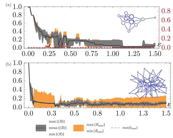
Figure 8: Numerical results for Model (1) as a function of $\varepsilon$, for the coupling graphs depicted as insect, including 10 random initial conditions. The legend of the pictures is the same as in Fig. 2

.

IV.3 Dependence of partial synchronization regimes on network structure

We have seen that partially synchronous states can be rather different even for similar networks. It is therefore difficult to make general predictions for a relation between the network properties and the dynamical behaviors. Here we attempt such a description, focusing on the property of abundance of static regimes in comparison to time-dependent ones. For this purpose we define the convergence index $I_{c}$ as the ratio of values of $\varepsilon\in\!\left[0,1.5\right]$ such that $R$ converges to a constant value, considering all the $10$ random initial conditions. So, both networks Fig. 2 have similar values of the index: $I_{c}\approx 0.530$ in case (a) while $I_{c}\approx 0.549$ in case (b). In contradistinction, network shown in Fig. 8(a) has very large value of the index $I_{c}\approx 0.946$, while that in Fig. 8(b) a rather low value $I_{c}\approx 0.064$.

In order to explore which features of the coupling graph are related with $I_{c}$, we performed numerical experiments with three sets of graphs, with $N=10,50,100$ nodes. Each set consists in three common types of networks, each one with $10$ members, generated as: (i) random (Erdös-Rényi) graphs with $2N$ edges; (ii) scale-free graphs, also with $2N$; and (iii) tree graphs ($N$ edges). The Barabási-Albert algorithm is applied for the last two types of networks (ii),(iii), with an initial clique of $m_{0}$ nodes and with other nodes been connected to $m$ existing ones. For the $2N$-edges scale-free graphs, we fixed $m_{0}=5$ and $m=2$; while for the tree graphs ($N$ edges scale-free graphs), $m_{0}=m=1$. We point out that all graphs created are connected and symmetrical. Additionally, three sets of $10$ initial conditions $\theta_{0}\in\mathbb{R}^{N}$, with uniform distribution over $\!\left[0,2\pi\right]$ and $N=10,50,100$, have been explored. So, for each of the $90$ coupling graphs we computed its correspondent $I_{c}$ values by numerical integration of model (1) for $\varepsilon=0,0.01,\ldots,1.49,1.50$.

In Table 1 we report the mean value and the standard deviation of $I_{c}$ for each topology and size of coupling graph. From these data we see that the mean value of $I_{c}$ increases if we go from tree to scale-free and to random graphs, respectively. However, these difference becomes less noticeable for larger values of $N$. Both the mean value and the standard deviation of $I_{c}$ decrease with larger networks.

Network	$N=10$	$N=50$	$N=100$
Tree	0.421 (0.260)	0.016 (0.006)	0.008 (0.004)
Scale-free	0.857 (0.029)	0.050 (0.015)	0.013 (0.003)
Random	0.872 (0.090)	0.183 (0.063)	0.077 (0.022)

Table 1: Mean value of $I_{c}$ and its standard deviation (in brackets) for each network type and size simulated.

We have explored different networks metrics, searching for one mostly correlated with the convergence index $I_{c}$. Let $0=\gamma_{1}<\gamma_{2}\leq\ldots\gamma_{N}$ denote the Laplacian eigenvalues of the coupling graph Godsil et al. (2001). Recall that this graph is assumed to be simple and connected. We stress that these eigenvalues express fundamental characteristics of the graph. For instance, $\gamma_{2}$ is related with graph diameter and $\gamma_{N}$ with its largest degree size.

We found that the quantity $\gamma^{*}$, defined as the ratio between the maximum eigenvalue and the average of the non-trivial eigenvalues of the Laplacian matrix of the graph, is rather suitable for this purpose. Formally, it is defined as

$$\gamma^{*}:=\gamma_{N}\!\left(\frac{1}{N-1}\sum\limits_{k=2}^{N-1}\gamma_{k}\right)^{-1}.$$

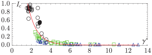
Figure 9: Convergence index $I_{c}$ versus $\gamma^{*}$. Networks with $N=10,50,100$ nodes are represented as circles, squares and triangles, respectively. The two experiments from Fig. 2 are shown as disks. We show in red an exponential fit $f\!\left(x\right)=\mathrm{e}^{1.7676-1.0894x}$ for the data.

In Fig. 9 a correlation plot between $I_{c}$ and measure $\gamma^{*}$ for the correspondent graph is presented. From there, we observe a clear trend indicating that the greater the value of $\gamma^{*}$ is, the smaller is the value of $I_{c}$. Independently of the network type and size, static regimes of partial synchronization, full synchronization and phase-lock, are typical for values of $\gamma^{*}\lesssim 3$, like in the experiments from Fig. 2. On the other hand, graphs with larger values of this measure yields more irregular dynamics, like time-dependent periodic and chaotic regimes, as the ones from Fig. 8.

V Conclusion

In this work we introduced and studied a Kuramoto-like model of identical oscillators with non-linear coupling. Our main parameter was $\varepsilon$, which governs the coupling nonlinearity strength. It is clear that the most influence of nonlinearity in the coupling is on the hubs which experience strong forcing from many connected oscillators, while less connected nodes may still operate in a linear-coupling regime.

We proved that if this parameter is smaller than the inverse of the square of the maximum vertex degree in the network, then the full synchronized state is stable. Via numerical experiments, we showed that our model can display a variety of other qualitative behaviors of partial synchronization, like stationary phase locking, multistability, periodic order parameter variations, and chaotic regimes. We explored the relative abundance of stationary phase locking regimes under different network topologies. Statistical analysis performed suggests that tree graphs are much less likely to exhibit stationary phase locking in comparison with scale-free or random networks. In addition, this type of behavior becomes more rare if we increase network sizes, irrespective to the network topology. Finally, we also found a good correlation between the ration between the maximum eigenvalue and the average of the non-trivial eigenvalues of the Laplacian matrix of the graph, and the proportion of the repulsion parameter values which yield stationary phase locking. The greater this measure is, the smaller tend to be presence of stationary phase locking states in the system.

As a future research, we want to investigate analytical conditions and correlations involving other graph measures related to other forms of synchronization in the model.