Self-Calibration and Biconvex Compressive Sensing
Abstract
The design of high-precision sensing devises becomes ever more difficult and expensive. At the same time, the need for precise calibration of these devices (ranging from tiny sensors to space telescopes) manifests itself as a major roadblock in many scientific and technological endeavors. To achieve optimal performance of advanced high-performance sensors one must carefully calibrate them, which is often difficult or even impossible to do in practice. In this work we bring together three seemingly unrelated concepts, namely Self-Calibration, Compressive Sensing, and Biconvex Optimization. The idea behind self-calibration is to equip a hardware device with a smart algorithm that can compensate automatically for the lack of calibration. We show how several self-calibration problems can be treated efficiently within the framework of biconvex compressive sensing via a new method called SparseLift. More specifically, we consider a linear system of equations , where both and the diagonal matrix (which models the calibration error) are unknown. By “lifting” this biconvex inverse problem we arrive at a convex optimization problem. By exploiting sparsity in the signal model, we derive explicit theoretical guarantees under which both and can be recovered exactly, robustly, and numerically efficiently via linear programming. Applications in array calibration and wireless communications are discussed and numerical simulations are presented, confirming and complementing our theoretical analysis.
1 Introduction
The design of high-precision sensing devises becomes ever more difficult and expensive. Meanwhile, the need for precise calibration of these devices (ranging from tiny sensors to space telescopes) manifests itself as a major roadblock in many scientific and technological endeavors. To achieve optimal performance of advanced high-performance sensors one must carefully calibrate them, which is often difficult or even impossible to do in practice. It is therefore necessary to build into the sensors and systems the capability of self-calibration – using the information collected by the system to simultaneously adjust the calibration parameters and perform the intended function of the system (image reconstruction, signal estimation, target detection, etc.). This is often a challenging problem requiring advanced mathematical solutions. Given the importance of this problem there has been a substantial amount of prior work in this area. Current self-calibration algorithms are based on joint estimation of the parameters of interest and the calibration parameters using standard techniques such as maximum likelihood estimation. These algorithms tend to be very computationally expensive and can therefore be used only in relatively simple situations. This has prevented their widespread applications in advanced sensors.
In this paper we take a step toward developing a new framework for self-calibration by bringing together three seemingly unrelated concepts, namely Self-Calibration, Compressive Sensing, and Biconvex Optimization. By “lifting” the problem and exploiting sparsity in the signal model and/or the calibration model we express the biconvex problem of self-calibration as a convex optimization problem, which can be solved efficiently via linear programming. This new method, called SparseLift, ensures equivalence between the biconvex problem and the convex problem at the price of a modest increase in the number of measurements compared to the already perfectly calibrated problem. SparseLift is inspired by PhaseLift, an algorithm for phase retrieval [12, 8], and by the blind deconvolution framework via convex programming due to Ahmed, Recht, and Romberg [1].
Self-calibration is a field of research in its own right, and we do not attempt in this paper to develop a framework that can deal with any kind of self-calibration problems. Instead our goal is more modest—we will consider a special, but at the same time in practice very important, class of self-calibration problems. To that end we first note that many self-calibration problems can be expressed as (either directly or after some modification such as appropriate discretization)
| (1.1) |
where represents the given measurements, is the system matrix depending on some unknown calibration parameters and is the signal (function, image, …) one aims to recover and is additive noise. As pointed out, we do not know exactly due to the lack of calibration. Our goal is to recover and from . More precisely, we want to solve
| (1.2) |
If depends linearly on , then (1.2) is a bilinear inverse problem. In any case, the optimization problem (1.2) is not convex, which makes its numerical solution rather challenging.
In many applications (1.1) represents an underdetermined system even if is perfectly known. Fortunately, we can often assume to be sparse (perhaps after expressing it in a suitable basis, such as a wavelet basis). Moreover, in some applications is also sparse or belongs to a low-dimensional subspace. Hence this suggests considering
| (1.3) |
where is a convex function that promotes sparsity in and/or . Often it is reasonable to assume that (1.3) is biconvex, i.e., it is convex in for fixed and convex in for fixed . In other cases, one can find a close convex relaxation to the problem. We can thus frequently interpret (1.3) as a biconvex compressive sensing problem.
Yet, useful as (1.3) may be, it is still too difficult and too general to develop a rigorous and efficient numerical framework for it. Instead we focus on the important special case
| (1.4) |
where is a diagonal matrix depending on the unknown parameters and is known. Of particular interest is the case where is sparse and the diagonal entries of belong to some known subspace. Hence, suppose we are given
| (1.5) |
where , , , , and is -sparse. can be interpreted as the unknown calibrating parameters lying in the range of a linear operator . Indeed, this model will be the main focus of our investigation in this paper. More examples and explanations of the model can be found in the next two subsections as well as in Sections 6.3 and 6.4.
Before moving on to applications, we pause for a moment to discuss the issue of identifiability. It is clear that if is a pair of solutions to (1.4), then so is ) for any non-zero . Therefore, it is only possible to uniquely reconstruct and up to a scalar. Fortunately for most applications this is not an issue, and we will henceforth ignore this scalar ambiguity when we talk about recovering and .
The reader may think that with the model in (1.4) we finally have reached a level of simplicity that is trivial to analyze mathematically and no longer useful in practice. However, as is often the case in mathematics, a seemingly simple model can be deceptive. On the one hand a rigorous analysis of the diagonal calibration model above requires quite non-trivial mathematical tools, and on the other hand this “simple” model does arise in numerous important applications. Perhaps the most widely known instance of (1.4) is blind deconvolution, see e.g. [1, 29]. Other applications include radar, wireless communications, geolocation, direction finding, X-ray crystallography, cryo-electron microscopy, astronomy, medical imaging, etc. We briefly discuss two such applications in more detail below.
1.1 Array self-calibration and direction-of-arrival estimation
Consider the problem of direction-of-arrival estimation using an array with antennas. Assuming that signals are impinging on the array, the output vector (using the standard narrowband model) is given by [37]
| (1.6) |
The (unknown) calibration of the sensors is captured by the matrix . By discretizing the array manifold , where are the azimuth and elevation angles, respectively, we can arrange equation (1.6) as (see [20])
| (1.7) |
where now also includes discretization error. Here is a completely known function of and does not depend on calibration parameters, so is a known matrix.
To give a concrete example, assuming for simplicity all sensors and signal sources lie in the same plane, for a circular array with uniformly spaced antennas, the -th column of the matrix is given by with where is a discretization of the angular domain (the possible directions of arrival), the entries of represent the geometry of the sensor array, is the number of sensors, and is the array element spacing in wavelengths.
An important special case is when is a diagonal matrix whose diagonal elements represent unknown complex gains associated with each of the antennas. The calibrating issue may come from position offsets of each antenna and/or from gain discrepancies caused by changes in the temperature and humidity of the environment. If the true signal directions lie on the discretized grid of angles corresponding to the columns of , then the vector is -sparse, otherwise is only approximately -sparse. In the direction finding problem we usually have multiple snapshots of the measurements , in which case and in (1.7) become matrices, whose columns are associated with different snapshots [20].
1.2 The Internet of Things, random access, and sporadic traffic
The Internet of Things (IoT) will connect billions of wireless devices, which is far more than the current Fourth-Generation (4G) wireless system can technically and economically accommodate. One of the many challenges of 5G, the future and yet-to-be-designed wireless communication system, will be its ability to manage the massive number of sporadic traffic generating IoT devices which are most of the time inactive, but regularly access the network for minor updates with no human interaction [40]. Sporadic traffic will dramatically increase in the 5G market and it is a common understanding among communications engineers that this traffic cannot be handled within the current 4G random access procedures. Dimensioning the channel access according to classical information and communication theory results in a severe waste of resources which does not scale towards the requirements of the IoT. This means among others that the overhead caused by the exchange of certain types of information between transmitter and receiver, such as channel estimation, assignment of data slots, etc, has to be avoided. In a nutshell, if there is a huge number of devices each with the purpose to sporadically transmit a few bits of data, we must avoid transmitting each time a signal where the part carrying the overhead information is much longer than the part carrying the actual data. The question is whether this is possible.
In mathematical terms we are dealing with the following problem (somewhat simplified, but it captures the essence). For the purpose of exposition we consider the single user/single antenna case. Let denote the channel impulse response and the signal to be transmitted, where is a sparse signal, its non-zero coefficients containing the few data that need to be transmitted. We encode by computing , where is a fixed precoding matrix, known to the transmitter and the receiver. However, the non-zero locations of are not known to the receiver, and nor is , since this is the overhead information that we want to avoid transmitting, as it will change from transmission to transmission. The received signal is given by the convolution of and , i.e., . The important point here is that the receiver needs to recover from , but does not know either. This type of problem is often referred to as blind deconvolution. After applying the Fourier transform on both sides and writing (where denotes the Fourier transform), we obtain , which is of the form (1.4) modulo a change of notation. A more detailed example with concrete choices for and is given in Section 6.4.
1.3 Notation and outline
Matrices are written in uppercase boldface letters (e.g. ), while vectors are written in lowercase boldface letters (e.g. ), and scalars are written in regular font or denoted by Greek letters. For a matrix with entries we denote , is the nuclear norm of , i.e., the sum of its singular values; , is the operator norm of and is its Frobenius norm. denotes the trace of . If is a vector, is its 2-norm and denotes the number of non-zero entries in , and denotes the complex conjugate of
The remainder of the paper is organized as follows. In Section 2 we briefly discuss our contributions in relation to the state of the art in self-calibration. Section 3 contains the derivation of our approach and the main theorems of this paper. Sections 4 and 5 are dedicated to the proofs of the main theorems. We present numerical simulations in Section 6 and conclude in Section 7 with some open problems.
2 Related work and our contributions
Convex optimization combined with sparsity has become a powerful tool; it provides solutions to many problems which were believed intractable in the fields of science, engineering and technology. Two remarkable examples are compressive sensing and matrix completion. Compressive sensing [18, 13, 19], an ingenious way to efficiently sample sparse signals, has made great contributions to signal processing and imaging science. Meanwhile, the study of how to recover a low-rank matrix from a seemingly incomplete set of linear observations has attracted a lot of attention, see e.g. [5, 7, 33].
Besides drawing from general ideas in compressive sensing and matrix completion, the research presented in this work is mostly influenced by papers related to PhaseLift [4, 12, 30] and in particular by the very inspiring paper on blind deconvolution by Ahmed, Recht, and Romberg [1]. PhaseLift provides a strategy of how to reconstruct a signal from its quadratic measurements via “lifting” techniques. Here the key idea is to lift a vector-valued quadratic problem to a matrix-valued linear problem. Specifically, we need to find a rank-one positive semi-definite matrix which satisfies linear measurement equations of : where Generally problems of this form are NP-hard. However, solving the following nuclear norm minimization yields exact recovery of
| (2.1) |
This idea of ”Lifting” also applies to blind deconvolution [1], which refers to the recovery of two unknown signals from their convolution. The model can be converted into the form (3.1) via applying the Fourier transform and under proper assumptions can be recovered exactly by solving a nuclear norm minimization program in the following form,
| (2.2) |
if the number of measurements is at least larger than the dimensions of both and . Compared with PhaseLift (2.1), the difference is that can be asymmetric and there is of course no guarantee for positivity. Ahmed, Recht, and Romberg derived a very appealing framework for blind deconvolution via convex programming, and we borrow many of their ideas for our proofs.
The idea of our work is motivated by the two examples mentioned above and our results are related to and inspired by those of Ahmed, Recht, and Romberg. However, there are important differences in our setting. First, we consider the case where one of the signals is sparse. It seems unnecessary to use as many measurements as the signal length and solve (2.2) in that case. Indeed, as our results show we can take much fewer measurements in such a situation. This means we end up with a system of equations that is underdetermined even in the perfectly calibrated case (unlike [1]), which forces us to exploit sparsity to make the problem solvable. Thus [1] deals with a bilinear optimization problem, while we end up with a biconvex optimization problem. Second, the matrix in [1] is restricted to be a Gaussian random matrix, whereas in our case can be a random Fourier matrix as well. This additional flexibility is relevant in real applications. For instance a practical realization of the application in 5G wireless communications as discussed in Section 1.2 and Section 6.4 would never involve a Gaussian random matrix as spreading/coding matrix, but it could definitely incorporate a random Fourier matrix.
Bilinear compressive sensing problems have also been investigated in e.g. [16, 38, 28]. These papers focus on the issue of injectivity and the principle of identifiability. Except for the general setup, there is little overlap with our work. Self-calibration algorithms have been around in the literature for quite some time, see e.g. [21, 35, 2, 31] for a small selection, with blind deconvolution being a prominent special case, cf. [29] and the references therein. It is also worth noting that [24, 3, 34] have developed self-calibration algorithms by using sparsity, convex optimization, and/or ideas from compressive sensing. In particular, [24, 3] give many motivating examples of self-calibration and propose similar methods by using the lifting trick and minimizing or to exploit sparsity and/or low-rank property. While these algorithms are definitely useful and interesting and give many numerical results, most of them do not provide any guarantees of recovery. To the best of our knowledge, our paper is the first work to provide theoretical guarantee for recovery after bringing self-calibration problems into the framework of biconvex compressive sensing. Uncertainties in the sensing matrix have been analyzed for instance in [26, 15], but with the focus on quantifying the uncertainty, while our current work can be seen as a means to mitigate the uncertainty in the sensing matrix.
3 Self-calibration, biconvex optimization, and SparseLift
As discussed in the introduction, we are concerned with , where the diagonal matrix and are unknown. Clearly, without further information it is impossible to recover (or ) from since the number of unknowns is larger than the number of measurements. What comes to our rescue is the fact that in many applications additional knowledge about and is available. Of particular interest is the case where is sparse and the diagonal entries of belong to some known subspace.
Hence, suppose we are given
| (3.1) |
where , , , , and is -sparse. E.g., may be a matrix consisting of the first columns of the DFT (Discrete Fourier Transform) matrix which represents a scenario where the diagonal entries in are slowly varying from entry to entry. One may easily formulate the following optimization problem to recover and ,
| (3.2) |
We can even consider adding an -component in order to promote sparsity in ,
| (3.3) |
However, both programs above are nonconvex. For (3.2), it is an optimization with a bilinear objective function because it is linear with respect to one vector when the other is fixed. For (3.3), the objective function is not even bilinear but biconvex [22].
3.1 SparseLift
To combat the difficulties arising from the bilinearity of the objective function in (3.2), we apply a novel idea by “lifting” the problem to its feasible set [8, 12] . It leads to a problem of recovering a rank-one matrix instead of finding two unknown vectors. Denote by the -th column of and by the -th column of . A little linear algebra yields
| (3.4) |
Let and define the linear operator ,
Now the problem is to find a rank-one matrix satisfying the linear constraint where is the true matrix. A popular method is to take advantage of the rank-one property and use nuclear norm minimization.
where denotes the nuclear norm of which is the sum of singular values.
Before we proceed, we need a bit of preparations. By using the inner product defined on as , the adjoint operator of and have their forms as
We also need a matrix representation of such that
| (3.5) |
reshapes matrix into a long column vector in lexicographic order. For each , follows from the property of Kronecker product, where is the complex conjugate of . It naturally leads to the block form of ,
| (3.6) |
With all those notations in place, the following formula holds
also has an explicit representation of its columns. Denote
| (3.7) |
and are the -th and -th column of and respectively. Both and are of the size . Then we can write into
Assume we pick a subset with , we define from and also has its matrix representation as
| (3.8) |
such that and
Concerning the support of , and , we can assume without loss of generality that the support of is its first entries and thus have its first columns nonzero. By a slight abuse of notation, we write for the supports of , and . Let and denote the orthogonal projections of and on , respectively. Define and as the restriction of and onto ,
| (3.9) |
One can naturally define with non-zero columns satisfying and with non-zero columns such that
Even if we stipulate that the degrees of freedom in is smaller than by assuming that the diagonal entries of belong to some subspace, without any further knowledge about the self-calibration problem is not solvable, since the number of unknowns exceeds the number of measurements. Fortunately, in many cases we can assume that is sparse. Therefore, the matrix is not only of rank one but also sparse. A common method to recover from is to use a linear combination of and as an objective function (See [30] for an example in phase retrieval) and solve the following convex program
| (3.10) |
(3.10) tries to impose both sparsity and rank-one property of a matrix. While (3.10) seems a natural way to proceed, we will choose a somewhat different optimization problem for two reasons. First, it may not be straightforward to find a proper value for , see also Figures 2 and 3 in Section 6. Second, in [32] it is shown that if we perform convex optimization by combining the two norms as in (3.10), then we can do no better, order-wise, than an algorithm that exploits only one of the two structures. Since only minimizing requires (which can be too large for large ) and there also holds for any matrix , both of them suggest that perhaps in certain cases it may suffice to simply try to minimize , which in turn may already yield a solution with sparse structure and small nuclear norm. Indeed, as well will demonstrate, -minimization performs well enough to recover exactly under certain conditions although it seemingly fails to take advantage of the rank-one property. Hence we consider
| (3.11) |
This idea first lifts the recovery problem of two unknown vectors to a matrix-valued problem and then exploits sparsity through -minimization. We will refer to this method as SparseLift. It takes advantage of the “linearization” via lifting, while maintaining the efficiency of compressive sensing and linear programming.
If the observed data are noisy, i.e., with , we take the following alternative convex program
| (3.12) |
3.2 Main results
Our main finding is that SparseLift enables self-calibration if we are willing to take a few more additional measurements. Furthermore, SparseLift is robust in presence of additive noise. In our theory we consider two choices for the matrix : in the one case is a Gaussian random matrix; in the other case consists of rows chosen uniformly at random with replacement from the Discrete Fourier Transform (DFT) matrix with . In the latter case, we simply refer to as a random Fourier matrix. Note that we normalize to simply because where is a column of .
Theorem 3.1.
Consider the model (3.1) and assume that is an tall matrix with , is a dense vector and is an -sparse and vector. Then the solution to is equal to with probability at least if
-
1.
is an real Gaussian random matrix with with each entry and
(3.15) -
2.
is an random Fourier matrix with and
(3.16) where .
In both cases is growing linearly with and is defined as the largest absolute value in the matrix , i.e.,
Remarks: We note that , and . The definition of seems strict but it contains a lot of useful and common examples. For example, a matrix has if each column is picked from an unitary DFT matrix and We expect the magnitude of each entry in does not vary too much from entry to entry and thus the rows of are incoherent.
Theorem 3.2.
If the observed is contaminated by noise, namely, with , the solution given by (3.12) has the following error bound.
-
1.
If is a Gaussian random matrix,
with probability of success at least . satisfies and both and are both constants.
-
2.
If is a random Fourier matrix,
with probability of success at least . and satisfy and both and are both constants
The proof of the theorem above is introduced in Section 5. The solution obtained by SparseLift, see (3.11) or (3.12) for noisy data, is not necessarily rank-one. Therefore, we compute the singular value decomposition of and set and , where is the leading singular value and and are the leading left and right singular vectors, respectively.
Corollary 3.3.
Let be the best Frobenius norm approximation to , then there exists a scalar and a constant such that
where
[1, 12, 9] also derived error bounds of recovering the signals from the recovered ”lifted” matrix by using the leading eigenvector or leading left and right singular vectors. [12, 9] focus on PhaseLift and the recovered vector from is unique up to a unit-normed scalar. Our corollary is more similar to Corollary 1 in [1] because both of them deal with a bilinear system instead of a quadratic system like PhaseLift. There are two signals to recover from in our case and thus they are unique up to a scalar . Without prior information, no theoretical estimate can be given on how large is.
4 Proof of Theorem 3.1
The outline of the proof of Theorem 3.1 follows a meanwhile well-established pattern in the literature of compressive sensing [14, 19] and low-rank matrix recovery, but as is so often the case, the difficulty lies in the technical details. We first derive sufficient conditions for exact recovery. The fulfillment of these conditions involves computing norms of certain random matrices as well as the construction of a dual certificate. The main part of the proof is dedicated to these two steps. While the overall path of the proof is similar for the case when is a Gaussian random matrix or a random Fourier matrix, there are several individual steps that are quite different.
4.1 A sufficient condition for exact recovery
We will first give a sufficient condition for exact recovery by using SparseLift. Then we prove all the proposed assumptions are valid.
Proposition 4.1.
This proposition can be regarded as a sufficient condition of exact recovery of a sparse vector via minimization in compressive sensing (See Theorem 4.26(a) in [19]. They are actually the same but appear in different formulations). Based on (4.1), we propose an alternative sufficient condition which is much easier to use.
Proposition 4.2.
is the unique minimizer if there exists a satisfying the following conditions,
| (4.2) |
and the linear operator satisfies
| (4.3) |
Proof: .
The proof starts with . Note that if and . By splitting the inner product of on and , the following expression can guarantee the exact recovery of minimization,
By using the Hölder inequality, we arrive at the stronger condition
| (4.4) |
Due to and , we have and . As a result,
| (4.5) |
The second equality follows from . Substitute (4.5) into (4.4) and we only need to prove the following expression in order to achieve exact recovery,
If and , the above expression is strictly positive. On the other hand, implies from (4.5). Therefore, the solution of SparseLift equals if the proposed conditions (4.3) and (4.2) are satisfied.
4.2 Local isometry property
In this section, we will prove Lemma 4.3, the local isometry property, which achieves the first condition in (4.3).
Lemma 4.3.
In fact, it suffices to prove Lemma 4.6 and Lemma 4.7 because Lemma 4.3 is a special case of Lemma 4.7 when and .
4.2.1 Two ingredients of the proof
Before we move to the proof of Lemma 4.6 and Lemma 4.7, we introduce two important ingredients which will be used later. One ingredient concerns the rows of . There exists a disjoint partition of index set into with each and such that
| (4.6) |
The existence of such a partition follows from the proof of Theorem 1.2 in [11] and is used in Section 3.2 of [1]. (4.6) also can give a simple bound for the operator norms of both and
| (4.7) |
The other ingredient concerns the non-commutative Bernstein inequality. For Gaussian and Fourier cases, the inequalities are slightly different. This following theorem, mostly due to Theorem 6.1 in [36], is used for proving the Fourier case of (4.20).
Theorem 4.4.
Consider a finite sequence of of independent centered random matrices with dimension . Assume that and introduce the random matrix
| (4.8) |
Compute the variance parameter
| (4.9) |
then for all
For the Gaussian case we replace with where the norm of a matrix is defined as
The concentration inequality is different if is Gaussian because of the unboundedness of . We are using the form in [27].
4.2.2 A key lemma and its proof
For each subset of indices , we denote
| (4.11) |
Under certain conditions, it is proven that does not deviate from the identity much for each . We write this result into Lemma 4.6.
Lemma 4.6.
For any equal partition of with such that (4.6) holds true (e.g. let ), we have
| (4.12) |
with probability at least if
-
1.
is the -th row of an Gaussian random matrix and .
-
2.
is the -th row of an random Fourier matrix and .
In both cases grows linearly with respect to and .
First, we prove the following key lemma. Lemma 4.6 is a direct result from Lemma 4.7 and the property stated in (4.6). We postpone the proof of Lemma 4.6 to Section 4.2.3.
Lemma 4.7.
Proof: .
We prove the Gaussian case first; the proof of the Fourier case is similar. Let be a standard Gaussian random vector. denotes the projected vector on the support of with . We first rewrite the linear operator into matrix form. Using the Kronecker product we define as follows:
| (4.14) |
Every is a centered random matrix since , which follows from restricting to the support and taking its expectation. is an matrix with as its leading submatrix. It is easy to check that
More precisely, in needs to be replaced by according to the property of Kronecker product. But there is no problem here since each is a real random vector. For simplicity, we denote . In order to use Theorem 4.5 to estimate , we need to know and . We first give an estimate for the operator norm of .
| (4.15) |
Here is a random variable with degrees of freedom. This implies that , following from Lemma 6 in [1]. Therefore there exists an absolute constant such that
The second step is to estimate . It suffices to consider because is a Hermitian matrix.
The expectation of is
| (4.16) |
following from which can be proven by using similar reasoning of Lemma 9 in [1].
| (4.17) | |||||
| (4.18) | |||||
| (4.19) |
where the inequality in the second line follows from and the positivity of . The only thing to do is to estimate before we can apply the concentration inequality (4.10). We claim that there holds
for some constant . Notice that and is at most of order . It suffices to show the lower bound of in order to prove the expression above. Following from (4.17), we have On the other hand, (4.6) leads to since the trace of a positive semi-definite matrix must be greater than its operator norm. Therefore we conclude that because and
Now we are well prepared to use (4.10). can be simply treated as a matrix for each because its support is only With , and we have
Now we let where is a function which grows linearly with respect to and has sufficiently large derivative. By properly assuming , is also greater than and
We take the union bound over all and have
This completes the proof for the Gaussian case.
We proceed to the Fourier case. The proof is very similar and the key is to use Theorem 4.4. Now we assume is the -th row of a random Fourier matrix and thus . Here because is a complex random vector. However, it does not change the proof at all except the notation. Like the proof of the Gaussian case, we need to know and also . Following the same calculations that yielded (4.15), (4.16) and (4.19), we have
and
Then we apply Theorem 4.4 and obtain
if we pick . This implies
4.2.3 Proof of Lemma 4.6
4.2.4 Estimating the operator norm of
The operator norm of with will be given for both the Gaussian case and the Fourier case such that for any with high probability. For the Gaussian case, Lemma 1 in [1] gives the answer directly.
Lemma 4.8.
For the Fourier case, a direct proof will be given by using the non-commutative Bernstein inequality in Theorem 4.4.
Lemma 4.9.
For defined in (3.4) with a random Fourier matrix and fixed ,
| (4.22) |
with probability at least if we choose
Proof: .
First note that . Therefore it suffices to estimate the norm of
The second equality follows from the fact that . For each centered random matrix we have and
That means . In order to estimate the variance of each , we only have to compute since is a Hermitian matrix.
Hence the variance of is
Now we apply Bernstein’s inequality and for any , we have
Suppose , then
If we pick , then
If , we have
with probability at least .
4.3 Construction of the dual certificate
In the last section we have shown that (4.3) holds true. Now we will prove that a satisfying (4.2) exists by explicitly constructing it for both, the Gaussian and the Fourier case.
4.3.1 is a Gaussian random matrix
Construction of Exact dual certificate via least square method:
It follows from Lemma 4.3 and 4.6 that is invertible on with
if for some scalar . We construct the exact dual
certificate via (see [6])
| (4.23) |
Let ; it suffices to consider and verify whether and .
Theorem 4.10.
Conditioned on the event , there holds
with probability at least if we pick .
Proof: .
Note and is independent of for because only uses In this case,
where is an standard Gaussian random vector. Due to the independence between and ,
where
Therefore, is a centered Gaussian random variable with variance at most . For any , we have
Taking the union bound over all pairs of indices satisfying gives
If we pick , then and
Choosing implies that the probability of will be less than
4.3.2 is a random Fourier matrix
Construction of Inexact dual certificate via golfing scheme:
An inexact dual certificate will be constructed to satisfy the conditions given in (4.2) via the
golfing scheme, which was first proposed in [25] and has been widely
used since then, see e.g. [1, 19, 30]. The idea is to use part of the measurements in each step and construct
a sequence of random matrices recursively in . The sequence converges to
exponentially fast and at the same time keeps each entry of small on . We initialize and set
| (4.24) |
We denote . Let be the residual between and on and . yields the following relations due to (4.24),
where is defined in (4.11). Following from Lemma 4.6, decreases exponentially fast with respect to with probability at least and
| (4.25) |
The value of can be determined to make . Hence,
| (4.26) |
The next step is to bound the infinity norm of on . We first rewrite the recursive relation (4.24); has the following form,
| (4.27) |
Our aim is to achieve . It suffices to make in order to make is the operator which orthogonally projects a matrix onto . For each ,
since is known at step and is independent of . has the same support as does and thus this gives The next theorem proves that for all with probability at least if and
Theorem 4.11.
Conditioned on (4.25) and for fixed ,
In particular this gives
by choosing and taking the union bound for all .
Proof: .
For any where has support , we have
directly following from (3.4) and (3.5). Therefore,
where is a unit vector with its -th entry equal to . Here because only the first entries of are nonzero. The main idea of the proof is to estimate for each and take the union bound over all For any fixed
Let . Notice because
and have the same support and thus any entry of on equals to . Therefore each is a bounded and centered random variable. We can use scalar version of Bernstein inequality (a special version of Theorem 4.4) to estimate First we estimate
There holds , which follows from the fact that is a row of DFT matrix and each entry of is of unit magnitude. Moreover, has support ,
Therefore, The variance of is estimated as
and
Now we apply the Bernstein inequality in Theorem 4.4 and have the estimate for
Note that is independent of and hence the inequality above is still valid if we choose . Since and , we have
We take the union bound over all and obtain
5 Proof of Theorem 3.2
Now we consider the noisy case by solving the convex program (3.14). Our goal is to prove Theorem 3.2. The main ingredient of our proof is Theorem 4.33 in [19]. A variant of that theorem, adapted to our setting, reads as follows.
Theorem 5.1.
Let be the columns of , with support on and with . For and ,
| (5.1) |
and that there exists a vector with such that
| (5.2) |
If , then the minimizer to (3.14) satisfies
| (5.3) |
where and are two scalars only depending on and
Actually, we have already proven in the previous section that we can choose . The only two unknown components are and . follows from computing the norm of We need to know the coherence of to estimate and claim that . Define the coherence as the largest correlation between two different columns of the matrix ,
| (5.4) |
where is defined in (3.7).
5.1 Estimation of and .
It is easy to obtain a bound of for and with ,
It suffices to bound by in order to achieve . The following lemma (see Lemma A.9 in [19]) will be used in the proof.
Lemma 5.2.
For any matrix , any entry is bounded by its operator norm, i.e.,
| (5.5) |
Theorem 5.3.
There holds
with probability at least if
-
1.
is a Gaussian random matrix and and .
-
2.
is a random Fourier matrix and and .
Here, in both cases is a function growing at most linearly with respect to .
Proof: .
We only prove the Gaussian case by using Lemma 4.3. The proof of the Fourier case is exactly the same. First we pick any two different columns and from , where and . Let be
| (5.6) |
and contains and . By Lemma 4.3, with probability if . Therefore follows from Lemma 5.2. Then we take the union bound over pairs of indices and . Therefore, with and probability at least if .
5.2 Proof of Theorem 3.2 when is a Gaussian random matrix
5.3 Proof of Theorem 3.2 when is a random Fourier matrix
Proof: .
We have an explicit form of from (4.27)
such that , and is an inexact dual certificate. The norm of is
For each ,
which follows from (4.25) and in Lemma 4.6. Therefore,
This implies where is chosen in (4.26). We also have , and which are the same as Gaussian case and Now we have everything needed to apply Theorem 5.1. The solution to (3.14) satisfies
with , and , are two constants.
6 Numerical simulations
6.1 Recovery performance of SparseLift
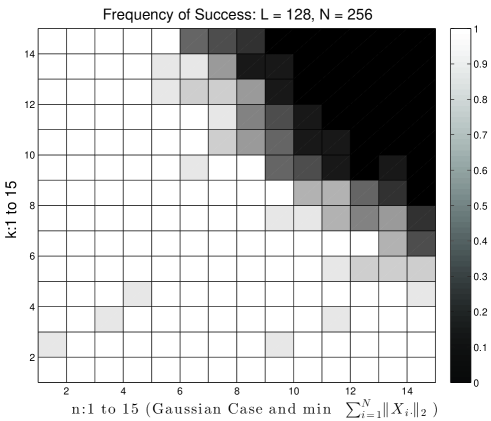
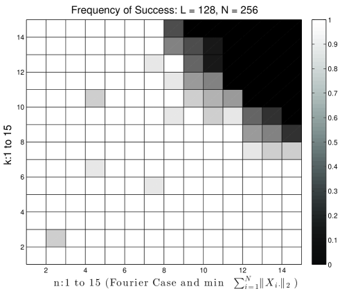
We investigate the empirical probability of success of SparseLift over different pairs of for fixed and . We fix , and make both and range from to . We choose as the first columns of an unitary DFT matrix and is sampled independently for each experiment. has random supports with cardinality and the nonzero entries of and yield . For each , we run 10 times and compute the probability of success. We classify a recovery as a success if the relative error is less than ,
Note that SparseLift is implemented by using CVX package [23]. The results are depicted in Figure 1. The phase transition plots are similar for the case when is a Gaussian random matrix or a random Fourier matrix. In this example choosing gives satisfactory recovery performance via solving SparseLift.

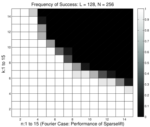
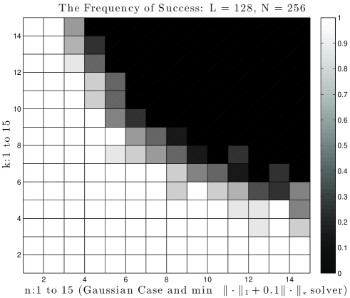
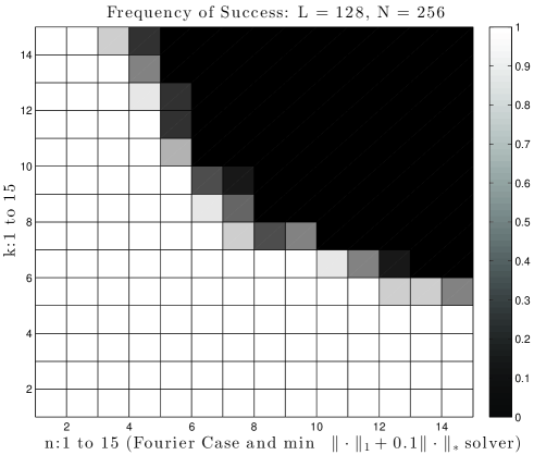
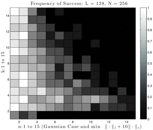
For comparison, we illustrate the performance when we solve the convex optimization problem that combines the nuclear norm and sparsity as in (3.10), see Figures 2 and 3. The values for are (the best value for for this experiment) and . The settings of other parameters are exactly the same as the scenario of solving SparseLift. Figure 2 shows that (3.10) with performs similar to solving . However, if the results are clearly worse in general, in particular for the Gaussian case, see Figure 3. For Fourier case, choosing might do better than SparseLift for some pairs of . The reason behind this phenomenon is unclear yet and may be due to solver we choose and numerical imprecision. All the numerical results support our hypothesis that the performance of recovery is sensitive to the choice of and SparseLift is good enough to recover calibration parameters and the signal in most cases with theoretic guarantee. This is in line with the findings in [32] which imply that convex optimization with respect to a combination of the norms and will not perform significantly better than using only one norm, the -norm in this case.
We also show the performance when using a mixed --norm to enforce column-sparsity in instead of just -norm. In this case we note a slight improvement over (3.11). As mentioned earlier, analogous versions of our main results, Theorem 3.1 and Theorem 3.2, hold for the mixed --norm case as well and will be reported in a forthcoming paper.

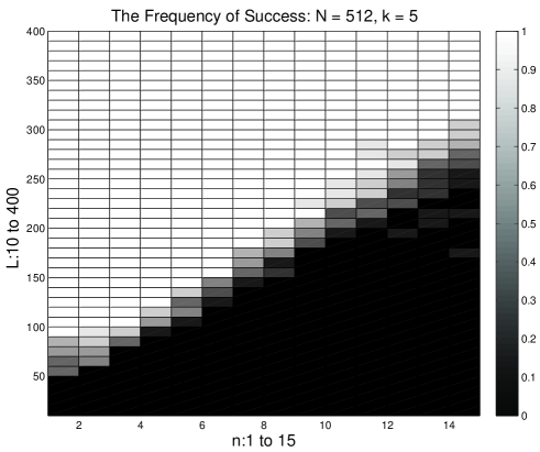
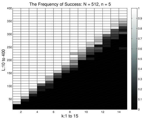
6.2 Minimal required for exact recovery is proportional to
The minimal which guarantees exact recovery is nearly proportional to , as shown in Figure 5. The figure shows the results of two experiments: one is to keep and let vary from 1 to 15; the other is to fixe and let range from 1 to 15. In both experiments, is chosen to be , varies from 10 to 400 and is chosen to be a Gaussian random matrix. We run 10 simulations for each set of and treat a recovery as a success if the relative error is less than The result provides numerical evidence for the theoretical guarantee that SparseLift yields exact recovery if .
We also notice that the ratio of minimal against is slightly larger in the case when is fixed and varies than in the other case. This difference can be explained by the -term because the larger is, the larger is needed.
However, these numerical observations do not imply that the minimum required by a different (numerically feasible) algorithm also has to be proportional to . Indeed, it would be very desirable to have an efficient algorithm with provable recovery guarantees for which on the order of about (modulo some log-factors) measurements suffice.
6.3 Self-calibration and direction-of-arrival estimation
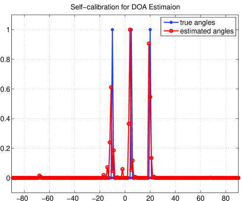
We examine the array self-calibration problem discussed in Section 1.1. We consider a scenario of three fully correlated equal-power signals. Note that the case of fully correlated signals is much harder than the case of uncorrelated (or weakly correlated) signals. Standard methods like MUSIC [39] will in general fail completely for fully correlated signals even in the absence of any calibration error. The reason is that these methods rely on the additional information obtained by taking multiple snapshots. Yet, for fully correlated signals all snapshots are essentially identical (neglecting noise) and therefore no new information is contained in multiple snapshots.
We use a circular array consisting of omni-directional sensors. We assume that the calibration error is changing slowly across sensors, as for example in the case of sensors affected by changing temperature or humidity. There are of course many possibilities to model such a smooth change in calibration across sensors. In this simulation we assume that the variation can be modeled by a low-degree trigonometric polynomial (the periodicity inherent in trigonometric polynomials is fitting in this case, due to the geometry of the sensors); in this example we have chosen a polynomial of degree 3. To be precise, the calibration error, i.e., the complex gain vector is given by , where is a matrix, whose columns are the first four columns of the DFT matrix and is a vector of length 4, whose entries are determined by taking a sample of a multivariate complex Gaussian random variable with zero mean and unit covariance matrix. The stepsize for the discretization of the grid of angles for the matrix is 1 degree, hence (since we consider angles between and ). The directions of arrival are set to , and , and the SNR is 25dB. Since the signals are fully correlated we take only one snapshot.
We apply SparseLift, cf. (3.14), to recover the angles of arrival. Since the sensing matrix does not fulfill the conditions required by Theorem 3.2 and the measurements are noisy, we cannot expect SparseLift to return a rank-one matrix. We therefore extract the vector with the angles of arrival by computing the right singular vector associated with the largest singular value of . As can be seen in Figure 6 the estimate obtained via self-calibration provides a quite accurate approximation to the true solution.
6.4 5G, the Internet of Things, and SparseLift
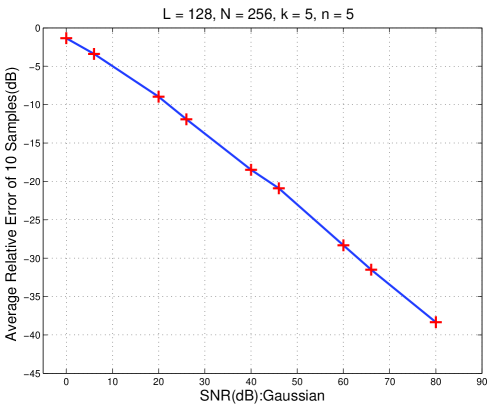
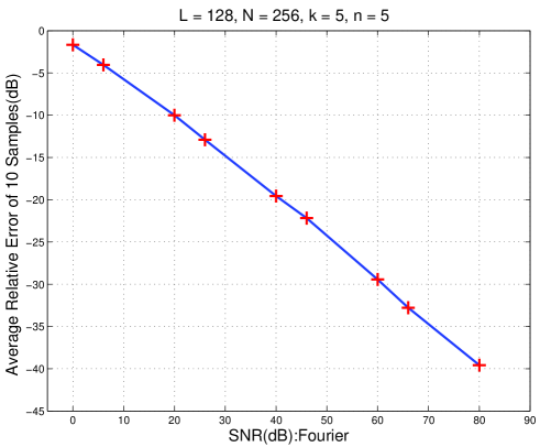
We briefly discussed in Section 1.2 how self-calibration problems of the form analyzed in this paper are anticipated to play a role in 5G wireless communication systems in connection with the Internet of Things, sporadic traffic and random access. Let us assume we deal with a CDMA communication scheme. To accommodate as many sporadic users as possible, we consider an “overloaded” CDMA system. This means that the matrix containing the so-called spreading sequences (aptly called spreading matrix) has many more columns than rows. We use a random Fourier matrix for that purpose. Furthermore, we assume that the transmission channel is frequency-selective and time-invariant for the time of transmission of one sequence, but it may change from transmission to transmission. The channel is unknown at the receiver, it only knows an upper bound on the delay spread (the length of the interval containing the non-zero entries of ). Moreover, the transmitted signal experiences additive Gaussian noise. The mathematician who is not familiar with all this communications jargon may rest assured that this is a standard scenario in wireless communication. In essence it translates to a linear system of equations of the form , where is a flat random Fourier matrix, is of the form and is AWGN. To be specific, we choose the transmitted signal to be of length with data-bearing coefficients (thus, ), the locations of which are chosen at random. The 256 spreading sequences of length are generated by randomly selecting 128 rows from the DFT matrix. Thus the system is overloaded by a factor of 2. The delay spread is assumed to be 5, i.e., and the matrix consists of the first 5 columns of the unitary DFT matrix. The SNR ranges from 0dB to 80dB (the latter SNR level is admittedly unrealistic in practical scenarios).
We attempt to recover by solving (3.12). Here we assume and We choose as [1] in order to make inside the feasible set.
The result is depicted in Figure 7; for comparison we also show the results when using a Gaussian random matrix as spreading matrix. We plot the relative error (on a dB scale) for different levels of (also on a dB scale). The horizontal axis represents and the vertical axis represents . We run 10 independent experiments for each SNR level and take the average relative error. The error curves show clearly the desirable linear behavior between SNR and mean square error with respect to the log-log scale.
7 Conclusion and outlook
Self-calibration is an emerging concept that will get increasingly important as hardware and software will become more and more intertwined. Several instances of self-calibration, such as blind deconvolution, have already been around for some time. In this work we have taken a step toward building a systematic mathematical framework for self-calibration. There remain more open questions than answers at this stage. Some obvious extensions of the results in this paper will be to consider the case where both and are sparse. Another useful generalization is the scenario where is replaced by a matrix, like in the direction-of-arrival problem with multiple snapshots. Lifting the self-calibration problem in this case would lead to a tensor-valued (instead of a matrix-valued) underdetermined linear system [20]. The computational complexity for solving the associated relaxed convex problem will likely be too expensive for practical purposes and other methods will be needed. Extensions of the Wirtinger-Flow approach in [10] seem to be a promising avenue to derive computationally efficient algorithms for this and other self-calibration scenarios. Another important generalization is the case when there is mutual coupling between sensors, in which case is no longer a diagonal matrix. Yet another very relevant setting consists of depending non-linearly on , as is often the case when the sensors are displaced relative to their assumed locations. In conclusion, we hope that it has become evident that self-calibration is on the one hand an inevitable development in sensor design in order to overcome some serious current limitations, and on the other hand it is a rich source of challenging mathematical problems.
Acknowledgement
T.S. wants to thank Benjamin Friedlander from UC Santa Cruz for introducing him to the topic of self-calibration. The authors acknowledge generous support from the NSF via grant DTRA-DMS 1042939.
References
- [1] A. Ahmed, B. Recht, and J. Romberg. Blind deconvolution using convex programming. Information Theory, IEEE Transactions on, 60(3):1711–1732, 2014.
- [2] L. Balzano and R. Nowak. Blind calibration of sensor networks. In Proceedings of the 6th international conference on Information processing in sensor networks, pages 79–88. ACM, 2007.
- [3] C. Bilen, G. Puy, R. Gribonval, and L. Daudet. Convex optimization approaches for blind sensor calibration using sparsity. Signal Processing, IEEE Transactions on, 62(18):4847–4856, 2014.
- [4] E. Candès, Y. Eldar, T. Strohmer, and V. Voroninski. Phase retrieval via matrix completion. SIAM J. Imag. Sci., 6(1):199–225, 2013.
- [5] E. Candès and B. Recht. Exact matrix completion via convex optimization. Foundations of Computational Mathematics, 9(6):717–772, 2009.
- [6] E. Candès and B. Recht. Simple bounds for low-complexity model reconstruction. Technical report, 2011.
- [7] E. Candès and T. Tao. The Power of Convex Relaxation: Near-Optimal Matrix Completion. IEEE Trans. Inform. Theory, 56(5):2053–2080, 2010.
- [8] E. J. Candès, Y. C. Eldar, T. Strohmer, and V. Voroninski. Phase retrieval via matrix completion. SIAM Journal on Imaging Sciences, 6(1):199–225, 2013.
- [9] E. J. Candes and X. Li. Solving quadratic equations via phaselift when there are about as many equations as unknowns. Foundations of Computational Mathematics, pages 1–10, 2012.
- [10] E. J. Candes, X. Li, and M. Soltanolkotabi. Phase retrieval via wirtinger flow: Theory and algorithms. Information Theory, IEEE Transactions on, 61(4):1985–2007, 2015.
- [11] E. J. Candès and J. Romberg. Sparsity and incoherence in compressive sampling. Inverse problems, 23(3):969, 2007.
- [12] E. J. Candès, T. Strohmer, and V. Voroninski. Phaselift: Exact and stable signal recovery from magnitude measurements via convex programming. Communications on Pure and Applied Mathematics, 66(8):1241–1274, 2013.
- [13] E. J. Candès and T. Tao. Near-optimal signal recovery from random projections: Universal encoding strategies. IEEE Trans. on Information Theory, 52:5406–5425, 2006.
- [14] E. Cands and Y. Plan. A Probabilistic and RIPless Theory of Compressed Sensing. IEEE Transactions on Information Theory, 57(11):7235–7254, 2011.
- [15] Y. Chi, L. L. Scharf, A. Pezeshki, and A. R. Calderbank. Sensitivity to basis mismatch in compressed sensing. Signal Processing, IEEE Transactions on, 59(5):2182–2195, 2011.
- [16] S. Choudhary and U. Mitra. Identifiability scaling laws in bilinear inverse problems. arXiv preprint arXiv:1402.2637, 2014.
- [17] C. Davis and W. M. Kahan. The rotation of eigenvectors by a perturbation. iii. SIAM Journal on Numerical Analysis, 7(1):1–46, 1970.
- [18] D. L. Donoho. Compressed sensing. IEEE Trans. on Information Theory, 52(4):1289–1306, 2006.
- [19] S. Foucart and H. Rauhut. A mathematical introduction to compressive sensing. Springer, 2013.
- [20] B. Friedlander and T. Strohmer. Bilinear compressed sensing for array self-calibration. In Asilomar Conference Signals, Systems, Computers, Asilomar, 2014.
- [21] B. Friedlander and A. J. Weiss. Self-calibration for high-resolution array processing. In S. Haykin, editor, Advances in Spectrum Analysis and Array Processing, Vol. II, chapter 10, pages 349–413. Prentice-Hall, 1991.
- [22] J. Gorski, F. Pfeuffer, and K. Klamroth. Biconvex sets and optimization with biconvex functions: a survey and extensions. Mathematical Methods of Operations Research, 66(3):373–407, 2007.
- [23] M. Grant, S. Boyd, and Y. Ye. Cvx: Matlab software for disciplined convex programming, 2008.
- [24] R. Gribonval, G. Chardon, and L. Daudet. Blind calibration for compressed sensing by convex optimization. In Acoustics, Speech and Signal Processing (ICASSP), 2012 IEEE International Conference on, pages 2713–2716. IEEE, 2012.
- [25] D. Gross. Recovering low-rank matrices from few coefficients in any basis. Information Theory, IEEE Transactions on, 57(3):1548–1566, 2011.
- [26] M. A. Herman and T. Strohmer. General deviants: An analysis of perturbations in compressed sensing. Selected Topics in Signal Processing, IEEE Journal of, 4(2):342–349, 2010.
- [27] V. Koltchinskii et al. Von Neumann entropy penalization and low-rank matrix estimation. The Annals of Statistics, 39(6):2936–2973, 2011.
- [28] K. Lee, Y. Wu, and Y. Bresler. Near optimal compressed sensing of sparse rank-one matrices via sparse power factorization. Preprint, arXiv:1312.0525, 2013.
- [29] A. Levin, Y. Weiss, F. Durand, and W. Freeman. Understanding blind deconvolution algorithms. Pattern Analysis and Machine Intelligence, IEEE Transactions on, 33(12):2354–2367, 2011.
- [30] X. Li and V. Voroninski. Sparse signal recovery from quadratic measurements via convex programming. SIAM Journal on Mathematical Analysis, 45(5):3019–3033, 2013.
- [31] A. Liu, G. Liao, C. Zeng, Z. Yang, and Q. Xu. An eigenstructure method for estimating DOA and sensor gain-phase errors. IEEE Trans. Signal Processing, 59(12):5944–5956, 2011.
- [32] S. Oymak, A. Jalali, M. Fazel, Y. C. Eldar, and B. Hassibi. Simultaneously structured models with application to sparse and low-rank matrices. Information Theory, IEEE Transactions on, 61(5):2886–2908, 2015.
- [33] B. Recht, M. Fazel, and P. Parrilo. Guaranteed minimum rank solutions of matrix equations via nuclear norm minimization. SIAM Review, 52(3):471–501, 2010.
- [34] C. Schulke, F. Caltagirone, F. Krzakala, and L. Zdeborova. Blind calibration in compressed sensing using message passing algorithms. Advances in Neural Information Processing Systems, 26:566–574, 2013.
- [35] C. See. Sensor array calibration in the presence of mutual coupling and unknown sensor gains and phases. Electronics Letters, 30(5):373–374, 1994.
- [36] J. A. Tropp. User-friendly tail bounds for sums of random matrices. Foundations of Computational Mathematics, 12(4):389–434, 2012.
- [37] T. Tuncer and B. Friedlander, editors. Classical and Modern Direction-of-Arrival Estimation. Academic Press, Boston, 2009.
- [38] P. Walk and P. Jung. A stability result for sparse convolutions. Preprint, arXiv.org/abs/1312.2222, 2013.
- [39] A. Weiss and B. Friedlander. Eigenstructure methods for direction finding with sensor gain and phase uncertainties. J. Circuits, Systems and Signal Processing, 9(3):271–300, 1989.
- [40] G. Wunder, H. Boche, T. Strohmer, and P. Jung. Sparse signal processing concepts for efficient 5g system design. IEEE Access, accepted, 2014. Preprint available at arXiv.org/abs/1411.0435.
- [41] Y. Zhang, J. Yang, and W. Yin. Yall1: Your algorithms for l1. MATLAB software, http://www. caam. rice. edu/~ optimization L, 1, 2010.