Estimation of parameters of SDE driven by fractional Brownian motion with polynomial drift

Abstract

Strongly consistent and asymptotically normal estimators of the Hurst index and volatility parameters of solutions of stochastic differential equations with polynomial drift are proposed. The estimators are based on discrete observations of the underlying processes.

Keywords: fractional Brownian motion, Hurst index, volatility, Black-Scholes model, Verhulst equation, Landau-Ginzburg equation, consistent estimator

¹ Vilnius University, Institute of Mathematics and Informatics, Akademijos 4,

LT-08663 Vilnius, Lithuania

² Vilnius University, Faculty of Mathematics and Informatics, Naugarduko 24,

LT-03225, Vilnius, Lithuania

³ Vilnius Gediminas Technical University, Saulėtekio al. 11,

LT-10223, Vilnius, Lithuania

1 Introduction

Many applications use processes that are described by stochastic differential equations (SDE). Recently, much attention has been paid to SDEs driven by the fractional Brownian motion (fBm) and to the problems of statistical estimation of model parameters. Statistical aspects of the models including fBm were studied in many articles. Especially much attention was paid to the estimations of the parameter of drift. We concentrate on estimation of the Hurst parameter and volatility of SDE with polynomial drift

$$X_{t}=\xi+\int_{0}^{t}\big{(}aX_{s}^{m}+bX_{s}\big{)}ds+c\int_{0}^{t}X_{s}\,dB^{H}_{s},\quad\xi\geqslant 0,\quad t\in[0,T],$$ (1)

where $1/2<H<1$, $m\in\mathbb{N}$, $m\geqslant 2$, and $B^{H}$ is a fBm with Hurst index $1/2<H<1$. Almost all sample paths of $B^{H}$ have bounded $p$-variation for each $p>1/H$ on $[0,T]$ for every $T>0$ (a more detailed definition of an fBm will be formulated in the next section). The second integral in (1) is the pathwise Riemann-Stieltjes integral with respect to the process having finite $p$-variation.

It is well known that equation (1) for standard Brownian motion, i. e. for $H=1/2$, is nonlinear reducible SDE with polynomial drift of degree $m$. Under the substitution $h(x)=x^{1-m}$ equation (1) reduces to a linear SDE with multiplicative noise. Some famous equations can be obtained as particular cases of this equation. For example, we can obtain the Black-Scholes model, the Verhulst and the Landau-Ginzburg equations.

Using an approximation approach in $L^{2}$ Dung [7] obtained an explicit solution of the equation (1) for $H>1/2$. His approximation is based on the fact that fBm of Liouville form can be uniformly approximated by semimartingales.

Many authors (see [8], [9], [3], [5], [1], [2], [16], [14], [13]) considered an almost sure convergence and an asymptotic normality of the generalized quadratic variations associated to the filter $a$ (see [9]) of a wide class of processes with Gaussian increments. Conditions for this type of convergence are expressed in terms of covariances of a Gaussian process and depend on some parameter $\gamma\in(0,2)$. These results make it possible to obtain an estimator of the parameter $\gamma$ and to study its asymptotic properties. If the process under consideration is the fBm then this parameter is the Hurst index $0<H<1$.

There are a few results concerning estimation of the Hurst index if the observed process is described by SDE driven by fBm. For the first time, to our knowledge, an estimator of the Hurst parameter of a pathwise solution of a linear SDE driven by a fBm and its asymptotical behaviour were considered in [4]. A more general situation was considered in [10] using a different approach. Estimators for the Hurst parameter were constructed making use of the first and second order quadratic variations of the observed values of the solution. Only the strong consistency of these estimators was proved. A comparison of different estimators of the Hurst index for linear SDE driven by fBm was carried out in [11]. A rate of convergence of these estimators with probability $1$ to the true value of a parameter was obtained in [12], when the maximum length of the interval partition tends to zero.

In this paper we will use a different approach to solving the equation (1) than suggested by N. T. Dung. We apply a pathwise approach to stochastic integral equations and use a chain rule for the composition of a smooth function and a function of bounded $p$-variation with $1<p<2$. This approach allows us to simplify the proof of existence and uniqueness of the solution of the equation (1). The goal of the paper is to construct strongly consistent and asymptotically normal estimators of the Hurst parameter and the volatility of SDE (1) using discrete observations of the sample paths of the solution of the SDE. Estimators are constructed using quadratic variations of second order increments. Estimators’ properties are determined asymptotically from the properties of quadratic variations.

The paper is organized in the following way. In Section 2 we present the main results of the paper. Section 3 is devoted to several known results needed for the proofs. In Section 4 we prove the uniqueness of SDE (1) and give its explicit solution. Sections 5.1–5.3 contain the proofs of the main results. Finally, in Section 6 some simulations are given in order to illustrate the obtained results.

2 Main results

Let $X$ be a stochastic process satisfying (1). Denote

$$\Delta^{(2)}_{n,k}X=X_{n,k+1}-2X_{n,k}+X_{n,k-1},\qquad\Delta_{n,k+1}X=X_{n,k+1}-X_{n,k},$$

where $X_{n,k}=X(t^{n}_{k})$, $t^{n}_{k}=\frac{kT}{n}$. For the sake of simplicity, we shall omit the index $n$ for points $t_{k}^{n}$ and for notions $X_{n,k}$, $\Delta^{(2)}_{n,k}$, $\Delta_{n,k}$, where the sample size is equal to $n$. In case of different sample sizes the indices will be retained.

In the formulation of Theorem 2 as well as in the sequel we make use of the symbols $O_{r},o_{r}$. Here is a brief explanation. Let $(a_{n})$ be a sequence of real numbers. $Y_{n}=O_{r}(a_{n})$, $a_{n}\downarrow 0$, means that there exists a.s. finite r.v. $\varsigma$ with the property $|Y_{n}|\leqslant\varsigma\cdot a_{n}$; $Y_{n}=o_{r}(a_{n})$ means that $|Y_{n}|\leqslant\varsigma\cdot b_{n}$ with $b_{n}=o(a_{n})$. Particulary $Y_{n}=o_{r}(1)$ denotes the sequence $(Y_{n})$ which tends to $0$ a.s. as $n\to\infty$.

Theorem 1

Assume that $X$ is a solution of SDE (1) with $a\leqslant 0$. Let $X_{0}>0$, $c\neq 0$, and $1/2<H<1$. Then

$$\widehat{H}^{(1)}_{n} \longrightarrow H\quad\mbox{a.s.,}$$

$$2\sqrt{n}\,\ln\frac{n}{T}\,(\widehat{H}^{(1)}_{n}-H) \xrightarrow{\ d\ }\mathcal{N}(0,\sigma^{2})$$ (2)

with a known variance $\sigma^{2}=\sigma^{2}(H)$ defined in Subsection 3.2, where for $n>T$

$$\widehat{H}^{(1)}_{n}= \varphi_{n,T}^{-1}\Bigg{(}\frac{1}{n}\sum_{k=1}^{n-1}\left(\frac{\Delta^{(2)}_{k}X}{cX_{k}}\right)^{2}\Bigg{)},$$

$$\varphi_{n,T}(x)= \Big{(}\frac{T}{n}\Big{)}^{2x}(4-2^{2x})\quad\text{ and }\quad\varphi_{n,T}^{-1}\ \mbox{is the inverse function of}\ \varphi_{n,T},\quad x\in(0,1).$$

Theorem 1 gives an estimator of $H$ under the assumption that $c$ is known. This is not always the case. Therefore we present another estimator which is suitable when $c$ is unknown.

Theorem 2

Let assumptions of Theorem 1 hold and

$$\widehat{H}^{(2)}_{n}=\frac{1}{2}-\frac{1}{2\ln 2}\ln\left(\frac{\sum_{k=1}^{2n-1}\left(\frac{\Delta^{(2)}_{2n,k}X}{X_{2n,k}}\right)^{2}}{\sum_{k=1}^{n-1}\left(\frac{\Delta^{(2)}_{n,k}X}{X_{n,k}}\right)^{2}}\right).$$

Then

$$\widehat{H}^{(2)}_{n} \longrightarrow H\quad\mbox{a.s.,}$$

$$2\ln 2\,\sqrt{n}(\widehat{H}^{(2)}_{n}-H) \xrightarrow{\ d\ }\mathcal{N}(0,\sigma_{*}^{2})$$ (3)

with a known variance $\sigma_{*}^{2}=\sigma_{*}^{2}(H)$ defined in Subsection 3.2.

To estimate $c$ one can use the last theorem provided below.

Theorem 3

Assume that $1/2<H<1$ and $\widehat{H}^{(3)}_{n}=H+o_{r}(\phi(n))$ a.s. If $\phi(n)=o\left(\frac{1}{\ln n}\right)$ then

$$\widehat{c}^{\,2}_{n}= \frac{n^{2\widehat{H}^{(3)}_{n}-1}}{T^{2\widehat{H}^{(3)}_{n}}(4-2^{2\widehat{H}^{(3)}_{n}})}\sum_{k=1}^{n-1}\left(\frac{\Delta^{(2)}_{k}X}{X_{k}}\right)^{2}\longrightarrow c^{2}\quad\mbox{a.s.;}$$

if $\phi(n)=o\left(\frac{1}{\sqrt{n}\ln n}\right)$ then $\sqrt{n}\,(\widehat{c}^{\,2}_{n}-c^{2})\xrightarrow{\ d\ }\mathcal{N}(0,c^{4}\sigma^{2})$.

Hence estimation of $c$ and construction of confidence intervals is always possible. However confidence intervals will shrink at the rate which is a bit worse than the usual $n^{-1/2}$.

3 Preliminaries

3.1 Variation

In this subsection we remind several facts about $p$–variation. For details we refer the reader to [6]. Recall that a function $f:[a,b]\to\mathbb{R}$ has $p$–variation defined by

$$v_{p}(f;[a,b])=\sup_{\varkappa}\sum_{k=1}^{n}\lvert f(x_{k})-f(x_{k-1})\rvert^{p},$$

where $p\in(0,\infty)$ is a fixed number and supremum is taken over all possible partitions

$$\varkappa:a=x_{0}<x_{1}<\dots<x_{n}=b,\qquad n\geqslant 1.$$

If $v_{p}(f;[a,b])<\infty,$ $f$ is said to have a bounded $p$-variation on $[a,b].$ Denote by $\mathcal{W}_{p}([a,b])$ the class of functions defined on the $[a,b]$ with bounded $p$–variation. Let $C\mathcal{W}_{p}([a,b])$ denote the class of functions that have bounded $p$–variation and are continuous. Define $V_{p}(f;[a,b])=v_{p}^{1/p}(f;[a,b])$, which is a seminorm on $\mathcal{W}_{p}([a,b])$ provided $p\geqslant 1$ and $V_{p}(f;[a,b])$ is $0$ if and only if $f$ is a constant.

If $f\in\mathcal{W}_{p}([a,b])$, then f is bounded and $f\in\mathcal{W}_{p_{1}}([a,b])$ for every $p_{1}>p\geqslant 1$. Let $0<p<\infty$ and $f,g\in\mathcal{W}_{p}([a,b])$. Then $fg\in\mathcal{W}_{p}([a,b])$.

Let $f\in\mathcal{W}_{q}([a,b])$ and $h\in\mathcal{W}_{p}([a,b])$ with $0<p<\infty$, $q>0,$ $1/p+\allowbreak 1/q>1.$ Then the integral $\int_{a}^{b}f\,\mathrm{d}h$ exists as the Riemann–Stieltjes integral if $f$ and $h$ have no common discontinuities. If the integral exists, the Love–Young inequality

$$\Bigg{|}\int\limits_{a}^{b}f\,\hbox{\rm d}h-f(y)\big{[}h(b)-h(a)\big{]}\Bigg{|}\leqslant C_{p,q}V_{q}\big{(}f;[a,b]\big{)}V_{p}\big{(}h;[a,b]\big{)}$$ (4)

holds for all $y\in[a,b]$, where $C_{p,q}=\zeta(p^{-1}+q^{-1})$ and $\zeta(s)=\sum_{n\geqslant 1}n^{-s}.$

Let $f\in{\mathcal{W}}_{q}([a,b])$ and $h\in{\mathcal{W}}_{p}([a,b]).$ From (4) it follows that

$$V_{p}\Bigg{(}\int\limits_{a}^{\hbox{$\bf\cdot$}}f\,\hbox{\rm d}h;[a,b]\Bigg{)}\leq C_{p,q}V_{q,\infty}\big{(}f;[a,b]\big{)}V_{p}\big{(}h;[a,b]\big{)},$$

where $V_{q,\infty}(f;[a,b])=V_{q}(f;[a,b])+\sup_{a\leqslant x\leqslant b}|f(x)|$. Note that $V_{q,\infty}(f;[a,b])$ is a norm on ${\mathcal{W}}_{q}([a,b])$, $q\geqslant 1$.

If $h\in C{\mathcal{W}}_{p}([a,b])$, then the indefinite integral $\int_{a}^{y}f\,\hbox{\rm d}h$, $y\in[a,b]$, is a continuous function.

To verify that some process solves the equation (1) we use a chain rule for the composition of a smooth function and a function of bounded $p$-variation with $0<p<2$. The chain rule is based on the Riemann–Stieltjes integrals. As usual, the composition $g\circ h$ on $[a,b]$ of two functions $g$ and $h$ is defined by $(g\circ h)(x)=g(h(x))$ whenever $h$ is defined on $[a,b]$ and $g$ on the range of $h$.

Theorem 4 (Chain rule (see [6]))

Let $f=(f_{1},\ldots,f_{d}):[a,b]\to\mathbb{R}^{d}$ be a function such that, for each $k=1,\ldots,d$, $f_{k}\in C\mathcal{W}_{p}([a,b])$ with $1\leqslant p<2$. Let $g:\mathbb{R}^{d}\to\mathbb{R}$ be a differentiable function with locally Lipschitz partial derivatives $g^{\prime}_{k}$, $k=1,\ldots,d$. Then each $g^{\prime}_{l}\circ f$ is Riemann-Stieltjes integrable with respect to $f_{k}$ and

$$(g\circ f)(b)-(g\circ f)(a)=\sum_{k=1}^{d}\int_{a}^{b}(g_{k}^{\prime}\circ f)\,df_{k}.$$

Proposition 5 (Substitution rule (see [6]))

Let $f$, $g$, and $h$ be functions in $C\mathcal{W}_{p}([a,b])$, $1\leqslant p<2$. Then

$$\int_{a}^{b}f(x)\,d\bigg{(}\int_{a}^{x}g(y)\,dh(y)\bigg{)}=\int_{a}^{b}f(x)g(x)\,dh(x).$$

3.2 Several results on fBm

Recall that fBm $B^{H}=\{B^{H}_{t}\colon\ t\geqslant 0\}$ with Hurst index $H\in(0,1)$ is a real-valued continuous centered Gaussian process with covariance given by

$$\hbox{\bf E}(B^{H}_{t}B^{H}_{s})=\frac{1}{2}\big{(}s^{2H}+t^{2H}-|t-s|^{2H}\big{)}.$$

For consideration of strong consistency and asymptotic normality of the given estimators we need several facts about $B^{H}$.

Limit results. Let

$$V_{n,T}=\frac{n^{2H-1}}{4-2^{2H}}\sum_{k=1}^{n-1}\big{(}T^{-H}\Delta^{(2)}_{n,k}B^{H}\big{)}^{2},\qquad H\neq\frac{1}{2}\,.$$

Then (see [3], [9], [2])

$$V_{n,T}\xrightarrow[n\to\infty]{}1\quad\text{ a.s.;}$$

$$\sqrt{n}\left(\begin{array}[]{c}V_{n,T}-1\\ V_{2n,T}-1\\ \end{array}\right)\xrightarrow{\ d\ }\mathcal{N}\left(\left(\begin{array}[]{c}0\\ 0\\ \end{array}\right),\left(\begin{array}[]{cc}\sigma^{2}(H)&\sigma_{1,2}(H)\\ \sigma_{1,2}(H)&\sigma^{2}(H)/2\\ \end{array}\right)\right)$$

with

$$\sigma^{2}(H)=2+c_{2}(H)+c_{1}(H)\sum_{l=2}^{\infty}\big{(}\rho_{2-2H}(l)\big{)}^{2},\qquad\sigma_{1,2}(H)=2^{-2H}\big{(}3\sigma^{2}+\sigma_{1}^{2}+4\sigma_{2}^{2}\big{)},$$

where

$$c_{1}(H)= \left(\frac{2H(2H-1)(2H-2)(2H-3)}{4-2^{2H}}\right)^{2},\,\quad c_{2}(H)=\left(\frac{2^{2H+2}-7-3^{2H}}{4-2^{2H}}\right)^{2},$$

$$\rho_{2-2H}(l)= \frac{\lvert l-2\rvert^{2H}-4\lvert l-1\rvert^{2H}+6\lvert l\rvert^{2H}-4\lvert l+1\rvert^{2H}+\lvert l+2\rvert^{2H}}{2H(1-2H)(2-2H)(3-2H)}\,,\quad l\in\mathbb{Z},$$

$$\sigma_{1}^{2}= \frac{c_{2}(H)}{2}+c_{1}(H)\sum_{l=2}^{\infty}\rho_{2-2H}(l)\,\rho_{2-2H}(l-2),$$

$$\sigma_{2}^{2}= 2\sqrt{c_{2}(H)}+c_{1}(H)\sum_{l=2}^{\infty}\rho_{2-2H}(l)\,\rho_{2-2H}(l-1).$$

These relationships imply that

$$\widetilde{H}_{n}=\frac{1}{2}-\frac{1}{2\ln 2}\ln\left(\frac{V_{2n,T}}{2^{2H-1}V_{n,T}}\right)\to H\text{ a.s.,}$$

$$2\ln 2\,\sqrt{n}(\widetilde{H}_{n}-H)\xrightarrow{\ d\ }\mathcal{N}(0;\sigma_{*}^{2}(H)),\qquad\sigma_{*}^{2}(H)=\frac{3}{2}\sigma^{2}(H)-2\sigma_{1,2}(H).$$

Variation of $B^{H}$. It is known that almost all sample paths of an fBm $B^{H}$ are locally Hölder of order strictly less than $H$, $0<H<1$. To be more precise, for all $0<\varepsilon<H$ and $T>0$, there exists a nonnegative random variable $G_{\varepsilon,T}$ such that $\mathbb{E}(|G_{\varepsilon,T}|^{p})<\infty$ for all $p\geqslant 1$, and

$$|B^{H}_{t}-B^{H}_{s}|\leqslant G_{\varepsilon,T}|t-s|^{H-\varepsilon}\qquad a.s.$$ (5)

for all $s,t\in[0,T]$. Thus $B^{H}\in C\mathcal{W}_{H_{\varepsilon}}([0,T])$, ${H_{\varepsilon}}=\frac{1}{H-\varepsilon}$.

SDE driven by fBm $B^{H}$. A solution of the stochastic integral equation (1), on a given filtered probability space $(\Omega,\,{\mathcal{F}},\,{\bf P},\,\mathbb{F})$ and with respect to the fixed fBm $(B^{H},\,\mathbb{F}),$ $1/2<H<1,$ and initial condition $\xi$, is an adapted to the filtration $\mathbb{F}$ continuous process $X=\{X_{t}\colon\ 0\leq t\leq T\}$ such that $X_{0}=\xi$ a.s., ${\bf P}(\int_{0}^{t}|f(X_{s})|\,ds+\big{|}\int_{0}^{t}g(X_{s})\,dB^{H}_{s}\big{|}<\infty)=1$ for every $0\leq t\leq T,$ and its almost all sample paths satisfy (1).

4 Solution of SDE with polynomial drift

First, we consider a non-random integral equation

$$x_{t}=x_{0}+\int_{0}^{t}(ax_{s}^{m}+bx_{s})\,ds+c\int_{0}^{t}x_{s}\,dh_{s},\qquad x_{0}\geqslant 0,\quad a\leqslant 0,\ t\in[0,T],$$ (6)

where $m\in\mathbb{N}$, $m\geqslant 2$, $h\in C\mathcal{W}_{p}([0,T])$, $1<p<2$.

4.1 Uniqueness of the solution of equation (6)

Theorem 6

The integral equation (6) has a unique solution in the class of functions $C\mathcal{W}_{p}([0,T])$, $1<p<2$.

Proof. It is well-known that

$$a^{m}-b^{m}=(a-b)\sum_{k=0}^{m-1}a^{k}b^{m-1-k}.$$

Let us assume that we have two solutions $x_{t}$ and $y_{t}$ of equation (6). Since the solutions belong to the class of functions $C\mathcal{W}_{p}([0,T])$, $1<p<2$, then

$$|x_{t}^{m}-y_{t}^{m}|\leqslant mL_{x,y,m,T}|x_{t}-y_{t}|,$$

where

$$L_{x,y,m,T}=\Big{(}\max\Big{\{}\max_{0\leqslant t\leqslant T}|x_{t}|,\max_{0\leqslant t\leqslant T}|y_{t}|\Big{\}}\Big{)}^{m-1}.$$

Further, one can find a subdivision $\tau=\{0<\tau_{1}<\tau_{2}<\cdots<\tau_{n}=T\}$ such that

$$V_{p}(h;[\tau_{k-1},\tau_{k}])\leqslant\big{(}4|c|C_{p,p}\big{)}^{-1}$$

for all $k$. Assume we have proved that $x_{\tau_{k-1}}=y_{\tau_{k-1}}$. Then

$$V_{p,\infty}(x-y;[\tau_{k-1},\tau_{k}])= V_{p,\infty}(x-y-(x_{\tau_{k-1}}-y_{\tau_{k-1}});[\tau_{k-1},\tau_{k}])$$

$$\leqslant 2|a|\int_{\tau_{k-1}}^{\tau_{k}}|x^{m}_{t}-y^{m}_{t}|\,dt+2|b|\int_{\tau_{k-1}}^{\tau_{k}}|x_{t}-y_{t}|\,dt$$

$$+2|c|C_{p,p}V_{p,\infty}(x-y;[\tau_{k-1},\tau_{k}])V_{p}(h;[\tau_{k-1},\tau_{k}])$$

$$\leqslant \big{(}2L_{x,y,m,T}|a|+2|b|\big{)}\int_{\tau_{k-1}}^{\tau_{k}}|x_{t}-y_{t}|\,dt$$

$$+2|c|C_{p,p}V_{p,\infty}(x-y;[\tau_{k-1},\tau_{k}])V_{p}(h;[\tau_{k-1},\tau_{k}])$$

and

$$V_{p,\infty}(x-y;[\tau_{k-1},\tau_{k}])\leqslant 4\big{(}L_{x,y,m,T}|a|+|b|\big{)}\int_{\tau_{k-1}}^{\tau_{k}}|x_{t}-y_{t}|\,dt$$

$$\leqslant 4\big{(}L_{x,y,m,T}|a|+|b|\big{)}\int_{\tau_{k-1}}^{\tau_{k}}V_{p,\infty}(x-y;[\tau_{k-1},t])\,dt.$$

By Gronwall’s inequality we then have $V_{p,\infty}(x-y;[\tau_{k-1},\tau_{k}])=0$. Thus $x_{t}=y_{t}$ on $[\tau_{k-1},\tau_{k}]$. Since $x_{\tau_{0}}=x_{0}=y_{\tau_{0}}$ the claim of the theorem follows from repetitive application of the above reasoning.

4.2 Explicit solution of equation (6)

Theorem 7

Function

$$x_{t}=e^{bt+ch_{t}}\bigg{(}x_{0}^{1-m}+(1-m)a\int_{0}^{t}e^{(m-1)(bs+ch_{s})}ds\bigg{)}^{1/(1-m)},\qquad t\in[0,T],$$ (7)

is an element of the class of functions $C\mathcal{W}_{p}([0,T])$, $1<p<2$, and satisfies equation (6).

Proof. We first show that $x\in C\mathcal{W}_{p}([0,T])$, $1<p<2$. Let us denote $z_{t}=\exp\{bt+ch_{t}\}$ and $z_{k}=z_{t_{k}}$, where $\{0=t_{0}<t_{1}<\cdots<t_{n}=T\}$ is a subdivision of the interval $[0,T]$. By the mean value theorem for the function $e^{x}$, $x\in\mathbb{R}$, we obtain

$$\sum_{k=0}^{n-1}|z_{k+1}-z_{k}|^{p}\leqslant \exp\big{\{}p\big{[}|b|T+2|c|V_{p}\big{(}h;[0,T]\big{)}\big{]}\big{\}}\sum_{k=0}^{n-1}\big{|}b\Delta_{k+1}+c\Delta h_{k+1}\big{|}^{p}$$

$$\leqslant 2\exp\big{\{}p\big{[}|b|T+2|c|V_{p}\big{(}h;[0,T]\big{)}\big{]}\big{\}}\big{[}|b|^{p}T^{p}+|c|^{p}v_{p}\big{(}h;[0,T]\big{)}\big{]},$$

where $\Delta_{k+1}=t_{k+1}-t_{k}$ and $\Delta h_{k+1}=h_{t_{k+1}}-h_{t_{k}}$. Let

$$f_{t}=x_{0}^{1-m}+(1-m)a\int_{0}^{t}e^{(m-1)(bs+ch_{s})}ds.$$

Repeatedly using the mean value theorem for the function $u\mapsto u^{1/(1-m)}$, $u>0$, $m\geqslant 2$, we obtain

$$\sum_{k=0}^{n-1}|f^{1/(1-m)}_{k+1}-f^{1/(1-m)}_{k}|\leqslant x_{0}^{m}\sum_{k=0}^{n-1}|f_{k+1}-f_{k}|\leqslant x_{0}^{m}v_{1}\big{(}f;[0,T]\big{)}.$$

Since $z\in C\mathcal{W}_{p}([0,T])$ and $f\in C\mathcal{W}_{1}([0,T])$, we have $x\in C\mathcal{W}_{p}([0,T])$.

Now we verify that function (7) satisfies the equation (6) by using the chain rule. Indeed, let $F(t,u,v)=e^{bt+cu}v^{1/(1-m)}$. Then by Theorem 4 and Proposition 5 we get

$$x_{t}= F(t,h_{t},f_{t})=F(0,h_{0},f_{0})+b\int_{0}^{t}x_{s}\,ds+c\int_{0}^{t}x_{s}\,dh_{s}$$

$$+\frac{1}{1-m}\int_{0}^{t}e^{bs+ch_{s}}f_{s}^{1/(1-m)-1}\,df_{s}$$

$$= x_{0}+b\int_{0}^{t}x_{s}\,ds+c\int_{0}^{t}x_{s}\,dh_{s}+\frac{1}{1-m}\int_{0}^{t}e^{bs+ch_{s}}f_{s}^{m/(1-m)}\,df_{s}$$

$$= x_{0}+b\int_{0}^{t}x_{s}\,ds+c\int_{0}^{t}x_{s}\,dh_{s}+\frac{1}{1-m}\int_{0}^{t}(1-m)ae^{m(bs+ch_{s})}f_{s}^{m/(1-m)}\,ds$$

$$= x_{0}+b\int_{0}^{t}x_{s}\,ds+c\int_{0}^{t}x_{s}\,dh_{s}+a\int_{0}^{t}x^{m}_{s}\,ds.$$

4.3 Solution of SDE

Since almost all sample paths of $B^{H}$, $1/2<H<1$, are continuous and have bounded $H_{\varepsilon}=\frac{1}{H-\varepsilon}$-variation, $1/2<H-\varepsilon<1$, the pathwise Riemann-Stieltjes integral $\int_{0}^{t}X_{s}\,dB^{H}_{s}$ exists for $X\in C\mathcal{W}_{H_{\varepsilon}}([0,T])$. So SDE (1) makes sense for almost all $\omega$. Thus the obtained result for a non-random integral equation can be applied to an equation driven by a fBm.

Theorem 8

Suppose that $X_{0}>0$ and $m\geqslant 2$. The stochastic process

$$X_{t}=e^{bt+cB^{H}_{t}}\bigg{(}X_{0}^{1-m}+(1-m)a\int_{0}^{t}e^{(m-1)(bs+cB^{H}_{s})}ds\bigg{)}^{1/(1-m)},\qquad t\in[0,T],$$ (8)

for almost all $\omega$ belongs to $C\mathcal{W}_{H_{\varepsilon}}([0,T])$ and is the unique solution of (1).

5 Proof of the main Theorems

5.1 Proof of Theorem 1

Before presenting the proof of this theorem, we give an auxiliary lemma. To avoid cumbersome expressions we extend notions of $o_{r},O_{r}$ to continuous time processes as follows: $Y_{t}=O_{r}(q(t))$ means that there exists some almost surely finite non-negative r.v. $\zeta$ and $q(t)\xrightarrow[t\to 0+]{}0+$, with the property $\lvert Y_{t}\rvert\leqslant\zeta q(t)$, $t\to 0$, whereas $Y_{t}=o_{r}(q(t))$ means that $\lvert Y_{t}\rvert\leqslant\zeta w(t)$, $t\to 0$, with $w(t)=o(q(t))$, $t\to 0$.

For $t\in[0,T)$ and $h\geqslant 0$ we also denote

$$\Delta Y_{t,t+h}=Y_{t+h}-Y_{t},\qquad\Delta^{(2)}Y_{t,t+h}=\Delta Y_{t+h,t+2h}-\Delta Y_{t,t+h}.$$

Lemma 9

Assume that $H\in(1/2,1),a\leqslant 0,m\geqslant 2$ and $X$ is the solution of equation (1). Then for every $\varepsilon>0$ such that $H>1/2+\varepsilon$

$$\Delta X_{t,t+h}=X_{t}\big{(}bh+c\Delta B^{H}_{t,t+h}+O_{r}(h)\big{)},\qquad h\to 0+,\ t\in[0,T),$$

and

$$\Delta^{(2)}X_{t,t+h}=X_{t}\big{(}c\Delta^{(2)}B^{H}_{t,t+h}+O_{r}(h^{2(H-\varepsilon)})\big{)},\qquad h\to 0+,\ t\in[0,T).$$

Proof. We rewrite the solution of equation (1) in the following form

$$X_{t}=X_{0}Z_{t}A_{t},$$

where

$$Z_{t}=\exp\{bt+cB^{H}_{t}\}\quad\mbox{and}\quad A_{t}=\bigg{(}1+(1-m)aX_{0}^{m-1}\int_{0}^{t}Z_{s}^{m-1}ds\bigg{)}^{1/(1-m)}.$$

Let $h\to 0+$. By (5) and Maclaurin’s expansion of $e^{x}$

$$Z_{t+h}= e^{b(t+h)}e^{cB^{H}_{t+h}}=e^{bt}(1+bh+o(h^{2(H-\varepsilon))})e^{cB^{H}_{t}+c\Delta B^{H}_{t,t+h}}$$

$$= Z_{t}\left(1+bh+o(h^{2(H-\varepsilon)})\right)\left(1+c\Delta B^{H}_{t,t+h}+O_{r}(h^{2(H-\varepsilon)})\right)$$

$$= Z_{t}\left(1+bh+c\Delta B^{H}_{t,t+h}+O_{r}(h^{2(H-\varepsilon)})\right).$$ (9)

Next note that $t\mapsto A_{t}\geqslant 1$ is non-decreasing whereas

$$\int_{t}^{t+h}Z_{s}^{m-1}ds=hZ_{t+\theta h}^{m-1}=O_{r}(h),\qquad\theta\in(0;1),$$ (10)

vanishes. Therefore Maclaurin’s expansion of $x\mapsto(1+x)^{\alpha}$ gives

$$A_{t+h}= \left(A_{t}^{1-m}+(1-m)aX_{0}^{m-1}\int_{t}^{t+h}Z_{s}^{m-1}ds\right)^{1/(1-m)}$$

$$= A_{t}\left(1+I_{t,t+h}+o_{r}(h^{2(H-\varepsilon)})\right),$$ (11)

where

$$I_{t,t+h}=\frac{aX_{0}^{m-1}}{A_{t}^{1-m}}\int_{t}^{t+h}Z_{s}^{m-1}ds.$$

Hence

$$X_{t+h}= X_{t}\left(1+bh+c\Delta B^{H}_{t,t+h}+O_{r}(h^{2(H-\varepsilon)})\right)\left(1+I_{t,t+h}+o_{r}(h^{2(H-\varepsilon)})\right)$$

$$= X_{t}\left(1+bh+c\Delta B^{H}_{t,t+h}+I_{t,t+h}+O_{r}(h^{2(H-\varepsilon)})\right).$$ (12)

Consequently,

$$\Delta X_{t,t+h}=X_{t}\left(bh+c\Delta B^{H}_{t,t+h}+I_{t,t+h}+O_{r}(h^{2(H-\varepsilon)})\right)$$

and taking into account (5.1) it follows that

$$\Delta^{(2)}X_{t,t+h}= X_{t+h}\left(bh+c\Delta B^{H}_{t+h,t+2h}+I_{t+h,t+2h}+O_{r}(h^{2(H-\varepsilon)})\right)$$

$$-X_{t}\big{(}bh+c\Delta B^{H}_{t,t+h}+I_{t,t+h}+O_{r}(h^{2(H-\varepsilon)})\big{)}$$

$$= X_{t}\big{(}1+bh+c\Delta B^{H}_{t,t+h}+I_{t,t+h}+O_{r}(h^{2(H-\varepsilon)})\big{)}$$

$$\times\big{(}bh+c\Delta B^{H}_{t+h,t+2h}+I_{t+h,t+2h}+O_{r}(h^{2(H-\varepsilon)})\big{)}$$

$$-X_{t}\left(bh+c\Delta B^{H}_{t,t+h}+I_{t,t+h}+O_{r}(h^{2(H-\varepsilon)})\right)$$

$$= X_{t}\left(c\Delta^{(2)}B^{H}_{t,t+h}+I_{t+h,t+2h}-I_{t,t+h}+O_{r}(h^{2(H-\varepsilon)})\right).$$

It remains to show that $I_{t+h,t+2h}-I_{t,t+h}=O_{r}(h^{2(H-\varepsilon)})$. To see this observe that by (5.1)–(5.1) and the mean value theorem, for some $\theta_{i}\in(0;1),i=1,2$,

$$I_{t+h,t+2h}-I_{t,t+h}= \frac{aX_{0}^{m-1}}{A_{t+h}^{m-1}}\left(\int_{t+h}^{t+2h}Z_{s}^{m-1}ds-\left(\frac{A_{t+h}}{A_{t}}\right)^{m-1}\int_{t}^{t+h}Z_{s}^{m-1}ds\right)$$

$$= \frac{aX_{0}^{m-1}}{A_{t+h}^{m-1}}\left(\int_{t+h}^{t+2h}Z_{s}^{m-1}ds-\left(1+O_{r}(h)\right)^{m-1}\int_{t}^{t+h}Z_{s}^{m-1}ds\right)$$

$$= \frac{aX_{0}^{m-1}}{A_{t+h}^{m-1}}\left(\int_{t+h}^{t+2h}Z_{s}^{m-1}ds-\int_{t}^{t+h}Z_{s}^{m-1}ds+O_{r}(h^{2})\right)$$

$$= \frac{aX_{0}^{m-1}}{A_{t+h}^{m-1}}\left(hZ_{t+h+\theta_{1}h}^{m-1}-hZ_{t+\theta_{2}h}^{m-1}+O_{r}(h^{2})\right)$$

$$= \frac{aX_{0}^{m-1}}{A_{t+h}^{m-1}}\left(hZ_{s}^{m-1}\left(\left(\frac{Z_{s+\tau}}{Z_{\tau}}\right)^{m-1}-1\right)+O_{r}(h^{2})\right)$$

$$= \frac{aX_{0}^{m-1}}{A_{t+h}^{m-1}}\left(hZ_{s}^{m-1}\left(\left(1+O_{r}(h^{H-\varepsilon})\right)^{m-1}-1\right)+O_{r}(h^{2})\right)$$

$$= \frac{aX_{0}^{m-1}}{A_{t+h}^{m-1}}\,O_{r}(h^{1+H-\varepsilon})=O_{r}(h^{2(H-\varepsilon)}),$$

where $s=t+\theta_{2}h$ and $\tau=h(1+\theta_{1}-\theta_{2})$.

Proof of Theorem 1. Observe first that the function

$$\varphi_{n,T}(x)=\Big{(}\frac{T}{n}\Big{)}^{2x}(4-2^{2x}),\qquad x\in(0,1),$$

is continuous and strictly decreasing for $n>T$. Thus it has the inverse function $\varphi_{n,T}^{-1}$ for $n>T$. By Lemma 9 we obtain

$$\frac{\varphi_{n,T}(\widehat{H}^{(1)}_{n})}{\varphi_{n,T}(H)}= \Big{[}\Big{(}\frac{T}{n}\Big{)}^{2H}(4-2^{2H})\Big{]}^{-1}\varphi_{n,T}\Bigg{(}\varphi_{n,T}^{-1}\Bigg{(}\frac{1}{n}\sum_{k=1}^{n-1}\left(\frac{\Delta^{(2)}_{k}X}{cX_{k}}\right)^{2}\Bigg{)}\Bigg{)}$$

$$= \Big{[}\Big{(}\frac{T}{n}\Big{)}^{2H}(4-2^{2H})\Big{]}^{-1}\Bigg{(}\frac{1}{n}\sum_{k=1}^{n-1}\left(\frac{\Delta^{(2)}_{k}X}{cX_{k}}\right)^{2}\Bigg{)}$$

$$= \frac{n^{2H-1}}{T^{2H}(4-2^{2H})}\bigg{(}\sum_{k=1}^{n-1}\left(\Delta^{(2)}_{k}B^{H}\right)^{2}+O_{r}\Big{(}\frac{1}{n^{3(H-\varepsilon)-1}}\Big{)}\bigg{)}$$

$$= \frac{n^{2H-1}}{4-2^{2H}}\sum_{k=1}^{n-1}\left(T^{-H}\Delta^{(2)}_{k}B^{H}\right)^{2}+O_{r}\Big{(}\frac{1}{n^{H-3\varepsilon}}\Big{)}=V_{n,T}+O_{r}\Big{(}\frac{1}{n^{H-3\varepsilon}}\Big{)}$$

for $3\varepsilon<H$.

Fix $\delta>0$. Let $\beta_{n}=\frac{\varphi_{n,T}(\widehat{H}^{(1)}_{n})}{\varphi_{n,T}(H)}$. Since $V_{n,T}\to 1$ a.s., the same applies to $\beta_{n}$. Consequently, there exists $n_{0}(\omega)$ such that

$$\varphi_{n,T}(H+\delta)= (4-2^{2(H+\delta)})\left(\frac{T}{n}\right)^{2(H+\delta)}<\beta_{n}(4-2^{2H})\left(\frac{T}{n}\right)^{2H}$$

$$< (4-2^{2(H-\delta)})\left(\frac{T}{n}\right)^{2(H-\delta)}=\varphi_{n,T}(H-\delta)$$

for all $n\geqslant n_{0}$, i.e. $\varphi_{n,T}(\widehat{H}^{(1)}_{n})\in\big{(}\varphi_{n,T}(H+\delta),\varphi_{n,T}(H-\delta)\big{)}$ for all $n\geqslant n_{0}$. Since the function $\varphi_{n,T}$ is strictly decreasing for all $n>T$ we conclude that $\widehat{H}^{(1)}_{n}\in(H-\delta,H+\delta)$ for all $n\geqslant\max(n_{0},T)$. Thus $\widehat{H}^{(1)}_{n}$ is strongly consistent.

Now we prove the asymptotic normality of $\widehat{H}^{(1)}_{n}$. Note that

$$\ln\bigg{(}\frac{\varphi_{n,T}(\widehat{H}^{(1)}_{n})}{\varphi_{n,T}(H)}\bigg{)}= \ln\Big{(}\frac{n}{T}\Big{)}^{-2(\widehat{H}^{(1)}_{n}-H)}+\ln\frac{4-2^{2\widehat{H}^{(1)}_{n}}}{4-2^{2H}}$$

$$= -2(\widehat{H}^{(1)}_{n}-H)\ln\Big{(}\frac{n}{T}\Big{)}+\ln\big{(}4-2^{2\widehat{H}^{(1)}_{n}}\big{)}-\ln\big{(}4-2^{2H}\big{)}.$$ (13)

By the Lagrange theorem for the function $h(x)=\ln(4-2^{2x})$, $x\in(0,1)$, we obtain

$$\ln\big{(}4-2^{2\widehat{H}^{(1)}_{n}}\big{)}-\ln\big{(}4-2^{2H}\big{)}=(\widehat{H}^{(1)}_{n}-H)h^{\prime}\big{(}H+\theta_{n}(\widehat{H}^{(1)}_{n}-H)\big{)}$$

for some $\theta_{n}\in(0,1)$. Since $\widehat{H}^{(1)}_{n}\to H$ the sequence $(h^{\prime}(H+\theta_{n}(\widehat{H}^{(1)}_{n}-H)))_{n\geqslant 1}$ is bounded.

The equality (5.1) can be rewritten in the following way:

$$-2\sqrt{n}\,\ln\Big{(}\frac{n}{T}\Big{)}(\widehat{H}^{(1)}_{n}-H)= \frac{\sqrt{n}\Big{(}\ln\Big{(}\frac{\varphi_{n,T}(\widehat{H}^{(1)}_{n})}{\varphi_{n,T}(H)}\Big{)}-\ln 1\Big{)}}{\left(1-\frac{h^{\prime}\big{(}H+\theta_{n}(\widehat{H}^{(1)}_{n}-H)\big{)}}{2\ln\left(\frac{n}{T}\right)}\right)}$$

$$= \frac{\sqrt{n}\Big{(}\ln\Big{(}\frac{\varphi_{n,T}(\widehat{H}^{(1)}_{n})}{\varphi_{n,T}(H)}\Big{)}-\ln 1\Big{)}}{1+o_{r}(1)}\,.$$ (14)

Next note that the Delta method together with Slutsky’s theorem and limit results of section 3.2 imply

$$\sqrt{n}\Big{(}\frac{\varphi_{n,T}(\widehat{H}^{(1)}_{n})}{\varphi_{n,T}(H)}-1\Big{)}=\sqrt{n}\bigg{(}V_{n,T}-1\bigg{)}+O_{r}\Big{(}\frac{1}{n^{H-3\varepsilon-1/2}}\Big{)}\\ \xrightarrow{\ d\ }N(0;\sigma^{2}(H))$$

once $\varepsilon>0$ is chosen to satisfy $3\varepsilon<H-1/2$. It remains to observe that assertion (2) immediately follows from (5.1) and repeated application of the Delta method along with Slutsky’s theorem.

5.2 Proof of Theorem 2

Fix $\varepsilon\in\left(0,\frac{H-1/2}{3}\right)$. By Lemma 9

$$\sum_{k=1}^{n-1}\left(\frac{\Delta^{(2)}_{n,k}X}{X_{n,k}}\right)^{2}= \sum_{k=1}^{n-1}\big{(}c\Delta^{(2)}_{n,k}B^{H}+O_{r}\big{(}n^{-2(H-\varepsilon)}\big{)}\big{)}^{2}$$

$$= c^{2}\sum_{k=1}^{n-1}\big{(}\Delta^{(2)}_{n,k}B^{H}\big{)}^{2}+O_{r}\big{(}n^{1-3(H-\varepsilon)}\big{)}$$

$$= \frac{c^{2}T^{2H}(4-2^{2H})}{n^{2H-1}}\,V_{n,T}+O_{r}\big{(}n^{1-3(H-\varepsilon)}\big{)}$$

and in the same way

$$\sum_{k=1}^{2n-1}\left(\frac{\Delta^{(2)}_{2n,k}X}{X_{2n,k}}\right)^{2}=\frac{c^{2}T^{2H}(4-2^{2H})}{(2n)^{2H-1}}\,V_{2n,T}+O_{r}\big{(}n^{1-3(H-\varepsilon)}\big{)}.$$

Since $V_{n,T},V_{2n,T}\to 1$ a.s. (see section 3.2),

$$\widehat{H}^{(2)}_{n}= \frac{1}{2}-\frac{1}{2\ln 2}\ln\left(\frac{\frac{c^{2}T^{2H}(4-2^{2H})}{(2n)^{2H-1}}V_{2n,T}+O_{r}\big{(}n^{1-3(H-\varepsilon)}\big{)}}{\frac{c^{2}T^{2H}(4-2^{2H})}{n^{2H-1}}V_{n,T}+O_{r}\big{(}n^{1-3(H-\varepsilon)}\big{)}}\right)$$

$$= \frac{1}{2}-\frac{1}{2\ln 2}\ln\left(\frac{V_{2n,T}}{2^{2H-1}V_{n,T}}\left(\frac{1+O_{r}\big{(}n^{-H+3\varepsilon}\big{)}}{1+O_{r}\big{(}n^{-H+3\varepsilon}\big{)}}\right)\right)$$

$$= \widetilde{H}_{n}-\frac{1}{2\ln 2}\ln\left(1+O_{r}\big{(}n^{-H+3\varepsilon}\big{)}\right)=\widetilde{H}_{n}+O_{r}\big{(}n^{-H+3\varepsilon}\big{)}.$$

Now to finish the proof apply Slutsky’s theorem and limit results of section 3.2. Note that the limit variance $\sigma_{*}^{2}(H)$ of $\widehat{H}^{(2)}_{n}$ equals to that of $\widetilde{H}_{n}$.

5.3 Proof of Theorem 3

Let $0<\varepsilon<1/2$ be such that $3\varepsilon<H-1/2$ and

$$\widetilde{c}^{\,2}_{n}=\frac{n^{2(H-\widehat{H}^{(3)}_{n})}(4-2^{2\widehat{H}^{(3)}_{n})})}{T^{2(H-\widehat{H}^{(3)}_{n})}(4-2^{2H})}\,\widehat{c}^{\,2}_{n}.$$

By Maclaurin’s expansion and the mean value theorem we obtain

$$\frac{n^{2(H-\widehat{H}^{(3)}_{n})}(4-2^{2\widehat{H}^{(3)}_{n})})}{T^{2(H-\widehat{H}^{(3)}_{n})}(4-2^{2H})}= \exp\left\{o_{r}(\phi(n))\ln\left(\frac{n}{T}\right)^{2}+\ln\big{(}4-2^{2\widehat{H}^{(3)}_{n}}\big{)}-\ln(4-2^{2{H}})\right\}$$

$$= (1+o_{r}(\phi(n)\ln n))\exp\big{\{}o_{r}(\phi(n))h^{\prime}\big{(}H+\theta_{n}(\widehat{H}^{(3)}_{n}-H)\big{)}\big{\}}$$

$$= (1+o_{r}(\phi(n)\ln n))(1+o_{r}(\phi(n)))=(1+o_{r}(\phi(n)\ln n))$$

for some $\theta_{n}\in(0,1)$, where $h(x)=\ln(4-2^{2x})$, $x\in(0,1)$. Hence it suffices to show that $\widetilde{c}^{\,2}_{n}$ satisfies

$$\widetilde{c}^{\,2}_{n}\to c^{2}\quad\text{ a.s.,}\qquad\sqrt{n}(\widetilde{c}^{\,2}_{n}-c^{2})\xrightarrow{\ d\ }N(0;c^{4}\sigma^{2})$$

and the claim will be proved. By Lemma 9

$$\sum_{k=1}^{n-1}\left(\frac{\Delta^{(2)}_{k}X}{X_{k}}\right)^{2}=c^{2}\sum_{k=1}^{n-1}\big{(}\Delta^{(2)}_{k}B^{H}\big{)}^{2}+O_{r}\big{(}n^{1-3(H-\varepsilon)}\big{)}.$$

Thus

$$\widetilde{c}^{\,2}_{n}-c^{2}= c^{2}\bigg{(}\frac{n^{2H-1}}{T^{2H}(4-2^{2H})}\sum_{k=1}^{n-1}\big{(}\Delta^{(2)}B^{H}_{k}\big{)}^{2}-1\bigg{)}+O_{r}\big{(}n^{-H+3\varepsilon}\big{)}$$

$$= c^{2}\big{(}V_{n,T}-1\big{)}+O_{r}\big{(}n^{-H+3\varepsilon}\big{)}.$$

It remains to apply Slutsky’s theorem and limit results stated in section 3.2.

6 Simulations

The simulations of the obtained estimators presented below were performed using the R software environment [15]. The performance of these estimators was assessed using sample paths of the Black-Scholes model, the Verhulst equation and the Landau-Ginzburg equation as defined below. In Equation 1, if we set $a=0$, $b=\lambda$, $c=\sigma$ we obtain the Black-Scholes model

$$dX_{t}=\lambda X_{t}\,dt+\sigma X_{t}\,dB^{H}_{t}.$$

Let us note that the results, obtained in Section 2 are applicable for the Black-Scholes model. If we set $a=-1$, $b=\lambda$, $c=\sigma$, $m=2$ we obtain the Verhulst equation

$$dX_{t}=\big{(}-X_{t}^{2}+\lambda X_{t}\big{)}dt+\sigma X_{t}\,dB^{H}_{t}$$

with the explicit solution

$$X_{t}=\frac{\xi\exp\{\lambda t+\sigma B^{H}_{t}\}}{1+\xi\int_{0}^{t}\exp\{\lambda s+\sigma B^{H}_{s}\}ds}.$$

If we set $a=-1$, $b=\lambda$, $c=\sigma$, $m=3$ we obtain the Landau-Ginzburg equation

$$dX_{t}=\big{(}-X_{t}^{3}+\lambda X_{t}\big{)}dt+\sigma X_{t}\,dB^{H}_{t}.$$

with the explicit solution

$$X_{t}=\frac{\xi\exp\{\lambda t+\sigma B^{H}_{t}\}}{\sqrt{1+2\xi^{2}\int_{0}^{t}\exp\{2(\lambda s+\sigma B^{H}_{s})\}ds}}.$$

Further on, unless explicitly stated otherwise, the (arbitrary) default values of $\xi=3$, $b=0.5$ and $c=0.7$ were used, and in each case the conclusions were drawn from $500$ sample paths of the respective processes. The figures discussed further can be found in the Appendix.

Firstly in Figure 1 we consider the dependance of numeric characteristics of the estimators $\widehat{H}^{(1)}_{n}$ (defined in Theorem 1 and denoted in the figures as H1) and $\widehat{H}^{(2)}_{n}$ (defined in Theorem 2 and denoted in the figures as H2) on the true value of the parameter $H$.

The results imply that the accuracy of $\widehat{H}^{(1)}_{n}$ surpasses that of $\widehat{H}^{(2)}_{n}$ by at least an order of magnitude, and becomes even more precise for the values of $H$ close to 1. The practical use of $\widehat{H}^{(1)}_{n}$, however, requires the knowledge of the true value of the parameter $c$, which is not always available. However if that is the case then the estimator $\widehat{H}^{(1)}_{n}$ yields accurate estimators of $H$ even for very short sample paths, as illustrated in Figure 2. It is also worth to note that the estimators do not display notable dependance on the underlying process.

The next question on the agenda is, how rapidly does the accuracy of the estimators grow as the length of sample paths is increased? Figure 3 presents the boxplots of both estimators as the length of the sample paths, $N$, varies from 1024 to 8192 points. It can be seen that the estimator $\widehat{H}^{(1)}_{n}$ is considerably more precise than $\widehat{H}^{(2)}_{n}$, yet the rate at which their accuracy grows with increased sample sizes is roughly the same. For both of these estimators the inter-quartile ranges shrink by roughly 30% as the sample length is doubled.

Now let’s examine the behavior of $\widehat{c}^{\,2}_{n}$, the estimator of the volatility defined in Theorem 3 and denoted c2 in the figures. As before, we present the boxplots of this estimator both for different values of the true parameter $c$ (Figure 5) and different sample path lengths (Figure 5). We can observe that the distribution of the estimator is somewhat right-skewed, which is hardly surprising since we’re estimating $c^{2}$, not $c$ itself. Also, Figure 5 shows that the variance of $\widehat{c}^{\,2}_{n}$ grows rapidly as the true value of the parameter increases. This is further illustrated by Table 1 presenting the average bias $\widehat{c}^{\,2}_{n}-c^{2}$ along with the average variance of this estimator for different values of $c$. The adjusted R-squared of the linear model $Var(\widehat{c}^{\,2}_{n})=kc^{4}+b$ is $0.9838$ which is in agreement with the asymptotics presented in Theorem 3.

$c$	0.2	0.5	1	2	5
Bias	0.006	0.031	0.133	0.460	3.188
Variance	0.001	0.019	0.306	5.159	193.4

Table 1: Numeric characteristics of $\widehat{c}^{\,2}_{n}$

Appendix: Figures

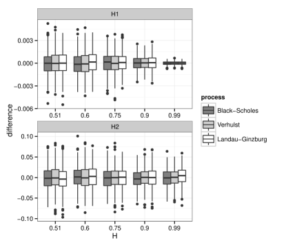
Figure 1: The differences between the estimated and real values of $H$

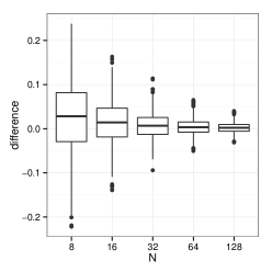
Figure 2: Behavior of $\widehat{H}^{(1)}_{n}$ in case of short sample paths

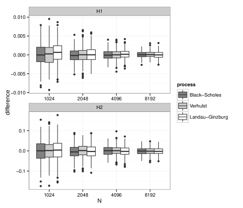
Figure 3: The differences between the estimated and real values of $H$

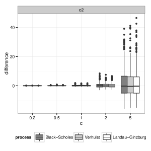
Figure 4: $\widehat{c}^{\,2}_{n}-c^{2}$, dependance on $c$

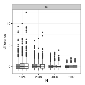
Figure 5: $\widehat{c}^{\,2}_{n}-c^{2}$, dependance on $N$

References

- [1] A. Bégyn, Quadratic variations along irregular partitions for Gaussian processes, Electronic Journal of Probability, 10 (2005), 691–717.
- [2] A. Bégyn, Asymptotic development and central limit theorem for quadratic variations of Gaussian processes, Bernoulli, 13(3) (2007), 712–753.
- [3] A. Benassi, S. Cohen, J. Istas, and S. Jaffard, Identification of filtered white noises, Stochastic Processes and their Applications, 75 (1998), 31–49.
- [4] C. Berzin and J.R. León, Estimation in models driven by fractional Brownian motion, Annales de l’Institut Henri Poincaré, 44 (2008), 191–213.
- [5] J.F. Coeurjolly, Estimating the parameters of a fractional Brownian motion by discrete variations of its sample paths, Statistical Inference for Stochastic Processes, 4 (2001), 199–227.
- [6] R.M. Dudley, R. Norvaiša, Concrete Functional Calculus. Springer Monographs in Mathematics. New York, Springer (2011).
- [7] N.T. Dung, A class of fractional stochastic differential equations, Vietnam Journal of Mathematics, 36(3) (2008), 271-279.
- [8] E. G. Gladyshev, A new Limit theorem for stochastic processes with Gaussian increments, Theory Probab. Appl., 6(1) (1961), 52-61.
- [9] J. Istas, G. Lang, Quadratic variations and estimation of the local Hölder index of a Gaussian process. Ann. Inst. Henri Poincaré, Probab. Stat., 33 (1997), 407-436.
- [10] K. Kubilius, D. Melichov, Quadratic variations and estimation of the Hurst index of the solution of SDE driven by a fractional Brownian Motion, Lithuanian Mathematical Journal, 50(4) (2010), 401-417.
- [11] K. Kubilius, D. Melichov, On comparison of the estimators of the Hurst index of the solutions of stochastic differential equations driven by the fractional Brownian motion, Informatica 22(1) (2011) 97 114.
- [12] K. Kubilius, Y. Mishura, The rate of convergence of estimate for Hurst index of fractional Brownian motion involved into stochastic differential equation, Stochastic Processes and their Applications, 122(11) (2012), 3718-3739.
- [13] K. Kubilius, On estimation of the extended Orey index for Gaussian processes, Stochastics: An International Journal Of Probability And Stochastic Processes.
- [14] R. Malukas, Limit theorems for a quadratic variation of Gaussian processes, Nonlinear Analysis: Modelling and Control, 16 (2011), 435-452.
- [15] R Core Team (2014), R: A language and environment for statistical computing. R Foundation for Statistical Computing, Vienna, Austria. URL http://www.R-project.org/.
- [16] R. Norvaiša, A coplement to Gladyshev’s theorem, Lithuanian Mathematical Journal, 51(1) (2011), 26-35.