Ionized gas at the edge of the Central Molecular Zone

Abstract

Context. The edge of the Central Molecular Zone (CMZ) is the location where massive dense molecular clouds with large internal velocity dispersions transition to the surrounding more quiescent and lower CO emissivity region of the Galaxy. Little is known about the ionized gas surrounding the molecular clouds and in the transition region.

Aims. To determine the properties of the ionized gas at the edge of the CMZ near Sgr E using observations of N⁺ and C⁺.

Methods. We observed a small portion of the edge of the CMZ near Sgr E with spectrally resolved [C ii] 158$\mu$m and [N ii] 205$\mu$m fine structure lines at six positions with the GREAT instrument on SOFIA and in [C ii] using Herschel HIFI on-the-fly strip maps. We use the [N ii] spectra along with a radiative transfer model to calculate the electron density of the gas and the [C ii] maps to illuminate the morphology of the ionized gas and model the column density of CO–dark H₂.

Results. We detect two [C ii] and [N ii] velocity components, one along the line of sight to a CO molecular cloud at -207 km s^-1 associated with Sgr E and the other at -174 km s^-1 outside the edge of another CO cloud. From the [N ii] emission we find that the average electron density is in the range of $\sim$ 5 to 21 cm^-3 for these features. This electron density is much higher than that of the disk’s warm ionized medium, but is consistent with densities determined for bright diffuse H ii nebulae. The column density of the CO–dark H₂ layer in the -207 km s^-1 cloud is $\sim$ 1-2$\times$10²¹ cm^-2 in agreement with theoretical models. The CMZ extends further out in Galactic radius by $\sim$ 7 to 14 pc in ionized gas than it does in molecular gas traced by CO.

Conclusions. The edge of the CMZ likely contains dense hot ionized gas surrounding the neutral molecular material. The high fractional abundance of N⁺ and high electron density require an intense EUV field with a photon flux of order 10⁶ to 10⁷ photons cm^-2 s^-1, and/or efficient proton charge exchange with nitrogen, at temperatures of order 10⁴ K, and/or a large flux of X-rays. Sgr E is a region of massive star formation as indicated by the presence of numerous compact H ii regions. The massive stars are potential sources of the EUV radiation that ionize and heat the gas. In addition X-ray sources and the diffuse X-ray emission in the CMZ are candidates for ionizing nitrogen.

1 Introduction

The Central Molecular Zone (CMZ), the central $\sim$400 pc by $\sim$ 80 pc of the Galaxy, is a region filled with massive dense Giant Molecular Clouds (GMC) having large internal velocity dispersion. Characteristic cloud line widths are $\geq$ 20 km s^-1, compared to a few km s^-1 for GMCs in the disk (e.g. Morris & Serabyn 1996; Oka et al. 1998; Ferrière et al. 2007). In addition, GMCs in the CMZ have higher kinetic temperatures,T${}_{k}\sim$ 30 to 200 K (Ao et al. 2013; Mills & Morris 2013), and densities, n(H₂) $\geq$ 10^4-5 cm^-3 (e.g. Jackson et al. 1996; Oka et al. 1998; Dame et al. 2001; Martin et al. 2004), than GMCs in the disk. The gas distribution within the inner Galaxy and across the edge of the CMZ is thought to be due to the gravitational potential and dynamics of the gas there (see overview by Ferrière et al. 2007). While the atomic and molecular hydrogen distributions in the CMZ have been mapped with spectrally resolved H i and CO, respectively, less is known about the distribution and properties of the ionized gas in this region.

The electron distribution of the interstellar medium has been determined from dispersion measurements of radio emission from pulsars and other compact radio sources (Cordes & Lazio 2002, 2003). Lazio & Cordes (1998) and Roy (2013) find that the average electron density in the inner 100 pc is $<$$n$(e)$>\sim$ 10 cm^-3. The radial distribution has been modeled as a Gaussian with scale length of 145 pc (see Ferrière et al. 2007), which yields a value at the edge of the CMZ $<n$(e)$>\sim$ 1 - 2 cm^-3. Lazio & Cordes (1998) proposed that the scattering of radio waves is not due to a uniform electron distribution but occurs in thin ionized layers at the surface of molecular clouds with $n$(e)$\gtrsim$10³ cm^-3 and T_k(e) $\sim$ 10³ K, or at the interface with the Hot Ionized Medium (HIM) with $n$(e)$\sim$ 5 – 50 cm^-3 and T_k(e) $\sim$ 10⁵ - 10⁶ K. Observations of the spectrally resolved emission from ions in the CMZ can help distinguish among these different models and provide information about the density, filling factor, and ionization mechanisms. The objective of this paper is to explore the nature of the ionized gas at the edge of the CMZ near Sgr E using spectrally resolved emission from the fine structure lines, [N ii] and [C ii], of ionized nitrogen, N⁺, and ionized carbon, C⁺, respectively.

The Balloon-borne Infrared Carbon Explorer (BICE) mapped [C ii] in the inner Galaxy with modest spatial (15^′) and low spectral ($\sim$175 km s^-1) resolution (Nakagawa et al. 1998). BICE detected bright [C ii] emission from the CMZ from 358$\aas@@fstack{\circ}$3 $<l<$ 1^∘ but tapering off outside, and confined to $|b|\lesssim$1^∘ (see their Figures 7 and 8). Within the limitations of BICE’s low spectral resolution, Nakagawa et al. (1998) found that [C ii] has a large velocity dispersion towards the CMZ, $\Delta$v$\geq$100 km s^-1 (see their Figure 14), similar to the dispersion seen in ¹²CO. In addition, the Infrared Space Observatory (ISO) observed [C ii] and [N ii] along a number of lines of sight in the CMZ (see Rodríguez-Fernández et al. 2004) with a spectral resolution $\sim$ 30 km s^-1. However, much better spectral resolution is needed to separate individual components and determine gas characteristics.

To understand better the distribution of the ionized gas at the edge of the CMZ we observed several lines of sight in [N ii] and [C ii] in July 2013 using the heterodyne German REceiver for Astronomy at Terahertz frequencies (GREAT; Heyminck et al. 2012) onboard the Stratospheric Observatory for Infrared Astronomy (SOFIA) (Young et al. 2012). In addition, prior to the GREAT observations, we made small scale strip maps in [C ii] to map the overall distribution of ionized gas as part of a Herschel (Pilbratt et al. 2010) Open Time 2 Programme, using the high spectral resolution Heterodyne Instrument in the Far Infrared (HIFI; de Graauw et al. 2010).

Here we report on the results of these observations, which indicate that there are two regions of highly ionized, high temperature, dense gas: one along the line of sight that includes a CO molecular cloud associated with Sgr E at V${}_{lsr}\sim$ -207 km s^-1 and the other at $V_{lsr}\sim$ -174 km s^-1 outside the edge of a CO molecular cloud located at larger $l$ in the CMZ. The electron densities derived from the [N ii] emission, $n$(e) $\sim$ 5 to 25 cm^-3, are two to three orders of magnitude higher than that in the disk’s warm ionized medium (WIM), but consistent with those found from analysis of [N ii] emission in the Carina Nebula, a luminous H ii region with numerous O stars (Oberst et al. 2011). This paper is organized as follows. In Section 2 we present our observations, while Section 3 analyzes the distribution and density of the ionized gas. Section 4 discusses the possible ionization sources, and Section 5 summarizes the results.

2 Observations of [C ii] and [N ii]

In Figure 1 we show a portion of the NANTEN 4-m CO map from Figure 1a in Fukui et al. (2006), and reprinted with permission from AAAS, that zooms in on the CO edge of the CMZ. The yellow box in Figure 1 outlines the region mapped with HIFI, and the positions observed in [C ii] and [N ii] with GREAT are indicated by red crosses. [N ii] traces just the highly ionized gas, while [C ii] traces highly ionized gas and the weakly ionized neutral atomic and molecular gas. Located just inside the edge of the CMZ is Sgr E, a region with many radio sources located around $l\sim$ 358$\aas@@fstack{\circ}$7 and $b\sim$ 0^∘ (Gray 1994), which contains 18 compact ($<$2^′) H ii regions and diffuse emission (Liszt 1992). Sgr E is a region of active star formation associated with a CO molecular cloud with V${}_{lsr}\sim$ -210 km s^-1 (Oka et al. 1998). The radio recombination line survey, H ii Region Discovery Survey (HRDS: Anderson et al. 2011, 2012) detected eight of these H ii sources towards Sgr E at $V_{lsr}\sim$ -208 km s^-1, the same velocity as the CO cloud. Along the line of sight outside the CMZ there are Giant Magnetic Loops, large scale molecular gas loop-like features, with large line widths and large scale flows detected in CO (Fukui et al. 2006; Fujishita et al. 2009). The edge of Loop 1 intercepts the plane at $l\sim$358$\aas@@fstack{\circ}$2 to 358$\aas@@fstack{\circ}$4, close to the line of sight to the edge of the CMZ, and has a V${}_{\rm lsr}\sim$ -135 km s^-1 (Fukui et al. 2006). This loop, however, is at a Galactic radius, R${}_{G}\sim$670 pc (Torii et al. 2010), well outside the CMZ.

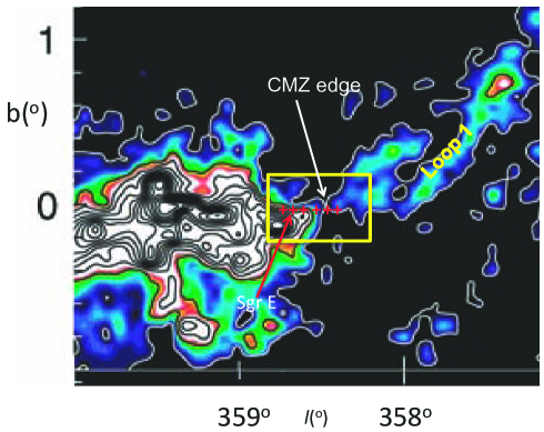
Figure 1: A portion of a map of CO integrated intensity from -180 to -90 km s^-1 of the edge of the CMZ from (Fukui et al. 2006), and reprinted with permission from AAAS, based on the NANTEN CO(1-0) map which has a beam size $\sim$3^′. The region mapped with HIFI is outlined by the yellow box and the positions of the [C ii] and [N ii] observations with GREAT are indicated by crosses. The approximate CO edge of the CMZ and a portion of Loop 1 are indicated, as is the location of Sgr E.

2.1 SOFIA [C ii] and [N ii] data

We observed the lower fine structure transition of ionized nitrogen, [N ii] ${}^{3}P_{1}$$\rightarrow$${}^{3}P_{0}$ at 1461.1319 GHz (205.2 $\mu$m) and, simultaneously, the fine structure line of ionized carbon, [C ii] ${}^{2}P_{3/2}$$\rightarrow$${}^{2}P_{1/2}$ at 1900.5369 GHz (157.7 $\mu$m), using GREAT. The angular resolution is 15^′′ at [C ii] and 20^′′ at [N ii]. To improve the signal-to-noise ratio (SNR) the [C ii] and [N ii] data were smoothed to a velocity resolution of 1.20 km s^-1 and 1.57 km s^-1 per channel, respectively. The spectra were calibrated using the procedure outlined in Guan et al. (2012).

The GREAT [C ii] observations contained atmospheric features in the spectral region observed due to the frequency setting for large negative velocities of the source, and the [C ii] line was in the wing of a strong water line. Moreover, the position switching observing mode made the presence of this feature a significant issue that needed to be addressed in the data reduction. The standard atmospheric calibration was not sufficient to produce a satisfactory fit to the water feature, and we had to use a set of non-standard parameters in the atmospheric model (Guan et al. 2012) to fit the width and the peak of the water line. The main change to the normal procedure was to reduce the contribution from the Dry atmosphere in steps, allowing the Wet part (water) to fit the atmospheric feature. We implemented a set of six models, and chose the model that best fit the water feature. This feature was removed and a zero order spectral baseline fit applied to the delivered data products. The resulting spectra were, with one exception, fairly regular with residual low order polynomial variations and only slight offsets from zero; one spectrum had a long period, but well ordered, variation in the baseline. In order to fit the baselines better than zero order, the delivered data were then reduced further in CLASS and baselines corrected with a polynomial fitting routine. Comparison of the GREAT and HIFI [C ii] data at one nearly coincident position (see below) shows excellent agreement, lending confidence to the removal of the water line and overall baseline fittings. The intensities were corrected for a main beam efficiency of 0.67. The rms noise for the final [C ii] products ranges from 0.16 to 0.26 K per 1.20 km s^-1 channel, while that for [N ii] ranges from 0.09 to 0.23 K per 1.57 km s^-1 channel.

We observed six lines of sight (LOS) along $b$=0^∘ at longitudes from $l$=358$\aas@@fstack{\circ}$45 to 358$\aas@@fstack{\circ}$75. The reference off-position, OFF1, $l$=358$\aas@@fstack{\circ}$50 and $b$=0$\aas@@fstack{\circ}$25 contains weak [C ii] and very weak [N ii] emission, shown in Figure 2, so that all the on-positions had to be corrected for this emission. To correct the observations for emission in OFF1 it was observed separately on two nights as an on-position using a different off-position, OFF2, $l$=358$\aas@@fstack{\circ}$50 and $b$=0$\aas@@fstack{\circ}$65. The OFF1 lines appear to be singly peaked and a Gaussian fit to the [C ii] emission in OFF1 peaks at V${}_{lsr}\sim$ -195 km s^-1 and has a full width half maximum (FWHM) $\sim$ 43 km s^-1. The narrow [C ii] feature at V${}_{lsr}\sim$ -58 km s^-1 (FWHM $\sim$ 9 km s^-1) arises from the 3 kpc arm. A Gaussian fit to the broad, weak [N ii] line yields a peak V${}_{lsr}\sim$ -205 km s^-1 and a FWHM $\sim$65 km s^-1, close to the characteristics of the [C ii] line considering the weakness of the line and the low signal-to-noise ratio of this detection. No other [N ii] is detected in the band above the 3-$\sigma$ level.

As a check on the quality of the GREAT data, given that it had to be corrected for the atmospheric water line and emission in the OFF1 position, we show in Figure 3 a spectrum from the HIFI Galactic Observations of Terahertz (GOT C+) [C ii] survey (Langer et al. 2010; Pineda et al. 2013) at the closest position, $l=$358$\aas@@fstack{\circ}$696 and $b=$0$\aas@@fstack{\circ}$0, to the GREAT observation at $l=$358$\aas@@fstack{\circ}$700 and $b=$0$\aas@@fstack{\circ}$0. The offset in longitude of 14^′′ corresponds to 1.2 HIFI and 0.9 GREAT beam widths, and some portions of the main beams are only about an arcsecond apart. The [C ii] emission from HIFI and GREAT have the same distribution in velocity, both show a strong peak at $\sim$ -210 km s^-1 with intensities that generally agree within the uncertainties of the baseline fitting, and both show weak emission centered around $\sim$ -175 km s^-1 that blends into the stronger feature. The integrated intensities of these two observations over the velocity range -150 km s^-1 to -250 km s^-1 differ by only 10%. Furthermore, the GOT C+ spectrum used a different off position than the GREAT observations, lending further support for our procedure to correct the GREAT [C ii] and [N ii] for emission in the GREAT OFF1 position.

The [C ii] and [N ii] spectra along $b$=0^∘ are shown in Figure 4. [C ii] emission was detected at all six positions and there are two adjacent, and at times blended, features arising from the CMZ in the velocity range $\sim$-150 km s^-1 to -250 km s^-1. At the two positions where these components are clearly separated, the peaks occur at V${}_{lsr}\sim$ -174 and -207 km s^-1. In general the -174 km s^-1 component is weaker than the -207 km s^-1 component, and both features are broad with a typical FWHM of $\sim$ 25 km s^-1. No emission is detected at V_lsr$\sim$ -135 km s^-1, the velocity of Loop 1.

[N ii] is only detected at four of the six LOS, and is generally much weaker than [C ii] except at $l$=358$\aas@@fstack{\circ}$45 where the component at V${}_{lsr}\sim$ -207 km s^-1 is about half as intense as [C ii]. The four LOS where [N ii] is detected have an rms noise of $\sim$0.1 K per 1.57 km s^-1 channel whereas the two lines of sight where [N ii] is not detected have a larger rms noise, $\sim$0.23 K. The [N ii] components were fit with a double Gaussian with one peak at $\sim$ -215 km s^-1 and a FWHM $\sim$35 km s^-1 and the other component is at $\sim$ -170 km s^-1 with a FWHM $\sim$25 km s^-1. All the [C ii] features have a large SNR while the [N ii] SNR ranges from $\sim$4 to 20 for the four LOS in which the line was detected.

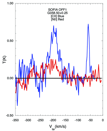
Figure 2: [C ii] and [N ii] emission in the reference OFF1 position at $l$=358$\aas@@fstack{\circ}$50 and $b$=0$\aas@@fstack{\circ}$25. The data have been smoothed to 2.4 km s^-1 for [C ii] and 3.1 km s^-1 for [N ii] to improve the signal-to-noise. The [C ii] emission peaks at V${}_{lsr}\sim$ -195 km s^-1 while that from [N ii] peaks $\sim$ -207 km s^-1, within the fitting errors of the weaker [N ii] signal. The narrow [C ii] emission at V${}_{lsr}\sim$ -58 km s^-1 arises from the 3 kpc arm. [N ii] is not detected from this arm.

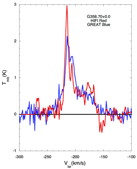
Figure 3: GREAT [C ii] spectrum at the position observed with GREAT, $l$=358$\aas@@fstack{\circ}$700 and $b$=0$\aas@@fstack{\circ}$0, that is closest to a [C ii] spectrum from GOT C+. The GOT C+ position $l=$358$\aas@@fstack{\circ}$696 and $b=$0$\aas@@fstack{\circ}$0 is offset in longitude by 14^′′ from the GREAT pointing, which is about the GREAT beam width. The HIFI data have been smoothed to the resolution of the GREAT data, 1.2 km s^-1. The [C ii] GREAT spectrum is similar to that from HIFI showing both the -207 km s^-1 and -174 km s^-1 components. The total integrated intensities agree within $\pm$10%.

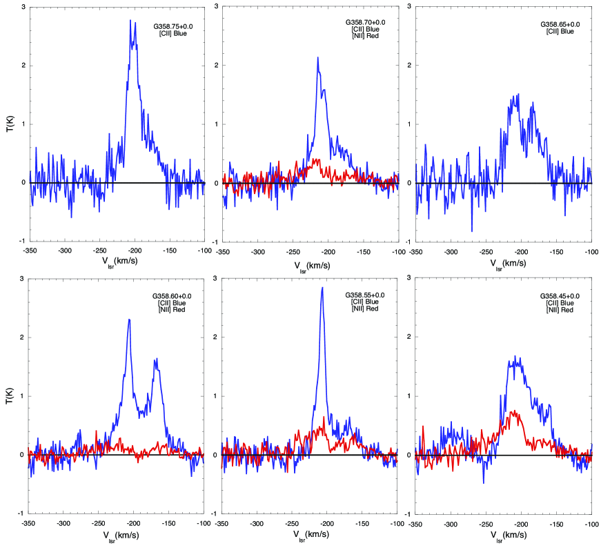
Figure 4: [C ii] (blue) and [N ii] (red) spectra at the six positions observed with GREAT along $b$=0$\aas@@fstack{\circ}$0. The Galactic longitude and latitude are indicated by GXXX.XX+Y.Y. The two features centered at $\sim$ -174 km s^-1 and $\sim$ -207 km s^-1(which are blended at some positions) arise from the edge of the CMZ. [C ii] is detected at all 6 positions in the CMZ, but [N ii] is only detected at 4 positions. The two non-detections in [N ii] are associated with greater rms noise. While [N ii] is generally much weaker than [C ii], the [N ii] peak temperature at $l$=358$\aas@@fstack{\circ}$45 is about half that of [C ii].

2.2 Herschel [C ii] map data

The GREAT observations provide [C ii] at six and [N ii] at four longitudinal positions in the plane ($b=$ 0^∘). To get insight into the distribution of [C ii] above and below the plane we use [C ii] maps made with the high spectral resolution HIFI (de Graauw et al. 2010) instrument onboard Herschel (Pilbratt et al. 2010). We used a number of On-The-Fly (OTF) scans to map the 0$\aas@@fstack{\circ}$6 $\times$ 0$\aas@@fstack{\circ}$4 region shown in Figure 1. All HIFI OTF scans were made in the LOAD-CHOP mode using a reference off-source position at $l$=358$\aas@@fstack{\circ}$80, $b$=1$\aas@@fstack{\circ}$90, about 1$\aas@@fstack{\circ}$7 away in latitude from the top of the map. The map consists of 13 scans in Galactic latitude, centered at $b$ = 0^∘ and stepping in longitude at 3^′ (0$\aas@@fstack{\circ}$05) intervals from 358$\aas@@fstack{\circ}$20 to 358$\aas@@fstack{\circ}$80. The OTF $b$-scans are 24^′ long, sampled at every 40 ^′′. At 1.9 THz the angular resolution of the Herschel telescope is 12^′′, corresponding to a spatial resolution of $\sim$0.5 pc at 8.5 kpc, the distance to the Galactic Center. However the effects of scanning rate and the 40^′′ sampling of the OTF maps degrades the effective resolution in $b$ to 80^′′ while it is 12^′′ in $l$. Thus spatial structures on scale sizes smaller than 80^′′ in $b$ will be strongly attenuated. Furthermore the total duration of each OTF scan was typically $\sim$2000 sec which provides only a small integration time on each spectrum (pixel). Thus the rms in the OTF spectra, 0.22 K in T_mb in an 88^′′ beam and 3 km s^-1 channel, is larger than that in the corresponding GREAT spectra.

The OTF map data presented here were processed following one of the procedures suggested by the Herschel Science Center science staff, by running the HIPE pipeline without an off-source subtraction to produce level 1 data. Then the hebCorrection routine was applied to the level 1 data to remove the HEB standing waves and afterwards we followed the procedure described in Velusamy & Langer (2014) to produce the level 2 data and spectral line maps. The fact that hebCorrection subtracts the matching standing wave patterns from a large database of spectra eliminates the need for off-source subtraction. Thus in our analysis the processed spectral data are free from any off source contamination. We use the processed spectral line scan map data to make latitude–velocity ($b$–V) maps of the velocity structure of the [C ii] emission as a function of latitude at each of the 13 longitudes of the OTF positions. To increase the sensitivity of the $b$–V maps we use a velocity resolution of 3 km s^-1. In all the OTF $b$–V maps the velocity feature near -207 km s^-1 is prominent, but that of the weaker -174 km s^-1 feature is less so, possibly due to the combined effect of low sensitivity and beam dilution. However, the bright [C ii] features ($>$ 1K) are well traced in the OTF maps. To bring out the spatial structure of the -207 km s^-1 velocity feature we generate a [C ii] integrated intensity map covering -220 km s^-1 to -200 km s^-1. This velocity range facilitates comparison with the Nobayama CO maps of Oka et al. (1998), which are presented in 10 km s^-1 intervals. To generate the [C ii] map we integrate the intensities in the $b$–V maps at each latitude pixel over the range of velocities from -220 km s^-1 to -200 km s^-1 around the [C ii] spectral peak. We then use these intensities at all longitudes to generate the 2–D map shown in Figure 5. Note that while the intensities are sampled contiguously in latitude, we only have data at 13 discrete longitudes with a pixel width of 12^′′. To make the data more visible on the map we broadened their display in longitude to 60^′′. There is little or no [C ii] for $l<$ 358$\aas@@fstack{\circ}$30.

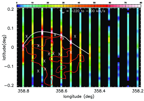
Figure 5: Comparison of the [C ii] OTF intensity maps integrated over the velocity range -220 km s^-1 to -200 km s^-1 shown as coulored strips with the CO map from Oka et al. (1998) integrated over the velocity range -220 to -210 km s^-1. The CO integrated intensity maps from Oka et al. (1998) are shown only in 10 km s^-1 steps, but to improve the signal to noise in the [C ii] OTF maps we use a range of 20 km s^-1. The CO map integrated from -210 to -200 km s^-1 shows the same extent in $b$ and the same edge at $l\sim$ 358$\aas@@fstack{\circ}$5 as the -220 to -210 km s^-1 map, but extends further to 359$\aas@@fstack{\circ}$0, and would give the same morphological relationship to the [C ii] contours. The color bar at the top indicates the [C ii] integrated intensity in K km s^-1. The [C ii] OTF maps sample in $b$ every 0$\aas@@fstack{\circ}$05 in longitude from 358$\aas@@fstack{\circ}$2 to 358$\aas@@fstack{\circ}$8, so generating a contour map is impractical due to the sparse sampling in $l$. Instead we have indicated by the white line the connection of the peak intensity in each strip. The CO contours, indicated in red, are in steps of 15 K km s^-1. The [C ii] is strongest slightly beyond the edge of the CO emission above the plane. The compact H ii sources towards Sgr E (Liszt 1992) are indicated by white and red X symbols, depending on background colour.

3 Results

The relationship between the distribution in [C ii] and CO is brought out in Figure 5 where we superimpose on the [C ii] strip maps the CO integrated intensity from -210 km s^-1 to -220 km s^-1 (Oka et al. 1998). The only caveat is that the region at the edge of the CMZ is irregularly mapped in CO in the Nobayama maps. However, the AT&T Bell Labs CO survey mapped the CMZ out to $l=\pm$2^∘ (see Figure 1; Morris & Serabyn 1996) and also shows a sharp edge in CO emission at $l\sim$358$\aas@@fstack{\circ}$5. The -207 km s^-1 cloud is clearly seen in the position-velocity maps from the AT&T Bells Labs CO survey (see Figure 4; Morris & Serabyn 1996). The CO emission comes from the cloud associated with Sgr E, an active region of star formation with bright compact H ii regions. Though our [C ii] map is not contiguous in longitude (scans are spaced by 3^′) the brightest emission (white in the color wedge) appears to be an arc above the plane slightly outside the lowest CO contour. The [C ii] arc is most likely limb brightened emission. There does not appear to be a similar limb brightening for $b<$0^∘. Although we do not have any [N ii] observations along this arc, we conclude from the presence of [N ii] along the line of sight to the CO cloud at $b$ = 0^∘ that the [N ii] and [C ii] emission arise from an ionized region surrounding the cloud, but there is also a likely contribution to [C ii] from a photon dominated region (PDR) sandwiched between the highly ionized hydrogen and dense molecular gas traced by CO. Also indicated on the map are 15 of the 18 compact H ii sources detected by Liszt (1992) towards Sgr E (the remaining three are outside the mapped region). In addition to these compact H ii regions there appears to be low level diffuse emission from $l\sim$ 358$\aas@@fstack{\circ}$8 to 359$\aas@@fstack{\circ}$0 between $b=\pm$0$\aas@@fstack{\circ}$1 (see Figure 8 in Liszt (1992)). The compact H ii sources have electron densities of order several hundred cm^-3 and require ionizing stars of type B0 or brighter (Liszt 1992).

All six [C ii] and the four [N ii] spectra in Figure 4 show emission in the velocity range -140 to -240 km s^-1. The detection of broad emission in [C ii] and [N ii] indicates the presence of warm, and perhaps dense, ionized gas at the edge of the CMZ. To gain further insight into the nature of the gas and its association with different interstellar medium (ISM) components we compare [C ii] and [N ii] to the CO(1-0) and H i spectra along $b=$ 0^∘ taken from the Three-mm Ultimate Mopra Milky Way Survey (ThrUMMS) (Barnes et al. 2011) and the Australia Telescope Compact Array H i Galactic Center survey (McClure-Griffiths et al. 2012), respectively.

In Figure 6 we plot the CO(1-0) spectra at $b=$ 0^∘ along the strip observed with GREAT, $l=$ 358$\aas@@fstack{\circ}$40 to 358$\aas@@fstack{\circ}$75 and $b=$ 0^∘. The corresponding H i spectra are plotted in Figure 7. The CO and H i spectra show that there are two different environments detected in [C ii] and [N ii]. The emission at V${}_{lsr}\sim$ -207 km s^-1 is associated with both CO and H i, while that for -174 km s^-1 is associated only with H i until $l\sim$ 358$\aas@@fstack{\circ}$75, where there is a hint of CO emission. The distributions of the [C ii] and [N ii] emission for the -207 km s^-1 component are towards the edge of a CO molecular cloud associated with Sgr E, while the -174 km s^-1 distribution is along the edge of another CO molecular cloud, as can be seen in the Nobayama CO maps in this velocity range (Oka et al. 1998).

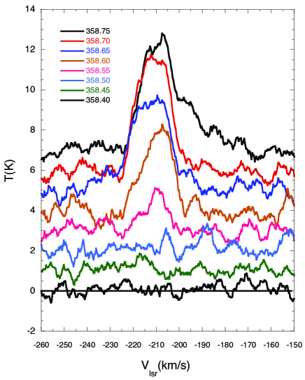
Figure 6: CO(1-0) spectra at $b=$ 0^∘ at the longitudes observed in [C ii] and [N ii]. The data is taken from the ThrUMMS survey (uncorrected for main beam efficiency) and the inset is a key to the lines of sight observed. Moving towards the CMZ, larger $l$, CO is not detected until $l\sim$ 358$\aas@@fstack{\circ}$55 (although there is a hint of CO at 358$\aas@@fstack{\circ}$50) at the inner edge of the CMZ, and that only the -207 km s^-1 component is present. The -174 km s^-1 CO component is detected at 358$\aas@@fstack{\circ}$75, the position furthest from the edge of the CMZ and it is considerably weaker there than the -207 km s^-1 component.

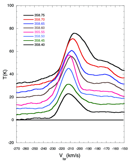
Figure 7: H i spectra at $b=$ 0^∘ along the latitudes observed in [C ii] and [N ii]. The data are taken from the ATCA H i survey (McClure-Griffiths et al. 2012) and the inset is a key to the lines of sight observed. H i is detected at all positions at -207 km s^-1 and is strongest close to Sgr E. H i is also detected at -174 km s^-1 but is weaker than at -207 km s^-1.

To evaluate the properties of the ionized gas we derived the parameters of the [C ii], [N ii], and CO from Gaussian fits to each line component. In cases where the lines are blended we derive their line parameters using a double Gaussian fit over the velocity range -100 km s^-1 to -300 km s^-1. The intensities are given in Table 1. We calculate the corresponding H i intensities by integrating over the velocity ranges of the two [C ii] components because we cannot get unambiguous Gaussian fits over such broad and, at low velocities, flat lines. To avoid double counting the intensities we chose -190 km s^-1 as the dividing velocity of the two components, and their intensities are given in Table 1. In general, there is a good correlation of [N ii] intensity with [C ii] intensity, which suggests that a significant fraction of the [C ii] emission arises in the [N ii] region. We will use the [C ii] and [N ii] integrated intensities to characterize the properties of the ionized gas.

Table 1: Integrated line intensities

LOS	I([C ii])a,b	I([N ii])c	I(CO)	I(H i)
Vlsr = -207 km s-1
358.45+0.0	63.4	26.4	6.7	1047
358.55+0.0	45.4	15.4	26.6	1904
358.60+0.0	47.6	7.1	60.6	2189
358.65+0.0	38.6	-	101.9	2539
358.70+0.0	45.4	12.4	98.9	2923
358.75+0.0	57.4	-	110.5	3235
Vlsr = -174 km s-1
358.45+0.0	21.1	8.2	-	730
358.55+0.0	12.2	8.8	-	1212
358.60+0.0	43.0	3.7	-	1544
358.65+0.0	25.5	-	-	1855
358.70+0.0	15.3	5.3	-	2177
358.75+0.0	21.8	-	9.8	2522

a) Integrated intensities are in units of K km s^-1. We only report detections with a SNR $\geq$ 3, see text. b) Typical rms noise in the [C ii] integrated intensity is $\sim$1.4 K km s^-1. c) Typical rms noise in the [N ii] ntegrated intensity is $\sim$1.3 K km s^-1.

3.1 Radiative transfer solutions for [C ii] and [N ii]

The relationship of the column density of C⁺ and line intensity, I([C ii]), has been extensively discussed in the literature (e.g. Goldsmith et al. 2012). The [C ii] peak antenna temperatures reported here are $<<$0.3 times the kinetic temperature and, as discussed by Goldsmith et al. (2012), are in the “effectively optically thin limit” in which the column density is proportional to the integrated line intensity. Therefore we have from Langer et al. (2014), Equation A.2, the relationship between the column density, $N$(C⁺) in cm^-2 and integrated line intensity, $\int T(K)d\rm{v}$, in K km s^-1,

$$N(C^{+})=2.92\times 10^{15}[1+0.5e^{\Delta E/kT}(1+\frac{n_{cr}}{n})]I([C\,II])\,\,\rm{cm^{-2}}$$ (1)

where $\Delta E/k$ =91.25K is the energy needed to excite the ${}^{2}P_{3/2}$ level, $n$ is the density of the collision partner of the bulk of the gas, and $n_{cr}$ is the corresponding critical density. The collision rate coefficients for e, H, and H₂ are summarized in Goldsmith et al. (2012) with an update for H₂ in Wiesenfeld & Goldsmith (2014). Electrons will dominate the excitation of C⁺ where we detect [N ii]. In the ionized regions where [N ii] is detected the temperatures are high enough that we can neglect the exponential term and

$$N(C^{+})=2.92\times 10^{15}[1+0.5(1+\frac{n_{cr}(e)}{n(e)})]I([C\,II])\,\,\rm{cm^{-2}}.$$ (2)

The relationship of the column density of ionized nitrogen to the integrated line intensity, in units of K km s^-1, in the optically thin limit, assuming uniform excitation along the line of sight, is given by,

$$I_{ul}([N\,II])=\int T_{ul}(K)d{\rm v}=\frac{hc^{3}}{8\pi k(\nu_{ul})^{2}}A_{ul}f_{u}N(\rm{N}^{+})\,\rm{cm^{-2}},$$ (3)

where $A_{ul}$ is the Einstein A-coefficient, $\nu_{ul}$ the transition frequency, $f_{u}$ is the fractional population of the upper state which depends on the density of the collision partner, $n$, $I$ is in units of K km s^-1, and $N$(N⁺) is the column density of ionized nitrogen. For the ${}^{3}P_{1}\rightarrow$ ${}^{3}P_{0}$ transition at 205 $\mu$m this equation reduces to

$$I([N\,II])=5.06\times 10^{-16}f_{1}N(\rm{N}^{+})\,\,\rm{(K\,km\,s^{-1})}$$ (4)

where $f_{1}$ is the fractional population of N⁺ in the ${}^{3}P_{1}$ state. If we assume that the [N ii] emission region is uniform we can replace $N$(N⁺) by, $n$(N⁺)$L$, where $L$ is the path length in cm,

$$I([N\,II])=5.06\times 10^{-16}f_{1}n(\rm{N}^{+})L\,\,\rm{(K\,km\,s^{-1})}$$ (5)

We can solve for $f_{1}$ in the optically thin limit from the detailed balance equations for the ³P₂, ³P₁, and ³P₀ states along with the condition $f_{0}+f_{1}+f_{2}=$1. In ionized regions electrons dominate the excitation of N⁺. The collisional de-excitation rate coefficient by electrons is given by

$$C_{ul}=8.63\times 10^{-6}\frac{G(u,l)}{g_{u}T^{0.5}},$$ (6)

where $g_{u}$ is the degeneracy of the upper level and $G(u,l)$ is the temperature dependent effective collision strength (see Lennon & Burke 1994; Hudson & Bell 2004). We calculated the electron collisional rate coefficients using the Hudson & Bell (2004) values for the effective collision strengths. The critical density for the 1-0 transition, where collisions out of the ${}^{3}P_{1}$ state balance the radiative transition, A₁₀, is $n_{cr}$(e) $\sim$ 44 cm^-3 at 8000K. In Figure 8 we plot the intensity of the 205 $\mu$m line as a function of the electron density using Equation 4 for a range of ionized nitrogen column densities, $N$(N⁺) = 10¹⁶ to 10¹⁸ cm^-2. The intensity scales linearly with $n$(e) up to $\sim$10 - 15 cm^-3 beyond which it levels off as $n$(e) approaches the critical density.

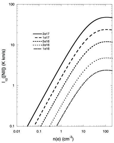
Figure 8: The intensity of [N ii] 205 $\mu$m line versus $n$(e) for a range of ionized nitrogen column densities; the insert gives the key for the column density. The curves flatten out as the density approaches the critical density.

The [N ii] emission comes from ionized gas and so can be used to derive the electron density directly if we know the size of the emitting region and the fractional abundance of ionized nitrogen, $x$(N⁺) = $n$(N⁺)/$n_{t}$, where $n_{t}$= $n$(H)+2$n$(H₂)+$n$(H⁺) is the total density of hydrogen nuclei including ions. To estimate $n($e) we replace the density of ionized nitrogen, $n$(N⁺), in Equation 5 by $x$(N⁺)$n_{t}$, and because the [N ii] emission arises from highly, or perhaps completely, ionized gas we set $n_{t}\simeq n$(H⁺) = $n$(e). For a uniform density region we can take $N$(e) = $n$(e)$L$, where $L$ is the thickness of the emission region, and can now express Equation 5 as

$$I([N\,II])=\int T_{10}dv=5.06\times 10^{-16}x(N^{+})Ln(e)f_{1}(n(e)),$$ (7)

where $I$ is in K km s^-1. Rewriting in convenient units we obtain,

$$I([N\,II])=0.156x_{-4}(N^{+})L_{pc}n(e)f_{1}(n(e)),$$ (8)

where $x_{-4}$ is the fractional abundance of N⁺ is in units of 10^-4 and $L_{pc}$ is in pc. Thus we can solve for the electron density, $n$(e), as a function of the observed intensity of the 205 $\mu$m line, given the size of the emission region and the fractional abundance of N⁺. At low densities, where $n$(e)$<n_{cr}$(e), it can be shown that

$$n(e)\propto\left[\frac{I(N\,II)}{L_{pc}x_{-4}(\rm{N^{+}})}\right]^{\alpha}\,\,\rm{cm^{-3}}$$ (9)

where $0.5<\alpha<0.7$, for $n$(e)$<n_{cr}$(e). In the limit $n$(e)$<<n_{cr}$(e), such as found in the Warm Ionized Medium in the disk, $f_{1}\sim n$(e)/$n_{cr}$(e) and $\alpha=$0.5. Thus, in general, $n$(e) is only moderately sensitive to uncertainties in $L$ and $x$(N⁺).

3.2 The -207 km s^-1 component

As seen in Figures 4 and 5 there is [C ii] emission along the line of sight to the CO molecular cloud with V${}_{lsr}\sim$ -207 km s^-1. The peak in [C ii] intensity for this component is at $b>$ 0^∘ at the edge of the lowest contour of CO and is thus consistent with limb brightened [C ii] emission. Therefore the SOFIA [C ii] and [N ii] spectra along $b$=0^∘ likely arise from a layer of gas whose size is related to the thickness of the [C ii] emission beyond the lowest CO contour. The thickness of the [C ii] emission is about 6^′ which corresponds to $\sim$15 pc at the distance to the CMZ. To solve for the electron abundance in the [N ii] regions we need, in addition to $L_{pc}$ and $I($[N ii]$)$, $x(\rm{N}^{+})$ appropriate to the CMZ. To estimate the fraction of N⁺ in the CMZ we use the nitrogen abundance Galactic gradient, 0.07 dex kpc^-1, for $R_{G}>$ 3 kpc, derived from Rolleston et al. (2000) which leads to $x($N⁺) $\propto exp(-R_{G}/6.2)$ (see Pineda et al. 2013; Langer et al. 2014). However because we do not have information about how it scales to smaller $R_{G}$ we extrapolate this relationship to the half way point, 1.5 kpc. Using the local nitrogen abundance fraction $x(N^{+})$ =5.51$\times$10^-5 from Jensen et al. (2007) yields $x$(N⁺) = 1.6$\times$10^-4 at R_G=1.5 kpc. As discussed above, the solutions for $n$(e) are not very sensitive to modest uncertainties in $x$(N⁺). The solutions for $n$(e) and $N$(N⁺) are given in Table 2.

The electron density for the -207 km s^-1 component varies from $\sim$9 to 21 cm^-3 for the four LOS with [N ii] detections and has an average value $\sim$14 cm^-3. Thus the gas traced by [N ii] is warm dense ionized gas, significantly denser than that derived for the typical WIM in the disk, which has $n$(e) of order a few$\times$10^-2 cm^-3 (Haffner et al. 2009; Velusamy et al. 2012). In the next section we will discuss what might generate and sustain such a high density ionized gas towards the cloud associated with Sgr E.

Table 2: Electron density and nitrogen column density

Vlsra =	-207	-207	-207	-174	-174	-174
LOS	$n$(e)b	$N$(N+)c	$N$(H+)	$n$(e)b	$N$(N+)	$N$(H+)
358.45d	20.7	1.5e17	9.3e20	9.9	7.5e16	4.6e20
358.55	14.6	1.1e17	6.8e20	10.4	7.9e16	4.8e20
358.60	9.1	6.9e16	4.2e20	6.3	4.8e16	2.9e20
358.65	-	-	-	-	-	-
358.70	12.8	9.7e16	5.9e20	7.7	5.9e16	3.6e20
358.75	-	-	-	-	-	-
Average	14.3	1.1e17	6.6e20	8.6	6.5e16	4.0e20

a) In km s^-1. b) Densities in cm^-3. c) Column densities in cm^-2 and rounded to one decimal place. d) All LOS are along $b=$0^∘.

Assuming that the nitrogen is nearly fully ionized, the column density of ionized carbon in this region is given by $N$(C⁺)=$x$(C⁺)/$x$(N⁺)$N$(N⁺). For $x($C⁺)/$x$(N⁺) we adopt the value of 3.2 (Jensen et al. 2007; Sofia et al. 2004) and the values for N(C⁺) are given in Table 3 along with $N$(H⁺). The C⁺ column densities are of order a few$\times$10¹⁷ cm^-2, with an average $\sim$4$\times$10¹⁷ cm^-2.

The [C ii] intensity associated with the [N ii] region, $I_{\rm{H}^{+}}$([C ii]), is calculated using the inverse of Equation (2), from the column density $N$(C⁺), $n$(e) derived from [N ii], and assuming T_k = 8000 K. The exact kinetic temperature is not critical as the column density is only weakly dependent on temperature through the collisional de-excitation rate coefficient, resulting in $n_{cr}$(e) $\sim$ 50$T_{4}$^0.37 cm^-3, where $T_{4}$ is the kinetic temperature in units of 10⁴ K. The results are given in Table 3.

The [C ii] emission from the neutral PDR, $I_{\rm{H_{2}}}$([C ii]), is the difference between the observed total [C ii] intensity, $I$([C ii]), given in Table 1, and the intensity calculated from the [N ii] region, $I_{\rm{H^{+}}}$([C ii]) (Langer et al. 2014). This quantity, $I_{\rm{H_{2}}}$([C ii]) = $I$([C ii]) - $I_{\rm{H^{+}}}$([C ii]) arises primarily from the CO–dark H₂ gas (also called the CO–dark gas) and is given in Table 3. Negative or very small values of $I_{\rm{H_{2}}}$([C ii]) indicate that almost all the [C ii] emission arises from the dense ionized gas. Unfortunately we do not know the kinetic temperature and hydrogen density of the CO–dark $N$(H₂) to calculate accurately its measured C⁺ column density. For illustrative purposes we calculate the column density of C⁺ in the H₂ layer, $N_{\rm{H_{2}}}$(C⁺), and the corresponding column density of CO–dark H₂, $N_{\rm C^{+}}$(H₂)= $N_{\rm{H_{2}}}$(C⁺)/$x$(C⁺) (see Langer et al. 2014), assuming 100K and 300 cm^-3 in Equation (1), along with the appropriate $n_{cr}$(H₂) from Wiesenfeld & Goldsmith (2014). These results are listed in Table 3 for all the LOS with positive $I_{\rm{H_{2}}}$([C ii]). Higher densities will result in lower column densities and vice versa.

Table 3: C⁺ column densities and intensities

LOSa	$N$(C+)b	$I_{\rm{H^{+}}}$([C ii])c	$I_{\rm{H_{2}}}$([C ii])	$N_{\rm{H_{2}}}$(C+)	$N_{\rm{C^{+}}}$(H2)f
-207d
358.45	4.9e17	64.1	-0.7	-	-
358.55	3.5e17	38.5	7.0	4.2e17	8.2e20
358.60	2.2e17	18.3	29.3	1.8e18	3.5e21
358.65	-	-	-	-	-
358.70	3.0e17	31.3	14.1	8.6e17	1.7e21
358.75	-	-	-	-	-
Average	3.4e17	38.1	16.8e	1.0e18	2.0e21
-174d
358.45	2.4e17	21.1	0.1	3.3e15	6.4e18
358.55	2.5e17	22.6	-10.4	-	-
358.60	1.5e17	9.9	33.1	2.0e18	3.9e21
358.65	-	-	-	-	-
358.70	1.8e17	13.4	1.3	8.2e16	1.6e20
358.75	-	-	-	-	-
Average	2.0e17	16.9	11.5e	7.0e17	1.4e21

a) All LOS are at $b=$0^∘. b) Column density in cm^-2 and rounded to one decimal place. c) Intensity of [C ii] in the [N ii] emission region in K km s^-1. d) V_lsr in km s^-1. e) Negative intensities are not included. f) Assumes $T_{k}$=100 K and $n$(H₂) = 300 cm^-3.

3.3 The -174 km s^-1 component

The -174 km s^-1 [N ii] and [C ii] emissions are weaker, and in some positions much weaker, than those of the -207 km s^-1 component, and are associated with CO only at $l=$358$\aas@@fstack{\circ}$75 in Figure 6. The CO maps in Oka et al. (1998) show a CO molecular cloud with an edge at this longitude and extending inwards to larger $l$. The -174 km s^-1 emission is also associated with H i emission (Figure 7) that is weaker than that of the -210 km s^-1 cloud. We do not detect this weaker [C ii] component at all the positions in the HIFI OTF maps (see discussion in Section 2.2) and so have no estimate of the size of the [C ii] and [N ii] emission region. For comparison we have calculated densities and the column densities of this component assuming the same size, 15 pc, for the [N ii] emission region as that for the -207 km s^-1 cloud. These results are given in Tables 2 and  3. The solutions for the -174 km s^-1 component yield slightly lower average electron densities and column densities than for the -207 km s^-1 component.

4 Discussion

The analysis of [N ii] emission at the edge of the CMZ reveals a hot dense plasma with an electron abundance ranging from $\sim$ 6 to 21 cm^-3. The densities we derive are much larger than those characteristic of the disk’s WIM, but are consistent with those derived for very bright nebula with numerous luminous O-type stars. For example, Oberst et al. (2011) studied the Carina Nebula, which has a very large UV flux, using emission from the [N ii] 205 $\mu$m and 122 $\mu$m lines along with an excitation model, and find values of $n$(e) ranging from a few to over 100 cm^-3. In the discussion below we will use the results from our analysis of [N ii] and [C ii] emission to characterize some of the possible energy sources that can maintain such a hot dense ionized plasma.

4.1 Ionization of Nitrogen

Nitrogen has an ionization potential of 14.534 eV, higher than that of hydrogen at 13.598 eV, and in the ISM can be ionized by cosmic rays, X-rays, Extreme Ultraviolet (EUV) photons with wavelengths shortward of 853.06 Å, electron collisional ionization, or via charge exchange with protons (H⁺) at energies $\geq$0.936 eV, the energy difference between the ionization of H and N. In a nearly fully ionized region N⁺ is destroyed primarily via electron radiative and dielectronic recombination, and in partially ionized regions also via exothermic charge exchange with H atoms. We can estimate the required ionization rate to sustain a highly ionized N⁺ gas by calculating the electron recombination rate for the solutions for $n$(e) given in Table 2. The recombination rate coefficients are taken from the UMIST data base (McElroy et al. 2013) and Badnell (2006) for radiative recombination and Badnell et al. (2003) for dielectronic recombination. (In molecular hydrogen clouds N⁺ reacts rapidly with H₂ and initiates a chain of reactions producing nitrogen bearing molecules, but this channel is not relevant in the WIM, WNM, or H ii regions.) Charge exchange with H has a reaction rate coefficient at 8000 K $\sim$5.5$\times$10^-14 cm³ s^-1 (see Table 2 of Lin et al. (2005)) and when compared with recombination with electrons $\sim$8$\times$10^-13 cm³ s^-1, we see that electron recombination dominates for $n$(e)/$n$(H) $>$ 0.2. To get an estimate of the degree of ionization needed to sustain a highly ionized gas we neglect the charge exchange of N⁺ with H in the regime where the gas is highly ionized and consider only recombination by electrons. For large electron densities in the range 5 to 25 cm^-3 such as derived here, the recombination rate ranges from 4$\times$10^-12 to 2$\times$10^-11 s^-1. Sustaining a high ionization fraction ($\geq$0.5) requires an ionization rate comparable to or greater than these values . For typical WIM conditions in the disk, $n$(e)$\sim$10^-2 cm^-3, the ionization rate required to keep nitrogen highly ionized is two to three orders of magnitude lower. In the following we discuss the likely sources of ionization at the edge of the CMZ. We exclude electron collisional ionization because, due to the high ionization potential of N, it requires a very hot electron gas with kinetic temperatures of order 10⁵K, a condition met only in the HIM portion of the CMZ.

4.1.1 Cosmic ray ionization

Goto et al. (2014) have detected H₃⁺ in the CMZ and use its abundance to derive a lower limit on the hydrogen ionization rate, $\zeta_{H}>$ 1$\times$10^-15 s^-1, which they suggest could come from cosmic rays or X-rays. If the ionization is due to cosmic rays, it is about ten to thirty times larger than the cosmic ray ionization rate in the disk (Indriolo & McCall 2012). The cosmic ray ionization rate of nitrogen (including the secondary photons generated by cosmic rays interacting with hydrogen) is about a factor of two larger than that of hydrogen (McElroy et al. 2013), $\sim$few$\times$10^-15 s^-1, but is much lower than the values needed to offset the recombination by electrons. Although regions of intense cosmic ray ionization may exist with ionization rates $\sim$10^-14 s^-1 (Bayet et al. 2011; Meijerink et al. 2011), rates $\geq$10^-12 s^-1 would be required for cosmic rays to explain high fractional nitrogen ionization at densities $n$(e) $\geq$ 1 cm^-3. Indeed Meijerink et al. (2011) consider rates almost that large in their models of photon dominated regions (PDRs) but only consider high atomic hydrogen densities, $n(H)\geq$10³ cm^-3 such that the fractional ionization is small. Their models cannot be applied to the ionized gas probed by our [N ii] observations.

4.1.2 X-ray ionization

The CMZ has several different sources of X-rays, including an accreting black hole at the center, a bright X-ray source 1E1740.7-2942 located $l\sim$ 359$\aas@@fstack{\circ}$1 and $b\sim$ -0$\aas@@fstack{\circ}$1 (e.g. Heindl et al. 1993; Wang et al. 2002), extended diffuse X-ray emission (Koyama et al. 2007), as well as over 9000 X-ray point sources (Muno et al. 2009) some of which lie at the edge of the CMZ between $l=$ 358$\aas@@fstack{\circ}$9 and 359$\aas@@fstack{\circ}$0 around $b\sim$ 0^∘ and could provide the $>$10^-15 s^-1 ionization rate of hydrogen required to explain the H₃⁺ observations of Goto et al. (2014). (Unfortunately, these Chandra observations of the CMZ survey the Galactic Center do not extend into the Sgr E region.) However, unlike ionization by cosmic rays, the cross section for ionization of heavy atoms by X-rays can be much larger than hydrogen, primarily due to K shell ionization at X-ray energies $>$0.4 keV, and thus X-rays could play an important role in ionizing nitrogen. For example, at 1 keV the ionization cross section of nitrogen is $\sim$7$\times$10^-20 cm^-2 (Verner et al. 1993) over three orders of magnitude larger than that for hydrogen (Goto et al. 2014; Wilms et al. 2000). Therefore, if the X-ray ionization rate needed to explain the production of H₃⁺ is $\sim$few$\times$10^-15 s^-1, then the corresponding ionization rate for nitrogen will be of order a few$\times$10^-12 s^-1, sufficient to explain the observed large fractional ionization of nitrogen at $n$(e) $\sim$ 5 to 25 cm^-3. The penetration depth of 1 keV X-rays is a column density $N$(H+2H₂) $\sim$ 10²² cm^-2, which is sufficient to penetrate the diffuse gas and envelopes of clouds in the CMZ (Goto et al. 2014). Whether X-rays are the primary ionization source or not depends on the details of the distribution and luminosity of the X-ray sources, and we do not have sufficient information to make this determination.

4.1.3 Photoionization

The photoionization cross section $\sigma$ for ionizing nitrogen ranges from about 10^-17 to 1.5$\times$10^-17 cm² from the threshold at $\sim$853 Å to 500 Å (Samson & Angel 1990). The total photoionization rate is given by $\int_{\lambda<853\AA}\sigma(\lambda)\Phi(\lambda)d\lambda$, where $\Phi$ (=4$\pi J$) is the incident flux integrated in units of photons cm^-2 s^-1. It has been estimated that to maintain the ionization of hydrogen in the WIM one needs an ionizing flux of Lyman continuum photons $>$10⁵ photons cm^-2 s^-1 (Haffner et al. 2009). Reynolds et al. (1995) estimate an incident Lyman continuum flux 4$\pi$J $\sim$ 2$\times$10⁶ to 9 $\times$10⁶ photons cm^-2 s^-1, sufficient to explain the ionization in the WIM. However nitrogen is ionized by EUV photons beyond the Lyman limit, for which the flux must be determined from models incorporating a distribution of O and B stars and attenuation by the surrounding ISM, including considerations of the clumpiness of the ISM (cf. Haffner et al. 2009). In general the flux drops sharply beyond the Lyman limit, as can be seen in the model of a spectrum of a star cluster in Figure 17 of Kaufman et al. (2006), where the spectral flux (in ergs/s/Hz/sr/cm²) drops by a factor of 10 at the Lyman edge and by another factor of 10 by $\sim$400 Å. We can estimate the flux needed to sustain a high nitrogen ionization fraction by balancing photoionization with electron recombination,

$$n(N^{+})/n(N^{0})=\frac{\int_{\lambda<853\AA}\phi(\lambda)\sigma(\lambda)d\lambda}{k_{r}(e)n(e)}$$ (10)

where $k_{r}$(e) is the electron recombination rate coefficient, $n$(N⁰) is the neutral nitrogen number density, and $\phi$ the photon flux as a function of wavelength. This equation can be simplified by assuming that the ionization cross section is roughly constant over the energy range of interest (see above), so $n$(N⁺)/$n$(N⁰) $\sim$ ($\Phi\sigma$)/($k_{r}n($e)), where $\Phi$ is the total photon flux in cm² s^-1. Therefore the fraction of ionized nitrogen is

$$f(N^{+})=\frac{\Phi\sigma}{k_{r}n(e)+\Phi\sigma}$$ (11)

For example, to sustain $f$(N⁺) = 0.5 in dense ionized gas with T=8000 K at $n$(e) = 1, 10, and 20 cm^-3 requires an EUV flux $\sim$6.5$\times$10⁴, 6.5$\times$10⁵, and 1.3$\times$10⁶ photons cm^-2 s^-1, respectively. For a nearly fully ionized nitrogen regime the required intensity of the EUV field increases sharply. For example, to maintain $f$(N⁺) = 0.9 requires an order of magnitude greater flux than for $f$(N⁺) = 0.5, which can be found near young massive stellar clusters (Kaufman et al. 2006). Rodríguez-Fernández et al. (2004) estimate that the PDRs in the CMZ are illuminated by a far-UV radiation field about a factor of 10³ larger than the local ISM, and if this increase extends to the EUV it would be sufficient to explain the ionization of nitrogen. One constraint on the flux distribution near the -207 km s^-1 Sgr E feature comes from observations of carbon and helium recombination lines. Wenger et al. (2013) detected carbon recombination lines in two of the eight Sgr E H ii sources detected in hydrogen recombination lines, but did not detect any helium recombination lines. This result indicates that the flux at wavelengths short of 504.26Å (energies $\geq$ 24.59 eV) is small.

4.1.4 Proton charge exchange ionization

The last important ionization mechanism is charge exchange with energetic protons. In a highly ionized hydrogen gas, $n$(H⁺) $>$ 50 $n$(H), we can neglect the neutralization of N⁺ by charge exchange with H atoms, which yields the ratio of ionized to neutral nitrogen,

$$f(N^{+})=n(N^{+})/n(N^{0})=\frac{k_{x}(T)n(H^{+})}{k_{r}n(e)},$$ (12)

where the charge exchange reaction rate coefficient, $k_{x}(T)$ is a Maxwellian average of the cross section over the electron velocity distribution (Lin et al. 2005). The value of $k_{x}(T)$ is an exponential function of temperature because only protons with energies $\gtrsim$0.94 eV can undergo charge exchange. To a very good approximation, $n$(e) $\simeq n$(H⁺) and the fractional abundance of nitrogen is

$$f(N^{+})=\frac{k_{x}(T)}{k_{x}(T)+k_{r}(T)},$$ (13)

which is independent of $n$(e) and $n$(H⁺). However, the fraction $f$(N⁺) is very sensitive to the temperature of the plasma because of the endothermic nature of the reaction. The charge exchange process for N⁺+ H $\rightarrow$ N + H⁺ has been measured (Stebbings et al. 1960), but only above $\sim$30 eV, and the low energy cross sections must be calculated theoretically. Lin et al. (2005) have made the most recent calculations of the charge transfer reaction with ground state nitrogen, H⁺ + N $\leftrightarrow$ H + N⁺, and use these to calculate the rate coefficients, $k_{x}$ for forward and reverse reactions. The results for the charge exchange reaction rate coefficients are given in their Table 2 and can be used to calculate the fractional nitrogen ionization as a function of kinetic temperature.

However, one must be cautious here, because the theoretical rate coefficients derived by Lin et al. (2005) for H⁺ + N $\rightarrow$ N⁺ + H are lower than those of Steigman et al. (1971); Butler & Dalgarno (1979); Kingdon & Ferland (1996) (see Figure 7 in Lin et al. (2005)) below 2$\times$10⁴ K, which is the relevant temperature regime for the WIM and H ii regions. We solved Equation 13 for the rates derived by Lin et al. (2005) and Kingdon & Ferland (1996) as a function of temperature and these are plotted in Figure 9. Using the reaction rates from Kingdon & Ferland (1996) leads to a high fractional abundance at temperatures consistent with those measured in the WIM and H ii regions, for temperatures 4000 to 10000 K. However the rate coefficients from Lin et al. (2005) lead to a much lower ionization fraction of nitrogen at these temperatures, and requires temperatures $\gtrsim$15,000 K to ionize nitrogen efficiently via H⁺ charge exchange. Thus, depending on which calculation of $k_{x}$ is correct determines whether or not charge exchange with protons can sustain a high ionization fraction of N⁺ in the [N ii] region.

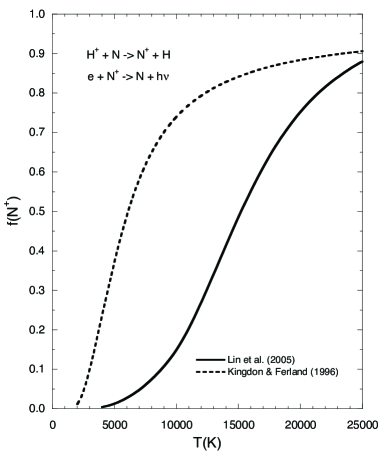
Figure 9: The fractional nitrogen abundance as a function of kinetic temperature due to production by proton charge exchange and destruction by electron recombination. Two charge exchange reaction rate coefficients are plotted; the solid line is from Lin et al. (2005) and the dashed line from Kingdon & Ferland (1996).

4.2 Conclusions

From our analysis of [N ii] emission at the edge of the CMZ near Sgr E we find evidence for dense, hot, highly ionized gas. The association with [C ii] and CO indicates that this dense ionized gas surrounds the PDRs associated with two molecular clouds, one with V_lsr $\sim$ -207 km s^-1 and the other $\sim$ -174 km s^-1. The electron densities, $n$(e) $\sim$ 5 to 21 cm^-3, are considerably higher than those in the WIM of the disk, but consistent with those expected for bright diffuse H ii regions, such as the Carina nebula (Oberst et al. 2011). The electron densities are considerably lower than those suggested by Lazio & Cordes (1998), $n$(e)$\gtrsim$ 10³ cm^-3, if the photoionized layers of clouds are responsible for the scattering of radio waves in the CMZ. However, they are consistent with their other suggestion that the scattering could be due to the interface with a hot ionized medium with $n$(e)$\sim$ 5 - 50 cm^-3 and $T_{k}$(e)$\sim$ 10⁵ – 10⁶ K. We have no information about the kinetic temperature from our observations, and have assumed typical WIM kinetic temperatures $\sim$ 8000K. Furthermore, our results apply to the ionized regions around the molecular cloud and if these are indeed the source of the scattering of radio waves, then they occupy a small filling factor in the CMZ and may not be representative of the electron density in the bulk of the volume.

There are three ways to sustain such a dense highly ionized hydrogen gas with large nitrogen ionization fraction. One is to have a strong EUV radiation field with a flux of order 10⁶ to 10⁷ photons cm^-2 s^-1, another is to have a high enough kinetic temperature for rapid proton charge exchange with nitrogen, and the third is if there is a flux of X-rays sufficient to ionize nitrogen in the diffuse gas. In the case of photoionization and X-ray ionization it is not necessary for the gas to be very hot. For charge exchange, a gas temperature of order 5000 K suffices for the rates from Kingdon & Ferland (1996), but a much higher temperature of order 15000 K is required if the rates calculated by Lin et al. (2005) are correct. We are not able to distinguish which one of these processes dominates the ionization of the gas observed in [N ii], or whether all three contribute. The asymmetry in the [C ii] limb brightening in $b>$0^∘ versus $b<$ 0^∘ may be indicative of an asymmetry in the distribution of ionizing sources. However we lack a complete survey of the Sgr E region in X-rays or EUV from which to draw any firm conclusions.

The edge of the CMZ extends a little farther outwards (smaller $l$) in ionized components than in CO. The ThrUUMS CO map, Figure 6, detects CO at -207 km s^-1 out to $l=$ 358$\aas@@fstack{\circ}$50, whereas the GREAT [C ii] and [N ii] observations show emission out to at least 358$\aas@@fstack{\circ}$45, a difference of 7 pc. Whether the CMZ extends any further cannot be determined as the GREAT observations did not extend to smaller values of $l$, and the HIFI OTF maps, which extend to 358$\aas@@fstack{\circ}$20, are less sensitive than the GREAT [C ii] data and show only a hint of [C ii] at -207 km s^-1 extending to 358$\aas@@fstack{\circ}$35, a distance of 14 pc from the CO edge.

We have also estimated the column density of CO–dark H₂ from [C ii] observations and find an average column density of order 1-2$\times$10²¹ cm^-2. Models of massive molecular clouds (Wolfire et al. 2010; Bolatto et al. 2013) predict such column densities, somewhat independent of the mass of the cloud and of the intensity of the UV field. Observations of [C ii] and CO towards a large ensemble of molecular clouds in the Galactic disk (Langer et al. 2014) are consistent with this model. Thus clouds in the CMZ and disk have similar CO–dark H₂ layers despite differences in UV radiation field and density.

5 Summary

We have explored the ionized gas at the edge of the CMZ near Sgr E, combining deep integrations of spectrally resolved [C ii] (158$\mu$m) and [N ii] (205$\mu$m) at six lines of sight along $b$ = 0^∘ made with the GREAT instrument on SOFIA and HIFI spectrally resolved [C ii] on-the-fly strip maps in $b$ at thirteen longitudes spaced 0$\aas@@fstack{\circ}$05 apart. We detect two distinct features in the [C ii] and [N ii] data, one on the line of sight to a CO molecular cloud at V${}_{lsr}\sim$ -207 km s^-1, associated with Sgr E, and the other at $\sim$ -174 km s^-1 outside the edge of another CO cloud.

We find that the brightest emission in the HIFI strip maps toward the cloud at -207 km s^-1 forms an arc of [C ii] emission above the plane at the edge of the lowest CO contours. It likely represents limb brightened emission in a highly ionized layer outside the molecular cloud. We also detected [N ii] emission at a few positions in this edge, and both [C ii] and [N ii] have very broad lines there with $\Delta V$ of order 25 to 35 km s^-1. The electron density in this region was derived from [N ii] emission and a radiative transfer model, assuming a characteristic size. We find $n$(e) $\sim$ 9 to 21 cm^-3, about three orders of magnitude higher than that characterizing the disk’s warm ionized medium (WIM), much smaller than those of compact H ii regions, but consistent with densities derived from excitation analysis of [N ii] in bright extended H ii regions, such as the Carina nebula (Oberst et al. 2011). The electron densities determined from the [N ii] for the ionized envelope of the cloud associated with Sgr E are lower than those suggested to explain the scattering of radio waves used to derive the average electron density distribution in the CMZ if the scattering comes from the ionized envelope (Lazio & Cordes 1998).

The ionization of such a dense region requires a large flux of EUV radiation, and/or X-ray flux, and/or high enough temperatures to allow rapid charge exchange with protons via the endothermic reaction, H⁺ + N $\rightarrow$ H + N⁺. The presence of abundant N⁺ requires this region to be hot, and the heating could be photoelectron emission from the FUV, EUV, and X-ray radiation fields, dissipation of strong magnetic turbulence, or shock heating of supersonic turbulence. This region has many compact bright H ii sources, indicating that it is an active massive star formation region, and such stars have the capacity to ionize and heat the gas in this region. The CMZ is also a source of diffuse X-rays and discrete X-ray sources that could provide the X-ray flux to ionize the nitrogen (as well as the hydrogen), but it depends on details of the distribution and luminosity of the X-rays. Finally, we estimate that this CO cloud has a layer of CO–dark H₂ with column density $\sim$1-2$\times$10²¹ cm^-2, consistent with theoretical models and observations of clouds in the disk.

We also detect ionized gas at a velocity $\sim$-174 km s^-1 and the lines of sight observed in [C ii] and [N ii] with GREAT have H i but no CO except except at $l=$ 358$\aas@@fstack{\circ}$75 which turns out to be the edge of a molecular cloud mapped in CO (Oka et al. 1998). However this [C ii] emission is weak and the number of [C ii] detections in the HIFI map is insufficient to determine the size of the ionized envelope for this cloud. Therefore to estimate the properties of the envelope we assumed the same thickness as that for the -207 km s^-1 cloud. An analysis of the [N ii] emission using parameters similar to those for the -207 km s^-1 cloud suggests that it too is a hot high density ionized gas with $n$(e)$\sim$ 6 to 10 cm^-3. The physical conditions in this ionized component are likely to be similar to those at the edge of the molecular cloud at $\sim$-207 km s^-1 and have similar heating and ionizing sources. Larger scale maps of spectrally resolved [C ii] and [N ii] will be needed to understand further the role of the ionized gas at the edge of the CMZ. Finally, the CMZ is seen to extend further out in ionized gas from the CO edge by upwards of at least 7 to 14 pc.