Mixed Map Labeling

Abstract

Point feature map labeling is a geometric problem, in which a set of input points must be labeled with a set of disjoint rectangles (the bounding boxes of the label texts). Typically, labeling models either use internal labels, which must touch their feature point, or external (boundary) labels, which are placed on one of the four sides of the input points’ bounding box and which are connected to their feature points by crossing-free leader lines. In this paper we study polynomial-time algorithms for maximizing the number of internal labels in a mixed labeling model that combines internal and external labels. The model requires that all leaders are parallel to a given orientation $\theta\in[0,2\pi)$, whose value influences the geometric properties and hence the running times of our algorithms.

1 Introduction

Annotating features of interest in information graphics with textual labels or icons is an important task in information visualization. One classical application, whose principles easily generalize to the labeling of other illustrations, is map labeling, where labels are mostly placed internally in the map. Common cartographic placement guidelines demand that each label is placed in the immediate neighborhood of its feature and that the association between labels and features is unambiguous, while no two labels may overlap each other [13, 21]. Point feature labeling has been studied extensively in the computational geometry literature, but also in the application areas. It is known that maximizing the number of non-overlapping labels for a given set of input points is NP-hard, even for very restricted labeling models [9, 18]. In terms of labeling algorithms, several approximations, polynomial-time approximation schemes (PTAS), and exact approaches are known [1, 22, 7, 16], as well as many practically effective heuristics, see the bibliography of Wolff and Strijk [23]. If, however, feature points lie too dense in the map or if their labels are relatively large, often only small fractions of the features obtain a label, even in an optimal solution.

An alternative labeling approach using external instead of internal labels is known as boundary labeling in the literature. This labeling style is frequently used when annotating anatomical drawings and technical illustrations, where different and often small parts are identified using labels and descriptive texts outside the actual picture, which are connected to their features using leader lines. While the association between points and external labels is often more difficult to see, the big advantages of boundary labeling are that even dense feature sets can be labeled and that larger labels can be accommodated on the margins of the illustration. Many efficient boundary labeling algorithms are known. They can be classified by the leader shapes that are used and by the sides of the picture’s bounding box that are used for placing the labels [5, 6, 2, 10, 15, 20, 12].

The combination of internal and external labeling models using internal labels where possible and external labels where necessary seems natural and has been proposed as an open problem by Kaufmann [14]; however, only few results are known in such hybrid or mixed settings. In a mixed labeling, the final image will be an overlay of the original map or drawing, a collection of internal text labels, and a collection of leaders leading out of the image. Depending on the application, we may wish to forbid intersections between some or all of these layers. When no additional intersection constraints are imposed, the problem reduces to classical internal map labeling. Under the very natural restriction that leaders cannot intersect internal labels, the internal labels need to be placed carefully, as not every set of disjoint internal labels creates sufficient gaps for routing leaders of the prescribed shape from all remaining feature points to the image boundary. Löffler and Nöllenburg [17] studied a restricted case of hybrid labeling, where a partition of the feature points into points with internal fixed position labels and points with external labels to be connected by one-bend orthogonal leaders is given as input. They presented efficient algorithms and hardness results, depending on three different problem parameters. Bekos et al. [3] studied a mixed labeling model with fixed-position internal labels and external labels on one or two opposite sides of the bounding box, connected by two-bend orthogonal leaders. Their goal is to maximize the number of internally labeled points, while labeling all remaining points externally. Polynomial and quasi-polynomial-time algorithms, as well as an approximation algorithm and an ILP formulation were presented.

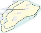
(a) $\theta=\pi$

(b) $\theta=0$

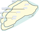
(c) $\theta=\pi/3$

Figure 1: A sample point set with mixed labelings of three different slopes. In (a) five external labels are necessary, whereas (b) and (c) require only four external labels. The slope in (c) yields aesthetically pleasing results.

Contribution

In this paper, we extend the known results on mixed map labeling as follows. We present a mixed labeling model, in which each point is assigned either an axis-aligned fixed-position internal label (e.g., to the top right of the point) or an external label connected with a leader of slope $\theta$, where $\theta\in[0,2\pi)$ is an input parameter defining the unique leader direction for all external labels, measured clockwise from the negative $x$-axis (see Fig. 1). In this model, we present a new dynamic-programming algorithm to maximize the number of internally labeled points for any given slope $\theta$, including the left- and right-sided case ($\theta=0$ or $\theta=\pi$), which was studied by Bekos et al. [3]. While for the right-sided case Bekos et al. provided a faster $O(n\log^{2}n)$-time algorithm, where $n$ is the number of input points, our algorithm improves upon their pseudo-polynomial $O(n^{\log n+3})$-time algorithm for the left-sided case. We solve this problem in $O(n^{3}(\log n+\delta))$ time, where $\delta=\min\{n,1/d_{\min}\}$ is the inverse of the distance $d_{\min}$ of the closest pair of points in $\mathcal{P}$ and expresses the maximum density of $\mathcal{P}$ (Section 2). In the general case it turns out that the set of slopes can be partitioned into twelve intervals, in each of which the geometric properties of the possible leader-label intersections are similar for all slopes. Depending on the particular slope interval, the amount $\iota(n,\delta,\theta)$ of “interference” between sub-problems varies. This significantly affects the algorithm’s performance and leads to running times between $O(n^{3}\log n)$ and $O(n^{3}(\log n+\iota(n,\delta,\theta)))=O(n^{7})$ (Section 3). Moreover, we can use our algorithm to optimize the number of internal labels over all slopes $\theta$ at an increase in running time by a factor of $O(n^{2})$, as is shown in Section 4.1.

Problem Statement

We are given a map (or any other illustration) $\mathcal{M}$, which we model for simplicity as a convex polygon (this is easy to relax to larger classes of well-behaved domains), and a set $\mathcal{P}$ of $n$ points in $\mathcal{M}$ that must be labeled by rectangular labels (the bounding boxes of the label texts). In addition, we are given a leader slope $\theta\in[0,2\pi)$. For simplicity we assume that $\theta$ is none of the slopes defined by two points in $\mathcal{P}$. We discuss in Section 4.4 how to remove this restriction. There are two choices for assigning a label to a point $p\in\mathcal{P}$: either we assign an internal label $\lambda_{p}$ on $\mathcal{M}$ in a one-position model, or an external label outside of $\mathcal{M}$ that is connected to $p$ with a leader $\gamma_{p}$. An internal label $\lambda_{p}$ is a rectangle that is anchored at $p$ by its lower left corner. A leader $\gamma_{p}$ is a line segment of slope $\theta$ inside $\mathcal{M}$; it may bend to the horizontal direction outside of $\mathcal{M}$ in order to connect to its horizontally aligned label, see Fig. 1c. So in this model, the labeling is fixed once the choice for an internal or external label has been made for each point $p\in\mathcal{P}$. For a valid label assignment we require that (i) the internal labels do not overlap each other or the leaders, and that (ii) the leaders themselves do not intersect each other. Figure 1 shows valid mixed labelings for three different slopes.

Given a set of points $P\subseteq\mathcal{P}$, let $\Lambda(P)=\{\lambda_{p}\mid p\in P\}$ denote the set of (candidate) labels corresponding to the points in $P$ and let $\Gamma(P)=\{\gamma_{p}\mid p\in P\}$ denote the set of (candidate) leaders corresponding to the points in $P$. A labeling of $\mathcal{P}$ is a partition of $\mathcal{P}$ into sets $\mathcal{I}$ and $\mathcal{E}$, the points in $\mathcal{I}$ labeled internally, the points in $\mathcal{E}$ labeled externally, such that no two labels in $\Lambda(\mathcal{I})$ intersect, no two leaders in $\Gamma(\mathcal{E})$ intersect, and no label from $\Lambda(\mathcal{I})$ intersects a leader from $\Gamma(\mathcal{E})$.

For ease of presentation we first assume that all labels have the same size, which, without loss of generality, we assume to be $1\times 1$. Hence, an internal label $\lambda_{p}$ is a unit square with its bottom left corner on $p$. This may be a realistic model in some settings (e.g., unit-size icons as labels), but generally not all labels have the same size. We will sketch how to relax this restriction in Section 4.3.

Each leader $\gamma_{p}$ can be split into an inner part (or inner leader), which is a line segment of slope $\theta$ from $p$ to the intersection point with the boundary of $\mathcal{M}$, and an outer part (or outer leader) from the boundary of $\mathcal{M}$ to the actual label. We focus our attention on the inner leaders as they determine how $\mathcal{P}$ is separated into different subinstances. Hence we can basically think of the leaders as half-lines with slope $\theta$. For completeness, we explain a simple method of routing the outer leaders in Section 4.2.

It is well known that in general not all points in $\mathcal{P}$ can be assigned an internal label. The corresponding label number maximization problem is NP-hard [9, 18], even if each label has just one candidate position [17]. If, however, all labels have the same position (e.g., to the top left of the anchor points) and no input point may be covered by any other label, the one-position case can be solved efficiently by first discarding all labels containing an anchor point and then applying a simple greedy algorithm on the resulting staircase patterns [17]. On the other hand, it is also known that any instance can be labeled with external labels using efficient algorithms [5, 4]. Mixed labelings combine both label types and sit between the two extremes of purely internal and purely external labeling [3, 17]. Here we are interested in the internal label number maximization problem, which was first studied for $\theta\in\{0,\pi\}$ by Bekos et al. [3]: Given a map $\mathcal{M}$, a set of points $\mathcal{P}$ in $\mathcal{M}$ and a slope $\theta\in[0,2\pi)$, we wish to find a valid mixed labeling that maximizes the number $|\mathcal{I}|$ of internally labeled points.

2 Leaders from the Left

We start with the case that $\theta=0$, i.e., all leaders are horizontal half-lines leading from the points to the left of $\mathcal{M}$. Our approach for maximizing the number of internal labels is to process the points in $\mathcal{P}$ from right to left and to recursively determine the optimal rightmost unprocessed point $p$ to be assigned an external label. Since no leader may cross any internal label, the leader $\gamma_{p}$ decomposes the current instance left of $p$ into two (almost) independent parts, one above $\gamma_{p}$ and one below. As it turns out, a generic subinstance can be defined by an upper and a lower leader shielding it from the outside and additional information about at most one point outside the subinstance. The problem is then solved using dynamic programming.

2.1 Geometric Properties

Let $p=(p_{x},p_{y})$ be a point in the plane and let $L_{p}=\{q\mid q_{x}<p_{x}\}$ and $R_{p}=\{q\mid q_{x}>p_{x}\}$ denote the half-planes containing all points strictly to the left and to the right of $p$, respectively. Analogously, we define the half-planes $T_{p}$ and $B_{p}$ above and below $p$, respectively. Let $\overline{S(\ell,u)}=T_{\ell}\cap B_{u}$ denote the horizontal slab defined by points $\ell$ and $u$ (with $\ell_{y}<u_{y}$), and let $S(\ell,u)=\overline{S(\ell,u)}\cap L_{\ell}\cap L_{u}$ denote the set of points in this slab that lie to the left of both $\ell$ and $u$, see Fig. 2. We define $P_{\ell,u}$ as the subset of $\mathcal{P}$ in $S(\ell,u)$ including $\ell$ and $u$, i.e., $P_{\ell,u}=\mathcal{P}\cap(S(\ell,u)\cup\{\ell,u\})$. With some abuse of notation we will sometimes also use $L_{p}$, $R_{p}$, $T_{p}$, and $B_{p}$ to mean the subset of $\mathcal{P}$ that lies in the respective half-plane rather than the entire half-plane.

(a)

(b)

Figure 2: The slab $\overline{S(\ell,u)}$ in yellow, the region $S(\ell,u)$ and its points from $\mathcal{P}$ in purple, and the region $E(\ell)$ in blue.

Recall that $\delta=\min\{n,1/d_{\min}\}$ is a parameter that captures the maximum density of $\mathcal{P}$ as the inverse of the smallest distance $d_{\min}$ between any two points in $\mathcal{P}$. We can use $\delta$ to bound the number of points in a unit square that may be labeled internally.

Lemma 1.

At most $O(\delta)$ points in any unit square have a label $\lambda$ that does not contain another point in $\mathcal{P}$.

Proof.

Let $E$ be a unit square and let $E_{\mathcal{P}}=E\cap\mathcal{P}$ be the input points in $E$. Since the label $\lambda_{p}$ of every point $p\in E_{\mathcal{P}}$ is a unit square anchored by its lower left corner at $p$, no other point $q\in\mathcal{P}$ may lie to the top-right of $p$—otherwise $p$ must be labeled externally. Hence any set of points in $E_{\mathcal{P}}$ whose labels do not contain another point of $\mathcal{P}$ must form a sequence $p^{(1)},p^{(2)},\dots,p^{(k)}$ such that $p^{(i)}_{x}<p^{(j)}_{x}$ and $p^{(i)}_{y}>p^{(j)}_{y}$ for any $i<j$. Since the minimum distance of any two points is $d_{\min}$ we immediately obtain that $E_{\mathcal{P}}$ contains at most $O(\delta)$ points that can be labeled internally. ∎

Next, we characterize which leaders or labels outside of $\overline{S(\ell,u)}$ can interfere with a potential labeling of $P_{\ell,u}$ assuming $\ell$ and $u$ are labeled externally.

Lemma 2.

Let $\ell,u\in\mathcal{P}$, let $(\mathcal{I}^{\prime},\mathcal{E}^{\prime})$, with $\ell,u\in\mathcal{E}^{\prime}$ be a labeling of $P_{\ell,u}$. There is no point in $T_{u}\cup B_{\ell}$ whose leader intersects a label from $\Lambda(\mathcal{I}^{\prime})$ and there is no point in $T_{u}$ whose label intersects a label from $\Lambda(\mathcal{I}^{\prime})$.

Proof.

In any labeling of $P_{\ell,u}$ there are no intersections between labels and leaders. In particular, no label $\lambda_{p}$ for $p\in\mathcal{I}^{\prime}$ intersects $\gamma_{\ell}$ or $\gamma_{u}$. It follows that all labels for $\mathcal{I}^{\prime}$ lie inside the slab $\overline{S(\ell,u)}$. By definition, all leaders for $\mathcal{E}^{\prime}$ also lie inside $\overline{S(\ell,u)}$. Since leaders of points in $T_{u}\cup B_{\ell}$ do not intersect $\overline{S(\ell,u)}$, no such leader can intersect a label from $\mathcal{I}^{\prime}$. Moreover, all labels are anchored by their bottom left corner, and hence all labels of points in $T_{u}$ lie above $u$ and do not intersect $\overline{S(\ell,u)}$. Thus, no label for a point in $T_{u}$ can intersect a label in $\Lambda(\mathcal{I}^{\prime})$. ∎

It is not true, however, that labels for points in $B_{\ell}$ cannot intersect labels for $P_{\ell,u}$. Still, the influence of $B_{\ell}$ is very limited as the next lemma shows. Let $E(\ell)$ denote the open unit square with top-left corner $\ell$, i.e., $E(\ell)=R_{\ell}\cap B_{\ell}\cap L_{r}\cap T_{b}$, where $r=(\ell_{x}+1,\ell_{y})$ and $b=(\ell_{x},\ell_{y}-1)$. See Fig. 2b.

Lemma 3.

Let $\ell,u\in\mathcal{P}$, let $(\mathcal{I}^{\prime},\mathcal{E}^{\prime})$, with $\ell,u\in\mathcal{E}^{\prime}$ be a labeling of $P_{\ell,u}$, and let $(\mathcal{I}^{\prime\prime},\mathcal{E}^{\prime\prime})$ denote a labeling of $\mathcal{P}\cap B_{\ell}\cup\{\ell\}$ with $\ell\in\mathcal{E}^{\prime\prime}$. There is at most one point $p\in\mathcal{I}^{\prime\prime}$ whose label may intersect a label of $\mathcal{I}^{\prime}$, and $p\in E(\ell)$.

Proof.

Since $\ell\in\mathcal{E}^{\prime}\cap\mathcal{E}^{\prime\prime}$ we know that no label in $\Lambda(\mathcal{I}^{\prime})$ or $\Lambda(\mathcal{I}^{\prime\prime})$ intersects $\gamma_{\ell}$. Thus $\gamma_{\ell}$ serves as a separation line between the labels $\Lambda(\mathcal{I}^{\prime})$ and $\Lambda(\mathcal{I}^{\prime\prime})$. Let $\mathcal{P}^{\prime\prime}\subseteq\mathcal{I}^{\prime\prime}$ denote the set of points whose labels intersect a label of $\mathcal{I}^{\prime}$, and let $\Lambda^{\prime\prime}=\Lambda(\mathcal{P}^{\prime\prime})$ denote the corresponding set of labels. We first argue that $\mathcal{P}^{\prime\prime}\subseteq E(\ell)$. Then we argue that $\mathcal{P}^{\prime\prime}$ can contain at most one point.

The labels in $\Lambda^{\prime\prime}$ do not intersect $\gamma_{\ell}$, hence they lie strictly right of $\ell$. Thus, $\mathcal{P}^{\prime\prime}\subseteq R_{\ell}$. All points in $\mathcal{I}^{\prime}$ lie to the left of $\ell$, and their labels have width one. All labels in $\Lambda^{\prime\prime}$ intersect such a label, thus all points in $\mathcal{P}^{\prime\prime}$ must lie in $L_{r}$, where $r=(\ell_{x}+1,\ell_{y})$. All labels in $\Lambda^{\prime\prime}$ intersect a label from a point in $\mathcal{I}^{\prime}$. Thus, all labels in $\Lambda^{\prime\prime}$ intersect the horizontal line containing $\gamma_{\ell}$. Since all labels have height one, it follows that all points in $\mathcal{P}^{\prime\prime}$ lie in $T_{b}$, where $b=(\ell_{x},\ell_{y}-1)$. By definition the points in $\mathcal{P}^{\prime\prime}$ lie in $B_{\ell}$. So we have $\mathcal{P}^{\prime\prime}\subseteq R_{\ell}\cap L_{r}\cap T_{b}\cap B_{\ell}=E(\ell)$.

The labels in $\Lambda^{\prime\prime}$ are pairwise disjoint and all intersect the top side $s$ of $E(\ell)$. Since the length of $s$ is smaller than one, each label in $\Lambda^{\prime\prime}$ has width exactly one, and all labels lie in $R_{\ell}$ it follows that there can be at most one label in $\Lambda^{\prime\prime}$. Thus, there is also at most one point in $\mathcal{P}^{\prime\prime}$. ∎

From Lemma 2 and Lemma 3 it follows that if $\ell$ and $u$ are labeled externally, there is at most one point $r$ below $\ell$ that can influence the labeling of the points in $S(\ell,u)$.

2.2 Computing an Optimal Labeling

We define $\Phi(\ell,u,r)$, with $\ell,u\in\mathcal{P}$, and $r\in E(\ell)\cup\{\bot\}$ as the maximum number of points in $S(\ell,u)$ that can be labeled internally, given that

1. the points $\ell$ and $u$ are labeled externally,

2. all remaining points in $\overline{S(\ell,u)}\setminus S(\ell,u)$ have been labeled internally, and

3. point $r$ is labeled internally. If $r=\bot$ then no point in $E(\ell)$ is labeled internally.

See Fig. 3(a) for an illustration. Furthermore, given $\ell$, $r$, and a point $p\in T_{\ell}$ we define $\varrho(p,\ell,r)$ to be the topmost point in $E(p)\cap(T_{\ell}\cup\{r\})$ if such a point exists. Otherwise we define $\varrho(p,\ell,r)=\bot$.

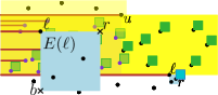
(a)

(b)

Figure 3: (a) $\Phi(\ell,u,r)$ expresses the maximum number of points in $S(\ell,u)$ (purple), that can be labeled internally in the depicted situation. (b) The rightmost point $p$ that is labeled with an external label decomposes the problem into two subproblems (the orange and blue points).

Lemma 4.

For any $\ell,u\in\mathcal{P}$, and $r\in E(\ell)\cup\{\bot\}$, we have that $\Phi(\ell,u,r)=|S(\ell,u)|$, or $\Phi(\ell,u,r)=|R_{p}\cap S(\ell,u)|+\Phi(\ell,p,r)+\Phi(p,u,r^{\prime})$, where $p$ is the rightmost point in $S(\ell,u)$ with an external label and $r^{\prime}=\varrho(p,\ell,r)$.

Proof.

Let $(\mathcal{I}^{*},\mathcal{E}^{*})$ be an optimal labeling of $S(\ell,u)$ that satisfies the constraints (i)–(iii) on $\Phi(\ell,u,r)$, i.e., $\Phi(\ell,u,r)=|\mathcal{I}^{*}|$. In case $\mathcal{E}^{*}=\emptyset$, we have $\Phi(\ell,u,r)=|S(\ell,u)|$ and the lemma trivially holds. Otherwise, there must be a rightmost point $p\in\mathcal{E}^{*}$ with an external label. Consider the partition of $\mathcal{I}^{*}$ at point $p$ into the lower left part $B^{*}=B_{p}\cap L_{p}\cap\mathcal{I}^{*}$, the upper left part $T^{*}=T_{p}\cap L_{p}\cap\mathcal{I}^{*}$, and the right part $R^{*}=R_{p}\cap\mathcal{I}^{*}$, see Fig. 3b. We show that $|R^{*}|=|R_{p}\cap S(\ell,u)|$, $|B^{*}|=\Phi(\ell,p,r)$, and $|T^{*}|=\Phi(p,u,r^{\prime})$, which proves the lemma.

Since $p$ is the rightmost point with an external label it follows that all points in $S(\ell,u)$ right of $p$ are labeled internally. Hence, $R^{*}=R_{p}\cap S(\ell,u)$.

Next, we observe that $\mathcal{L}_{B}=(B^{*},S(\ell,p)\setminus B^{*})$ as a sub-labeling of $(\mathcal{I}^{*},\mathcal{E}^{*})$ forms a valid labeling of $S(\ell,p)$, so by Lemma 3 there is at most one point $\hat{r}$ below $\ell$ that can influence the labeling of $S(\ell,p)$. This point $\hat{r}$, if it exists, lies in $E(\ell)$. By constraint (iii) point $r$ lies in $E(\ell)$ or $r=\bot$ and no point in $E(\ell)$ is labeled internally, and thus $r$ can be the only point in $E(\ell)$ labeled internally, i.e., $\hat{r}=r$. So, we have that (i) $\ell$ and $p$ are labeled externally, (ii) all points in $\overline{S(\ell,p)}\setminus S(\ell,p)$ are labeled internally, and (iii) point $r$ is the only internally labeled point in $E(\ell)$. Thus the definition of $\Phi$ applies and we obtain $|B^{*}|\leq\Phi(\ell,p,r)$.

Lemmas 2 and 3 together imply that any labeling of $S(\ell,p)$ is independent from any labeling of $S(p,u)$. Thus, it follows that $\mathcal{L}_{B}$ is an optimal labeling of $S(\ell,p)$ (given the constraints), since otherwise $(\mathcal{I}^{*},\mathcal{E}^{*})$ could also be improved. Thus $|B^{*}|\geq\Phi(\ell,p,r)$ and we obtain $|B^{*}|=\Phi(\ell,p,r)$.

Finally, we consider the upper left part $\mathcal{T}^{*}$. By Lemma 3 there is at most one point $r^{\prime}$ in $B_{p}$ with an internal label that can influence the labeling of $S(p,u)$ and we have $r^{\prime}\in E(p)$. We need to show that $r^{\prime}=\varrho(p,\ell,r)$. Then the rest of the argument is analogous to the argument for $B^{*}$.

We claim that $r^{\prime}$ is the topmost point in $E(p)\cap(T_{\ell}\cup\{r\})$. Assume that $r^{\prime}\not\in T_{\ell}$, which means $r^{\prime}\in B_{\ell}$. We know that $\gamma_{\ell}$ does not intersect $\lambda_{r^{\prime}}$ and hence $r^{\prime}\in R_{\ell}$. This means that $r^{\prime}\in E(p)\cap B_{\ell}\cap R_{\ell}=:X$ and since $p$ lies to the top-left of $\ell$ we have $X\subseteq E(\ell)$. By definition $r$ is the only point with an internal label in $E(\ell)$ and hence $r^{\prime}=r$. So if $r^{\prime}\neq r$ we have $r^{\prime}\in E(p)\cap T_{\ell}$. Now assume that $r^{\prime}\neq\varrho(p,\ell,r)$. Then there is another point $q\in E(p)\cap T_{\ell}$ above $r^{\prime}$. This point $q$ must be labeled externally since no two points in $E(p)$ can be labeled internally. This is a contradiction since by definition $p$ is the rightmost externally labeled point in $S(\ell,u)$ and by constraint (ii) all points in $\overline{S(\ell,u)}\setminus S(\ell,u)$ are labeled internally. So indeed $r^{\prime}=\varrho(p,\ell,r)$ and the same arguments as for $B^{*}$ can be used to obtain $|T^{*}|=\Phi(p,u,r^{\prime})$. ∎

Let $\ell$, $u\in\mathcal{P}$, and $p\in S(\ell,u)$. We observe that $|S(\ell,p)|$ and $|S(p,u)|$ are strictly smaller than $|S(\ell,u)|$. Thus, Lemma 4 gives us a proper recursive definition for $\Phi$:

$$\Phi(\ell,u,r)=\max\big{\{} \Psi(S(\ell,u)),$$

$$\max_{p\in S(\ell,u)}\left\{\Psi(R_{p}\cap S(\ell,u))+\Phi(\ell,p,r)+\Phi(p,u,\varrho(p,\ell,r))\right\}\big{\}},$$

where

$$\Psi(P)=\begin{cases}|P|&\parbox{303.53267pt}{if all labels in $\Lambda(P\cup\{r\}\cup(\overline{S(\ell,u)}\setminus S(\ell,u)))$ are pairwise disjoint, and their intersection with $\gamma_{\ell}$ and $\gamma_{u}$ is empty,}\\ -\infty&\text{otherwise}.\end{cases}$$

We can now express the maximum number of points in $\mathcal{P}$ that can be labeled internally using $\Phi$. We add two dummy points to $\mathcal{P}$ that we assume are labeled externally: a point $p_{\infty}$ that lies sufficiently far above and to the right of all points in $\mathcal{P}$, and a point $p_{-\infty}$ below and to the right of all points in $\mathcal{P}$. The maximum number of points labeled internally is then $\Phi(p_{-\infty},p_{\infty},\bot)$.

We use dynamic programming to compute $\Phi(\ell,u,r)$ for all $\ell,u\in\mathcal{P}\cup\{p_{\infty},p_{-\infty}\}$ with $\ell_{y}<u_{y}$ and $r\in E(\ell)\cup\{\bot\}$. By finding the maximum in a set of linear size, each value $\Phi(\ell,u,r)$ can be computed in $O(n)$ time, given that the values $\Phi(\ell^{\prime},u^{\prime},r^{\prime})$ for all subproblems have already been computed and stored in a table and the relevant values for the functions $\varrho$ and $f$ have been precomputed. There are $O(n)$ choices for each of $\ell$ and $u$; further there are $O(\delta)$ choices for the point $r$ given $\ell$ since $r$ is labeled internally and we know from Lemma 1 that there are at most $O(\delta)$ points in $E(\ell)$ as candidates for an internal label. This results in an $O(n^{3}\delta)$ time and $O(n^{2}\delta)$ space dynamic-programming algorithm. We show next that the preprocessing of $\varrho$ and $f$ can be done in $O(n^{3}\log n)$ time.

To compute $\Phi(\ell,u,r)$ we actually have to compute $\varrho(p,\ell,r)$ and $\Psi^{\prime}(p,r):=\Psi(R_{p}\cap S(\ell,u))$ for all points $p\in S(\ell,u)$. We can preprocess all points in $\mathcal{P}$ in $O(n\log n)$ time, such that we can compute each $\varrho(p,\ell,r)$ in $O(1)$ time as follows. First, we compute and store for each point $p\in\mathcal{P}$ the topmost point $q_{p}\in\mathcal{P}$ in $E(p)$. This requires $n$ standard priority range queries that take $O(n\log n)$ time in total using priority range trees with fractional cascading [8, Chapter 5]. To compute $\varrho(p,\ell,r)$ we then check if $q_{p}$ lies above $\ell$. If it does, we have $\varrho(p,\ell,r)=q_{p}$. Otherwise, the only candidate point for $\varrho(p,\ell,r)$ is $r$ and we can check in $O(1)$ time if $r$ lies in $E(p)$. This takes $O(1)$ time for each triple $(p,\ell,r)$ and $O(n^{2}\delta)$ time in total.

Next, we fix $\ell$ and $u$, and compute a representation of $\Psi^{\prime}$ in $O(n\log n)$ time, such that for each $p\in S(\ell,u)$ and $r\in E(\ell)\cup\{\bot\}$ we can obtain $\Psi^{\prime}(p,r)$ in constant time.

We start by computing the values $\Psi^{\prime}(p,\bot)$, for all $p$. We sweep a vertical line from right to left. That is, we sort all points in $\overline{S(\ell,u)}$ by decreasing $x$-coordinate, and process the points in that order. The status structure of the sweep line contains the number of points $N$ in $S(\ell,u)$ right of the sweep line, and a (semi-)dynamic data structure $\mathcal{T}$, which stores the labels from the points right of the sweep line, and can report all labels intersected by an (axis-parallel) rectangular query window. All labels are unit squares, so $\lambda_{r}$ intersects a label $\lambda_{q}$ if and only if $\lambda_{r}$ contains a corner point of $\lambda_{q}$. Furthermore, we only ever insert new labels (points) into $\mathcal{T}$, thus it suffices if $\mathcal{T}$ supports only insert and query operations. It follows that we can implement $\mathcal{T}$ using a semi-dynamic range tree using dynamic fractional cascading [19]. In this data structure insertions and queries take $O(\log n)$ time.

When we encounter a new point $p$, $p\not\in\{\ell,u\}$ we test if the label of $p$ intersects any of the labels encountered so far. We can test this using a range query in the tree $\mathcal{T}$. If $p\in S(\ell,u)$ we also explicitly test if $\lambda_{p}$ intersects $\gamma_{\ell}$ or $\gamma_{u}$. If there are no points in the query range $\lambda_{p}$, and $\lambda_{p}$ does not intersect $\gamma_{\ell}$ or $\gamma_{u}$ we report $\Psi^{\prime}(p,\bot)=N$, increment $N$ (if applicable), and insert the corner points of $\lambda_{p}$ into $\mathcal{T}$. If the query range $\lambda_{p}$ is not empty, it follows that $\Psi^{\prime}(p^{\prime},\bot)=-\infty$, for $p^{\prime}=p$ as well as for any point to the left of $p$. Hence, we report that and stop the sweep. Our algorithm runs in $O(n\log n)$ time: sorting all points takes $O(n\log n)$ time, and handling each of the $O(n)$ events takes $O(\log n)$ time.

Now consider a point $r\in E(\ell)$. We observe that for all points $p$ right of $r$, we have that $\Psi^{\prime}(p,r)=\Psi^{\prime}(p,\bot)=0$ since $r$ is right of all points in $S(\ell,u)$. Consider the points left of $r$ ordered by decreasing $x$-coordinate. There are two options, depending on whether or not $\lambda_{r}$ intersects the label $\lambda_{p}$ of the current point $p$. If $\lambda_{r}$ intersects $\lambda_{p}$, we have $\Psi^{\prime}(p,r)=-\infty$ as well as $\Psi^{\prime}(p^{\prime},r)=-\infty$ for all points $p^{\prime}$ left of $p$. If $\lambda_{r}$ does not intersect $\lambda_{p}$ we still have $\Psi^{\prime}(p,r)=\Psi^{\prime}(p,\bot)$. We can test if $\lambda_{r}$ intersects any other label using a range priority query with $\lambda_{r}$ in (the final version of) the range tree $\mathcal{T}$. We need $O(\delta)$ such queries, which take $O(\log n)$ time each. This gives a total running time of $O(n\log n)$. We then conclude:

The above algorithm can also be used when the leaders have a slope $\theta\neq 0$. However, the data structure $\mathcal{T}$ that we use is fairly complicated. In this specific case where $\theta=0$, we can also use a much easier data structure, and still get a total running time of $O(n\log n)$. Instead of using the semi-dynamic range tree as status structure, we use a simple balanced binary search tree that stores (the end-points of) a set of vertical forbidden intervals. When we encounter a new point $p$, we check if $p_{y}$ lies in a forbidden interval. If this is the case then $\lambda_{p}$ intersects another label. Otherwise we can label $p$ internally. This set of forbidden intervals is easily maintained in $O(\log n)$ time.

We use this algorithm for every pair $(\ell,u)$. Hence, after a total of $O(n^{3}\log n)$ preprocessing time, we can answer $\Psi^{\prime}(p,r)$ queries for any $p$ and $r$ in constant time. This yields the following result, which improves the previously best known pseudo-polynomial $O(n^{\log n+3})$-time algorithm of Bekos et al. [3] for the left-sided case $\theta=0$.

Theorem 5.

Given a set $\mathcal{P}$ of $n$ points, we can compute a labeling of $\mathcal{P}$ that maximizes the number of internal labels for $\theta=0$ in $O(n^{3}\log n+n^{3}\delta)$ time and $O(n^{2}\delta)$ space, where $\delta=\min\{n,1/d_{\min}\}$ for the minimum distance $d_{\min}$ in $\mathcal{P}$.

3 Other Leader Directions

For other leader slopes $\theta\neq 0$ we use a similar approach as before. We consider a sub-problem $S(\ell,u)$ defined by two externally labeled points $\ell$ and $u$. We again find the “rightmost” point in the slab labeled externally. This gives us two sub-problems, which we solve recursively using dynamic programming. However, there are four complications:

• The region $E(\ell)$ containing the points “below” the slab $\overline{S(\ell,u)}$ that can influence the labeling of $S(\ell,u)$ is no longer a unit square. Depending on the orientation, it can contain more than one point with an internal label. See Fig. 4(a).

• In addition to the region $E(\ell)$, which contains points that can interfere with a subproblem from below, we now also need to consider a second region, which we call $F(u)$, containing points whose labels can interfere with a subproblem from above. See Fig. 4(b).

• The labels of points in $S(\ell,u)$ are no longer fully contained in the slab $\overline{S(\ell,u)}$. Hence, we have to check that they do not intersect with leaders of points outside $\overline{S(\ell,u)}$. See Fig. 4(b).

• The regions $E(p)$ and $F(p)$ are no longer strictly to “the right” of $p$. Hence, for some sub-problems we may have already decided (by definition of the sub-problem) that a point $q\in E(p)$ that lies “left” of $p$ is labeled internally. Hence, we can no longer choose $q$ to be the rightmost point in $S(\ell,p)$ to be labeled externally.

Figure 4: (a) There may be more than one point “below” $\ell$ with an internal label if the leaders arrive from the bottom left. (b) For other directions there is also a region $F(u)$ “above” the subproblem that can influence the labeling of $S(\ell,u)$.

We start by explicitly finding the points in $\mathcal{P}$ whose internal labels contain other points. We are forced to label these points externally. It is easy to find those points in $O(n^{2})$ time in total. Let $\mathcal{P}_{X}$ denote this set of points. Additionally, we spend $O(n^{2})$ time to mark each point if its label intersects $\Gamma(\mathcal{P}_{X})$. Hence, for each point we can determine in constant time if it intersects $\Gamma(\mathcal{P}_{X})$. For ease of notation we will write $\mathcal{P}$ to mean the set $\mathcal{P}\setminus\mathcal{P}_{X}$ in the remainder of this section.

Let $\theta$ be the given orientation for the leaders. Consider conceptually rotating the coordinate system such that orientation $\theta$ corresponds to the negative $x$-axis as in the previous section, and let $\tilde{B_{p}},\tilde{T_{p}},\tilde{L_{p}},$ and $\tilde{R_{p}}$ denote the points in $\mathcal{P}$ in the bottom, top, left, and right half-planes bounded by $p$ with respect to this coordinate system. Analogously, we define $\overline{S(\ell,u)}=\tilde{T_{\ell}}\cap\tilde{B_{u}}$, and $S(\ell,u)=\overline{S(\ell,u)}\cap\tilde{L_{\ell}}\cap\tilde{L_{u}}$.

Our goal is again to bound the number of different labelings of the points in $\tilde{B_{\ell}}$ and $\tilde{T_{u}}$ that can influence the labeling of $S(\ell,u)$. We will show that whether a labeling of $\tilde{B_{\ell}}$ influences the labeling of $S(\ell,u)$ depends only on a small subset of the points in $\tilde{B_{\ell}}$. We refer to a labeling of $\tilde{B_{\ell}}$ restricted to those points as a configuration of $\tilde{B_{\ell}}$. The same holds for the points in $\tilde{T_{u}}$.

3.1 Bounding the number of Configurations

We start by bounding the number of configurations of $\tilde{B_{\ell}}$. Let $E(\ell)$ denote the bottom influence region of $\ell$. That is, the points in $\tilde{B_{\ell}}$ “below” the slab $\overline{S(\ell,u)}$ whose label can intersect a label of a point in $S(\ell,u)$. Fig. 5 shows the regions $E(\ell)$ for various orientations of the leaders.

Similarly, we can define a region $E^{\prime}(\ell)\subset\tilde{B_{\ell}}$ such that the leaders of points in $E^{\prime}(\ell)$ can intersect a label of a point in $S(\ell,u)$.

Lemma 6.

For a subproblem $S(\ell,u)$ the size of the bottom influence region $E(\ell)$ is at most $1\times e(\theta)$ or $e(\theta)\times 1$, where

$\displaystyle e(\theta)\leq\begin{cases}1&\text{if }\theta=0\\ 2&\text{if }\theta\in(0,\pi/4)\\ 1&\text{if }\theta\in[\pi/4,\pi/2)\\ 0&\text{if }\theta=\pi/2\\ 1&\text{if }\theta\in(\pi/2,3\pi/4)\\ \end{cases}$

$\displaystyle e(\theta)\leq\begin{cases}0&\text{if }\theta\in[3\pi/4,5\pi/4]\\ 1&\text{if }\theta\in(5\pi/4,3\pi/2)\\ 0&\text{if }\theta=3\pi/2\\ 3&\text{if }\theta\in(3\pi/2,7\pi/4)\\ 2&\text{if }\theta\in[7\pi/4,2\pi).\\ \end{cases}$

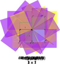
Figure 5: The region $E(\ell)$ (blue) with respect to sub-problem $S(\ell,u)$ (purple), depending on the orientation $\theta$ of the leaders. For each orientation we give an upper bound on the size of $E(\ell)$.

Proof.

We prove this by case distinction on $\theta$.

fnum@@desciitemcase $\theta=0$.

See Lemma 3.

fnum@@desciitemcase $\theta\in(0,\pi/4)$.

All labels in $\Lambda(S(\ell,u))$ lie in $T_{\ell}$ and in $\tilde{L_{r}}$, where $r=(\ell_{x}+1,\ell_{y})$. It follows that $E(\ell)\subseteq T_{\ell^{\prime}}\cap\tilde{L_{r^{\prime}}}$, where $\ell^{\prime}=(\ell_{x},\ell_{y}-1)$ and $r^{\prime}=(r_{x},r_{y}-1)$. Furthermore, it is easy to see that $E(\ell)\subset R_{\ell}$, and that $E(\ell)\subset\tilde{B_{\ell}}$. Hence, $E(\ell)\subset T_{\ell^{\prime}}\cap R_{\ell}\cap\tilde{L_{r^{\prime}}}\cap\tilde{B_{\ell}}$.

Since the leaders are sloped downwards it follows that the height of $E(\ell)$ is at most one. The maximum width of $E(\ell)$ is realized by $\ell$ and the intersection point $p$ of the lines bounding $\tilde{B_{\ell}}$ and $\tilde{L_{r^{\prime}}}$. Using that $\theta\in(0,\pi/4)$ basic trigonometry shows that the width is at most two.

fnum@@desciitemcase $\theta\in[\pi/4,\pi/2)$.

Similar to the previous case. However, now the width is determined by the intersection between $T_{\ell^{\prime}}$ and $\tilde{B_{\ell}}$. From basic trigonometry it then follows that the width is at most one.

fnum@@desciitemcase $\theta=\pi/2$.

For labels from $E(\ell)$ to intersect $\Lambda(S(\ell,u))$ we need $E(\ell)\subset T_{\ell^{\prime}}$, where $\ell^{\prime}=(\ell_{x},\ell_{y}-1)$. However, to avoid intersecting $\gamma_{\ell}$ we need $E(\ell)\subset B_{\ell^{\prime}}$. It follows that $E(\ell)=\emptyset$.

fnum@@desciitemcase $\theta\in(\pi/2,3\pi/4)$.

Using similar arguments as before it follows that $E(\ell)\subset B_{\ell^{\prime}}\cap\tilde{L_{\ell^{\prime}}}\cap\tilde{B_{\ell}}\cap L_{\ell}\cap R_{\ell^{\prime}}$, where $\ell^{\prime}=(\ell_{x}-1,\ell_{y}-1)$. Since $E(\ell)\subset L_{\ell}\cap R_{\ell^{\prime}}$ the width is at most one. Basic trigonometry again shows that the height is at most one.

fnum@@desciitemcase $\theta\in{[3\pi/4,5\pi/4]}$.

For the sub-case $\theta\in[3\pi/4,\pi)$ the lines bounding $\tilde{L_{\ell}}$ and $R_{\ell^{\prime}}$, with $\ell^{\prime}=(\ell_{x}-1,\ell_{y}-1)$ intersect below the line containing $\gamma_{\ell}$. We then obtain $E(\ell)\subset R_{\ell^{\prime}}\cap B_{\ell^{\prime}}\cap\tilde{B_{\ell}}=\emptyset$. In the remaining sub-case $\theta\in[\pi,5\pi/4]$ the regions $\Lambda(S(\ell,u))$ and $\Lambda(\tilde{B_{\ell}})$ are disjoint. It follows that $E(\ell)$ is empty.

fnum@@desciitemcase $\theta\in{(5\pi/4,3\pi/2)}$.

Point $\ell$ is now the point with the maximum $y$-coordinate. It then follows that all labels of $S(\ell,u)$ lie in $B_{\ell^{\prime}}$, where $\ell^{\prime}=(\ell_{x},\ell_{y}+1)$. Hence, we also get $E(\ell)\subset B_{\ell^{\prime}}$. The labels of $S(\ell,u)$ do not intersect $\gamma_{\ell}$, hence they are contained in $L_{\ell}\cup\tilde{T_{\ell}}$. We then have $E(\ell)\subset\tilde{B_{\ell}}\cap(L_{\ell}\cup\tilde{T_{\ell}})=\tilde{B_{\ell}}\cap L_{\ell}$. Since $\theta\in(3\pi/4,3\pi/2)$ it now follows that the height and width are both at most one.

fnum@@desciitemcase $\theta=3\pi/2$.

All labels from $S(\ell,u)$ lie in $L_{\ell}$, all labels from $\tilde{B_{\ell}}=R_{\ell}$ lie in $R_{\ell}$. Hence, $E(\ell)=\emptyset$.

fnum@@desciitemcase $\theta\in(3\pi/2,7\pi/4)$.

It is again easy to show that $E(\ell)\subset R_{\ell}\cap L_{r}$, where $r=(\ell_{x}+1,\ell_{y}+1)$, and thus has width (at most) one. All labels from points in $S(\ell,u)$ have width and height one, and are thus contained in $\tilde{L_{r}}$. Furthermore, they do not intersect $\gamma_{\ell}$, from which we obtain that they are contained in $\tilde{T_{\ell}}\cup T_{\ell}$. From the former we get that $E(\ell)\subset\tilde{L_{r}}$. From the latter we get that $E(\ell)\subset\tilde{T_{\ell^{\prime}}}\cup T_{\ell^{\prime}}$, where $\ell^{\prime}=(\ell_{x},\ell_{y}-1)$. Hence, we obtain $E(\ell)\subset R_{\ell}\cap L_{r}\cap\tilde{L_{r}}\cap(\tilde{T_{\ell^{\prime}}}\cup T_{\ell^{\prime}})\cap\tilde{B_{\ell}}$.

Since $\theta\in(3\pi/2,7\pi/4)$ the height of $E(\ell)$ is determined by $\ell^{\prime}$ and the intersection point $p$ between $\tilde{B_{\ell}}$ and $\tilde{L_{r}}$. Trigonometry now shows that the height is at most three.

fnum@@desciitemcase $\theta\in[7\pi/4,2\pi)$.

Similar to the previous case we get a width of at most one. The height is now determined by $\ell^{\prime}$ and the intersection of $\tilde{B_{\ell}}$ and $R_{r}$. Since $\theta\in[7\pi/4,2\pi)$ the height is at most two.

∎

Corollary 7.

There can be at most $e(\theta)$ points in $E(\ell)$ labeled internally such that their labels are disjoint.

Next, we turn our attention to the points in $E^{\prime}(\ell)$ whose leader can intersect a label of a point in $S(\ell,u)$. A leader of a point in $\tilde{B_{\ell}}$, and thus in $E^{\prime}(\ell)$, can intersect a label of $S(\ell,u)$ only if the labels intersect $\tilde{B_{\ell}}$. This happens only if $\theta\in(5\pi/4,3\pi/2)$ or $\theta\in(3\pi/2,2\pi)$. See Fig. 5. In the former case we thus have $E^{\prime}(\ell)=\tilde{B_{\ell}}\cap\tilde{T_{\ell^{\prime}}}\cap L_{\ell}$, where $\ell^{\prime}=(\ell_{x},\ell_{y}+1-\tan(\theta-5\pi/4))$, and in the latter case we have $E^{\prime}(\ell)=\tilde{B_{\ell}}\cap\tilde{T_{z}}\cap T_{z}$, where $z=(\ell_{x}+1,\ell_{y})$. See Fig. 6.

We now note that if we label the set $Q\subseteq E(\ell)$ internally, then all other points in $E(\ell)$ are labeled externally. Hence, if the leaders of the remaining points (e.g. those in $E(\ell)\setminus Q$) intersect with labels of points in $S(\ell,u)$, this is already captured by the configuration involving $Q$. Therefore, the points in $E(\ell)\setminus Q$ themselves do not define new configurations. Similarly, the points in $\mathcal{P}_{X}$ do not define any new configurations.

The points in $E^{\prime}(\ell)$ that lie outside of $E(\ell)$ can still be labeled both internally or externally. Let $E^{\prime\prime}(\ell)=E^{\prime}(\ell)\setminus E(\ell)$ denote the region containing these points. We now observe:

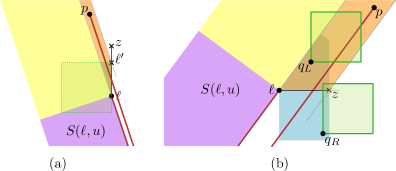
Figure 6: The region $E^{\prime}(\ell)$ (in pink) for the cases $\theta\in(5\pi/4,3\pi/2)$ (a) and $\theta\in(3\pi/2,2\pi)$ (b). In both cases the leader $\gamma_{p}$ of a point $p\in E^{\prime\prime}(\ell)$ intersects the line segment $\overline{\ell{}z}$ and thus subdivides $E(\ell)$ into a left region $L$ and a right region $R$.

Lemma 8.

Let $Q$ be the set of points in $E(\ell)$ labeled internally, and let $p\in E^{\prime\prime}(\ell)$ be labeled externally. For all points $q\in Q$ we have: $q$ intersects the leader $\gamma_{p}$, or if there is a label $\lambda_{a}$, $a\in S(\ell,u)$, that intersects $\lambda_{q}$, then it also intersects the leader $\gamma_{p}$.

Proof.

It is easy to see that any leader $\gamma_{p}$ intersects the line segment $\overline{\ell{}z}$, with $z=(\ell_{x},\ell_{y}+1)$ if $\theta\in(5\pi/4,3\pi/2)$, and $z=(\ell_{x}+1,\ell_{y})$ if $\theta\in(3\pi/2,2\pi)$. See Fig. 6. In both cases $\gamma_{p}$ subdivides $E(\ell)$ into a left region $L$ and a right region $R$. At any height ($y$-coordinate), this left region $L$ has width at most one. Hence, if there is a point $q\in L$ labeled internally, then its label intersects $\gamma_{p}$. Any point $q\in R$ is separated from $S(\ell,u)$ by $\gamma_{p}$. So, if there is a label $a\in S(\ell,u)$ that intersects $\lambda_{q}$, then it also intersects $\gamma_{p}$. ∎

Observation 9.

Let $p\in\mathcal{P}\cap E^{\prime\prime}(\ell)$ be the point closest to the slab $\overline{S(\ell,u)}$, and let $q$ be any point in $\mathcal{P}\cap E^{\prime\prime}(\ell)$. If there is a point $a\in S(\ell,u)$ whose label $\lambda_{a}$ intersects $\gamma_{q}$, then $\lambda_{a}$ also intersects $\gamma_{p}$.

Observation 9 give us that there is only one relevant point in $E^{\prime\prime}(\ell)$, namely the point $p$ closest to $\overline{S(\ell,u)}$. Furthermore, from Lemma 8 it follows that if $p$ exists, then there are no relevant points in $E(\ell)$ labeled internally. Hence, $p$ by itself determines a configuration. We can then define the universe $\mathcal{U}_{\ell{}E}$ of possible configurations of $\tilde{B_{\ell}}$ as follows:

$$\mathcal{U}_{\ell{}E} =\{(\mathcal{I},\emptyset)\mid\mathcal{I}\subseteq E(\ell)\text{ and all labels in }\Lambda(\mathcal{I})\text{ are pairwise disjoint}\}\leavevmode\nobreak\ \cup$$

$$\leavevmode\nobreak\ \quad\{(\emptyset,\{p\})\mid p\in E^{\prime\prime}(\ell)\}$$

Let $e^{\prime}(\theta)=1$ if there is a point in $E^{\prime\prime}(\ell)$ labeled externally, and $e^{\prime}(\theta)=0$ otherwise (this includes the case in which $E^{\prime}(\ell)=\emptyset$). Using that the labels of points in $E(\ell)$ do not contain any other points, together with Lemma 1 we then obtain:

Lemma 10.

The number of configurations of $\tilde{B_{\ell}}$ is at most $O(|\mathcal{U}_{\ell{}E}|)=O(\delta^{e(\theta)}+n^{e^{\prime}(\theta)})$.

Bounding the number of configurations of $\tilde{T_{u}}$

Analogously to the bottom influence region $E(\ell)$ in $\tilde{B_{\ell}}$ we define a top influence region $F(u)$ containing the points from $\tilde{T_{u}}$ whose label can intersect a label of $S(\ell,u)$, and a region $F^{\prime}(u)$ containing the points whose leader can intersect a label of the points in $S(\ell,u)$. We observe that $F(u)$ and $F^{\prime}(u)$ are symmetric to $E(\ell)$ and $E^{\prime}(\ell)$ by mirroring in a line with slope one. We thus get similar results for $F$ and $F^{\prime}$ as those stated in Lemmas, Corollaries, and Observations 6-9. So, similarly we define the universe of configurations $\mathcal{U}_{uF}$ of labelings of $\tilde{T_{\ell}}$. We can then summarize our results in the following lemma:

Lemma 11.

The number of configurations of $\tilde{T_{u}}$ is at most $O(|\mathcal{U}_{uF}|)=O(\delta^{f(\theta)}+n^{f^{\prime}(\theta)})$, where $\displaystyle f(\theta)\leq\begin{cases}0&\text{if }\theta=0\\ 1&\text{if }\theta\in(0,\pi/4)\\ 0&\text{if }\theta\in[\pi/4,3\pi/4]\\ 1&\text{if }\theta\in(3\pi/4,\pi)\\ 0&\text{if }\theta=\pi\\ \end{cases}$ $\displaystyle f(\theta)\leq\begin{cases}1&\text{if }\theta\in(\pi,5\pi/4]\\ 2&\text{if }\theta\in(5\pi/4,3\pi/2)\\ 1&\text{if }\theta=3\pi/2\\ 2&\text{if }\theta\in(3\pi/2,7\pi/4]\\ 3&\text{if }\theta\in(7\pi/4,2\pi)\\ \end{cases}$ and

$$f^{\prime}(\theta)\leq\begin{cases}1&\text{if }\theta\in(0,\pi/4)\cup(3\pi/4,2\pi)\\ 0&\text{otherwise.}\end{cases}$$

3.2 Computing an Optimal Labeling

Let $\Phi(\ell,u,\mathcal{C}_{\ell{}E},\mathcal{C}_{uF})$ denote the maximum number of points in $S(\ell,u)$ that can be labeled internally, given configurations $\mathcal{C}_{\ell{}E}=(\mathcal{I}_{\ell},\mathcal{E}_{\ell})$ and $\mathcal{C}_{uF}=(\mathcal{I}_{u},\mathcal{E}_{u})$. That is, the maximum number of points in $S(\ell,u)$ that can be labeled internally assuming that (i) the points in $\mathcal{I}_{\ell}\subseteq E(\ell)$ and $\mathcal{I}_{u}\subseteq F(u)$ are labeled internally, and (ii) the points in $\mathcal{E}_{\ell}$, $\mathcal{E}_{u}$, and the remaining points in $E(\ell)$ and $F(u)$ are labeled externally. An argument similar to that of Lemma 4 then gives us the following recurrence for $\Phi(\ell,u,\mathcal{C}_{\ell{}E},\mathcal{C}_{uF})$:

$$\Phi(\ell,u,\mathcal{C}_{\ell{}E},\mathcal{C}_{uF})=\max\leavevmode\nobreak\ \left\{\Psi(S(\ell,u)),\parbox[c][56.9055pt]{85.35826pt}{ \begin{equation*}\max_{\begin{subarray}{c}p\in S(\ell,u),\\ \mathcal{C}_{pE}\in\varrho(p,\ell,u,\mathcal{C}_{\ell{}E}),\\ \mathcal{C}_{pF}\in\varsigma(p,\ell,u,\mathcal{C}_{uF})\\ \end{subarray}}\end{equation*} }\parbox[c][56.9055pt][c]{113.81102pt}{ \begin{equation*}\begin{Bmatrix}&\Psi(\tilde{R}_{p}\cap S(\ell,u))\\ +&\Phi(\ell,p,\mathcal{C}_{\ell{}E},\mathcal{C}_{pF})\\ +&\Phi(p,u,\mathcal{C}_{pE},\mathcal{C}_{uF})\end{Bmatrix}\end{equation*} }\right\}$$

where $\varrho(p,\ell,u,\mathcal{C}_{\ell{}E})$ and $\varsigma(p,\ell,u,\mathcal{C}_{uF})$ denote the universes $\mathcal{U}_{pE}$ and $\mathcal{U}_{pF}$ restricted to the sets compatible with the labeling so far, respectively. More formally, we have

$$\varrho(p,\ell,u,\mathcal{C}_{\ell{}E})=\left\{(\mathcal{I},\mathcal{E})\leavevmode\nobreak\ \middle|\leavevmode\nobreak\ \leavevmode\nobreak\ \parbox[c][85.35826pt][c]{113.81102pt}{ \@@amsalign&(\mathcal{I},\mathcal{E})\in\mathcal{U}_{pE},\\ &\mathcal{I}\supseteq E(p)\cap((\overline{S(\ell,u)}\cap\tilde{R_{p}})\cup\mathcal{I}_{\ell})\text{, and }\\ &\mathcal{E}=\begin{cases}\{\ell\}&\text{if }\ell\in E^{\prime\prime}(p)\\ \mathcal{E}_{\ell}&\text{if }\mathcal{E}_{\ell}\subset E^{\prime\prime}(p)\\ \emptyset&\text{otherwise.}\end{cases} }\right\}$$

The function $\varsigma$ is defined analogously. Similar to the previous section we define $\Psi(P)$ as

$$\Psi(P)=\begin{cases}|P|&\parbox{346.89731pt}{if all labels in $\Lambda(P\cup\mathcal{I}_{\ell}\cup\mathcal{I}_{u}\cup(\overline{S(\ell,u)}\setminus S(\ell,u)))$ are pairwise disjoint, and their intersection with the leaders in $\Gamma(\mathcal{P}_{X}\cup\{\ell,u\}\cup\mathcal{E}_{\ell}\cup\mathcal{E}_{u}\cup(E(\ell)\setminus\mathcal{I}_{\ell})\cup(F(u)\setminus\mathcal{I}_{u}))$ is empty,}\\ -\infty&\text{otherwise}.\end{cases}$$

Computing $\Phi(\ell,u,\mathcal{C}_{\ell{}E},\mathcal{C}_{uF})$

We again use dynamic programming. The size of our table is now $O(n^{2}|\mathcal{U}_{\ell{}E}||\mathcal{U}_{uF}|)$. To compute the value of an entry $\Phi(\ell,u,\mathcal{C}_{\ell{}E},\mathcal{C}_{uF})$, we maximize over $O(n|\mathcal{U}_{pE}||\mathcal{U}_{pF}|)$ other entries. For each such entry, we need to compute the value of $\Psi(P)$, for some set of points $P$. We can do this in $O(n\log n)$ time using the algorithm from Section 2. In total this yields an $O(n^{4}|\mathcal{U}_{\ell{}E}||\mathcal{U}_{uF}||\mathcal{U}_{pE}||\mathcal{U}_{pF}|\log n)$ time algorithm. Next, we describe how to improve this to $O(n^{3}\log n+n^{3}|\mathcal{U}_{\ell{}E}||\mathcal{U}_{uF}||\mathcal{U}_{pE}||\mathcal{U}_{pF}|)$ time by precomputing $\Psi$.

Fix two points $\ell$ and $u$, and let $\Psi^{\prime}(p,\mathcal{C}_{\ell{}E},\mathcal{C}_{uF})=\Psi(\tilde{R}_{p}\cap S(\ell,u))$, given configurations $\mathcal{C}_{\ell{}E}$ and $\mathcal{C}_{uF}$. We use a similar approach as in Section 2. We first compute $\Psi^{\prime}$ for all points $p$, assuming that no other points above or below $\overline{S(\ell,u)}$ interfere with $S(\ell,u)$. That is, we compute all values $\Psi^{\prime}(p,(\emptyset,\emptyset),(\emptyset,\emptyset))$. This takes $O(n\log n)$ time using the same algorithm as before. For each of the remaining pairs of configurations $(C_{\ell{}E},C_{uF})$, we find the “rightmost” point $p$ in $\overline{S(\ell,u)}$ such that the label of $p$ conflicts with $C_{\ell{}E}$ or $C_{uF}$. It then follows that $\Psi^{\prime}(p^{\prime},C_{\ell{}E},C_{uF})=-\infty$ for all $p^{\prime}\in\tilde{L_{p}}\cup\{p\}$.

Next, we describe how we can find the “rightmost” point that conflicts with $\mathcal{C}_{\ell{}E}$ in $O(\log n)$ time, after $O(n\log n)$ time preprocessing. We find the “rightmost” point that conflicts with $\mathcal{C}_{uF}$ analogously. It then follows that we can compute $\Psi^{\prime}(p,\mathcal{C}_{\ell{}E},\mathcal{C}_{uF})$ for all configurations and all points $p\in\overline{S(\ell,u)}$ in $O(n\log n+|\mathcal{U}_{\ell{}E}||\mathcal{U}_{uF}|+(|\mathcal{U}_{\ell{}E}|+|\mathcal{U}_{uF}|)\log n)$ time in total.

The “rightmost” point that conflicts with a configuration $\mathcal{C}_{\ell{}E}=(\mathcal{I},\mathcal{E})$ conflicts with the set of internally labeled points $\mathcal{I}$, or the set of externally labeled points in $\mathcal{E}\cup E(\ell)\setminus\mathcal{I}$. For both these sets we find the “rightmost” point conflicting with it, and return the “rightmost” point of those two.

To find the “rightmost” point $q$ conflicting with $\mathcal{I}$, we use the same procedure as in the previous section. We build a range tree on the corner points of $\Lambda(\overline{S(\ell,u)})$, and use a priority range query to find $q_{r}\in\overline{S(\ell,u)}$ whose label intersects a query label $\lambda_{r}$, $r\in\mathcal{I}$. We can thus find $q$ in $O(|\mathcal{I}|\log n)=O(\log n)$ time.

If the labels of $S(\ell,u)$ are not contained in $\overline{S(\ell,u)}$ then we also need to find the “rightmost” point whose label intersects a leader in $Y=\Gamma(\mathcal{E}\cup E(\ell)\setminus\mathcal{I})$. To do this we need two more data structures. We preprocess the edges of $Z=\Lambda(\overline{S(\ell,u)})$ to allow for ray shooting queries with rays of orientation $\theta$. Since all edges of $Z$ are either horizontal or vertical, and all query rays have the same orientation, this can be done with a shear transformation and two standard one-dimensional interval or segment trees $\mathcal{T}^{\prime}$ (one for the horizontal edges of $Z$ and one for the vertical edges of $Z$). We can build these trees in $O(n\log n)$ time [8]. This allows us to find the “rightmost” point $q_{r}$ whose label intersects a given leader $\gamma_{r}$ in $O(\log n)$ time. To find the “rightmost” point whose label intersects a leader among all leaders in $Y$ we use the following approach. We query $\mathcal{T}^{\prime}$ with the leader $\gamma_{r}\in Y$ closest to $\overline{S(\ell,u)}$, and find $q_{r}$ (if it exists). We then find the first leader $\gamma_{s}$ that is hit by a horizontal rightward ray starting in $r$ (see Fig. 7), and recursively process $\gamma_{s}$. For any subsequent pair of such leaders $(\gamma_{r},\gamma_{s})$ we have that point $s$ lies outside of the label $\lambda_{r}$. Since all but one of these points lie in $E(\ell)$, there are only a constant number of such pairs. Hence, we also need only a constant number of queries in $\mathcal{T}^{\prime}$, each of which takes $O(\log n)$ time.

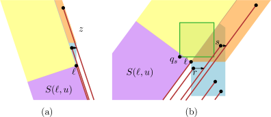
Figure 7: We can find the leaders that can intersect a label from a point in $S(\ell,u)$ by a series of horizontal ray shooting queries.

The only question remaining is how to find the next leader $\gamma_{s}$ given point $r$. To this end we maintain a second data structure. We use a shear transformation such that the leaders are all vertical. We then build a dynamic data structure $\mathcal{D}$ for horizontal ray shooting queries among vertical half-lines. Such a data structure can be build in $O(n\log n)$ time, and allows for $O(\log n)$ updates and queries. See for example[11], although much simpler solutions are possible. We can update $\mathcal{D}$ for the next configuration $\mathcal{C}^{\prime}_{\ell{}E}$ in $O(\log n)$ time, since only a constant number of points change from being labeled internally to labeled externally and vice versa.

Hence, after $O(n\log n)$ time preprocessing, we can compute the “rightmost” point conflicting with each configuration $\mathcal{C}_{\ell{}E}$ in $O(\log n)$ time. The total time required to compute $\Psi^{\prime}(p,\mathcal{C}_{\ell{}E},\mathcal{C}_{uF})$, for all points $p\in S(\ell,u)$, is thus $O(|\mathcal{U}_{\ell{}E}||\mathcal{U}_{uF}|+(n+|\mathcal{U}_{\ell{}E}|+|\mathcal{U}_{uF}|)\log n)$.

After precomputing all values of $f$, the dynamic programming takes $O(n^{3}|\mathcal{U}_{\ell{}E}||\mathcal{U}_{uF}||\mathcal{U}_{pE}||\mathcal{U}_{pF}|)$ time. We thus obtain a total running time of $O(n^{3}\log n+n^{3}|\mathcal{U}_{\ell{}E}||\mathcal{U}_{uF}||\mathcal{U}_{pE}||\mathcal{U}_{pF}|))$. Using that $|\mathcal{U}_{\ell{}E}|$ and $|\mathcal{U}_{pE}|$ are both at most $O(n^{e^{\prime}(\theta)}+\delta^{e(\theta)})$ (Lemma 10), and that $|\mathcal{U}_{uF}|$ and $|\mathcal{U}_{pF}|$ are at most $O(n^{f^{\prime}(\theta)}+\delta^{f(\theta)})$ (Lemma 11) we can rewrite this to $O(n^{3}(\log n+\iota(n,\delta,\theta)))$, where $\iota(n,\delta,\theta)$ is a term that models how much the subproblems can influence each other. We have

$$\iota(n,\delta,\theta)= n^{2e^{\prime}(\theta)+2f^{\prime}(\theta)} + n^{2e^{\prime}(\theta)+f^{\prime}(\theta)} \delta^{f(\theta)} + n^{e^{\prime}(\theta)+2f^{\prime}(\theta)} \delta^{e(\theta)}$$

$$+ n^{e^{\prime}(\theta)+f^{\prime}(\theta)} \delta^{e(\theta)+f(\theta)} + n^{2e^{\prime}(\theta)} \delta^{2f(\theta)} + n^{2f^{\prime}(\theta)} \delta^{2e(\theta)}$$

$$+ n^{e^{\prime}(\theta)} \delta^{e(\theta)+2f(\theta)} + n^{f^{\prime}(\theta)} \delta^{2e(\theta)+f(\theta)} + \delta^{2e(\theta)+2f(\theta)}.$$

For $\delta=O(n)$, this gives us a worst case running time varying between $O(n^{3}\log n)$ and $O(n^{15})$. We conclude:

Proposition 12.

Given a set $\mathcal{P}$ of $n$ points and an angle $\theta$, we can compute a labeling of $\mathcal{P}$ that maximizes the number of internal labels in $O(n^{3}(\log n+\iota(n,\delta,\theta)))$ time and $O(n^{2}\sqrt{\iota(n,\delta,\theta)})$ space, where $\delta=\min\{n,1/d_{\min}\}$ for the minimum distance $d_{\min}$ in $\mathcal{P}$, and $\iota(n,\delta,\theta)$ models how much subproblems can influence each other.

3.3 An Improved Bound on the Number of Configurations

The analysis above, together with the fact that $e(\theta)$ and $f(\theta)$ are both at most three, gives us a worst case running time of $O(n^{15})$. We now study the situation a bit more carefully, and show that the number of interesting configurations is much smaller. More specifically, that we can replace $e(\theta)$ and $S_{F}(\theta)$ by a quantities $e^{*}(\theta)$ and $f^{*}(\theta)$ that are both at most one. This significantly improves the running time of our algorithm.

We start by observing that for some points $q$ in $E(\ell)$, the subproblem $S(\ell,u)$ does not have a labeling compatible with $q$, irrespective of whether $q$ is labeled internally or externally. Let $Q(\ell)$ denote the set of such points. It follows that we can restrict ourselves to labelings, and thus configurations, that do not contain points from $Q(\ell)$. Let $\mathcal{U}^{*}_{\ell{}E}=\{(\mathcal{I},\mathcal{E})\mid(\mathcal{I},\mathcal{E})\in\mathcal{U}_{\ell{}E}\land\mathcal{I}\subseteq Y(\ell)\}$ denote this subset of configurations, where $Y(\ell)=E(\ell)\setminus Q(\ell)$.

Lemma 13.

For every configuration $(\mathcal{I},\mathcal{E})\in\mathcal{U}^{*}_{\ell{}E}$, the set $\mathcal{I}$ has size at most two.

Proof.

By Corollary 7 there are at most $e(\theta)$ points in $E(\ell)$ that can be labeled internally simultaneously. Hence $|\mathcal{I}|\leq e(\ell)$. For $\theta\in[0,3\pi/2]\cup[7\pi/8,2\pi]$ we have $e(\theta)\leq 2$, and thus the lemma follows immediately. For $\theta\in(7\pi/8,2\pi)$ we have $e(\theta)\leq 3$. We prove this remaining case by contradiction.

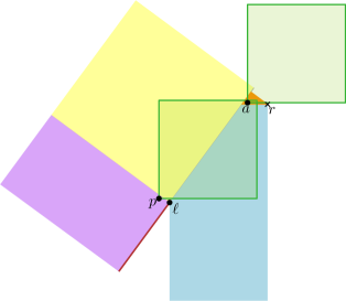
Figure 8: $S(\ell,u)$ is incompatible with any point $a\in\tilde{B_{\ell}}\cap\tilde{L_{r}}\cap T_{r}$ (the orange region).

Assume that $\theta\in(7\pi/8,2\pi)$, and that $\mathcal{I}=\{a,b,c\}$. Since the region $E(\ell)$ has size $1\times 3$, it follows that one of these points, say point $a$, lies in the triangular region $\tilde{B_{\ell}}\cap\tilde{L_{r}}\cap T_{r}$, with $r=(\ell_{x}+1,\ell_{y}+1)$. See Fig. 8. Let $p$ be a point in $S(\ell,u)$ whose label intersects $\lambda_{a}$. Using that $\theta\in(7\pi/8,2\pi)$ it follows that $p$ is to the bottom-left of $a$. Since the labels are to the top-right of a point, we then obtain that $a\in\lambda_{p}$. Therefore, the leader $\gamma_{a}$ also intersects $\lambda_{p}$. So, both the label and the leader of $a$ interfere with $S(\ell,u)$, and thus $a\not\in X(\ell)$ and thus also not in $\mathcal{I}\subseteq X(\ell)$. Contradiction. ∎

Lemma 14.

Let $p$ be a point in $S(\ell,u)$, and let $(\mathcal{I},\mathcal{E})\in\mathcal{U}^{*}_{\ell{}E}$. The label of $p$ intersects at most one label $\lambda_{q}$ of a point $q\in\mathcal{I}$.

Proof.

When $|\mathcal{I}|\leq 1$, the lemma is trivially true. By Lemma 13, we otherwise have $|\mathcal{I}|\leq 2$ and $\theta\in(0,\pi/4)\cup(3\pi/2,2\pi)$. Let $\mathcal{I}=\{a,b\}$. For the case $\theta\in(0,\pi/4)$, assume w.l.o.g. that $b$ is the leftmost point. Since $a$ and $b$ are both in $\mathcal{I}$, their labels are disjoint, and thus we have $b_{x}+1<a_{x}$ (See Fig. 9(a)). Furthermore, we have $p_{y}\geq\ell_{y}\geq b_{y}$. Since $\lambda_{p}$ intersects $\lambda_{b}$, but $p\not\in\lambda_{b}$ this means $p_{x}<b_{x}$. Since $\lambda_{p}$ has width one, it thus cannot intersect $\lambda_{a}$.

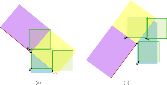
Figure 9: Point $p\in S(\ell,u)$ can intersect only one label of a point in $E(\ell)$.

For the case $\theta\in(3\pi/2,2\pi)$ we use a similar argument. Assume w.l.o.g. that $a$ is the topmost point, and thus $a_{y}>b_{y}+1$. See Fig. 9(b). Since $p\in S(\ell,u)$, $\lambda_{p}$ intersects $\lambda_{a}$, and $a\not\in\lambda_{p}$ we have that $p$ is to the top-left of $a$. And thus, $p_{y}>a_{y}>b_{y}+1$. The label of $b$ has height at most one, and thus cannot intersect $\lambda_{p}$. ∎

Lemma 15.

Let $\mathcal{C}=(\{a,b\},\mathcal{E})\in\mathcal{U}^{*}_{\ell{}E}$, where $a$ is to the right of $b$ if $\theta\in(0,\pi/4)$, and to the top of $b$ if $\theta\in(3\pi/4,2\pi)$. Point $b$ uniquely determines $a$.

Proof.

We prove this by contradiction. Assume that there is another configuration $\mathcal{C}^{\prime}=(\{a^{\prime},b\},\mathcal{E}^{\prime})\in\mathcal{U}^{*}_{\ell{}E}$, such that $a^{\prime}\in Y(\ell)$ is to the right of $b$ in case $\theta\in(0,\pi/4)$, or above $b$ in case $\theta\in(3\pi/4,2\pi)$.

The points $a$ and $b$ can influence the labeling of $S(\ell,u)$. Hence, their labels intersect with labels of points in $S(\ell,u)$. By Lemma 14 $\lambda_{a}$ and $\lambda_{b}$ cannot both intersect the same label of a point in $S(\ell,u)$. So, let $p$ be the point whose label intersects $\lambda_{a}$, and let $q$ be the point whose label intersects $\lambda_{b}$. See Fig. 10.

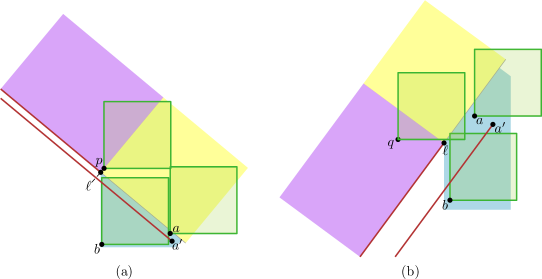
Figure 10: The points $a,a^{\prime}$, and $b$ in $E(\ell)$ and the label(s) in $S(\ell,u)$ they intersect. (Fig (a) is not on scale.)

We start with the case $\theta\in(0,\pi/4)$. Point $a$ is to the right of $b$, and $\lambda_{a}$ and $\lambda_{b}$ are disjoint. Hence, $a_{x}>b_{x}+1$. Since $\lambda_{p}$ intersects $\lambda_{a}$, and $p\not\in\lambda_{b}$, it follows that $p$ lies above $\lambda_{p}$. Hence $p_{y}>b_{y}+1$. Again using that $\lambda_{p}$ intersects $\lambda_{a}$, it then also follows that $a_{y}>b_{y}$. Using the same argument we get $a^{\prime}_{y}>b_{y}$. Now in the configuration $\mathcal{C}$, point $a^{\prime}$ is labeled externally. However, this means its leader intersects $\lambda_{b}$. Hence, $\mathcal{C}\not\in\mathcal{U}^{*}_{\ell{}E}$. Contradiction.

For the case $\theta\in(3\pi/2,2\pi)$ we have that $b_{y}+1<a_{y}$. As in the proof of Lemma 13 we have that $a_{y}<\ell_{y}+1$, and hence $b_{y}<\ell_{y}$. Using that $\lambda_{q}$ does not intersect $\gamma_{\ell}$, we have $q_{y}>\ell_{y}$. Since $q\not\in\lambda_{b}$ it follows that $q_{x}<b_{x}$. In configuration $\mathcal{C}^{\prime}$, $\lambda_{a^{\prime}}$ and $\lambda_{b}$ are also pairwise disjoint. It then follows that $a^{\prime}$ is to the top-right of $b$. In the configuration $\mathcal{C}=(\{a,b\},\mathcal{E})$, point $a^{\prime}$ is labeled externally. However, this means its leader intersects $\lambda_{b}$. Hence, $\mathcal{C}\not\in\mathcal{U}^{*}_{\ell{}E}$. Contradiction. ∎

Corollary 16.

The number of configurations in $\mathcal{U}^{*}_{\ell{}E}$ is at most $O(n^{e^{\prime}(\theta)}+\delta^{e^{*}(\theta)})$, where $e^{*}(\theta)=\min\{1,e(\theta)\}$.

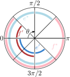
Figure 11: A depiction of the upper bounds on $e^{*},e^{\prime},s^{*}F,$ and $f^{\prime}$ as a function of $\theta$.

We can again use a symmetric argument for the number of configurations in $\tilde{T_{u}}$. Figure 11 gives a graphical summary of these results. We now redefine $\iota(n,\delta,\theta)$ as

$$\iota(n,\delta,\theta)= n^{2e^{\prime}(\theta)+2f^{\prime}(\theta)} + n^{2e^{\prime}(\theta)+f^{\prime}(\theta)} \delta^{f^{*}(\theta)} + n^{e^{\prime}(\theta)+2f^{\prime}(\theta)} \delta^{e^{*}(\theta)}$$

$$+ n^{e^{\prime}(\theta)+f^{\prime}(\theta)} \delta^{e^{*}(\theta)+f^{*}(\theta)} + n^{2e^{\prime}(\theta)} \delta^{2f^{*}(\theta)} + n^{2f^{\prime}(\theta)} \delta^{2e^{*}(\theta)}$$

$$+ n^{e^{\prime}(\theta)} \delta^{e^{*}(\theta)+2f^{*}(\theta)} + n^{f^{\prime}(\theta)} \delta^{2e^{*}(\theta)+f^{*}(\theta)} + \delta^{2e^{*}(\theta)+2f^{*}(\theta)}.$$

and obtain the following result, which is at most $O(n^{7})$ for $\delta=O(n)$:

Theorem 17.

Given a set $\mathcal{P}$ of $n$ points and an angle $\theta$, we can compute a labeling of $\mathcal{P}$ that maximizes the number of internal labels in $O(n^{3}(\log n+\iota(n,\delta,\theta)))$ time and $O(n^{2}\sqrt{\iota(n,\delta,\theta)})$ space, where $\delta=\min\{n,1/d_{\min}\}$ for the minimum distance $d_{\min}$ in $\mathcal{P}$, and $\iota(n,\delta,\theta)$ models how much subproblems can influence each other. More formally,

$$\iota(n,\delta,\theta)= n^{2e^{\prime}(\theta)+2f^{\prime}(\theta)} + n^{2e^{\prime}(\theta)+f^{\prime}(\theta)}\delta^{f^{*}(\theta)} + n^{e^{\prime}(\theta)+2f^{\prime}(\theta)}\delta^{e^{*}(\theta)}$$

$$+ n^{e^{\prime}(\theta)+f^{\prime}(\theta)}\delta^{e^{*}(\theta)+f^{*}(\theta)} + n^{2e^{\prime}(\theta)}\delta^{2f^{*}(\theta)} + n^{2f^{\prime}(\theta)}\delta^{2e^{*}(\theta)}$$

$$+ n^{e^{\prime}(\theta)}\delta^{e^{*}(\theta)+2f^{*}(\theta)} + n^{f^{\prime}(\theta)}\delta^{2e^{*}(\theta)+f^{*}(\theta)} + \delta^{2e^{*}(\theta)+2f^{*}(\theta)},$$

where $e^{*}(\theta),f^{*}(\theta),e^{\prime}(\theta)$, and $f^{\prime}(\theta)$ are all at most one.

4 Extensions

So far, we have considered a stylized version of the question we set out to solve. In this section we discuss how our solution may be adapted and extended, depending on the exact requirements of the application.

4.1 Optimizing the direction

Rather than fixing the direction for the leaders in advance, we may be willing to let the algorithm specify the optimal orientation that maximizes the number of points that can be labeled internally. Or, perhaps we wish to compute a chart that plots the maximum number of internally labeled points as a function of the leader orientation $\theta$, leaving the final decision to the judgement of the user.

In both scenarios, we need to efficiently iterate over all possible orientations. We adapt our method straightforwardly. Let $Q$ be the set of all $4n$ corner points of all potential labels. For every pair $p,q\in Q$ consider the slope $\theta_{p,q}$ of the line through $p$ and $q$. All values $\theta_{p,q}$ partition all possible angles into $O(n^{2})$ intervals. For all values $\theta$ in the same interval $J$, any leader $\gamma_{p}$ intersects the same set of potential labels, so the optimal set of internal labels is constant throughout $J$. We compute it separately for each interval.

By applying Theorem 17, we achieve a total of $O(n^{2}\cdot n^{3}(\log n+\iota(n,\delta,\theta)))=O(n^{5}(\log n+\iota(n,\delta,\theta)))$ time to compute the optimal labelings for all orientations, or to optimize the orientation by performing a simple linear scan.

4.2 Routing the outer leaders

Once the core combinatorial problem of deciding which points have to be labeled internally is solved, it remains to route the outer leaders and place the external labels. Since our goal in this paper is to maximize the number of internally labeled points, we are only interested in finding a valid labeling, in which neither labels nor leaders intersect each other. Let us assume that $\theta\in[0,\pi/2]\cup[3\pi/2,2\pi]$, i.e., all external labels are oriented to the left. The case of labels oriented to the right is symmetric. We consider the leaders in counterclockwise order around the boundary of $\mathcal{M}$ and place them one by one starting with the topmost leader. The first label is placed with its lower right corner anchored at the endpoint of its inner leader. For all subsequent labels we test if the label anchored at the endpoint of the inner leader intersects the previously placed label. If there is no intersection, we use that label position. Otherwise, we draw an outer leader extending horizontally to the left starting from the endpoint of the inner leader until the label can be placed without overlap. Obviously this algorithm takes only linear time. Figure 12 shows the resulting labelings for four different slopes. We note that depending on the slope $\theta$ of the inner leaders other methods for routing the outer leaders might yield more pleasing external labelings. This is, however, beyond the scope of this paper.

(a) $\theta=0$

(b) $\theta=\pi/3$

(c) $\theta=7\pi/4$

(d) $\theta=11\pi/6$

Figure 12: Examples for routing the outer leaders and placing the external labels for different slopes.

4.3 Non-square labels

Square labels are not very realistic in most map-labeling applications. Their use is justified by the observation that if all labels are homothetic rectangles, we can scale the plane in one dimension to obtain square labels without otherwise changing the problem. Nonetheless, reality is not quite that simple, for two reasons: firstly, the scaling does alter inter-point distances, so if we wish to parametrize our solution by $d_{\min}$ we need to take this into account. Secondly, in real-world applications, labels may arguably have the same height, but not usually the same width.

If all labels are homothetic rectangles with a height of $1$ and a width of $w$, scaling the plane by a factor $1/w$ in the horizontal direction potentially decreases the closest interpoint distance by the same factor. Now, the number of points in a unit-area region that do not contain each other’s potential labels is bounded by $\delta w$, immediately yielding a result of $O(n^{3}(\log n+\iota(n,\delta w,\theta)))$ using exactly the same approach.

When all labels have equal heights but may have arbitrary widths, we conjecture that a variation of our approach will still work, but a careful analysis of the intricacies involved is required. If the labels may also have arbitrary heights the problem is open. It is unclear if there is a polynomial time solution in this case.

4.4 Obstacles

In this paper, we have considered only abstract point sets to be labeled, using leaders that are allowed to go anywhere, as long as they do not intersect any internal labels. While this is justified in some applications (e.g., in anatomical drawings, it is common practice to ignore the drawing when placing the leaders, as they are very thin and do not occlude any part of the drawing), in others this may be undesirable (in certain map styles, leaders may be confused for region boundaries or linear features). As a solution, we may identify a set of polygonal obstacles in the map, that cannot be intersected by leaders or internal labels.

In this setting, obviously not every input has a valid labeling: a point that lies inside an obstacle can never be labeled, or obstacles may surround points or force points into impossible configurations in more complex ways. Nonetheless, we can test whether an input has a valid labeling and if so, compute the labeling that maximizes the number of internal labels in polynomial time with our approach.

The main idea is to preprocess the input points in a similar way as in the beginning of Section 3. Whenever a point has a potential leader that intersects an obstacle, it must be labeled internally; similarly, whenever a point has a potential internal label that intersects an obstacle, it must be labeled externally. If we include such “forced” leaders or labels into our set of obstacles and apply this approach recursively, we will either find a contradiction or be left with a set of points whose potential leaders and potential internal labels do not intersect any obstacle, and we can apply our existing algorithm on this point set.

The same approach may be used for point sets that are not in general position: if we disallow leaders that pass through other points, they are forced to be labeled internally. Note that this again may result in situations where no valid labeling exists.

Acknowledgments

M.L. and F.S. are supported by the Netherlands Organisation for Scientific Research (NWO) under grant 639.021.123 and 612.001.022, respectively.

References

- [1] P. K. Agarwal, M. van Kreveld, and S. Suri. Label placement by maximum independent set in rectangles. Comput. Geom. Theory Appl., 11(3-4):209–218, 1998.
- [2] M. Bekos, M. Kaufmann, M. Nöllenburg, and A. Symvonis. Boundary labeling with octilinear leaders. Algorithmica, 57:436–461, 2010.
- [3] M. Bekos, M. Kaufmann, D. Papadopoulos, and A. Symvonis. Combining traditional map labeling with boundary labeling. In Proc. 37th Int. Conf. on Current Trends in Theory and Practice of Computer Science (SOFSEM’11), volume 6543 of LNCS, pages 111–122, 2011.
- [4] M. A. Bekos, M. Kaufmann, and A. Symvonis. Efficient labeling of collinear sites. J. Graph Algorithms Appl., 12(3):357–380, 2008.
- [5] M. A. Bekos, M. Kaufmann, A. Symvonis, and A. Wolff. Boundary labeling: Models and efficient algorithms for rectangular maps. Comput. Geom. Theory Appl., 36(3):215–236, 2007.
- [6] M. Benkert, H. Haverkort, M. Kroll, and M. Nöllenburg. Algorithms for multi-criteria boundary labeling. J. Graph Algorithms and Appl., 13(3):289–317, 2009.
- [7] P. Chalermsook and J. Chuzhoy. Maximum independent set of rectangles. In Discrete Algorithms (SODA’09), pages 892–901, 2009.
- [8] M. de Berg, M. van Kreveld, M. Overmars, and O. Schwarzkopf. Computational Geometry: Algorithms and Applications. Springer-Verlag, Berlin, Germany, 2nd edition, 2000.
- [9] M. Formann and F. Wagner. A packing problem with applications to lettering of maps. In Computational Geometry (SoCG’91), pages 281–288. ACM, 1991.
- [10] A. Gemsa, J.-H. Haunert, and M. Nöllenburg. Boundary-labeling algorithms for panorama images. In Advances in Geographic Information Systems (SIGSPATIAL GIS’11), pages 289–298. ACM, 2011.
- [11] Y. Giora and H. Kaplan. Optimal dynamic vertical ray shooting in rectilinear planar subdivisions. ACM Trans. Algorithms, 5(3):28:1–28:51, July 2009.
- [12] Z.-D. Huang, S.-H. Poon, and C.-C. Lin. Boundary labeling with flexible label positions. In Algorithms and Computation (WALCOM’14), volume 8344 of LNCS, pages 44–55. Springer, 2014.
- [13] E. Imhof. Positioning names on maps. The American Cartographer, 2(2):128–144, 1975.
- [14] M. Kaufmann. On map labeling with leaders. In S. Albers, H. Alt, and S. Näher, editors, Festschrift Mehlhorn, volume 5760 of LNCS, pages 290–304. Springer-Verlag, 2009.
- [15] P. Kindermann, B. Niedermann, I. Rutter, M. Schaefer, A. Schulz, and A. Wolff. Two-sided boundary labeling with adjacent sides. In Algorithms and Data Structures (WADS’13), volume 8037 of LNCS, pages 463–474, 2013.
- [16] G. W. Klau and P. Mutzel. Optimal labeling of point features in rectangular labeling models. Mathematical Programming, 94(2):435–458, 2003.
- [17] M. Löffler and M. Nöllenburg. Shooting bricks with orthogonal laser beams: A first step towards internal/external map labeling. In Canadian Conf. Computational Geometry (CCCG ’10), pages 203–206. University of Manitoba, 2010.
- [18] J. Marks and S. Shieber. The computational complexity of cartographic label placement. Technical report, Harvard University, 1991.
- [19] K. Mehlhorn and S. Näher. Dynamic fractional cascading. Algorithmica, 5(1–4):215–241, 1990.
- [20] M. Nöllenburg, V. Polishchuk, and M. Sysikaski. Dynamic one-sided boundary labeling. In Advances in Geographic Information Systems (SIGSPATIAL GIS’10), pages 310–319, November 2010.
- [21] A. Reimer and M. Rylov. Point-feature lettering of high cartographic quality: A multi-criteria model with practical implementation. In EuroCG’14, Ein-Gedi, Israel, 2014.
- [22] M. van Kreveld, T. Strijk, and A. Wolff. Point labeling with sliding labels. Comput. Geom. Theory Appl., 13(1):21–47, 1999.
- [23] A. Wolff and T. Strijk. The map labeling bibliography.