Localization Analysis of an Energy-Based Fourth-Order Gradient Plasticity Model

Abstract

The purpose of this paper is to provide analytical and numerical solutions of the formation and evolution of the localized plastic zone in a uniaxially loaded bar with variable cross-sectional area. An energy-based variational approach is employed and the governing equations with appropriate physical boundary conditions, jump conditions, and regularity conditions at evolving elasto-plastic interface are derived for a fourth-order explicit gradient plasticity model with linear isotropic softening. Four examples that differ by regularity of the yield stress and stress distributions are presented. Results for the load level, size of the plastic zone, distribution of plastic strain and its spatial derivatives, plastic elongation, and energy balance are constructed and compared to another, previously discussed non-variational gradient formulation.

1 Introduction

The presence of a softening branch of the stress-strain curve, usually caused by initiation, propagation and coalescence of defects such as micro-cracks or micro-voids, is a phenomenon typical of quasi-brittle materials. Softening often leads to localization of strain into narrow bands whose width is related to an intrinsic length dictated by the heterogeneities of the material microstructure. Softening can be conveniently incorporated into damage models, but can also be described by plasticity with a negative hardening modulus. However, constitutive models within the classical continuum framework of simple materials do not contain any length scale reflecting the typical size of microstructural features. Therefore, the localization processes due to softening are not described properly and mathematical models lead to ill-posed problems accompanied by localization of strain into subdomains of zero volume and consequently to vanishing dissipation. Various enrichments incorporating some information about the material heterogeneity have been developed. They utilize, for example, additional kinematic variables, weighted spatial averages, higher-order gradients, or rate-dependent terms; see e.g. the comparative studies and review papers by de Vree et al. (1995), Jirásek (1998), Peerlings et al. (2001), Jirásek and Rolshoven (2003), Bažant and Jirásek (2002), Jirásek and Rolshoven (2009a) and Jirásek and Rolshoven (2009b). These techniques on the one hand preclude localization and loss of ellipticity of the governing equations, but on the other hand significantly complicate the overall analysis. For instance, in the case of higher-order gradient models, the regularity conditions of internal variables at the evolving elasto-plastic interface are not easy to characterize.

The present paper is devoted to the investigation of the Aifantis explicit fourth-order gradient plasticity model, cf. e.g. Zbib and Aifantis (1988) or Mühlhaus and Aifantis (1991), under conditions leading to non-uniform stress fields. To keep the analysis transparent, we confine ourselves to one-dimensional tension tests and perform our analysis in the framework of the so-called energetic solutions introduced in an abstract setting in Mielke and Theil (2004) and in the context of finite-strain plasticity in Mielke (2003), generalizing earlier variational formulations of damage (Francfort and Marigo, 1993) and fracture (Francfort and Marigo, 1998). Building on this basis, we will derive the governing equations and appropriate boundary and jump conditions. In particular, the often questioned regularity conditions for internal variables at the elasto-plastic interface will emerge naturally in a consistent and unified way. Detailed solutions for four different test problems with various regularity of the yield stress and stress distributions will be presented and compared to results obtained from the standard non-variational gradient formulation available in Jirásek et al. (2010). The present work can also be viewed as a continuation and extension of results provided in our previous paper (Jirásek et al., 2013), where the second-order gradient plasticity model was investigated. The main difference from our previous work is that now we treat a more complicated model with higher-order regularity requirements on internal variables and more intricate conditions at the elasto-plastic interface. In addition, we approach the problem utilizing the nowadays standard variational framework for rate-independent evolution.

This study is also closely related to several one-dimensional studies into energy-based second-order gradient models of strain-softening damage and plasticity. In particular, Pham et al. (2011) performed a detailed analysis of stability and bifurcation of localized and homogenous states, obtained in the closed form, for a parameterized family of gradient damage models. These results were later refined by Pham and Marigo (2013), who studied size effects and snap-back behaviour at the structural scale predicted by the same group of damage models. The combination of damage and plasticity has been the subject of recent contributions by Del Piero et al. (2013) and Alessi et al. (2014), with the emphasis on the competition between brittle and ductile failure; the former work, as well as Milašinović (2004), also contain a validation against experimental data. Theoretical results of fracture and plasticity as $\Gamma$-limits of damage models within one-dimensional setting are described in Iurlano (2013), and non-local damage or fracture analyses in bars under tension are discussed in Jirásek and Zeman (2015) and Lellis and Royer-Carfagni (2001); all these works also employ a variational formulation. Our analysis extends these contributions by treating a model regularized by the fourth derivative of internal variables and by deriving the regularity of internal variables directly from energy-minimization arguments, rather than enforcing them through additional boundary conditions at the moving elastic-inelastic interfaces.

The energetic formulation for rate-independent processes comprises several steps and relies on two principles. In the abstract setting (Mielke, 2006), the state of the system within a fixed time horizon $T$ is described in terms of a ”non-dissipative” field $\boldsymbol{u}(t,\boldsymbol{x})$, $\boldsymbol{u}(t)\in\mathcal{U}$, $\boldsymbol{x}\in\Omega$, where $\Omega$ denotes the spatial domain, and a ”dissipative” field $\boldsymbol{z}(t,\boldsymbol{x})$, $\boldsymbol{z}(t)\in\mathcal{Z}$, which specifies the irreversible processes at time $t\in[0,T]$. The state of the system is fully characterized by the state variables $\boldsymbol{q}(t,\boldsymbol{x})$, $\boldsymbol{q}(t)=(\boldsymbol{u}(t),\boldsymbol{z}(t))\in\mathcal{Q}=\mathcal{U}\times\mathcal{Z}$. Typically, $\boldsymbol{u}$ is the displacement field and $\boldsymbol{z}$ is the field of internal variables related to the inelastic phenomena, such as plastic strain or damage. Further, we consider the total free (Helmholtz) energy of the body $\mathcal{E}:[0,T]\times\mathcal{Q}\rightarrow\mathbb{R}\cup\{+\infty\}$ together with the dissipation distance $\mathcal{D}:\mathcal{Z}\times\mathcal{Z}\rightarrow\mathbb{R}\cup\{+\infty\}$ which specifies the minimum amount of energy spent by the continuous transition from state $\boldsymbol{z}^{(1)}$ to state $\boldsymbol{z}^{(2)}$. For notational convenience, we will sometimes refer to the dissipation distance by $\mathcal{D}(\boldsymbol{q}^{(1)},\boldsymbol{q}^{(2)})$ instead of $\mathcal{D}(\boldsymbol{z}^{(1)},\boldsymbol{z}^{(2)})$. Then, the process $\boldsymbol{q}:[0,T]\rightarrow\mathcal{Q}$ is an energetic solution to the initial-value problem described by $(\mathcal{E},\mathcal{D},\boldsymbol{q}_{0})$ if it satisfies

1. Global stability: for all $t\in[0,T]$ and for all $\widehat{\boldsymbol{q}}\in\mathcal{Q}$

   $$\mathcal{E}(t,\boldsymbol{q}(t))\leq\mathcal{E}(t,\widehat{\boldsymbol{q}})+\mathcal{D}(\boldsymbol{q}(t),\widehat{\boldsymbol{q}})$$ (S)

   which ensures that the solution minimizes the sum $\mathcal{E}+\mathcal{D}$,

2. Energy equality: for all $t\in[0,T]$

   $$\mathcal{E}(t,\boldsymbol{q}(t))+\mathrm{Var}_{\mathcal{D}}(\boldsymbol{q};0,t)=\mathcal{E}(0,\boldsymbol{q}(0))+\int_{0}^{t}\mathcal{P}(s)\,\mbox{d}s$$ (E)

   which expresses energy balance in terms of the internal energy, dissipated energy $\mathrm{Var}_{\mathcal{D}}$, and time-integrated power of external forces $\mathcal{P}$,

3. Initial condition:

   $$\boldsymbol{q}(0)=\boldsymbol{q}_{0}$$ (I)

The dissipation along a process $\boldsymbol{q}$ is expressed as

$$\mathrm{Var}_{\mathcal{D}}(\boldsymbol{q};0,t)=\sup\left\{\sum_{i=1}^{n}\mathcal{D}(\boldsymbol{q}(t_{i-1}),\boldsymbol{q}(t_{i}))\right\}$$ (1)

where the supremum is taken over all $n\in\mathbb{N}$ and all partitions of the time interval $[0,t]$, $0=t_{0}<t_{1}<\dots<t_{n}=t$. Together, the two principles (S) and (E) along with initial condition (I) naturally give rise to an
Incremental problem: for $k=1,\ldots,N$

$$\boldsymbol{q}(t_{k})\in\underset{\widehat{\boldsymbol{q}}\in\mathcal{Q}}{\mbox{Arg min}}\left[\mathcal{E}(t_{k},\widehat{\boldsymbol{q}})+\mathcal{D}(\boldsymbol{q}(t_{k-1}),\widehat{\boldsymbol{q}})\right]$$ (IP)

amenable to a numerical solution, in which each step is realized as a minimization problem, e.g. Ortiz and Stainier (1999); Carstensen et al. (2002); Petryk (2003). The main conceptual difficulty with this incremental problem is that it represents a global minimization, which is computationally cumbersome and physically difficult to justify for non-convex energies. It is reasonable, however, to assume that stable solutions to (IP) are associated with local minima; for comparative studies into evolution driven by local and global energy minimization see e.g. Mielke (2011); Braides (2014); Roubíček (2015). On the other hand, the variational approach offers many advantages, among which we highlight that it provides a unified setting for the analysis, allows for discontinuities in space, incorporates the governing laws with boundary conditions and provides regularity conditions at the elasto-plastic interface.

For the uniaxial displacement-controlled tension test, we can further specify all the quantities introduced above in more detail. Displacement $u(t,x)$, where we have used the light face letter since $u$ is now a scalar field, as a function of the spatial coordinate $x\in\Omega\subset\mathbb{R}$, represents the ”non-dissipative” component; the total linearized strain is simply the spatial derivative $u^{\prime}(t,x)=\partial u(t,x)/\partial x$. The ”dissipative” variables, describing the irreversible processes, are plastic strain $\varepsilon_{p}(t,x)$ and cumulative plastic strain $\kappa(t,x)$, i.e. $\boldsymbol{z}(t,x)=(\varepsilon_{p}(t,x),\kappa(t,x))$. The corresponding function spaces are as follows:

$$u\in V_{u}(t) =\left\{\widehat{u}\in W^{1,2}(\Omega)\,|\,\widehat{u}=u_{D}(t)\mbox{ on }\partial\Omega\mbox{ in the sense of traces}\right\}$$ (2a)

$$\varepsilon_{p}\in V_{\varepsilon_{p}} =W^{2,2}(\Omega)$$ (2b)

$$\kappa\in V_{\kappa} =\left\{\widehat{\kappa}\in W^{2,2}(\Omega)\,|\,\widehat{\kappa}\geq 0\right\}$$ (2c)

where $u_{D}(t)$ denotes prescribed displacements on the boundary (specifying the Dirichlet boundary condition) and $W^{k,2}$ stands for the space of all Lebesgue square-integrable functions with square-integrable generalized derivatives up to order $k$; later on, we will employ a subset $W^{k,2}_{0}$ consisting of functions vanishing at the boundary, for details we refer to e.g. Evans (2010). Consequently, we identify $\mathcal{U}=V_{u}(t)$, which now depends on time (due to the time-dependent values presented on the boundary), $\mathcal{Z}=V_{\varepsilon_{p}}\times V_{\kappa}$, $\mathcal{Q}=\mathcal{U}\times\mathcal{Z}=V_{u}(t)\times V_{\varepsilon_{p}}\times V_{\kappa}$, and define the total free energy of the body

$$\mathcal{E}(t,u,\varepsilon_{p},\kappa)=\int_{\Omega}\frac{1}{2}EA(u^{\prime}-\varepsilon_{p})^{2}\,\mbox{d}x+\int_{\Omega}\frac{1}{2}HA(\kappa^{2}-l^{4}\kappa^{\prime\prime 2})\,\mbox{d}x-\int_{\Omega}Abu\,\mbox{d}x$$ (3)

and the dissipation distance

$$\mathcal{D}(\boldsymbol{z}^{(1)},\boldsymbol{z}^{(2)})=\left\{\begin{aligned} &\int_{\Omega}A\sigma_{0}|\varepsilon_{p}^{(2)}-\varepsilon_{p}^{(1)}|\,\mbox{d}x&&\mbox{ if }\kappa^{(2)}=\kappa^{(1)}+|\varepsilon_{p}^{(2)}-\varepsilon_{p}^{(1)}|\mbox{ in }\Omega\\ &+\infty&&\mbox{ otherwise}\end{aligned}\right.$$ (4)

Quantities appearing in the definitions of energies represent the Young modulus $E$ [Pa], softening modulus $H<0$ [Pa], characteristic length of the material $l$ [m], initial yield stress $\sigma_{0}$ [Pa], a function describing the distribution of the cross-sectional area along the bar $A(x)$ [m²], and prescribed body force density $b(x)$ [N/m³]. For completeness, let us note that the power of external forces in (E) has the form $\displaystyle{\mathcal{P}(s)=F(s)\dot{u}_{D}(s)}$, where $F(s)$ denotes the reaction force as a function of time and the dot stands for the time derivative.

The paper is organized as follows. In Section 2, we will revisit the energetic formulation for the case of monotone loading, i.e. $\dot{u}_{D}(t)\geq 0$, which greatly simplifies the specific form of (S), (E), (I), and (IP) accompanied by (2)–(4). Further, the governing equations with boundary conditions, jump conditions, and regularity conditions at the elasto-plastic interface will be derived for the resulting one-dimensional fourth-order gradient-enriched plasticity model. Sections 3 and 4 are concerned with piecewise constant yield stress and stress distributions, which also represent the only cases amenable to analytical solutions. There, it will be shown that the structural response may, in a certain range, exhibit hardening due to the gradient enrichment despite the softening character of the material model. In Sections 5 and 6, the results for piecewise linear and quadratic stress field distributions will be compared to standard non-variational solutions available in Jirásek et al. (2010). In spite of all the simplifications we will be forced to use numerical solutions. The influence of data variation to the evolution of the plastic zone, its profile and load-displacement diagrams will also be investigated. Finally, in A, the stability conditions for the case of a uniform bar are discussed, and in B, we verify optimality of the obtained regularity conditions at the elasto-plastic interface by an independent argument.

2 Energy-Based Formulation

2.1 General Considerations

For $\mathcal{E}$ and $\mathcal{D}$ given by (3) and (4), minimization in (IP) with respect to $\widehat{\kappa}$ gives $\kappa(t_{k})=\kappa(t_{k-1})+|\widehat{\varepsilon}_{p}-\varepsilon_{p}(t_{k-1})|$. Consequently, (IP) reduces to

$$(u(t_{k}),\varepsilon_{p}(t_{k}))\in\underset{(\widehat{u},\widehat{\varepsilon}_{p})\in V_{u}(t_{k})\times V_{\varepsilon_{p}}}{\mbox{Arg min}} \int_{\Omega}\frac{1}{2}EA(\widehat{u}^{\prime}-\widehat{\varepsilon}_{p})^{2}\,\mbox{d}x$$ (5)

$$+\int_{\Omega}\frac{1}{2}HA[\kappa(t_{k-1})+|\widehat{\varepsilon}_{p}-\varepsilon_{p}(t_{k-1})|]^{2}\,\mbox{d}x$$

$$-\int_{\Omega}\frac{1}{2}HAl^{4}[\kappa^{\prime\prime}(t_{k-1})+|\widehat{\varepsilon}_{p}-\varepsilon_{p}(t_{k-1})|^{\prime\prime}]^{2}\,\mbox{d}x$$

$$+\int_{\Omega}A\sigma_{0}|\widehat{\varepsilon}_{p}-\varepsilon_{p}(t_{k-1})|\,\mbox{d}x-\int_{\Omega}Ab\widehat{u}\,\mbox{d}x$$

cf. also Section 4.3 in Mielke (2003), where the local plasticity model with hardening is discussed. In Eq. (5), spatial derivatives are understood in the sense of distributions. For further considerations, we will restrict ourselves to tensile loading with possible elastic unloading, but never with a reversal of the plastic flow. Then, the plastic strain $\varepsilon_{p}$ and the cumulative plastic strain $\kappa$ are equal, and we can use $\kappa$ as the only internal variable. As a result, instead of the incremental approach given in Eqs. (IP) and (5), it is fully sufficient to consider a total formulation providing a parameterized solution $(u(t),\kappa(t))$ which does not violate the irreversibility constraints. Note that such a parametrization is mathematically justified only when the elastic energy $\mathcal{E}$ is strictly convex in $\boldsymbol{q}$, which implies that the solution is time-continuous for sufficiently regular loading, cf. Mielke and Theil (2004). Later on, instead of imposing the Dirichlet boundary conditions, we prescribe directly the size of the plastic zone as a function of time in order to control the system evolution. This approach automatically entails time-continuity of $\boldsymbol{q}(t)$, which implies satisfaction of the energy balance (Pham et al., 2011; Pham and Marigo, 2013), and also justifies the total formulation.

Taking into account all the above simplifications, the minimization problem in Eq. (5) reduces to

$$(u(t),\kappa(t))\in\underset{(\widehat{u},\widehat{\kappa})\in V_{u}(t)\times V_{\kappa}}{\mbox{Arg min}}\Pi(\widehat{u},\widehat{\kappa})$$ (6)

where

$$\Pi(\widehat{u},\widehat{\kappa})= \int_{\Omega}\frac{1}{2}EA(\widehat{u}^{\prime}-\widehat{\kappa})^{2}\,\mbox{d}x+\int_{\Omega}\frac{1}{2}HA(\widehat{\kappa}^{2}-l^{4}\widehat{\kappa}^{\prime\prime 2})\,\mbox{d}x$$ (7)

$$+\int_{\Omega}A\sigma_{0}\widehat{\kappa}\,\mbox{d}x-\int_{\Omega}Ab\widehat{u}\,\mbox{d}x$$

which resembles a variational inequality of the first kind, due to the requirement $\kappa\geq 0$ in Eq. (2c).

The first variation (Gâteaux derivative) of $\Pi$ furnishes us with the optimality condition

$$\delta\Pi(u,\kappa;\delta u,\delta\kappa)= \int_{\Omega}EA(u^{\prime}-\kappa)(\delta u^{\prime}-\delta\kappa)\,\mbox{d}x+\int_{\Omega}HA(\kappa\delta\kappa-l^{4}\kappa^{\prime\prime}\delta\kappa^{\prime\prime})\,\mbox{d}x$$ (8)

$$+\int_{\Omega}A\sigma_{0}\delta\kappa\,\mbox{d}x-\int_{\Omega}Ab\delta u\,\mbox{d}x\geq 0$$

where $\delta u$ and $\delta\kappa$ are admissible variations satisfying $(u+\delta u,\kappa+\delta\kappa)\in V_{u}(t)\times V_{\kappa}$ (for simplicity, explicit dependence on time $t$ has been dropped). Employing the integration by parts we arrive at

$$\delta\Pi(u,\kappa;\delta u,\delta\kappa)= -\int_{\Omega}[(EA(u^{\prime}-\kappa))^{\prime}+Ab]\delta u\,\mbox{d}x$$ (9)

$$+\int_{\Omega}[HA\kappa-(HAl^{4}\kappa^{\prime\prime})^{\prime\prime}+A\sigma_{0}-EA(u^{\prime}-\kappa)]\delta\kappa\,\mbox{d}x$$

$$+\sum\limits_{\partial\Omega}EA(u^{\prime}-\kappa)n\delta u-\sum\limits_{i}\llbracket EA(u^{\prime}-\kappa)\delta u\rrbracket_{x_{i}}$$

$$-\sum\limits_{\partial\Omega}HAl^{4}\kappa^{\prime\prime}n\delta\kappa^{\prime}+\sum\limits_{i}\llbracket HAl^{4}\kappa^{\prime\prime}\delta\kappa^{\prime}\rrbracket_{x_{i}}$$

$$+\sum\limits_{\partial\Omega}(HAl^{4}\kappa^{\prime\prime})^{\prime}n\delta\kappa-\sum\limits_{i}\llbracket(HAl^{4}\kappa^{\prime\prime})^{\prime}\delta\kappa\rrbracket_{x_{i}}$$

where $\sum_{\partial\Omega}$ denotes the boundary integral, in our one-dimensional setting reduced to the sum over two end points of the interval $\Omega$, and $n$ is the unit outer normal, which equals $-1$ at the left $\partial\Omega_{L}$ and $1$ at the right $\partial\Omega_{R}$ part of the boundary $\partial\Omega=\partial\Omega_{L}\cup\partial\Omega_{R}$. The sums $\sum_{i}$ are taken over all points of possible discontinuity $x_{i}$ and

$$\llbracket f\rrbracket_{x_{i}}=f(x_{i}^{+})-f(x_{i}^{-})=\lim_{x\downarrow x_{i}}f(x)-\lim_{x\uparrow x_{i}}f(x)$$ (10)

represents the jump of function $f(x)$ at $x_{i}$. The necessary condition for a local minimum is non-negativity of the first variation of the functional $\Pi$ for all admissible variations $\delta u$ and $\delta\kappa$, cf. Section 8.4.2 in Evans (2010), or Chapter 5 in Roubíček (2010). Below we show that such an approach leads to a consistent set of governing equations, namely the equilibrium equations, complementarity conditions of the plastic flow, boundary conditions, and regularity conditions at the elasto-plastic interfaces. Analysis of the second variation (second-order Gâteaux derivative), which is related to stability of the solution (S), is postponed to A.

2.2 Governing Equations

Since $u+\delta u\in V_{u}$, we have $\delta u\in W^{1,2}_{0}(\Omega)$, meaning that $\delta u$ is arbitrary inside $\Omega$ with zero trace on the physical boundary $\partial\Omega$. Thus the expression multiplying $\delta u$ in the first line of (9) must vanish, providing us with the static equilibrium condition

$$(EA(u^{\prime}-\kappa))^{\prime}+Ab=0\mbox{ in }\Omega$$ (11)

Here, $u^{\prime}$ corresponds to the total strain, $u^{\prime}-\kappa$ is the elastic strain, and $EA(u^{\prime}-\kappa)$ is the axial force, which is required to be continuous according to the third line of (9), because $\delta u$ is arbitrary inside $\Omega$. Due to the zero trace of $\delta u$, the sum over boundary points in the third line of (9) vanishes.

Since $\kappa+\delta\kappa\in V_{\kappa}$, variations $\delta\kappa$ cannot be completely arbitrary. Let us define the plastic zone as the open set $\mathcal{I}_{p}=\{x\in\Omega\,|\,\kappa(x)>0\}$, i.e., as the support of $\kappa$, and the elastic zone as the open set $\mathcal{I}_{e}=\{x\in\Omega\,|\,\kappa(x)=0\}$. In $\mathcal{I}_{p}$, the variation $\delta\kappa$ can have an arbitrary sign, and so the expression multiplying $\delta\kappa$ in the second line of (9) must vanish. On the other hand, only non-negative variations $\delta\kappa$ are admissible in $\mathcal{I}_{e}$, and so the expression multiplying $\delta\kappa$ does not necessarily vanish but is constrained to be non-negative. The resulting conditions

$$HA\kappa-(HAl^{4}\kappa^{\prime\prime})^{\prime\prime}+A\sigma_{0} = EA(u^{\prime}-\kappa)\mbox{ in }\mathcal{I}_{p}$$ (12)

$$HA\kappa-(HAl^{4}\kappa^{\prime\prime})^{\prime\prime}+A\sigma_{0} \geq EA(u^{\prime}-\kappa)\mbox{ in }\mathcal{I}_{e}$$ (13)

combined with the definitions of $\mathcal{I}_{p}$ and $\mathcal{I}_{e}$ can be presented in the complementarity format

$$\kappa \geq 0$$ (14)

$$HA\kappa-(HAl^{4}\kappa^{\prime\prime})^{\prime\prime}+A\sigma_{0}-EA(u^{\prime}-\kappa) \geq 0$$ (15)

$$\left[HA\kappa-(HAl^{4}\kappa^{\prime\prime})^{\prime\prime}+A\sigma_{0}-EA(u^{\prime}-\kappa)\right]\cdot\kappa = 0$$ (16)

Note also that since $\kappa=0$ in $\mathcal{I}_{e}$, condition (13) could be simplified to

$$A\sigma_{0}\geq EAu^{\prime}\mbox{ in }\mathcal{I}_{e}$$ (17)

For $AH=$ const., the second term on the left-hand side of Eq. (12) reduces to $-HAl^{4}\kappa^{\mathrm{IV}}$, and the standard formulation of the fourth-order gradient plasticity model is recovered, cf. Jirásek et al. (2010) and Tab. 1. For variable sectional area and/or variable plastic modulus, expansion of the second term on the left-hand side of Eq. (12) gives $-l^{4}[H(x)A(x)\kappa^{\mathrm{IV}}(x)+2(H(x)A(x))^{\prime}\kappa^{\prime\prime\prime}(x)+(H(x)A(x))^{\prime\prime}\kappa^{\prime\prime}(x)]$. With increasing magnitude of the derivatives of $H(x)A(x)$ we expect also increasing differences between the solutions corresponding to the classical and variational formulations.

In addition to conditions (11)–(13), which have been deduced as optimality conditions following from the first two lines of (9), the last two lines of (9) provide us with boundary and regularity conditions for the plastic strain.

Let us first discuss the boundary conditions. Again, we have to distinguish between the plastic part of the physical boundary, $\partial\Omega\cap\mathcal{I}_{p}$, and the elastic part, $\partial\Omega\cap\mathcal{I}_{e}$.

1. Boundary point in a plastic state, characterized by $\kappa>0$:
   The variation $\delta\kappa$ as well as its derivative $\delta\kappa^{\prime}$ at such a point can have an arbitrary sign and the terms that multiply them must vanish. This leads to boundary conditions $\kappa^{\prime\prime}=0$ and $(HAl^{4}\kappa^{\prime\prime})^{\prime}=0$.

2. Boundary point in an elastic state, characterized by $\kappa=0$:
   The variation $\delta\kappa$ at such a point can only be zero or positive, and so the term that multiplies $\delta\kappa$ in the first sum in the fifth line of (9) must not be negative but does not need to vanish. Therefore, for a boundary point in an elastic state we obtain the inequality condition $(HAl^{4}\kappa^{\prime\prime})^{\prime}n\geq 0$. Recall that $n=-1$ at the left boundary and $n=1$ at the right boundary. Regarding the second condition, tested by the derivative of the variation of plastic strain, we have to distinguish the following two subcases:

   1. Nonzero derivative of plastic strain at the boundary:
      If $\kappa=0$ and $\kappa^{\prime}\neq 0$ at a boundary point (which necessarily means $\kappa^{\prime}>0$ at the left boundary and $\kappa^{\prime}<0$ at the right boundary, by virtue of the universally valid admissibility condition $\kappa(x)\geq 0$), then the variation of plastic strain, $\delta\kappa^{\prime}$, has an arbitrary sign, and the term $HAl^{4}\kappa^{\prime\prime}n$ that multiplies $\delta\kappa^{\prime}$ in the first sum in the fourth line (9) must vanish. Since $HAl^{4}\neq 0$, this gives the boundary condition $\kappa^{\prime\prime}=0$.

   2. Zero derivative of plastic strain at the boundary:
      If $\kappa=0$ and $\kappa^{\prime}=0$ at a boundary point, then the derivative of the variation of plastic strain, $\delta\kappa^{\prime}$, can be positive at the left boundary and negative at the right boundary, which means that $\delta\kappa^{\prime}n$ can be negative. Consequently, the term $HAl^{4}\kappa^{\prime\prime}$ that multiplies $\delta\kappa^{\prime}n$ in the first sum in the fourth line (9) must not be negative (note the minus sign before the sum). Since $H<0$ and $l^{4}A>0$, the resulting condition reads $\kappa^{\prime\prime}\leq 0$. But this actually cannot be satisfied as a strict inequality, because $\kappa^{\prime\prime}<0$ in combination with $\kappa=0$ and $\kappa^{\prime}=0$ would lead to a violation of the admissibility condition $\kappa(x)\geq 0$ in the near vicinity of the boundary point. So once again, we conclude that $\kappa^{\prime\prime}$ must vanish.

We have found that the boundary condition $\kappa^{\prime\prime}=0$ applies independently of the state of the material at the boundary. On top of that, we have $(HAl^{4}\kappa^{\prime\prime})^{\prime}=0$ and $\kappa>0$ if the boundary point is in a plastic state, and $(HAl^{4}\kappa^{\prime\prime})^{\prime}n\geq 0$ and $\kappa=0$ if the boundary point is in an elastic state. All this can be summarized by the following boundary conditions:

$$\kappa^{\prime\prime} = 0$$ (18)

$$(HAl^{4}\kappa^{\prime\prime})^{\prime}n \geq 0$$ (19)

$$\kappa \geq 0$$ (20)

$$(HAl^{4}\kappa^{\prime\prime})^{\prime}n\kappa = 0$$ (21)

Let us now turn our attention to the continuity or regularity conditions that can be deduced from the jump terms in the last two lines of (9). Again, in the plastic domain the variation of plastic strain and its derivative have arbitrary signs and remain continuous, and so the jumps in $HAl^{4}\kappa^{\prime\prime}$ and in $(HAl^{4}\kappa^{\prime\prime})^{\prime}$ must vanish. In other words, continuity of these terms must be preserved. Note that $\kappa$ and $\kappa^{\prime}$ are continuous by assumption, but continuity of $\kappa^{\prime\prime}$ or $\kappa^{\prime\prime\prime}$ is not assumed apriori, and in fact is not maintained at points where for instance $H$ or $A$ have a jump.

Inside the elastic domain, the plastic strain is identically zero and thus all its derivatives are zero, too, which means that the corresponding jump terms in the last two lines of (9) automatically vanish. However, special attention should be paid to those points of the boundary of the elastic domain which at the same time belong to the closure of the plastic domain (recall that the plastic domain is an open set), i.e., to the points of the elastoplastic interface, formally defined as $\partial\mathcal{I}_{ep}\equiv\mathcal{I}_{e}\cap\overline{\mathcal{I}}_{p}$. Since these are not internal points of $\mathcal{I}_{e}$, we cannot directly infer that all derivatives of $\kappa$ vanish here. Continuous differentiability of $\kappa$ implies that $\kappa=0$ and $\kappa^{\prime}=0$ at $\partial\mathcal{I}_{ep}$, but higher derivatives could in principle exhibit a jump. So it is necessary to examine again the corresponding jump terms in (9). The variation $\delta\kappa$ at $\partial\mathcal{I}_{ep}$ can be zero or positive, but never negative. Therefore, the resulting optimality condition is the inequality $\llbracket(HAl^{4}\kappa^{\prime\prime})^{\prime}\rrbracket\leq 0$.

The last condition to be derived is the most delicate one. The derivative of the variation of plastic strain, $\delta\kappa^{\prime}$, cannot be set to a nonzero value at a point of $\partial\mathcal{I}_{ep}$ without simultaneously prescribing a positive value of $\delta\kappa$, otherwise the admissibility condition $\kappa(x)+\delta\kappa(x)\geq 0$ would be violated in the vicinity of that point. Still, various combinations of $\delta\kappa$ and $\delta\kappa^{\prime}$ can be selected such that the latter becomes increasingly “more important” and the jump term with $\delta\kappa$, which could potentially compensate for the negative contribution of the jump term with $\delta\kappa^{\prime}$, becomes negligible. This argument leads to the conclusion that the jump term with $\delta\kappa^{\prime}$ must vanish, i.e., $HAl^{4}\kappa^{\prime\prime}$ must remain continuous. Since $\kappa=0$ in $\mathcal{I}_{e}$ and $HAl^{4}\neq 0$, we must have $\kappa^{\prime\prime}=0$ at $\partial\mathcal{I}_{ep}$. To avoid any doubt that this optimality condition is necessary, it is demonstrated in B that if the potential solutions of the localization problem are constructed with the condition $\kappa^{\prime\prime}=0$ at $\partial\mathcal{I}_{ep}$ relaxed and then the minimum principle is imposed, the resulting optimum solution is the same as that constructed directly, with condition $\kappa^{\prime\prime}=0$ at $\partial\mathcal{I}_{ep}$ explicitly imposed.

For clarity and completeness, we compare the governing equations, boundary conditions, and regularity conditions for internal variable $\kappa$ and the two different formulations in Tab. 1. Conditions for the standard solution can be found in Jirásek et al. (2010) and Jirásek and Rolshoven (2009b).

To simplify the following discussions, the effect of body forces will be neglected, i.e. $b=0$ in (9), which implies that the axial force

$$F=EA(u^{\prime}-\kappa)$$ (22)

is constant along the bar.

Table 1: Comparison of standard and variational formulation: governing equations, boundary conditions, and regularity conditions for internal variable $\kappa$.

Standard formulation	Variational formulation	Note
$HA\kappa-HAl^{4}\kappa^{\mathrm{IV}}+$	$HA\kappa-(HAl^{4}\kappa^{\prime\prime})^{\prime\prime}+$	in $\mathcal{I}_{p}$
$+A\sigma_{0}=EA(u^{\prime}-\kappa)$, $\kappa>0$	$+A\sigma_{0}=EA(u^{\prime}-\kappa)$, $\kappa>0$
$A\sigma_{0}\geq EAu^{\prime}$, $\kappa=0$	$A\sigma_{0}\geq EAu^{\prime}$, $\kappa=0$	in $\mathcal{I}_{e}$
$\kappa>0$, $\kappa^{\prime\prime}=0$, $\kappa^{\prime\prime\prime}=0$	$\kappa>0$, $\kappa^{\prime\prime}=0$, $(HAl^{4}\kappa^{\prime\prime})^{\prime}=0$	at $\partial\Omega\cap\mathcal{I}_{p}$
$\kappa=0$, $\kappa^{\prime\prime}=0$	$\kappa=0$, $\kappa^{\prime\prime}=0$, $(HAl^{4}\kappa^{\prime\prime})^{\prime}n\geq 0$	at $\partial\Omega\cap\mathcal{I}_{e}$
continuous $\kappa$, $\kappa^{\prime}$, $\kappa^{\prime\prime}$	continuous $\kappa$, $\kappa^{\prime}$, $HAl^{4}\kappa^{\prime\prime}$	in $\Omega$
continuous $\kappa^{\prime\prime\prime}$	continuous $(HAl^{4}\kappa^{\prime\prime})^{\prime}$	in $\Omega\setminus\partial\mathcal{I}_{ep}$
$\times$	$\llbracket(HAl^{4}\kappa^{\prime\prime})^{\prime}\rrbracket\leq 0$	at $\partial\mathcal{I}_{ep}$

3 Bar With Piecewise Constant Yield Stress Distribution

Having derived the governing equations, boundary and regularity conditions, we now proceed to localization analysis of a tensile test of a bar with variable initial yield stress. Let us consider a bar containing a weak segment of length $2l_{g}$ and an initial reference yield stress $\sigma_{r}$, while the remaining parts have a larger initial yield stress $\sigma_{r}/(1-\beta)$ where $\beta\in(0,1)$ denotes a dimensionless parameter, cf. Fig. 1. The origin of the coordinate system is placed into the centre of the weak segment, as we will consider symmetric solutions without loss of generality, i.e. $\mathcal{I}_{p}=(-L_{p}/2,L_{p}/2)$ where $L_{p}$ denotes the length of the plastic zone $\mathcal{I}_{p}$.

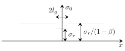
Figure 1: Distribution of piecewise constant initial yield stress $\sigma_{0}(x)$ of a uniform bar.

Under these assumptions, the initial yield stress distribution is given by

$$\sigma_{0}(x)=\left\{\begin{array}[]{l l}\sigma_{r}&\mbox{for }|x|<l_{g}\\ \sigma_{r}/(1-\beta)&\mbox{for }|x|>l_{g}\end{array}\right.$$ (23)

with discontinuities at $x=\pm l_{g}$, cf. Fig. 1. The response of the bar is elastic as long as the stress remains below the plastic limit, and the onset of yielding occurs when the yield limit is attained, i.e., when $F=F_{r}$ with $F_{r}=A\sigma_{r}=$ elastic limit force.

3.1 Plastic Zone Contained in Weak Segment

First, let us assume that the plastic zone $\mathcal{I}_{p}$ is fully contained in the weak segment, i.e. $\mathcal{I}_{p}\subset(-l_{g},l_{g})$. Then, the yield condition in Eq. (12), upon substitution of $A(x)=A_{c}$ and $EA(u^{\prime}-\kappa)=F=A_{c}\sigma_{c}$, is simplified to

$$l^{4}\kappa^{\mathrm{IV}}(x)-\kappa(x)=\frac{\sigma_{r}-\sigma_{c}}{H}\mbox{ for }x\in\mathcal{I}_{p}$$ (24)

which is a fourth-order linear differential equation with constant coefficients and a constant right-hand side. It will be convenient for further analysis to convert Eq. (24) into a normalized form. To this purpose, we introduce

• dimensionless spatial coordinate $\xi=x/l$,

• plastic strain at complete failure for the local model $\kappa_{f}=-\sigma_{r}/H$,

• normalized plastic strain $\kappa_{n}=\kappa/\kappa_{f}=-H\kappa/\sigma_{r}$,

• dimensionless stress or load parameter $\phi=F/F_{r}$,

• dimensionless parameters describing the ratio $\lambda_{g}=l_{g}/l$ between ”geometric” and material characteristic lengths, and

• ratio $\lambda_{p}=L_{p}/2l$ between one half of plastic zone and the material characteristic length.

In terms of normalized quantities, Eq. (24) is transformed into

$$\kappa_{n}^{\mathrm{IV}}(\xi)-\kappa_{n}(\xi)=\phi-1\mbox{ for }\xi\in(-\lambda_{p},\lambda_{p})$$ (25)

where, for simplicity, the derivatives with respect to $\xi$ are still denoted by primes or Latin numerals. The general solution to Eq. (25) is

$$\kappa_{n}(\xi)=C_{1}\cos{\xi}+C_{2}\sin{\xi}+C_{3}\cosh{\xi}+C_{4}\sinh{\xi}+1-\phi$$ (26)

where the integration constants $C_{2}$ and $C_{4}$ vanish due to the symmetry conditions $\kappa_{n}^{\prime}(0)=0,\kappa_{n}^{\prime\prime\prime}(0)=0$. The remaining unknowns are the integration constants $C_{1}$, $C_{3}$, and the size of the plastic zone $\lambda_{p}$, which are determined from the regularity conditions at the boundary of the plastic zone $\partial\mathcal{I}_{p}$,

$$\kappa_{n}(\lambda_{p})=0,\quad\kappa_{n}^{\prime}(\lambda_{p})=0,\quad\kappa_{n}^{\prime\prime}(\lambda_{p})=0$$ (27)

Substitution of the general solution (26) into the boundary conditions (27) leads to the set of three equations

$$C_{1}\cos{\lambda_{p}}+C_{3}\cosh{\lambda_{p}} =\phi-1$$ (28)

$$C_{1}\sin{\lambda_{p}} =C_{3}\sinh{\lambda_{p}}$$

$$C_{1}\cos{\lambda_{p}} =C_{3}\cosh{\lambda_{p}}$$

Elimination of $C_{1}$ and $C_{3}$ reduces the above system to a single nonlinear equation

$$\tan{\lambda_{p}}=\tanh{\lambda_{p}}$$ (29)

Solutions of this transcendental equation can be found numerically; let us denote them $\pm m_{i}\doteq 0,\pm 3.9266,\pm 7.0686,\dots,i\in\mathbb{N}_{0}$. Of course, only positive values are of physical interest. For given $i\in\mathbb{N}$, the integration constants can be evaluated from the first two equations of the system (28) as

$$C_{1} =\frac{\phi-1}{2\cos m_{i}}$$ (30)

$$C_{3} =\frac{\phi-1}{2\cosh m_{i}}$$

The most localized plastic strain profile is obtained for $i=1$, i.e., for $\lambda_{p}=m_{1}$. This is also the standard, non-variational solution of the localization problem for a bar with perfectly uniform properties presented by Jirásek and Rolshoven (2009b), Eq. (40).

Outside the plastic zone, condition (17) simplifies to

$$\sigma_{c}\leq\sigma_{r}\mbox{ or, equivalently, }\phi\leq 1$$ (31)

Analysis of the second variation, presented in detail in A, reveals that the most localized solution is stable (provided that the material parameters and bar length satisfy a certain condition), i.e. it corresponds to a local minimum of $\Pi$, while the solutions for $i\geq 2$ are unstable.

So far we have assumed that the weak segment is long enough, $2l_{g}>2lm_{1}$, and thus the stable localized solution is not affected by stronger parts of the bar. Nevertheless, if the weak segment is shorter, the analysis needs to be modified.

3.2 Plastic Zone Extending to Strong Segments

Let us proceed to the case when $L_{p}>2l_{g}$, i.e. $\lambda_{g}<m_{1}$. In this situation, Eq. (25) must be extended to the parts surrounding the weak segment:

$$\kappa_{n}^{\mathrm{IV}}(\xi)-\kappa_{n}(\xi) =\phi-1 -\lambda_{g}<\xi<\lambda_{g}$$ for (32)

$$\kappa_{n}^{\mathrm{IV}}(\xi)-\kappa_{n}(\xi) =\phi+\frac{1}{\beta-1} \lambda_{g}<|\xi|<\lambda_{p}$$ for

yielding the general solution

$$\kappa_{n}(\xi)=\left\{\begin{aligned} &C_{1}\cos{\xi}+C_{2}\sin{\xi}+C_{3}\cosh{\xi}+C_{4}\sinh{\xi}+1-\phi&\mbox{for }&&-\lambda_{g}<\xi<\lambda_{g}&\\ &C_{5}\cos{\xi}+C_{6}\sin{\xi}+C_{7}\cosh{\xi}+C_{8}\sinh{\xi}+\frac{1}{1-\beta}-\phi&\mbox{for }&&\lambda_{g}<\xi<\lambda_{p}&\\ &C_{9}\cos{\xi}+C_{10}\sin{\xi}+C_{11}\cosh{\xi}+C_{12}\sinh{\xi}+\frac{1}{1-\beta}-\phi&\mbox{for }&&-\lambda_{p}<\xi<\lambda_{g}&\end{aligned}\right.$$ (33)

By the symmetry conditions, the integration constants $C_{2}$ and $C_{4}$ vanish again, and

$$C_{5} =C_{9},$$ (34)

$$C_{6} =-C_{10},$$

$$C_{7} =C_{11},$$

$$C_{8} =-C_{12}$$

The remaining unknown constants $C_{i}$ for $i=1,3,5,6,7,8$ and the dimensionless plastic zone size $\lambda_{p}$ can be determined from seven conditions; namely from continuity of $\kappa$, $\kappa^{\prime}$, $HAl^{4}\kappa^{\prime\prime}$, and $(HAl^{4}\kappa^{\prime\prime})^{\prime}$ at $\xi=\lambda_{g}$, and of $\kappa$, $\kappa^{\prime}$, and $HAl^{4}\kappa^{\prime\prime}$ at $\xi=\lambda_{p}$. Because the resulting set of equations is nonlinear in $\lambda_{p}$, it is more convenient to solve the system for $C_{i}$ and $\phi$, with $\lambda_{p}$ considered as given. In other words, the loading process is considered as parametrized by $\lambda_{p}$ instead of $\phi$. Then, we arrive at a set of seven linear equations in the form

$$\left(\begin{array}[]{c c r r}-\cos{\lambda_{g}}&-\cosh{\lambda_{g}}&\cos{\lambda_{g}}&\sin{\lambda_{g}}\\ \sin{\lambda_{g}}&-\sinh{\lambda_{g}}&-\sin{\lambda_{g}}&\cos{\lambda_{g}}\\ -\cos{\lambda_{g}}&\cosh{\lambda_{g}}&\cos{\lambda_{g}}&\sin{\lambda_{g}}\\ \sin{\lambda_{g}}&\sinh{\lambda_{g}}&-\sin{\lambda_{g}}&\cos{\lambda_{g}}\\ 0&0&\cos{\lambda_{p}}&\sin{\lambda_{p}}\\ 0&0&-\sin{\lambda_{p}}&\cos{\lambda_{p}}\\ 0&0&\cos{\lambda_{p}}&\sin{\lambda_{p}}\end{array}\right.$$ (35)

$$\qquad\qquad\qquad\left.\begin{array}[]{r r c}\cosh{\lambda_{g}}&\sinh{\lambda_{g}}&0\\ \sinh{\lambda_{g}}&\cosh{\lambda_{g}}&0\\ -\cosh{\lambda_{g}}&-\sinh{\lambda_{g}}&0\\ -\sinh{\lambda_{g}}&-\cosh{\lambda_{g}}&0\\ \cosh{\lambda_{p}}&\sinh{\lambda_{p}}&-1\\ \sinh{\lambda_{p}}&\cosh{\lambda_{p}}&0\\ -\cosh{\lambda_{p}}&-\sinh{\lambda_{p}}&0\end{array}\right)\left(\begin{array}[]{c}C_{1}\\ C_{3}\\ C_{5}\\ C_{6}\\ C_{7}\\ C_{8}\\ \phi\end{array}\right)=\left(\begin{array}[]{c}\frac{\beta}{\beta-1}\\ 0\\ 0\\ 0\\ \frac{1}{\beta-1}\\ 0\\ 0\end{array}\right)$$

which can be easily solved by matrix inversion; for the sake of brevity, however, we do not provide the results in the explicit form. The resulting dependencies between the load parameter $\phi$ and normalized plastic zone $\lambda_{p}$ are depicted in Fig. 2 for several values of $\lambda_{g}=m_{1}\{0.003,0.025,0.127,0.255,0.382,0.637\}$ and for $\beta=0.5$.

Solving the system in Eq. (35) and substituting the results into Eq. (33) leads to the distribution of plastic strain $\kappa_{n}$. An example for $\lambda_{g}=0.127m_{1}$, $\beta=0.5$ and the monotonically expanding plastic zone $\lambda_{p}=m_{1}\{0.277,0.554,0.693,0.776,0.831,0.858,0.870\}$ is shown in Fig. 3a. In Fig. 3b, the third derivative of plastic strain is depicted, satisfying all the regularity requirements summarized in Tab. 1.

Integrating Eq. (33) over the length of the plastic zone provides the normalized plastic elongation

$$\frac{u_{p}}{l\kappa_{f}}=\int_{-\lambda_{p}}^{\lambda_{p}}\kappa_{n}(\xi)\,\mathrm{d}\xi=2\int_{0}^{\lambda_{g}}\kappa_{n}(\xi)\,\mathrm{d}\xi+2\int_{\lambda_{g}}^{\lambda_{p}}\kappa_{n}(\xi)\,\mathrm{d}\xi$$ (36)

which in this simple case can be carried out analytically:

$$\frac{u_{p}}{l\kappa_{f}}= \,2\bigg{\{}\frac{\beta\lambda_{g}+\lambda_{p}[\phi(1-\beta)-1]}{\beta-1}+C_{1}\sin{\lambda_{g}}+C_{3}\sinh{\lambda_{g}}+C_{5}(\sin{\lambda_{p}}-\sin{\lambda_{g}})$$ (37)

$$+C_{6}(\cos{\lambda_{g}}-\cos{\lambda_{p}})+C_{7}(\sinh{\lambda_{p}}-\sinh{\lambda_{g}})+C_{8}(\cosh{\lambda_{p}}-\cosh{\lambda_{g}})\bigg{\}}$$

The dimensionless load-plastic elongation diagrams for fixed $\beta=0.5$ and different dimensionless sizes of the weak segment $\lambda_{g}$ are shown in Fig. 4a, and for fixed $\lambda_{g}=0.127m_{1}$ with different values of $\beta$ in Fig. 4b. These figures reflect the influence of both parameters on the shape of the load-displacement curve for a bar with an imperfection, where $\lambda_{g}$ is understood as the length of the imperfection, and $\beta$ as its magnitude. Note that regardless of the imperfection shape and size, the plastic response of the bar is always of the same slope. For shorter imperfections we observe significant hardening, while for longer imperfections the response attains the behaviour of a perfectly uniform bar. The imperfection magnitude influences the load-displacement diagram in the opposite way; for large values of $\beta$, the response exhibits a higher maximum force. On the other hand, in the case of small magnitudes the response approaches the behaviour of a uniform bar discussed in Section 3.1. As an alternative physical interpretation, we could consider a semi-infinite layer of material between two parallel planes which are mutually displaced in tangential direction and left unconstrained in the normal direction, so that the layer with vertically variable material properties is under pure shear stress.

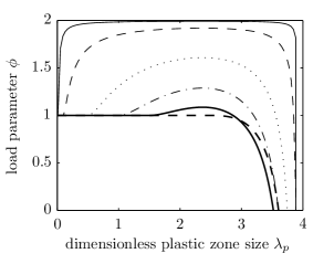
Figure 2: Piecewise constant yield stress distribution: relation between load parameter and plastic zone size for several values of $\lambda_{g}$, and for $\beta=0.5$; for complete legend please refer to Fig. 4a.

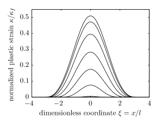
(a)

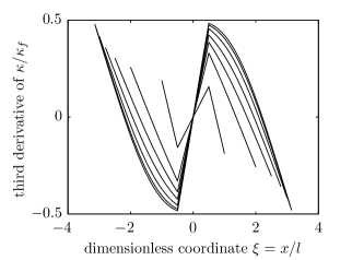
(b)

Figure 3: Piecewise constant yield stress distribution: (a) evolution of plastic strain profile and (b) its third derivative for monotonically increasing plastic zone length $\lambda_{p}$.

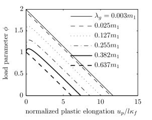
(a)

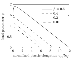
(b)

Figure 4: Piecewise constant yield stress distribution: (a) plastic part of dimensionless load-displacement diagram for different values of dimensionless imperfection length $\lambda_{g}$ assuming fixed $\beta=0.5$, and (b) for different values of dimensionless imperfection magnitude $\beta$ assuming fixed $\lambda_{g}=0.127m_{1}$.

In order to demonstrate that we have obtained an admissible solution, we check condition (17), which is valid outside the plastic zone and simplifies to

$$\phi\leq\frac{1}{1-\beta}$$ (38)

The condition can be simply verified in Fig. 2, where we have $\phi\leq 2$ for $\beta=0.5$.

Finally, in Fig. 5, we check that the energy balance (E) holds along the whole loading process in agrement with general results (Pham et al., 2011, Section 2.2.3) and (Pham and Marigo, 2013, Property 1) for solutions sufficiently regular in time. We observe that the response is first elastic, i.e. the $\mathcal{E}$ curve is quadratic with no dissipation $\mbox{Var}_{\mathcal{D}}$, followed by the evolution of the plastic strain accompanied by nonzero dissipation. For this graph, physical constants presented in Tab. 2 were used. Parameters that control the imperfection were set to $\lambda_{g}=0.255m_{1}$ and $\beta=0.5$, the total length of the bar was $L=4lm_{1}$, and the evolution was parametrized by the dimensionless plastic zone length

$$\lambda_{p}(t)=\lambda_{g}+t(m_{1}-\lambda_{g})\mbox{ for }t\in[0,1]$$ (39)

Table 2: Physical and geometric parameters of all test examples.

Physical parameters	Values
Young’s modulus, $E$	$60$	GPa
Softening modulus, $H$	$-10$	GPa
Characteristic length, $l$	$0$	$.05$ m
Reference initial yield stress, $\sigma_{r}$	$200$	MPa
Weakest cross-sectional area, $A_{c}$	$0$	$.01$ m2

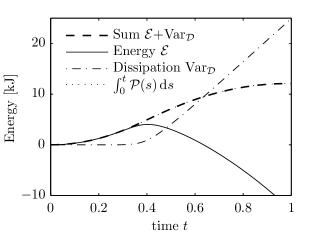
Figure 5: Piecewise constant yield stress distribution: energy evolution for $\beta=0.5$; see Tab. 2 for the physical parameters and Eq. (39) for the loading program.

4 Bar With Piecewise Constant Stress Distribution

In all subsequent sections, contrary to the previous one, we will assume the initial yield stress to be constant, i.e. $\sigma_{0}(x)=\sigma_{r}$, and will investigate the influence of the variable cross-sectional area resulting in spatially variable stress field distributions. As the first example, let us consider a very similar load test to that presented in Section 3, but now with discontinuous sectional area, i.e. a bar containing a thin segment of length $2l_{g}$ and sectional area $A_{c}$, and with remaining thick parts of sectional area $A_{c}/(1-\beta)$ where, as previously, $\beta\in(0,1)$ denotes a dimensionless parameter, cf. Fig. 6a.

The corresponding stress distribution is described by

$$\sigma(x)=\left\{\begin{array}[]{l l}F/A_{c}=\sigma_{c}&\mbox{for }|x|<l_{g}\\ F/[A_{c}/(1-\beta)]=(1-\beta)\sigma_{c}&\mbox{for }|x|>l_{g}\end{array}\right.$$ (40)

again with discontinuities at $x=\pm l_{g}$, cf. Fig. 7. Clearly, the case of a plastic zone contained in the weak segment coincides exactly with the situation presented in Section 3.1, and hence is not discussed again. Instead, let us proceed directly to the case in which $L_{p}>2l_{g}$, i.e., $\lambda_{g}\leq m_{1}$.

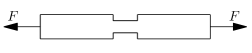
(a)

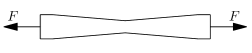
(b)

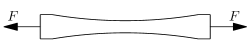
(c)

Figure 6: Geometries of tensile test bars corresponding to (a) discontinuous, (b) continuous, but not continuously differentiable, and (c) infinitely smooth stress fields.

Figure 7: Bar with piecewise constant cross-sectional area and the corresponding stress distribution.

4.1 Plastic Zone Extending to Thick Segments

Substituting Eq. (40) into the yield condition (12) and converting the result into the dimensionless form, we obtain the governing equations, cf. Eq. (32):

$$\kappa_{n}^{\mathrm{IV}}(\xi)-\kappa_{n}(\xi) =\phi-1 -\lambda_{g}<\xi<\lambda_{g}$$ for (41)

$$\kappa_{n}^{\mathrm{IV}}(\xi)-\kappa_{n}(\xi) =\phi-\beta\phi-1 \lambda_{g}<|\xi|<\lambda_{p}$$ for

which provide the general solution

$$\kappa_{n}(\xi)=\left\{\begin{aligned} &C_{1}\cos{\xi}+C_{2}\sin{\xi}+C_{3}\cosh{\xi}+C_{4}\sinh{\xi}+1-\phi&\mbox{for }&&-\lambda_{g}<\xi<\lambda_{g}&\\ &C_{5}\cos{\xi}+C_{6}\sin{\xi}+C_{7}\cosh{\xi}+C_{8}\sinh{\xi}+1-\phi+\beta\phi&\mbox{for }&&\lambda_{g}<\xi<\lambda_{p}&\\ &C_{9}\cos{\xi}+C_{10}\sin{\xi}+C_{11}\cosh{\xi}+C_{12}\sinh{\xi}+1-\phi+\beta\phi&\mbox{for }&&-\lambda_{p}<\xi<\lambda_{g}&\end{aligned}\right.$$ (42)

By the symmetry arguments, the integration constants $C_{2}$ and $C_{4}$ are zero, and for $C_{i}$, $i=9,\dots,12$, the relations (34) hold again. The remaining unknown constants $C_{i}$ for $i=1,3,5,6,7,8$ and the dimensionless plastic zone size $\lambda_{p}$ can be determined from the regularity conditions; for example, continuity of $HAl^{4}\kappa^{\prime\prime}$ and $(HAl^{4}\kappa^{\prime\prime})^{\prime}$ at $\xi=\lambda_{g}$ give

$$(1-\beta)\kappa_{n}^{\prime\prime}(\lambda_{g}^{-}) =\kappa_{n}^{\prime\prime}(\lambda_{g}^{+})$$ (43)

$$(1-\beta)\kappa_{n}^{\prime\prime\prime}(\lambda_{g}^{-}) =\kappa_{n}^{\prime\prime\prime}(\lambda_{g}^{+})$$

The set of seven linear equations arising from the regularity and boundary conditions reads

$$\left(\begin{array}[]{c c r r}-\cos{\lambda_{g}}&-\cosh{\lambda_{g}}&\cos{\lambda_{g}}&\sin{\lambda_{g}}\\ \sin{\lambda_{g}}&-\sinh{\lambda_{g}}&-\sin{\lambda_{g}}&\cos{\lambda_{g}}\\ (\beta-1)\cos{\lambda_{g}}&(1-\beta)\cosh{\lambda_{g}}&\cos{\lambda_{g}}&\sin{\lambda_{g}}\\ (1-\beta)\sin{\lambda_{g}}&(1-\beta)\sinh{\lambda_{g}}&-\sin{\lambda_{g}}&\cos{\lambda_{g}}\\ 0&0&\cos{\lambda_{p}}&\sin{\lambda_{p}}\\ 0&0&-\sin{\lambda_{p}}&\cos{\lambda_{p}}\\ 0&0&\cos{\lambda_{p}}&\sin{\lambda_{p}}\end{array}\right.$$ (44)

$$\qquad\qquad\qquad\left.\begin{array}[]{r r c}\cosh{\lambda_{g}}&\sinh{\lambda_{g}}&\beta\\ \sinh{\lambda_{g}}&\cosh{\lambda_{g}}&0\\ -\cosh{\lambda_{g}}&-\sinh{\lambda_{g}}&0\\ -\sinh{\lambda_{g}}&-\cosh{\lambda_{g}}&0\\ \cosh{\lambda_{p}}&\sinh{\lambda_{p}}&\beta-1\\ \sinh{\lambda_{p}}&\cosh{\lambda_{p}}&0\\ -\cosh{\lambda_{p}}&-\sinh{\lambda_{p}}&0\end{array}\right)\left(\begin{array}[]{c}C_{1}\\ C_{3}\\ C_{5}\\ C_{6}\\ C_{7}\\ C_{8}\\ \phi\end{array}\right)=\left(\begin{array}[]{c}0\\ 0\\ 0\\ 0\\ -1\\ 0\\ 0\end{array}\right)$$

and for convenience it is again solved numerically with no explicit expressions presented. The resulting dependencies between the load parameter $\phi$ and the normalized plastic zone size $\lambda_{p}$ are depicted in Fig. 8 for the same values $\lambda_{g}$ and $\beta$ as in Section 3.2, see also Fig. 2.

The normalized plastic strain, analytically expressed in Eq. (42), is depicted in Fig. 9a for $\lambda_{g}=0.127m_{1}$, $\beta=0.5$, and for a monotonically expanding plastic zone $\lambda_{p}=m_{1}\{0.277,0.554,0.693,0.776,0.831,0.858,0.870\}$. Its third derivative, presented in Fig. 9b, exhibits discontinuities at $\xi=\pm\lambda_{g}$ and $\xi=\pm\lambda_{p}$. Let us note, however, that the quantity $A(\xi)\kappa_{n}^{\prime\prime\prime}(\xi)$ plotted in Fig. 10b has non-negative jumps only at $\xi=\pm\lambda_{p}$ and remains continuous for $\xi\in(-\lambda_{p},\lambda_{p})$ in accordance to the discussion presented at the end of Section 2.1. For completeness, continuity of $A(\xi)\kappa_{n}^{\prime\prime}(\xi)$ and validity of plastic yield condition (12) or plastic admissibility condition (13) can be verified in Figs. 10a and 11.

The normalized plastic elongation, with the general expression presented in Eq. (36), can be again evaluated analytically:

$$\frac{u_{p}}{l\kappa_{f}}= \,2\big{\{}\lambda_{p}[1+\phi(\beta-1)]-\phi\beta\lambda_{g}+C_{1}\sin{\lambda_{g}}+C_{3}\sinh{\lambda_{g}}+C_{5}(\sin{\lambda_{p}}-\sin{\lambda_{g}})$$ (45)

$$+C_{6}(\cos{\lambda_{g}}-\cos{\lambda_{p}})+C_{7}(\sinh{\lambda_{p}}-\sinh{\lambda_{g}})+C_{8}(\cosh{\lambda_{p}}-\cosh{\lambda_{g}})\big{\}}$$

Dimensionless load-plastic elongation diagrams for fixed $\beta=0.5$ and for different dimensionless sizes of the thin segment $\lambda_{g}$ are presented in Fig. 12a; the influence of $\beta$ for fixed $\lambda_{g}=0.127m_{1}$ with different values of $\beta$ is shown in Fig. 12b. Notice that the obtained results resemble those presented in Section 3.2 for a bar with piecewise constant initial yield stress. However, the slope of the load-displacement diagram now strongly depends on $\lambda_{g}$ and $\beta$.

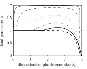
Figure 8: Piecewise constant stress distribution: relation between load parameter and plastic zone size for several values of $\lambda_{g}$, and for $\beta=0.5$; for complete legend please refer to Fig. 12a.

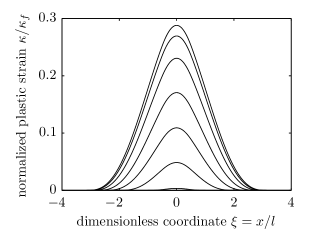
(a)

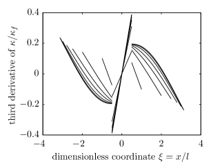
(b)

Figure 9: Piecewise constant stress distribution: (a) evolution of plastic strain profile and (b) its third derivative for monotonically increasing plastic zone length $\lambda_{p}$.

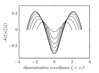
(a)

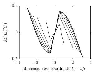
(b)

Figure 10: Piecewise constant stress distribution: (a) evolution of $A(\xi)\kappa_{n}^{\prime\prime}(\xi)$ and (b) $A(\xi)\kappa_{n}^{\prime\prime\prime}(\xi)$ for monotonically increasing plastic zone length $\lambda_{p}$, and for fixed $\lambda_{g}=0.127m_{1}$, $\beta=0.5$.

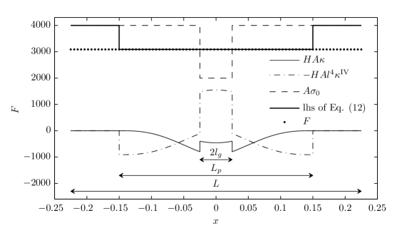
Figure 11: Piecewise constant stress distribution: a pictorial demonstration of plastic yield condition (12) valid in $\mathcal{I}_{p}$, and plastic admissibility condition (13) valid in $\mathcal{I}_{e}$ for $\lambda_{g}=0.127m_{1}$, $\lambda_{p}=0.762m_{1}$, $\beta=0.5$, and $\frac{L}{2l}=1.5\lambda_{p}$.

(a)

(b)

Figure 12: Piecewise constant stress distribution: (a) plastic part of dimensionless load-displacement diagram for different values of dimensionless length $\lambda_{g}$ assuming fixed $\beta=0.5$, and (b) for different values of $\beta$ assuming fixed $\lambda_{g}=0.127m_{1}$.

Plastic admissibility condition (17) valid outside the plastic zone provides the inequality already presented in Eq. (38), and can be simply verified in Fig. 8, where for $\beta=0.5$ we require $\phi\leq 2$.

Finally, the energy profiles corresponding to the loading program (39) are depicted in Fig. 13, where we can check that the solution satisfies the energy balance (E) along the whole loading path. Physical constants are summarized in Tab. 2; the parameters reflecting the size of the thin segment were set to $\lambda_{g}=0.255m_{1}$ and $\beta=0.5$, and the total length of the bar was $L=4lm_{1}$.

Figure 13: Piecewise constant stress distribution: energy evolution for $\beta=0.5$; see Tab. 2 for the physical parameters and Eq. (39) for the loading program.

5 Bar With Piecewise Linear Stress Distribution

Now we proceed to a bar with a continuous but not continuously differentiable stress distribution, cf. Fig. 6b. The cross-sectional area corresponding to a piecewise linear stress distribution is specified in the form

$$A(x)=\frac{A_{c}l_{g}}{l_{g}-|x|}$$ (46)

where the overall length of the bar $L=2l_{g}$ now represents the supremum over all possible bar lengths for which the example is meaningful; note that $\lim_{x\rightarrow\pm l_{g}}A(x)=+\infty$. As in the previous section, $A_{c}$ denotes the area of the weakest cross section. Substituting $A(x)$ into Eq. (12) with $\sigma_{0}(x)=\sigma_{r}$, we obtain

$$l^{4}\left[\kappa^{\mathrm{IV}}(x)+\frac{2\,\mbox{sgn}(x)}{l_{g}-|x|}\kappa^{\prime\prime\prime}(x)+\frac{2}{(l_{g}-|x|)^{2}}\kappa^{\prime\prime}(x)\right]-\kappa(x)=\frac{\sigma_{r}}{H}-\frac{\sigma_{c}}{Hl_{g}}(l_{g}-|x|)\mbox{ for }x\in\mathcal{I}_{p}\backslash\{0\}$$ (47)

which has to be satisfied at all points inside the plastic zone with the exception of $x=0$, where the cross-sectional area is not differentiable. At that point, we enforce continuity conditions of $\kappa$, $\kappa^{\prime}$, $A\kappa^{\prime\prime}$ and $(A\kappa^{\prime\prime})^{\prime}$, recall the discussion at the end of Section 2.1 and Tab. 1. Since $A$ is continuous, the third condition actually reduces to continuity of $\kappa^{\prime\prime}$. After conversion to the dimensionless form, in Section 3.1, the governing equation transforms into

$$\kappa_{n}^{\mathrm{IV}}(\xi)+\frac{2\,\mbox{sgn}(\xi)}{\lambda_{g}-|\xi|}\kappa_{n}^{\prime\prime\prime}(\xi)+\frac{2}{(\lambda_{g}-|\xi|)^{2}}\kappa_{n}^{\prime\prime}(\xi)-\kappa_{n}(\xi)=\phi-1-\phi\frac{|\xi|}{\lambda_{g}}\mbox{ for }\xi\in(-\lambda_{p},\lambda_{p})\backslash\{0\}$$ (48)

This is a fourth-order differential equation, and contrary to Eqs. (25), (32), and (41), it has non-constant coefficients and a non-constant right-hand side term. Although an analytical solution can be constructed in terms of special functions—the coefficients of the homogeneous part of equation (48) fulfil the so-called Calabi-Yau condition, cf. Almkvist et al. (2011), Eq. (3.4)—it is more convenient to solve it using the MATLAB^® bvp4c solver, for details see Shampine et al. (2003). Again, due to symmetry conditions, it suffices to restrict our attention to the positive part of the plastic zone, $\mathcal{I}_{p}^{+}=(0,\lambda_{p})$. Then, the boundary and symmetry conditions read

$$\kappa_{n}(\lambda_{p})=0,\kappa_{n}^{\prime}(\lambda_{p})=0,\kappa_{n}^{\prime\prime}(\lambda_{p})=0,\mbox{ and }$$ (49)

$$\kappa_{n}^{\prime}(0)=0,\kappa_{n}^{\prime\prime\prime}(0^{+})=-\kappa_{n}^{\prime\prime}(0)/\lambda_{g}$$

The last condition is obtained from continuity of $(A\kappa^{\prime\prime})^{\prime}$, meaning that $(A\kappa^{\prime\prime})^{\prime}(0^{-})=(A\kappa^{\prime\prime})^{\prime}(0^{+})$, and can be derived when taking into account continuity of $A$, $\kappa^{\prime\prime}$ and skew-symmetry of $A^{\prime}$, $\kappa^{\prime\prime\prime}$, i.e. $A^{\prime}(0^{-})=-A^{\prime}(0^{+})$, $\kappa^{\prime\prime\prime}(0^{-})=-\kappa^{\prime\prime\prime}(0^{+})$. The solution is again parametrized by the length of the plastic zone $\lambda_{p}$, and for each $\lambda_{p}$ the corresponding $\phi$ is determined from the solution of (48) and (49).

Before presenting the obtained results, let us briefly comment on the numerical solutions. Since the bvp4c solver is employed to provide only the continuous part of the solution on $\mathcal{I}_{p}^{+}$, the jump condition becomes a boundary condition that is imposed directly. Moreover, the solver relies on a collocation method for iterative solution of boundary value problems with nonlinear two-point boundary conditions, and it is therefore robust with respect to possible changes of input data compared e.g. to shooting-based strategies used in Jirásek and Zeman (2015). For further details, we refer to Shampine et al. (2003), Section 3.

The plastic part of the load-displacement diagram is depicted in Fig. 14a, where the dimensionless load parameter $\phi$ is plotted against the dimensionless plastic elongation $u_{p}/l\kappa_{f}$. The initial part of the diagram is vertical, as in the previous examples, since only the elastic deformation evolves for $F<F_{r}$. At the onset of yielding, the load parameter first steeply increases and only later decreases. Complete failure is attained at larger elongation in comparison with the non-variational formulation analyzed in Jirásek et al. (2010). Several values $\lambda_{g}=\{1.019,2.037,4.075,8.150\}m_{1}$ are reported (from top to bottom), to reflect the effect of spatial variation of the sectional area; lower values of $\lambda_{g}$ correspond to a stronger variation of the sectional area and lead to higher peak loads. Note that for the standard formulation, the overall elongation at failure is always the same, while for the variational approach it depends on $\lambda_{g}$.

Fig. 14b captures the evolution of the plastic zone size. The load parameter $\phi$ is plotted against the dimensionless plastic zone size $\lambda_{p}$, obtained again for several values of $\lambda_{g}$. We can infer from the figure that the plastic zone evolves continuously and monotonically from the weakest section to its full size. The length at complete failure is almost the same as for the standard solution, plotted by dashed curves.

The evolution of the plastic strain profile and of its third spatial derivative is depicted in Fig. 15 for $\lambda_{g}=1.019m_{1}$ and several values of $\lambda_{p}=m_{1}\{0.255,0.637,0.764,0.891,0.998\}$. First, during the early stages of plastic evolution, the standard and variational solutions are almost the same, but at later stages, the differences grow significantly. Contrary to the standard solution, $\kappa^{\prime\prime\prime}$ is discontinuous for the variational solution at $\xi=0$, where $\llbracket\kappa^{\prime\prime\prime}\rrbracket_{0}=-2\kappa^{\prime\prime}(0)/l_{g}$.

(a)

(b)

Figure 14: Piecewise linear stress distribution: (a) plastic part of load-displacement diagram, and (b) relation between load parameter and plastic zone for $\lambda_{g}=\{1.019,2.037,4.075,8.150\}m_{1}$. The maximum value of the load parameter $\phi$ decreases with increasing $\lambda_{g}$.

(a)

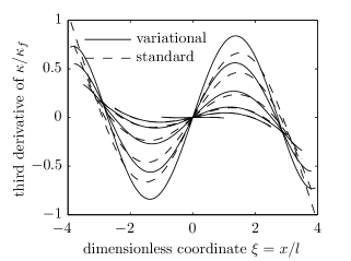
(b)

Figure 15: Piecewise linear stress distribution: (a) evolution of plastic strain profile and (b) third derivative of plastic strain for monotonically increasing plastic zone length $\lambda_{p}$.

(a) standard

(b) variational

Figure 16: Piecewise linear stress distribution: energy evolutions; see Tab. 2 for the physical parameters and Eq. (52) for the loading program.

In the elastic zone $\mathcal{I}_{e}$, condition (17) for an admissible solution reduces to

$$\phi\leq\frac{1}{1-\frac{\xi}{\lambda_{g}}}$$ (50)

where it is sufficient to verify $\xi=\lambda_{p}$. For the data in Fig. 14b we obtain

$$\phi\leq\frac{1}{1-\frac{1}{4}}=\frac{4}{3}$$ (51)

and the condition is satisfied. For $\lambda_{p}\rightarrow\lambda_{g}$, however, the right-hand side in (50) converges to $+\infty$ showing that plastification of points close to physical boundary $\partial\Omega$ would require a very strong growth of $\phi$.

Figure 16 depicts the energy balance (E) for the standard solution (Fig. 16a) and for the energetic solution (Fig. 16b) obtained for the data presented in Tab. 2. Further, we have used $\lambda_{g}=1.02m_{1}$ and have parametrized the localization process through

$$\lambda_{p}(t)=m_{1}t\mbox{ for }t\in[0,1]$$ (52)

It is worth noting that, for the standard solution, the work done by external forces $\int_{0}^{t}\mathcal{P}(s)\,\mathrm{d}s$ is out of balance with $\mathcal{E}+\mathrm{Var}_{\mathcal{D}}$, while the variational approach delivers an energy-conserving process.

6 Bar With Quadratic Stress Distribution

As the final example, we shall present the most regular case of quadratic stress distribution possessing continuous derivatives of an arbitrary order, see Fig. 6c. The function describing the cross-sectional area then reads

$$A(x)=\frac{A_{c}l_{g}^{2}}{l_{g}^{2}-x^{2}}$$ (53)

where the overall length of the bar $L=2l_{g}$ is, in analogy to Eq. (46), understood as the supremum over all possible bar lengths for which the example is meaningful; note that again, $\lim_{x\rightarrow\pm l_{g}}A(x)=+\infty$. Upon substitution into the yield condition (12) with $\sigma_{0}(x)=\sigma_{r}$, we get the governing equation

$$l^{4}\left[\kappa^{\mathrm{IV}}(x)+\frac{4x}{l_{g}^{2}-x^{2}}\kappa^{\prime\prime\prime}(x)+\frac{2(l_{g}^{2}+3x^{2})}{(l_{g}^{2}-x^{2})^{2}}\kappa^{\prime\prime}(x)\right]-\kappa(x)=\frac{\sigma_{r}}{H}-\frac{\sigma_{c}}{H}\left(1-\frac{x^{2}}{l_{g}^{2}}\right)\mbox{ for }x\in\mathcal{I}_{p}$$ (54)

which can be converted into the dimensionless form

$$\kappa_{n}^{\mathrm{IV}}(\xi)+\frac{4\xi}{\lambda_{g}^{2}-\xi^{2}}\kappa_{n}^{\prime\prime\prime}(\xi)+\frac{2(\lambda_{g}^{2}+3\xi^{2})}{(\lambda_{g}^{2}-\xi^{2})^{2}}\kappa_{n}^{\prime\prime}(\xi)-\kappa_{n}(\xi)=\phi-1-\phi\frac{\xi^{2}}{\lambda_{g}^{2}}\mbox{ for }\xi\in(-\lambda_{p},\lambda_{p})$$ (55)

As in the previous case, we will employ a numerical solver, since the governing equation is even more complicated. Owing to symmetry requirements, the solution will again be constructed in the positive half of the plastic zone $\mathcal{I}_{p}^{+}$, with boundary and symmetry conditions

$$\kappa_{n}(\lambda_{p})=0,\kappa_{n}^{\prime}(\lambda_{p})=0,\kappa_{n}^{\prime\prime}(\lambda_{p})=0$$ (56)

$$\kappa_{n}^{\prime}(0)=0,\kappa_{n}^{\prime\prime\prime}(0)=0$$

In contrast to (49), the last condition is now simpler since $A^{\prime}$ is continuous.

The solution has been computed for several values of $\lambda_{p}$. In Fig. 17a we notice that the plastic zone evolves continuously and monotonically; particular plastic strain profiles together with their third derivatives are depicted in Fig. 18 for $\lambda_{g}=1.273m_{1}$ and $\lambda_{p}=m_{1}\{0.255,0.636,0.764,0.891,0.968,0.998\}$. Comparing the results presented in Fig. 15 with the results in Fig. 18, we notice that for the quadratic stress distribution the differences between the standard and variational solutions are less pronounced. Due to a higher smoothness of the solution, the load-displacement diagram presented in Fig. 17b is almost linear, only with a slight hardening followed by the softening branch. Differences between plastic displacements at failure, i.e. for $\phi=0$, are also somewhat less distinct.

Hardening effects for the variational formulation are systematically stronger in comparison to the standard formulation; moreover, for small values of $\lambda_{g}$, the differences are more obvious. This effect has already been explained in Section 2.1, see Eq. (12), Tab. 1 and the discussion therein. Recall, nevertheless, that the two formulations differ in two terms with higher-order derivatives of the sectional area, neglected for the standard formulation. For decreasing magnitudes of $A^{\prime}(x)$ and $A^{\prime\prime}(x)$, the variational formulation approaches the standard one; the limit case is presented in Section 3.1, where the two solutions coincide. Let us note that for an infinitely differentiable exponential stress distribution, considered in Jirásek et al. (2013), we would also obtain significant differences for $\lambda_{g}$ small enough.

Substituting expression (53) into inequality (17) leads to

$$\phi\leq\frac{1}{1-\left(\frac{\xi}{\lambda_{g}}\right)^{2}}$$ (57)

which should hold inside $\mathcal{I}_{e}$, i.e. for all $|\xi|\geq\lambda_{p}$. A closer inspection of Fig. 17a reveals that the condition is satisfied.

Energy balances for the standard and variational formulations are shown in Fig. 19 using the data from Tab. 2 and loading program in Eq. (52). The total length of the bar was $2\lambda_{g}$ with $\lambda_{g}=1.019m_{1}$. Again, for the standard formulation we notice a slight violation of condition (E).

(a)

(b)

Figure 17: Quadratic stress distribution: (a) relation between load parameter and plastic zone size, (b) plastic part of load-displacement diagram for $\lambda_{g}=\{1.019,1.273,2.547,12.734\}m_{1}$. The maximum value of the load parameter $\phi$ decreases with increasing $\lambda_{g}$.

(a)

(b)

Figure 18: Quadratic stress distribution: (a) evolution of plastic strain profile and (b) third derivative of plastic strain for increasing $\lambda_{p}$.

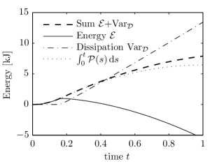
(a) standard

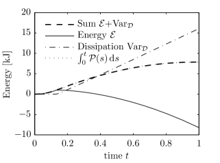
(b) variational

Figure 19: Quadratic stress distribution: energy evolutions; see Tab. 2 for the physical parameters and Eq. (52) for the loading program.

7 Summary and Conclusions

We have presented one-dimensional localization analysis of a softening plasticity model regularized by a variational formulation with a fourth-order gradient enrichment. The main results are summarized as follows:

1. Using a consistent variational approach, we have derived the description of a one-dimensional gradient plasticity model which provides not only the appropriate differential equation, representing the yield condition inside the plastic zone, but also appropriate forms of boundary and jump conditions at the elasto-plastic interface.

2. On the basis of the derived conditions that follow from the variational principle, two problems with discontinuous data (a bar or layer with discontinuous yield stress and a bar with discontinuous cross-sectional area) have been investigated. These examples are amenable to analytical solution and have provided physically reasonable results.

3. Two additional examples have been analysed, one with continuous but not continuously differentiable data and the other with smooth data. Numerical solutions have been constructed and compared to the alternative non-variational formulation, demonstrating that the variationally consistent formulation leads to higher peak loads and elongations at structural failure.

4. We have also investigated the influence of various data on the evolution of the plastic zone and on load-displacement diagrams for all four prototype problems. It has been shown that the plastic zone monotonically expands from the weakest section of the bar. In spite of the softening character of the material model, the structural response exhibits first hardening after the onset of yielding, later followed by softening. Such a behaviour is related to a gradual expansion of the plastic zone to stronger segments of the bar.

5. Further, it has been demonstrated that the solution corresponding to the variational formulation satisfies the energy balance along the evolution path of the localization process. Contrary to that, the standard formulation exhibits systematic lack of balance in the sense that the sum of elastic and dissipated energies exceeds the work done by external forces. In all cases, however, the dissipated energy remains finite and non-zero.

6. The variational approach is based on the non-negative first variation of the functional. Solutions corresponding to local minima of the functional have to satisfy this condition and moreover have to be stable. Hence, an analysis of the second variation providing some explicit requirements on physical constants is presented in A for the simplest case of a bar with perfectly uniform data.

Let us note that although we have not employed variable elastic or plastic moduli, the variational approach is perfectly suited to handle problems with discontinuities in such data.

The presented framework can also be extended to higher dimensions using e.g. the von Mises yield function with isotropic softening. Then, the free boundary conditions for the scalar cumulative plastic strain at the elastoplastic interface are analogous to those for $\kappa$ for sufficiently smooth fields only. However, in the multi-dimensional setting the required regularity is difficult to establish since, for instance, the embeddings $W^{1,2}\subset C^{0}$ or $W^{2,2}\subset C^{1}$ no longer hold; its rigorous investigation is beyond the scope of the present work.

Appendix A Second Variation and Stability Conditions

The analysis presented in the main part of the paper has been based on the condition of non-negative first variation of the energy functional $\Pi$. This condition is, however, only a necessary one, yet is not sufficient to ensure that the solution is a local minimum, thus that it is energetically stable. Therefore, in this section we discuss the behaviour of the energy functional in the vicinity of a solution $(u,\kappa)$ satisfying (11)–(13), drawing inspiration from a related analysis by Jirásek et al. (2013).

In particular, we will investigate the second variation of the energy functional given by Eq. (7). Our objective is to show that the second variation is positive for all those nonzero admissible variations $\delta u$ and $\delta\kappa$ for which the first variation $\delta\Pi$ vanishes, to ensure that the solution $(u,\kappa)$ is stable. Overall procedure will be described in six steps for better clarity. In A.1, we start with the elimination of the displacement field from the functional $\Pi$ in order to simplify stability conditions discussed in A.2, where the corresponding eigenvalue problem will be derived. In A.3 and A.4, we discuss even and odd eigenfunctions and specify the requirements on physical and geometric parameters leading to stable responses. A discussion of larger plastic zones for a uniform bar is presented in A.5. In A.6, we summarize our developments and briefly comment on problems with non-uniform cross-section area.

A.1 Condensation of Displacement Field

In the first step, we can simplify the problem by eliminating the displacement field and constructing a reduced functional that depends on the plastic strain field only. Indeed, the original functional (7) can first be minimized with respect to the displacements at fixed plastic strains. Integrating the already derived optimality condition (11) and assuming vanishing body forces $b$, we obtain

$$u^{\prime}(x)=\frac{F}{EA(x)}+\kappa(x)$$ (58)

where $F$ is the integration constant, physically corresponding to the axial force, cf. Eq. (22). Integrating again and taking into account the boundary conditions implied by (2a), we can express the normal force as

$$F=K_{e}\left(\overline{u}-\int_{\Omega}\kappa(x)\,\mbox{d}x\right)$$ (59)

where $\overline{u}(t)=u_{D}(\partial\Omega_{R},t)-u_{D}(\partial\Omega_{L},t)$ is the prescribed total elongation, and

$$K_{e}=\frac{1}{\displaystyle\int_{\Omega}\frac{\mbox{d}x}{EA(x)}}$$ (60)

is the elastic stiffness of the bar (reciprocal value of the elastic compliance). Based on (58)–(59) and on the assumption of no body forces ($b=0$), the original functional (7) can be reduced to

$$\Pi^{*}(\widehat{\kappa})=\frac{K_{e}}{2}\left(\overline{u}-\int_{\Omega}\widehat{\kappa}\,\mbox{d}x\right)^{2}+\frac{1}{2}\int_{\Omega}HA(\widehat{\kappa}^{2}-l^{4}\widehat{\kappa}^{\prime\prime 2})\,\mbox{d}x+\int_{\Omega}A\sigma_{0}\widehat{\kappa}\,\mbox{d}x$$ (61)

Note that the first term represents the elastically stored energy, expressed as a functional dependent on the plastic strain only. The expression in the parentheses is the elastic elongation, written as the difference between the total elongation $\overline{u}$ and the plastic part of elongation $u_{p}$ which was introduced in (36).

A.2 Second Variation

The first variation of the reduced functional $\Pi^{*}$ is given by

$$\delta\Pi^{*}({\kappa};\delta\kappa)=-K_{e}\left(\overline{u}-\int_{\Omega}{\kappa}\,\mbox{d}x\right)\int_{\Omega}\delta\kappa\,\mbox{d}x+\int_{\Omega}HA(\kappa\,\delta\kappa-l^{4}\kappa^{\prime\prime}\delta\kappa^{\prime\prime})\,\mbox{d}x+\int_{\Omega}A\sigma_{0}\delta\kappa\,\mbox{d}x$$ (62)

which exactly corresponds to (8) with $u^{\prime}$ and $\delta u^{\prime}$ expressed according to (58)–(59) and $b$ set to zero. The second variation of the reduced functional $\Pi^{*}$ is given by

$$\delta^{2}\Pi^{*}(\delta\kappa)=K_{e}\left(\int_{\Omega}\delta\kappa\,\mbox{d}x\right)^{2}+\int_{\Omega}HA(\delta\kappa^{2}-l^{4}\delta\kappa^{\prime\prime 2})\,\mbox{d}x$$ (63)

and is independent of $\kappa$ because $\Pi^{*}$ is quadratic.

We would now like to prove that the quadratic form $\delta^{2}\Pi^{*}$ is positive definite in the space of all those admissible variations $\delta\kappa$ for which $\delta\Pi^{*}(\kappa;\delta\kappa)=0$. Note that $\kappa$ is not arbitrary but represents the solution of the problem described by conditions (14)–(16), which were derived from the requirement $\delta\Pi(u,\kappa;\delta u,\delta\kappa)\geq 0$ for all admissible variations $\delta u$ and $\delta\kappa$ (and which could alternatively be derived, in a slightly different format, from the condition $\delta\Pi^{*}(\kappa;\delta\kappa)\geq 0$ for all admissible variations $\delta\kappa$). Integrating the term with $\delta\kappa^{\prime\prime}$ in (62) twice by parts and exploiting the properties of function $\kappa$ (in particular, the fact that $\kappa=0$ in $\mathcal{I}_{e}$), we can rewrite the first variation of $\Pi^{*}$ as

$$\delta\Pi^{*}({\kappa};\delta\kappa) = \int_{\mathcal{I}_{p}}\left[HA\kappa-(HAl^{4}\kappa^{\prime\prime})^{\prime\prime}+A\sigma_{0}-K_{e}\left(\overline{u}-\int_{\mathcal{I}_{p}}{\kappa}\,\mbox{d}x\right)\right]\delta\kappa\,\mbox{d}x$$ (64)

$$+\int_{\mathcal{I}_{e}}\left[A\sigma_{0}-K_{e}\left(\overline{u}-\int_{\mathcal{I}_{p}}{\kappa}\,\mbox{d}x\right)\right]\delta\kappa\,\mbox{d}x$$

$$-\sum_{\partial\mathcal{I}_{ep}}HAl^{4}\kappa^{\prime\prime}n\delta\kappa^{\prime}+\sum_{\partial\mathcal{I}_{ep}}(HAl^{4}\kappa^{\prime\prime})^{\prime}n\delta\kappa$$

where $n$ denotes the outer normal to $\mathcal{I}_{p}$. Taking into account that $\kappa$ satisfies the yield condition (12) in which the right-hand side corresponds to the normal force $F$, which is in turn equal to the expression given in (59), we can show that the expression in square brackets in the first integral in (64) vanishes. The first sum in (64) also vanishes because $\kappa^{\prime\prime}=0$ on $\partial\mathcal{I}_{ep}$. Consequently, (64) reduces to

$$\delta\Pi^{*}({\kappa};\delta\kappa)=\int_{\mathcal{I}_{e}}\left[A\sigma_{0}-K_{e}\left(\overline{u}-\int_{\mathcal{I}_{p}}{\kappa}\,\mbox{d}x\right)\right]\delta\kappa\,\mbox{d}x+\sum_{\partial\mathcal{I}_{ep}}(HAl^{4}\kappa^{\prime\prime})^{\prime}n\delta\kappa$$ (65)

Let us also recall that (i) the variation $\delta\kappa$ is nonnegative in $\mathcal{I}_{e}\cup\partial\mathcal{I}_{ep}$; (ii) the expression in the square brackets in (65) is nonnegative in $\mathcal{I}_{e}$, see condition (17); and (iii) the product $(HAl^{4}\kappa^{\prime\prime})^{\prime}n$ is nonnegative on $\partial\mathcal{I}_{ep}$, see the last line in Table 1. To proceed further, we need to assume that the expression in the square brackets in (65) is strictly positive (not just nonnegative) in $\mathcal{I}_{e}$. This assumption means that the normal force in the entire elastic domain is below the yield limit, which is true for all the localized solutions presented in this paper. Consequently, for those admissible variations $\delta\kappa$ that are not identically zero in $\mathcal{I}_{e}$, the integral in (65) is positive and thus the first variation $\delta\Pi^{*}$ is positive, because the second term on the right-hand side of (65) is always nonnegative.

Based on the foregoing analysis of the first variation, we can see that positive definiteness of the second variation $\delta^{2}\Pi^{*}$ needs to be proven for those variations $\delta\kappa$ that vanish in $\mathcal{I}_{e}$, and the integration domains in (63) can be restricted to $\mathcal{I}_{p}$. To preserve continuous differentiability of $\delta\kappa$ in $\Omega$, its value and first derivative on $\partial\mathcal{I}_{ep}\equiv\partial\mathcal{I}_{p}$ must be zero. To simplify notation, we will use from now on $v$ instead of $\delta\kappa$. The stability condition is then satisfied if there exists some $\alpha>0$ such that

$$K_{e}\left(\int_{\mathcal{I}_{p}}v\,\mbox{d}x\right)^{2}+\int_{\mathcal{I}_{p}}HA(v^{2}-l^{4}v^{\prime\prime 2})\,\mbox{d}x\geq\alpha\|v\|^{2}\hskip 14.22636pt\mbox{for all }v\in\mathcal{V}$$ (66)

where

$$\mathcal{V}=\widetilde{W}^{2,2}_{0}(\mathcal{I}_{p})=\Big{\{}v\in W^{2,2}(\mathcal{I}_{p})\,|\,\left.v\right|_{\partial\mathcal{I}_{p}}=0,\left.v^{\prime}\right|_{\partial\mathcal{I}_{p}}=0\Big{\}}$$ (67)

and where $\|v\|$ denotes standard $L^{2}(\mathcal{I}_{p})$-norm of a function $v$.

Since $K_{e}>0$ and $HA<0$, it is instructive to rewrite inequality (66) as

$$K_{e}\left(\int_{\mathcal{I}_{p}}v\,\mbox{d}x\right)^{2}-\int_{\mathcal{I}_{p}}HAl^{4}v^{\prime\prime 2}\,\mbox{d}x\geq-\int_{\mathcal{I}_{p}}HAv^{2}\,\mbox{d}x+\alpha\|v\|^{2}$$ (68)

or, in a more abstract form, as

$$(v,v)_{A}\geq(v,v)_{B}+\alpha\|v\|^{2}$$ (69)

where $(v,v)_{A}$ and $(v,v)_{B}$ are quadratic forms corresponding to symmetric bilinear forms

$$(v,w)_{A} = K_{e}\int_{\mathcal{I}_{p}}v\,\mbox{d}x\int_{\mathcal{I}_{p}}w\,\mbox{d}x-\int_{\mathcal{I}_{p}}HAl^{4}v^{\prime\prime}w^{\prime\prime}\,\mbox{d}x$$ (70)

$$(v,w)_{B} = -\int_{\mathcal{I}_{p}}HAvw\,\mbox{d}x$$ (71)

Since form $(v,w)_{B}$ is positive definite and form $(v,w)_{A}$ is at least positive semidefinite (in fact it is positive definite), condition (69) can be reformulated as

$$\lambda_{\min}\equiv\inf_{v\in\mathcal{V}\setminus\{0\}}\frac{(v,v)_{A}}{(v,v)_{B}}>1$$ (72)

Indeed, if (72) is satisfied, then we have (for all $v\in\mathcal{V}$)

$$(v,v)_{A}\geq\lambda_{\min}(v,v)_{B}=(v,v)_{B}+(\lambda_{\min}-1)(v,v)_{B}\geq(v,v)_{B}+(\lambda_{\min}-1)(-HA)_{\min}\|v\|^{2}$$ (73)

and thus inequality (66) is satisfied with $\alpha=(\lambda_{\min}-1)(-HA)_{\min}$, where $(-HA)_{\min}>0$ is a lower bound on $-HA$ over $\mathcal{I}_{p}$.

The fraction in (72) is the well-known Rayleigh quotient, and $\lambda_{\min}$ is the minimum eigenvalue obtained from the eigenvalue problem

$$(v,w)_{A}-\lambda(v,w)_{B}=0\hskip 14.22636pt\mbox{for all }w\in\mathcal{V}$$ (74)

Note that the rigorous treatment of (72), its transition to (74), and relation to the Poincaré inequality can be found in Šebestová and Vejchodský (2014).

To finish the stability analysis, it is necessary to find the eigenvalues $\lambda$ for which (74) has a nontrivial solution $v$ and check that they are greater than 1. In general, this would need to be done numerically. However, it is instructive to construct an analytical solution for the simplest case of a uniform bar, with $EA=$ const., $HA=$ const., and $K_{e}=EA/L$. The eigenvalue problem (74) then reads

$$\frac{EA}{L}\int_{\mathcal{I}_{p}}v\,\mbox{d}x\int_{\mathcal{I}_{p}}w\,\mbox{d}x-HAl^{4}\int_{\mathcal{I}_{p}}v^{\prime\prime}w^{\prime\prime}\,\mbox{d}x+\lambda HA\int_{\mathcal{I}_{p}}vw\,\mbox{d}x=0\hskip 14.22636pt\mbox{for all }w\in\mathcal{V}$$ (75)

Integrating by parts and exploiting the boundary conditions $w=0$ and $w^{\prime}=0$ on $\partial\mathcal{I}_{p}$, we can construct the corresponding eigenvalue problem in terms of differential (and in this case also integral) operators:

$$\frac{E}{L}\int_{\mathcal{I}_{p}}v\,\mbox{d}x-Hl^{4}v^{IV}+\lambda Hv=0$$ (76)

This is an integro-differential equation, which can be for convenience converted into the set of two equations,

$$l^{4}v^{IV}-\omega^{4}v = C_{0}$$ (77)

$$\frac{E}{HL}\int_{\mathcal{I}_{p}}v\,\mbox{d}x = C_{0}$$ (78)

Here, $\omega\equiv\lambda^{1/4}$, just to simplify the subsequent derivations, and $C_{0}$ is an auxiliary unknown.

The advantage of the transformation of (76) into (77)–(78) is that (77) is a standard linear differential equation with constant coefficients and constant right-hand side, and its general solution is easily expressed as

$$v(x)=-\frac{C_{0}}{\omega^{4}}+C_{1}\cos\frac{\omega x}{l}+C_{2}\sin\frac{\omega x}{l}+C_{3}\cosh\frac{\omega x}{l}+C_{4}\sinh\frac{\omega x}{l}$$ (79)

Recall that the plastic zone for the most localized solution in a uniform bar corresponds to the interval $\mathcal{I}_{p}=(-m_{1}l,m_{1}l)$ where $m_{1}\doteq 3.9266$ is the smallest positive solution of the equation $\tan x=\tanh x$. The solution $v\in\mathcal{V}$ must satisfy boundary conditions $v(\pm m_{1}l)=0$ and $v^{\prime}(\pm m_{1}l)=0$, which provide four equations for five unknown constants, $C_{0}$ to $C_{4}$. The fifth equation is obtained from (78). By simple row manipulations, the resulting set of five homogeneous linear equations can be decoupled into two independent sets, which read

$$-\omega^{-4}C_{0}+C_{1}\cos\omega m_{1}+C_{3}\cosh\omega m_{1} = 0$$ (80)

$$-C_{1}\sin\omega m_{1}+C_{3}\sinh\omega m_{1} = 0$$ (81)

$$-\left(\frac{m_{1}}{\omega^{3}}+\frac{HL\omega}{2El}\right)C_{0}+C_{1}\sin\omega m_{1}+C_{3}\sinh\omega m_{1} = 0$$ (82)

and

$$C_{2}\sin\omega m_{1}+C_{4}\sinh\omega m_{1} = 0$$ (83)

$$C_{2}\cos\omega m_{1}+C_{4}\cosh\omega m_{1} = 0$$ (84)

A.3 Even Eigenfunctions

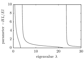
(a)

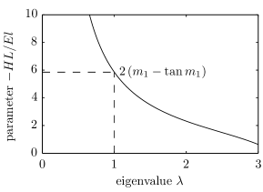
(b)

Figure 20: Relation between dimensionless parameter $-HL/El$ and eigenvalues of the first kind.

Let us first examine (80)–(82), having a nontrivial solution if and only if

$$2\omega^{-4}\sin\omega m_{1}\sinh\omega m_{1}-\left(\frac{m_{1}}{\omega^{3}}+\frac{HL\omega}{2El}\right)\left(\cos\omega m_{1}\sinh\omega m_{1}+\sin\omega m_{1}\cosh\omega m_{1}\right)=0$$ (85)

which is equivalent to

$$\frac{2}{\omega^{5}}\left(m_{1}\omega-\frac{2\sin\omega m_{1}\sinh\omega m_{1}}{\cos\omega m_{1}\sinh\omega m_{1}+\sin\omega m_{1}\cosh\omega m_{1}}\right)=-\frac{HL}{El}$$ (86)

Positive solutions of this transcendental equation, $\omega^{(1)}_{i}$, $i=1,2,\ldots$, correspond to eigenvalues $\lambda^{(1)}_{i}=\left(\omega^{(1)}_{i}\right)^{4}$, $i=1,2,\ldots$. Superscript ⁽¹⁾ means that we are dealing with solutions of the “first kind”, resulting from singularity of (80)–(82), with nonzero constants $C_{0}$, $C_{1}$ and $C_{3}$ and with $C_{2}=C_{4}=0$. Consequently, the corresponding eigenfunctions are even. The eigenvalues cannot be expressed analytically, but one can characterize them graphically, by plotting the left-hand side of (86) as a function of $\lambda\equiv\omega^{4}$, as shown in Fig. 20. The vertical axis corresponds to the dimensionless ratio $-HL/El$. For a given bar, this ratio is fixed and the intersections of the corresponding horizontal line with the graph provide the eigenvalues for the considered case.

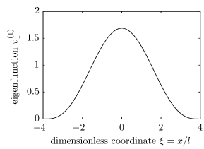
(a)

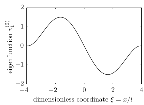
(b)

Figure 21: Eigenfunctions corresponding to the smallest eigenvalue (a) of the first kind, (b) of the second kind.

From Fig. 20 it is clear that if $-HL/El$ is at or above a certain critical value, the smallest eigenvalue of the first kind is smaller than or equal to 1 and the stability condition is violated. The critical value is obtained simply by evaluating the left-hand side of (86) for $\omega=1$, and turns out to be equal to $2\,(m_{1}-\tan m_{1})\doteq 5.8548$. Thus the resulting stability condition reads

$$-\frac{HL}{El}<2\,(m_{1}-\tan m_{1})$$ (87)

This is a constraint that involves the ratio between the absolute value of the softening modulus and the elastic modulus, $-H/E$, and the ratio between the bar length and the material characteristic length, $L/l$. Stability (under displacement control, i.e., with $\overline{u}$ prescribed) is compromised for long bars (large $L/l$) made of materials with pronounced softening (large $-H/E$). The eigenfunction

$$v^{(1)}_{1}=1-\frac{\cos\displaystyle\frac{x}{l}}{2\cos m_{1}}-\frac{\cosh\displaystyle\frac{x}{l}}{2\cosh m_{1}},\hskip 14.22636ptx\in\mathcal{I}_{p}\equiv(-m_{1}l,m_{1}l)$$ (88)

corresponding to the smallest eigenvalue of the first kind in the critical case when $\lambda^{(1)}_{1}=1$ (i.e., when $-{HL}/{El}=2\,(m_{1}-\tan m_{1})$) is plotted in Fig. 21a. Up to an arbitrary scalar multiplication factor, it is identical with the actual localized solution $\kappa(x)$ described in normalized form by equations (25) and (30). The critical case corresponds to a snapback point of the load-displacement diagram, i.e., to a point at which the tangent becomes vertical and the amplitude of the plastic strain profile can grow at constant total elongation of the bar while the equilibrium equation and the yield condition remain satisfied.

A.4 Odd Eigenfunctions

We still need to examine another set of eigenvalues, referred to as eigenvalues of the “second kind”. Equations (83)–(84) have a nontrivial solution if and only if

$$\sin\omega m_{1}\cosh\omega m_{1}-\cos\omega m_{1}\sinh\omega m_{1}=0$$ (89)

which is satisfied for

$$\omega^{(2)}_{i}=\frac{m_{i}}{m_{1}},\hskip 14.22636pti=1,2,\ldots$$ (90)

The corresponding eigenvalues and eigenfunctions of problem (76) are

$$\lambda^{(2)}_{i} =\left(\omega^{(2)}_{i}\right)^{4}=\left(\frac{m_{i}}{m_{1}}\right)^{4},\hskip 14.22636pti=1,2,\ldots$$ (91)

$$v^{(2)}_{i} =\frac{\sin\displaystyle\frac{m_{i}x}{m_{1}l}}{\sin m_{i}}-\frac{\sinh\displaystyle\frac{m_{i}x}{m_{1}l}}{\sinh m_{i}},\hskip 14.22636ptx\in\mathcal{I}_{p}\equiv(-m_{1}l,m_{1}l)$$ (92)

The smallest eigenvalue of the second kind, $\lambda^{(2)}_{1}$, is equal to 1, while all the others are greater than 1. All eigenfunctions of the second kind are odd, and the eigenfunction $v^{(2)}_{1}$ corresponding to the smallest eigenvalue is plotted in Fig. 21b.

A.5 Note on Larger Plastic Zones

The analysis presented so far for a uniform bar has referred exclusively to the localized solutions with the smallest possible plastic zone of size $L_{p}=2m_{1}l$. The original set of conditions (14)–(16), from which the plastic strain distribution $\kappa(x)$ was determined, may admit other solutions, with larger plastic zones. Indeed, the plastic zone size follows from equation (29), which has positive solutions $\lambda_{p}=m_{i}$, $i=1,2,\ldots$, corresponding to plastic zone sizes $L_{p}=2m_{i}l$, $i=1,2,\ldots$. In Section 3.1 we decided to focus on the most localized solution with $i=1$. If a uniform bar is long enough, there exist other solutions, corresponding to $i\geq 2$. An example for $i=2$ is plotted in Fig. 22a. Such solutions satisfy conditions that follow from non-negativeness of the first variation, but they violate the stability condition and thus cannot physically occur. To see that, consider the case of $i=2$, i.e., $\mathcal{I}_{p}=(-m_{2}l,m_{2}l)$ where $m_{2}\doteq 7.0686$. Condition (89) is then replaced by

$$\sin\omega m_{2}\cosh\omega m_{2}-\cos\omega m_{2}\sinh\omega m_{2}=0$$ (93)

Eigenvalues of the second kind are given by

$$\lambda^{(2)}_{i}=\left(\omega^{(2)}_{i}\right)^{4}=\left(\frac{m_{i}}{m_{2}}\right)^{4},\hskip 14.22636pti=1,2,\ldots$$ (94)

and the minimum eigenvalue, $\lambda^{(2)}_{1}=(m_{1}/m_{2})^{4}$, is smaller than 1. This indicates that condition (72) is violated and stability is lost. Fig. 22b shows the eigenfunction $v^{(2)}_{1}$ corresponding to the minimum eigenvalue.

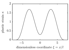
(a)

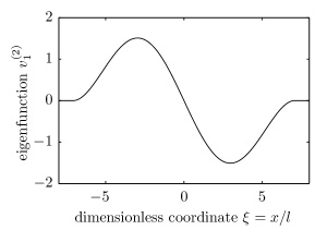
(b)

Figure 22: Eigenfunctions corresponding to the smallest eigenvalue (a) of the first kind, (b) of the second kind.

A.6 Summary

In summary, for a uniform bar (or sufficiently long uniform weakest segment of a bar) we have found that eigenvalues of the first kind are greater than 1 if the material constants and bar length satisfy a certain constraint, but the smallest eigenvalue of the second kind is always equal to 1. Strictly speaking, this would mean that stability cannot be guaranteed, because inequality (66) cannot be satisfied with any positive $\alpha$ but only with $\alpha=0$. The second variation is then non-negative but not positive definite. This is related to the special nature of the localization problem for a uniform bar, which actually admits infinitely many localized solutions characterized by the same energy level. Indeed, the precise position of the localized zone in a perfectly uniform bar remains undetermined, and the considered solution (centered in the middle of the bar) can be arbitrarily shifted without modifying the total energy. In a real bar, the position of the localized plastic zone would be affected by imperfections of the geometry and material data (sectional area, initial yield stress, etc.) For an ideal, perfectly uniform bar, the localized plastic zone can form anywhere and the corresponding solutions are neutrally stable. It is not by chance that the eigenfunction $v^{(2)}_{1}$ corresponding to eigenvalue $\lambda^{(2)}_{1}=1$ is actually a scalar multiple of the spatial derivative of function $\kappa$ which describes the plastic strain distribution. Adding an infinitely small multiple of $\kappa^{\prime}$ to $\kappa$ corresponds to an infinitesimal horizontal shift of the localized plastic strain profile. Note that adding a finite multiple of $\kappa^{\prime}$ would result into violation of the constraint $\kappa\geq 0$ near one boundary of the plastic zone and is thus inadmissible. Shifted plastic strain profiles form a parametric family of functions at the same energy level which does not correspond to a linear manifold in the functional space. Convex linear combinations of two selected members of this family correspond to higher energy levels and if the difference of two such functions is considered as a variation $\delta\kappa$, the corresponding first variation $\delta\Pi^{*}$ is positive. This is in agreement with our conclusion that variations which do not vanish everywhere in the elastic zone lead to positive $\delta\Pi^{*}$ and thus do not need to be considered in the stability analysis based on the second variation.

Before closing A, let us demonstrate the presented approach for a bar with a variable cross-sectional area. In particular, we verify $\lambda_{1}^{(2)}>1$ by numerically solving the eigenvalue problem (74) for a family of cross-sectional areas

$$\begin{aligned} A_{l}(x)&=1+\frac{a|x|}{1-a|x|}\\ A_{q}(x)&=1+\frac{(ax)^{2}}{1-(ax)^{2}}\end{aligned}\quad\quad\mbox{for }x\in\mathcal{I}_{p}\equiv(-m_{1}l,m_{1}l)$$ (95)

where $a\in[0,\frac{1}{m_{1}l})$, cf. also Eqs. (46) and (53), corresponding to piecewise linear and quadratic stress distributions. The obtained results are depicted in Fig. 23 where we verify that for $a\rightarrow 0$ we get $\lambda_{1}^{(2)}\rightarrow 1$, and that $\lambda_{1}^{(2)}>1$ for $a\neq 0$, as expected.

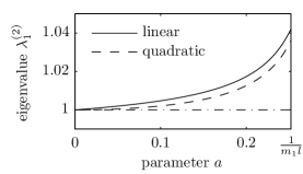
Figure 23: Eigenvalue of the second kind, $\lambda_{1}^{(2)}$, as a function of $a\in[0,\frac{1}{m_{1}l})$ for cross-sectional areas corresponding to piecewise linear and quadratic stress distributions, see Eq. (95).

This numerical result confirms that nonuniformity of the cross-section area $A(x)$ has a stabilizing effect.

Appendix B Stability of the Homogenenous Boundary Condition $\kappa^{\prime\prime}=0$

In order to verify that $\llbracket HAl^{4}\kappa^{\prime\prime}\rrbracket=0$ is the correct optimality condition at the elasto-plastic interface, we construct a family of solutions without taking this condition into account, and then prove that the energy-minizing state coincides with the solutions presented above.

For simplicity, we consider a uniform bar described by (25) with a symmetric general solution presented in (26), where $C_{2}=0$ and $C_{4}=0$, and where the boundary conditions read

$$\kappa_{n}(\lambda_{p})=0,\quad\kappa_{n}^{\prime}(\lambda_{p})=0$$ (96)

We have two conditions, but three unknowns, $C_{1}$, $C_{3}$ and $\lambda_{p}$. The last condition in (27), i.e. $\kappa^{\prime\prime}(\lambda_{p})=0$, is not imposed, but will be justified by direct energy minimization. Substituting (26) into (96) for $\lambda_{p}>0$ yields the solution

$$\kappa_{n}(\xi)=1-\phi-\frac{1-\phi}{\cos\lambda_{p}\sinh\lambda_{p}+\cosh\lambda_{p}\sin\lambda_{p}}(\sinh\lambda_{p}\cos\xi+\sin\lambda_{p}\cosh\xi)$$ (97)

In order to make our exposition more readable, the subsequent derivations are structured into four steps. In B.1, we first normalize the functional $\Pi^{*}$ from Eq. (61) in order to reparametrize it in terms of the dimensionless solution (97). Such a formulation makes it relatively easy to demonstrate that the homogeneous interface conditions correspond to a saddle point of the reduced energy functional, both under fixed axial force or prescribed displacements described in B.2 and B.3. In B.4 we finally demonstrate that the saddle points are energy minima.

B.1 Normalization of the Reduced Functional

We search for the minimizers of the energy functional $\Pi^{*}$, which after normalization takes the form

$$\overset{\circ}{\Pi}(\kappa_{n})=\psi\left(\widetilde{u}-\theta\int_{-\lambda_{p}}^{\lambda_{p}}\kappa_{n}\,\mathrm{d}\xi\right)^{2}+\psi\theta\int_{-\lambda_{p}}^{\lambda_{p}}(-\kappa_{n}^{2}+\kappa_{n}^{\prime\prime 2}+2\kappa_{n})\,\mathrm{d}\xi$$ (98)

where we have denoted

$$\theta=-\frac{El}{H2l_{g}}$$ (99)

In (98), $\widetilde{u}=\overline{u}/u_{0}$ denotes the dimensionless elongation, $u_{0}=2l_{g}\sigma_{r}/E=2l_{g}\varepsilon_{0}$, and $\psi=Al_{g}\sigma_{r}^{2}/E$ denotes the reference energy. Since $F=A\sigma_{r}\phi$, we rewrite (58) as

$$u^{\prime}-\kappa=\frac{F}{EA}=\frac{\sigma_{r}\phi}{E}$$ (100)

Integration over the plastic zone $\mathcal{I}_{p}$ and conversion to the normalized form provides

$$\phi=\widetilde{u}-\theta\int_{-\lambda_{p}}^{\lambda_{p}}\kappa_{n}\,\mathrm{d}\xi$$ (101)

see also (59), which can be introduced into the energy functional (98) and furnishes us with the relation

$$\overset{\circ}{\Pi}(\kappa_{n})=\psi\phi^{2}+\psi\theta\int_{-\lambda_{p}}^{\lambda_{p}}(-\kappa_{n}^{2}+\kappa_{n}^{\prime\prime 2}+2\kappa_{n})\,\mathrm{d}\xi$$ (102)

Two situations can now be investigated: minimization under fixed axial force $\phi$, or under prescribed displacement $\widetilde{u}$. Note that, for a prismatic bar with uniform properties in inelastic regime, we have $\phi<1$, which can be verified in Figs. 4b and 12b for $\beta\rightarrow 0$ or Eq. (31), and that $\widetilde{u}>1$ directly from its definition.

B.2 The case of fixed $\phi$

Direct differentiation and integration of (97) provides

$$\int_{-\lambda_{p}}^{\lambda_{p}}\kappa_{n}\,\mathrm{d}\xi=2(1-\phi)(\lambda_{p}-2\alpha)$$ (103a)

$$\int_{-\lambda_{p}}^{\lambda_{p}}(-\kappa_{n}^{2}+\kappa_{n}^{\prime\prime 2})\,\mathrm{d}\xi=2(1-\phi^{2})(\lambda_{p}-2\alpha)$$ (103b)

where we have denoted

$$\alpha(\lambda_{p})=\frac{\sinh\lambda_{p}\sin\lambda_{p}}{\cos\lambda_{p}\sinh\lambda_{p}+\cosh\lambda_{p}\sin\lambda_{p}}$$ (104)

Substituting from (103) into (102) gives after some algebra

$$\widehat{\Pi}(\lambda_{p})=\psi\left\{\phi^{2}+2\theta(1-\phi^{2})[\lambda_{p}-2\alpha(\lambda_{p})]\right\}$$ (105)

from which we obtain the stationarity condition (the prime now denotes the derivative with respect to $\lambda_{p}$)

$$\widehat{\Pi}^{\prime}(\lambda_{p})=2\theta\psi(1-\phi^{2})\frac{\mathrm{d}}{\mathrm{d}\lambda_{p}}[\lambda_{p}-2\alpha(\lambda_{p})]=0$$ (106)

which reduces to (29) and hence $\lambda_{p}=m_{1}$. Taking the second derivative provides

$$\left.\frac{\mathrm{d}^{2}}{\mathrm{d}\lambda_{p}^{2}}[\lambda_{p}-2\alpha(\lambda_{p})]\right|_{\lambda_{p}=m_{1}}=-2\left.\frac{\mathrm{d}^{2}}{\mathrm{d}\lambda_{p}^{2}}\alpha(\lambda_{p})\right|_{\lambda_{p}=m_{1}}=0$$ (107)

From Fig. 24 and Eq. (107) we deduce that $\lambda_{p}=m_{1}$ is a saddle point of $\widehat{\Pi}$.

B.3 The case of fixed $\widetilde{u}$

Introducing (103a) into Eq. (101) provides

$$\phi(\lambda_{p})=\frac{\widetilde{u}-2\theta[\lambda_{p}-2\alpha(\lambda_{p})]}{1-2\theta[\lambda_{p}-2\alpha(\lambda_{p})]}=1-\frac{\widetilde{u}-1}{D(\lambda_{p})}$$ (108)

where we have denoted $D(\lambda_{p})=1-2\theta[\lambda_{p}-2\alpha(\lambda_{p})]$. Substituting (108) into (105) then gives

$$\widetilde{\Pi}(\lambda_{p})=\psi\left\{\frac{[1-D(\lambda_{p})](1-2\widetilde{u})+\widetilde{u}^{2}}{D(\lambda_{p})}\right\}$$ (109)

which is the normalized energy functional under prescribed fixed dimensionless elongation $\widetilde{u}$. Minimization with respect to $\lambda_{p}$ yields

$$\widetilde{\Pi}^{\prime}(\lambda_{p})=-\frac{\psi(1-\widetilde{u})^{2}}{D^{2}(\lambda_{p})}\frac{\mathrm{d}}{\mathrm{d}\lambda_{p}}D(\lambda_{p})=2\psi\theta\frac{(1-\widetilde{u})^{2}}{D^{2}(\lambda_{p})}\frac{\mathrm{d}}{\mathrm{d}\lambda_{p}}[\lambda_{p}-2\alpha(\lambda_{p})]=0$$ (110)

The condition $\frac{\mathrm{d}}{\mathrm{d}\lambda_{p}}[\lambda_{p}-\alpha(\lambda_{p})]=0$ reduces again to Eq. (29), cf also (106). The second derivative of $\widetilde{\Pi}$ provides again condition (107) showing that the solution is also at a saddle point.

B.4 Energy minima

To verify that $\lambda_{p}=m_{1}$ is actually the minimum, we recall the geometric constraint $\kappa_{n}^{\prime\prime}(\lambda_{p})\geq 0$ resulting from the requirements that $\kappa(\lambda_{p})=0,\kappa^{\prime}(\lambda_{p})=0$, $\kappa(\xi)\geq 0$, $\kappa(\xi)=0$ for $\xi\notin(-\lambda_{p},\lambda_{p})$, and a Taylor series expansion in $\mathcal{I}_{p}$ near the boundary point $\lambda_{p}$. Consequently, the constraint $\kappa_{n}^{\prime\prime}(\lambda_{p})\geq 0$ gives for the general solution in (97) condition $\sinh\lambda_{p}\cos\lambda_{p}-\sin\lambda_{p}\cosh\lambda_{p}\geq 0$, which provides the constraint $\lambda_{p}\in[n_{1},m_{1}]$. For the definition of $m_{1}$ see Eq. (29) and the discussion below; analogously we define $n_{i}$ as solutions of $\tan n_{i}=-\tanh n_{i}$, which leads to $n_{\pm i}\doteq 0,\pm 2.3650,\pm 5.4978,\dots,i\in\mathbb{N}_{0}$. Since

$$\widehat{\Pi}^{\prime}(\lambda_{p})=\widetilde{\Pi}^{\prime}(\lambda_{p}) =C_{\Pi}\frac{\mathrm{d}}{\mathrm{d}\lambda_{p}}[\lambda_{p}-2\alpha(\lambda_{p})]$$ (111)

$$=-C_{\Pi}\frac{(\cosh\lambda_{p}\sin\lambda_{p}-\cos\lambda_{p}\sinh\lambda_{p})^{2}}{(\cosh\lambda_{p}\sin\lambda_{p}+\cos\lambda_{p}\sinh\lambda_{p})^{2}}\ \left\{\begin{aligned} &<0\mbox{ for }\lambda_{p}\in[n_{1},m_{1})\\ &=0\mbox{ for }m_{1}\end{aligned}\right.$$

where $C_{\Pi}>0$ is a $\lambda_{p}$-independent constant, cf. Eqs. (106) and (110), we conclude that the minimum is attained for $\lambda_{p}=m_{1}$. This finding can be visually verified in Fig. 24 constructed for the data from Tab. 2, for $L=2l_{g}=4lm_{1}$, and for the load parameters $\phi=0.5$ or $\widetilde{u}=3$.

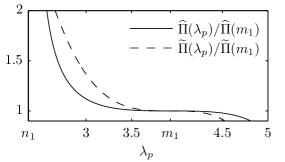
Figure 24: $\widehat{\Pi}(\lambda_{p})/\widehat{\Pi}(m_{1})$ for fixed $\phi=0.5$, and $\widetilde{\Pi}(\lambda_{p})/\widetilde{\Pi}(m_{1})$ for fixed $\widetilde{u}=3$ as functions of $\lambda_{p}\in[n_{1},m_{1}]$ and for a bar with uniform properties.

In conclusion, for both cases, i.e. either for fixed $\phi$ or $\widetilde{u}$, the boundary condition $\kappa_{n}^{\prime\prime}(\lambda_{p})=0$ is indeed the optimal one and the solution is located at a saddle point, which is at the same time the boundary of the admissible set $[n_{1},m_{1}]$.

References

- Alessi et al. (2014) Alessi, R., Marigo, J.-J., Vidoli, S., 2014. Gradient damage models coupled with plasticity and nucleation of cohesive cracks. Archive for Rational Mechanics and Analysis 214 (2), 575–615. doi:10.1007/s00205-014-0763-8.
- Almkvist et al. (2011) Almkvist, G., van Straten, D., Zudilin, W., 2011. Generalizations of Clausen’s formula and algebraic transformations of Calabi-Yau differential equations. Proceedings of the Edinburgh Mathematical Society. Series II 54 (2), 273–295. doi:10.1017/S0013091509000959.
- Bažant and Jirásek (2002) Bažant, Z. P., Jirásek, M., 2002. Nonlocal integral formulations of plasticity and damage: Survey of progress. Journal of Engineering Mechanics ASCE 128, 1119–1149. doi:10.1061/(ASCE)0733-9399(2002)128:11(1119).
- Braides (2014) Braides, A., 2014. Local Minimization, Variational Evolution and -Convergence. No. 2094 in Lecture Notes in Mathematics. Springer, New York.
- Carstensen et al. (2002) Carstensen, C., Hackl, K., Mielke, A., 2002. Non-convex potentials and microstructures in finite-strain plasticity. Proceedings of the Royal Society of London A: Mathematical, Physical and Engineering Sciences 458 (2018), 299–317. doi:10.1098/rspa.2001.0864.
- de Vree et al. (1995) de Vree, J. H. P., Brekelmans, W. A. M., van Gils, M. A. J., 1995. Comparison of nonlocal approaches in continuum damage mechanics. Computers and Structures 55, 581–588. doi:10.1016/0045-7949(94)00501-S.
- Del Piero et al. (2013) Del Piero, G., Lancioni, G., March, R., 2013. A diffuse cohesive energy approach to fracture and plasticity: the one-dimensional case. Journal of Mechanics of Materials and Structures 8 (2-4), 109–151. doi:10.2140/jomms.2013.8.109.
- Evans (2010) Evans, L. C., 2010. Partial Differential Equations, 2nd Edition. Vol. 19 of Graduate Studies in Mathematics. American Mathematical Society, Providence, Rhode Island.
- Francfort and Marigo (1993) Francfort, G. A., Marigo, J.-J., 1993. Stable damage evolution in a brittle continuous medium. European Journal of Mechanics. A. Solids 12 (2), 149–189.
- Francfort and Marigo (1998) Francfort, G. A., Marigo, J.-J., 1998. Revisiting brittle fracture as an energy minimization problem. Journal of the Mechanics and Physics of Solids 46 (8), 1319–1342. doi:10.1016/S0022-5096(98)00034-9.
- Iurlano (2013) Iurlano, F., 2013. Fracture and plastic models as -limits of damage models under different regimes. Advances in Calculus of Variations 6 (2), 165–189. doi:10.1515/acv-2011-0011.
- Jirásek (1998) Jirásek, M., 1998. Nonlocal models for damage and fracture: Comparison of approaches. International Journal of Solids and Structures 35, 4133–4145.
- Jirásek et al. (2013) Jirásek, M., Rokoš, O., Zeman, J., 2013. Localization analysis of variationally based gradient plasticity model. International Journal of Solids and Structures 50 (1), 256–269. doi:http://dx.doi.org/10.1016/j.ijsolstr.2012.09.022.
- Jirásek and Rolshoven (2003) Jirásek, M., Rolshoven, S., 2003. Comparison of integral-type nonlocal plasticity models for strain-softening materials. International Journal of Engineering Science 41, 1553–1602. doi:10.1016/S0020-7225(03)00027-2.
- Jirásek and Rolshoven (2009a) Jirásek, M., Rolshoven, S., 2009a. Localization properties of strain-softening gradient plasticity models. Part I: Strain-gradient theories. International Journal of Solids and Structures 46, 2225–2238. doi:10.1016/S0020-7225(03)00027-2.
- Jirásek and Rolshoven (2009b) Jirásek, M., Rolshoven, S., 2009b. Localization properties of strain-softening gradient plasticity models. Part II: Theories with gradients of internal variables. International Journal of Solids and Structures 46 (11–12), 2239–2254. doi:10.1016/j.ijsolstr.2008.12.018.
- Jirásek and Zeman (2015) Jirásek, M., Zeman, J., 2015. Localization study of a regularized variational damage model. International Journal of Solids and Structures 69–70, 131–151. doi:10.1016/j.ijsolstr.2015.06.001.
- Jirásek et al. (2010) Jirásek, M., Zeman, J., Vondřejc, J., 2010. Softening gradient plasticity: Analytical study of localization under nonuniform stress. International Journal for Multiscale Computational Engineering 8 (1), 37–60. doi:10.1615/IntJMultCompEng.v8.i1.40.
- Lellis and Royer-Carfagni (2001) Lellis, C. D., Royer-Carfagni, G., 2001. Interaction of fractures in tensile bars with non-local spatial dependence. Journal of Elasticity 65 (1–3), 1–31. doi:10.1023/A:1016143321232.
- Mielke (2003) Mielke, A., 2003. Energetic formulation of multiplicative elasto-plasticity using dissipation distances. Continuum Mechanics and Thermodynamics 15 (4), 351–382. doi:10.1007/s00161-003-0120-x.
- Mielke (2006) Mielke, A., 2006. Evolution of rate-independent systems. In: Dafermos, C. M., Feireisl, E. (Eds.), Handbook of Differential Equations: Evolutionary Equations. Vol. 2. North-Holland, Ch. 6, pp. 461–559.
- Mielke (2011) Mielke, A., 2011. Differential, energetic, and metric formulations for rate-independent processes. In: Ambrosio, L., Savaré, G. (Eds.), Nonlinear PDE’s and Applications. No. 2011 in Lecture Notes in Mathematics. Springer, Berlin, Heidelberg, pp. 87–170.
- Mielke and Theil (2004) Mielke, A., Theil, F., 2004. On rate-independent hysteresis models. Nonlinear Differential Equations and Applications NoDEA 11 (2), 151–189. doi:10.1007/s00030-003-1052-7.
- Milašinović (2004) Milašinović, D. D., 2004. Rheological–dynamical analogy: Visco-elasto-plastic behavior of metallic bars. International Journal of Solids and Structures 41 (16), 4599–4634. doi:10.1016/j.ijsolstr.2004.02.061.
- Mühlhaus and Aifantis (1991) Mühlhaus, H. B., Aifantis, E., 1991. A variational principle for gradient plasticity. International Journal of Solids and Structures 28 (7), 845–857. doi:http://dx.doi.org/10.1016/0020-7683(91)90004-Y.
- Ortiz and Stainier (1999) Ortiz, M., Stainier, L., 1999. The variational formulation of viscoplastic constitutive updates. Computer Methods in Applied Mechanics and Engineering 171 (3–4), 419–444. doi:10.1016/S0045-7825(98)00219-9.
- Peerlings et al. (2001) Peerlings, R. H. J., Geers, M. G. D., de Borst, R., Brekelmans, W. A. M., 2001. A critical comparison of nonlocal and gradient-enhanced softening continua. International Journal of Solids and Structures 38, 7723–7746. doi:10.1016/j.ijsolstr.2004.02.061.
- Petryk (2003) Petryk, H., 2003. Incremental energy minimization in dissipative solids. Comptes Rendus Mécanique 331 (7), 469–474. doi:10.1016/S1631-0721(03)00109-8.
- Pham and Marigo (2013) Pham, K., Marigo, J.-J., 2013. From the onset of damage to rupture: construction of responses with damage localization for a general class of gradient damage models. Continuum Mechanics and Thermodynamics 25 (2–4), 147–171. doi:10.1007/s00161-011-0228-3.
- Pham et al. (2011) Pham, K., Marigo, J.-J., Maurini, C., 2011. The issues of the uniqueness and the stability of the homogeneous response in uniaxial tests with gradient damage models. Journal of the Mechanics and Physics of Solids 59 (6), 1163–1190. doi:10.1016/j.jmps.2011.03.010.
- Roubíček (2010) Roubíček, T., 2010. Nonlinear Partial Differential Equations with Applications, 2nd Edition. Vol. 153 of International Series of Numerical Mathematics. Birkhaüser-Verlag, Basel, Boston, Berlin. doi:10.1007/978-3-0348-0513-1.
- Roubíček (2015) Roubíček, T., 2015. Maximally-dissipative local solutions to rate-independent systems and application to damage and delamination problems. Nonlinear Analysis: Theory, Methods & Applications 113, 33–50. doi:10.1016/j.na.2014.09.020.
- Šebestová and Vejchodský (2014) Šebestová, I., Vejchodský, T., 2014. Two-sided bounds for eigenvalues of differential operators with applications to Friedrichs, Poincaré, trace, and similar constants. SIAM Journal on Numerical Analysis 52 (1), 308–329. doi:10.1137/13091467X.
- Shampine et al. (2003) Shampine, L. F., Gladwell, I., Thompson, S., 2003. Solving ODEs with MATLAB. Cambridge University Press, Cambridge.
- Zbib and Aifantis (1988) Zbib, H. M., Aifantis, E. C., 1988. On the localization and postlocalization behavior of plastic deformation. Res Mechanica 23, 261–305.