Numerical Simulations of Bouncing Jets

Andrea Bonito111Partially supported by the NSF grant DMS-1254618 and by award KUS-C1-016-04 made by King Abdullah University of Science and Technology (KAUST) bonito@math.tamu.edu Jean-Luc Guermond guermond@math.tamu.edu Sanghyun Lee222Partially supported by the NSF grant DMS-1254618 and by award KUS-C1-016-04 made by King Abdullah University of Science and Technology (KAUST) shlee@math.tamu.edu Department of Mathematics, Texas A&M University,
College Station, Texas 77843-3368, USA
Abstract

Bouncing jets are fascinating phenomenons occurring under certain conditions when a jet impinges on a free surface. This effect is observed when the fluid is Newtonian and the jet falls in a bath undergoing a solid motion. It occurs also for non-Newtonian fluids when the jets falls in a vessel at rest containing the same fluid. We investigate numerically the impact of the experimental setting and the rheological properties of the fluid on the onset of the bouncing phenomenon. Our investigations show that the occurrence of a thin lubricating layer of air separating the jet and the rest of the liquid is a key factor for the bouncing of the jet to happen. The numerical technique that is used consists of a projection method for the Navier-Stokes system coupled with a level set formulation for the representation of the interface. The space approximation is done with adaptive finite elements. Adaptive refinement is shown to be very important to capture the thin layer of air that is responsible for the bouncing.

keywords:
Bouncing Jet , Kaye effect , Entropy Viscosity , Level set , Projection Method , Shear-thinning viscosity , Adaptive Finite Elements
journal: Journal of Computational Physics

1 Introduction

The ability of a jet of fluid to bounce on a free surface has been observed in different contexts. Thrasher et al. [31] designed an experiment where a jet of Newtonian fluid falls into a rotating vessel filled with the same fluid. The authors investigated the conditions under which the jet bounces: nature of the fluid, jet diameter, jet and bath velocities. We refer to Lockhart [26] for experimental movies illustrating this effect.
Refer to caption
Refer to caption
Refer to caption
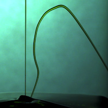
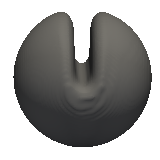
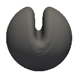
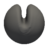
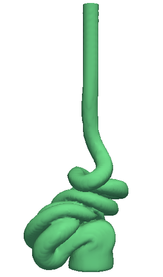
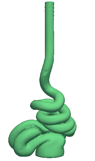
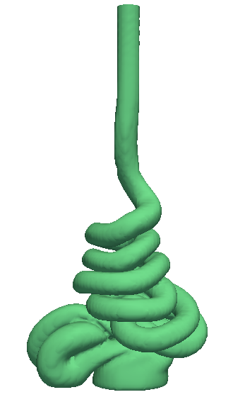
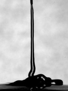
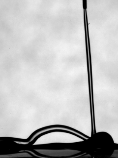
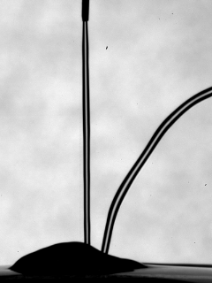
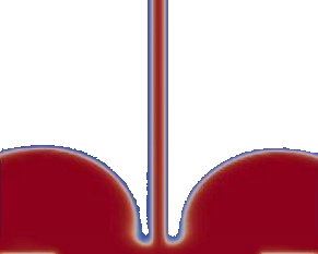
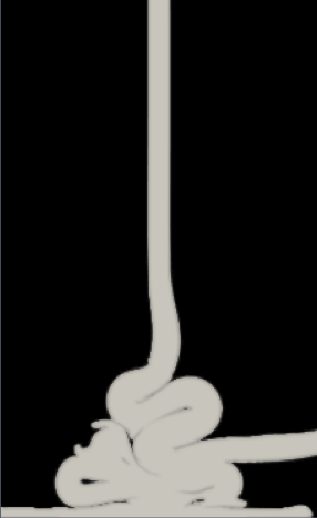
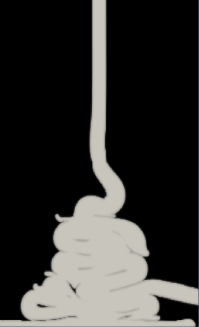
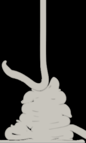
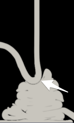
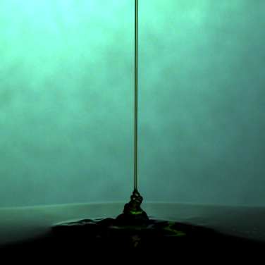
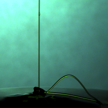
Figure 1: Experimental Observation of the Kaye Effect. (Left) the fluid start to buckle producing a heap; (middle) A stream of liquid suddenly leaps outside the heap; (right) Fully developed Kaye effect.

Bouncing can also be observed in a stationary vessel provided the jet is composed of a non-newtonian fluid. During the pouring process, a small heap of fluid forms and the jet occasionally leaps upward from the heap; see Figure 1. This is the so-called Kaye effect as first observed by Kaye [24] in 1963. About 13 years after this phenomenon was first mentioned in the literature, Collyer and Fischer [12] revisited the experiment and suggested that the ability for the fluid to exhibit shear-thinning viscosity and elastic behavior are key ingredients for the bouncing to occur. Additional laboratory experiments performed by Versluis et al. [34] and Binder and Landig [5] lead the authors of each team to propose a list of properties that the fluid should have for the Kaye effect to occur. The conclusions of these two papers disagree on the requirement that the fluid be elastic and on the nature of the thin layer that separates the heap and the outgoing jet. It is argued in Versluis et al. [34] that elastic properties are not necessary and that the thin layer is a shear layer, whereas it is argued in Binder and Landig [5] that the fluid should have elastic properties and that the thin layer separating the heap from the bouncing jet is a layer of air. Recent experiments reported in Lee et al. [25] using a high speed camera unambiguously show that the jet slides on a lubricating layer of air. For completeness, we also refer to Ochoa et al. [27] for a thorough discussion on the “stable” Kaye effect, where the jet falls against an inclined surface.

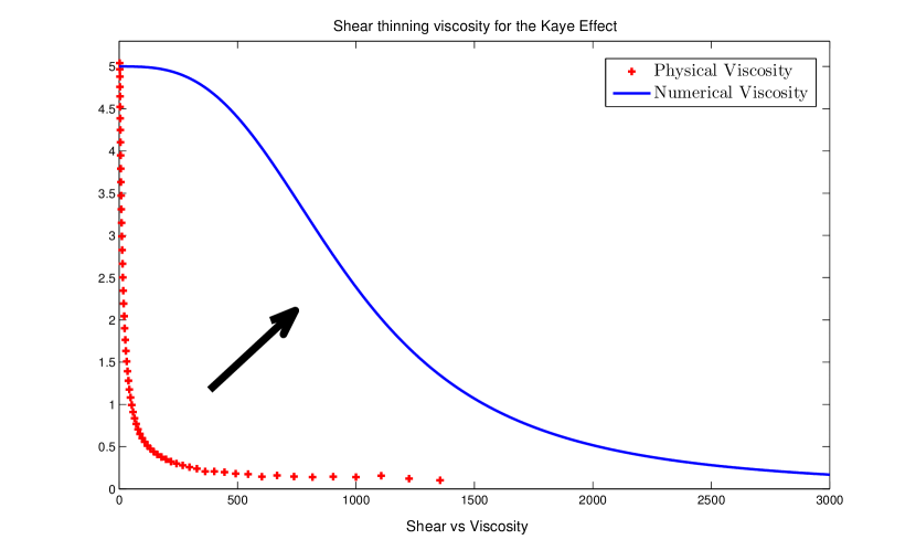
The objective of the present paper is to numerically revisit the Kaye effect. Our key finding is that a thin air layer is always present between the bouncing jet and the rest of the fluid whether the fluid is Newtonian or not. Our numerical experiments suggest that the critical parameter for bouncing to occur is that the properties of fluid and the experimental conditions be such that a stable layer of air separating the jet and the ambiant fluid can appear. This condition is met by setting the bath in motion for Newtonian fluids; it can also be met if the bath is stationary provided the fluid is non-Newtonian and has shear-thinning viscosity. The numerical code that we use is based on a modeling the fluid flows by the incompressible Navier-Stokes equations supplemented with a surface tension mechanism. The shear-thinning viscosity of the non-Newtonian fluids is assumed to follow a model by Cross [13]. Elastic behaviors are not modeled. The numerical approximation of the resulting two-phase flow model is based on two solvers: one solving the Navier-Stokes equations assuming that the fluid/air distribution is given, the other keeping track of the motion of the interface assuming the transport velocity is given. The Navier-Stokes solver is based on projection method by Chorin [11] and Témam [30] using a second-order backward differentiation formula for the time discretization and finite elements for the space approximation. The transport solver is based on a level-set technique in the spirit of Osher and Sethian [28] to represent the liquid/air interface. The level set is approximated in space by using finite elements and the time stepping is done by using a third order explicit Runge-Kutta technique.

The paper is organized as follows. The mathematical model is presented in Section 2. The numerical techniques to solve the Navier-Stokes equations and the transport equation for the level set function are described in Section 3. Various validation tests of the numerical algorithms and comparisons with classical benchmark problems are reported in Section 4. Finally, we report numerical evidences of Newtonian and non-Newtonian bouncing jets in Section 5.

2 The Mathematical Model

This section presents the mathematical models adopted to describe non-mixing two phase fluid flows with capillary forces. Each fluid is assumed to be incompressible.

2.1 Two Phase Flow System

Let ΛdΛsuperscript𝑑\Lambda\subset\mathbb{R}^{d} (d=2,3𝑑23d=2,3) be an open and bounded computational domain with Lipschitz boundary ΛΛ\partial\Lambda and let [0,T]0𝑇[0,T] be the computational time interval, T>0𝑇0T>0. The cavity ΛΛ\Lambda is filled with two non-mixing fluids undergoing some time-dependent motion, say fluid 1 and fluid 2. We denote by Ω+superscriptΩ\Omega^{+} and ΩsuperscriptΩ\Omega^{-} the open subsets of the space-time domain Λ×[0,T]Λ0𝑇\Lambda{\times}[0,T] occupied by fluid 1 and fluid 2, respectively. We denote by ρ+superscript𝜌\rho^{+}, μ+superscript𝜇\mu^{+}, ρsuperscript𝜌\rho^{-}, μsuperscript𝜇\mu^{-} the density and dynamical viscosity of each fluid, respectively. The interface between the two fluids in the space-time domain is denoted Σ:=Ω+ΩassignΣsuperscriptΩsuperscriptΩ\Sigma:=\partial\Omega^{+}\cap\partial\Omega^{-}, and the normal to ΣΣ\Sigma, oriented from Ω+superscriptΩ\Omega^{+} to ΩsuperscriptΩ\Omega^{-}, is denoted 𝐧Σsubscript𝐧Σ{\bf n}_{\Sigma}. The two space-time components of the vector field 𝐧Σ:Σd×:subscript𝐧ΣΣsuperscript𝑑{\bf n}_{\Sigma}:\Sigma\longrightarrow\mathbb{R}^{d}{\times}\mathbb{R} are denoted 𝐧𝐧{\bf n} and 𝐧τsubscript𝐧𝜏{\bf n}_{\tau}, respectively. It is also useful to define Ω±(t):=Ω±(Λ×{t})assignsuperscriptΩplus-or-minus𝑡superscriptΩplus-or-minusΛ𝑡\Omega^{\pm}(t):=\Omega^{\pm}\cap(\Lambda{\times}\{t\}); i.e., the sets Ω+(t)superscriptΩ𝑡\Omega^{+}(t) and Ω(t)superscriptΩ𝑡\Omega^{-}(t) are the regions occupied by fluid 1 and fluid 2 at time t𝑡t, respectively. We also introduce the interface Σ(t)=Ω+(t)Ω(t)Σ𝑡superscriptΩ𝑡superscriptΩ𝑡\Sigma(t)=\partial\Omega^{+}(t)\cap\partial\Omega^{-}(t); note that 𝐧𝐧{\bf n}, as defined above, is the unit normal of Σ(t)Σ𝑡\Sigma(t) and it is oriented from Ω+(t)superscriptΩ𝑡\Omega^{+}(t) to Ω(t)superscriptΩ𝑡\Omega^{-}(t). To facilitate the modeling, we define global density and dynamical viscosity functions ρ,μ:Λ×[0,T]:𝜌𝜇Λ0𝑇\rho,\mu:\Lambda{\times}[0,T]\rightarrow\mathbb{R} by setting ρ(𝐱,t)=ρ±𝜌𝐱𝑡superscript𝜌plus-or-minus\rho({\bf x},t)=\rho^{\pm} and μ(𝐱,t)=μ±𝜇𝐱𝑡superscript𝜇plus-or-minus\mu({\bf x},t)=\mu^{\pm} if (𝐱,t)Ω±𝐱𝑡superscriptΩplus-or-minus({\bf x},t)\in\Omega^{\pm}. The fluid velocity field 𝐮:Λ×[0,T]d:𝐮Λ0𝑇superscript𝑑{{\bf u}}:\Lambda{\times}[0,T]\rightarrow\mathbb{R}^{d}, henceforth assumed to be continuous across ΣΣ\Sigma, and the pressure p:Λ×[0,T]:𝑝Λ0𝑇p:\Lambda{\times}[0,T]\rightarrow\mathbb{R} are defined globally and solve the incompressible Navier-Stokes equations in the distribution sense in the space-time domain

ρ(t𝐮+𝐮𝐮)2div(μS𝐮)+pδΣσκ𝐧𝜌𝑡𝐮𝐮𝐮2div𝜇superscript𝑆𝐮𝑝subscript𝛿Σ𝜎𝜅𝐧\displaystyle\rho\left(\dfrac{\partial}{\partial t}{\bf u}+{\bf u}{\cdot}\nabla{\bf u}\right)-2\mbox{div}\left(\mu\ \nabla^{S}{\bf u}\right)+\nabla p-\delta_{\Sigma}\sigma\kappa{\bf n} =ρ𝐠absent𝜌𝐠\displaystyle=\rho{\bf g} in Λ×(0,T],Λ0𝑇\displaystyle\Lambda{\times}(0,T], (1a)
div(𝐮)div𝐮\displaystyle\mathrm{div}({\bf u}) =0absent0\displaystyle=0 in Λ×(0,T],Λ0𝑇\displaystyle\Lambda{\times}(0,T], (1b)

where S𝐮:=12(𝐮+𝐮T)assignsuperscript𝑆𝐮12𝐮superscript𝐮𝑇\nabla^{S}{\bf u}:=\frac{1}{2}(\nabla{\bf u}+\nabla{\bf u}^{T}) is the strain rate tensor, 𝐠𝐠{\bf g} is the gravity field, and δΣσκ𝐧subscript𝛿Σ𝜎𝜅𝐧\delta_{\Sigma}\sigma\kappa{\bf n} is a singular measure modeling the surface tension acting on Σ(t)Σ𝑡\Sigma(t). The distribution δΣsubscript𝛿Σ\delta_{\Sigma} is the Dirac measure supported on ΣΣ\Sigma, the function κ:Σ:𝜅Σ\kappa:\Sigma\rightarrow\mathbb{R} is the total curvature of Σ(t)Σ𝑡\Sigma(t) (sum of the principal curvatures) and σ𝜎\sigma is the surface tension coefficient.

The system (1) is supplemented with initial and boundary conditions. The initial condition is 𝐮(𝐱,0)=𝐮0(𝐱)𝐮𝐱0subscript𝐮0𝐱{\bf u}({\bf x},0)={\bf u}_{0}({\bf x}) for all 𝐱Λ𝐱Λ{\bf x}\in\Lambda, where 𝐮0subscript𝐮0{\bf u}_{0} is assumed to be a smooth divergence-free velocity field. The boundary ΛΛ\partial\Lambda is decomposed into three non-overlapping components Λ:=Γ¯DΓ¯NΓ¯NassignΛsubscript¯Γ𝐷subscript¯Γ𝑁subscript¯Γ𝑁\partial\Lambda:=\overline{\Gamma}_{D}\cup\overline{\Gamma}_{N}\cup\overline{\Gamma}_{N} with ΓDΓN=subscriptΓ𝐷subscriptΓ𝑁\Gamma_{D}\cap\Gamma_{N}=\emptyset, ΓNΓS=subscriptΓ𝑁subscriptΓ𝑆\Gamma_{N}\cap\Gamma_{S}=\emptyset, ΓSΓD=subscriptΓ𝑆subscriptΓ𝐷\Gamma_{S}\cap\Gamma_{D}=\emptyset. Time-dependent decomposition could be considered but are not described here to avoid unnecessary technicalities. Given 𝐟N:ΓNd:subscript𝐟𝑁subscriptΓ𝑁superscript𝑑{\bf f}_{N}:\Gamma_{N}\rightarrow\mathbb{R}^{d} and 𝐟D:ΓDd:subscript𝐟𝐷subscriptΓ𝐷superscript𝑑{\bf f}_{D}:\Gamma_{D}\rightarrow\mathbb{R}^{d}, we require that

(2μS𝐮pI)𝝂2𝜇superscript𝑆𝐮𝑝𝐼𝝂\displaystyle\left(2\mu\nabla^{S}{\bf u}-pI\right){\boldsymbol{\nu}} =𝐟N,absentsubscript𝐟𝑁\displaystyle={\bf f}_{N}, on ΓN×(0,T],subscriptΓ𝑁0𝑇\displaystyle\Gamma_{N}{\times}(0,T], (2a)
𝐮𝐮\displaystyle{\bf u} =𝐟D,absentsubscript𝐟𝐷\displaystyle={\bf f}_{D}, on ΓD×(0,T],subscriptΓ𝐷0𝑇\displaystyle\Gamma_{D}{\times}(0,T], (2b)
𝐮𝝂=0,((2μS𝐮pI)𝝂)×𝝂𝐮𝝂02𝜇superscript𝑆𝐮𝑝𝐼𝝂𝝂\displaystyle{\bf u}{\cdot}{\boldsymbol{\nu}}=0,\quad\left(\left(2\mu\nabla^{S}{\bf u}-pI\right){\boldsymbol{\nu}}\right){\times}{\boldsymbol{\nu}} =0,absent0\displaystyle=0, on ΓS×(0,T],subscriptΓ𝑆0𝑇\displaystyle\Gamma_{S}{\times}(0,T], (2c)

where 𝝂𝝂{\boldsymbol{\nu}} is the outward pointing unit normal on ΛΛ\partial\Lambda and I𝐼I is the d×d𝑑𝑑d{\times}d identity matrix. For simplicity, we assume that the (d1)𝑑1(d-1)-measures of ΓNΓSsubscriptΓ𝑁subscriptΓ𝑆\Gamma_{N}\cup\Gamma_{S} and ΓDsubscriptΓ𝐷\Gamma_{D} are each strictly positive; otherwise extra constraints either on the velocity or on the pressure must be enforced.

Note that we could have formulated the conservation of momentum without invoking the singular measure modeling the surface tension by saying that (1a) holds in Ω+superscriptΩ\Omega^{+} and ΩsuperscriptΩ\Omega^{-} (without the singular measure) and by additionally requiring that

[𝐮]=0and[2μS𝐮pI]𝐧=σκ𝐧onΣ(t),t(0,T],formulae-sequencedelimited-[]𝐮0andformulae-sequencedelimited-[]2𝜇superscript𝑆𝐮𝑝𝐼𝐧𝜎𝜅𝐧onΣ𝑡for-all𝑡0𝑇[{\bf u}]=0\quad\text{and}\quad\left[2\mu\nabla^{S}{\bf u}-pI\right]{\bf n}=\sigma\kappa{\bf n}\quad\text{on}\quad\Sigma(t),\qquad\forall t\in(0,T], (3)

where [.][.] denotes the jump across Σ(t)Σ𝑡\Sigma(t) defined by [𝐯](𝐱):=limΩ𝐲𝐱𝐯(𝐲)limΩ+𝐳𝐱𝐯(𝐳)assigndelimited-[]𝐯𝐱subscriptcontainssuperscriptΩ𝐲𝐱𝐯𝐲subscriptcontainssuperscriptΩ𝐳𝐱𝐯𝐳[{\bf v}]({\bf x}):=\lim_{\Omega^{-}\ni{\bf y}\to{\bf x}}{\bf v}({\bf y})-\lim_{\Omega^{+}\ni{\bf z}\to{\bf x}}{\bf v}({\bf z}), i.e., [𝐯](𝐱)=𝐯(𝐱)𝐯(𝐱+)delimited-[]𝐯𝐱𝐯superscript𝐱𝐯superscript𝐱[{\bf v}]({\bf x})={\bf v}({\bf x}^{-})-{\bf v}({\bf x}^{+}), for all 𝐱Σ(t)𝐱Σ𝑡{\bf x}\in\Sigma(t) and all 𝐯:Λd:𝐯Λsuperscript𝑑{\bf v}:\Lambda\rightarrow\mathbb{R}^{d} or 𝐯:Λd×d:𝐯Λsuperscript𝑑𝑑{\bf v}:\Lambda\rightarrow\mathbb{R}^{d{\times}d}.

The interface Σ(t)Σ𝑡\Sigma(t) is assumed to be transported by the fluid particles. More precisely, let (Λ×[0,T])superscriptΛ0𝑇\partial^{-}(\Lambda{\times}[0,T]) be the part of the boundary of the space-time domain where the characteristics generated by the field (𝐮,1)𝐮1({\bf u},1) enter, i.e.,

(Λ×[0,T]):=Λ×{0}{(𝐱,t)Λ×[0,T]|𝐮(𝐱,t)𝝂<0}.assignsuperscriptΛ0𝑇Λ0conditional-set𝐱𝑡Λ0𝑇𝐮𝐱𝑡𝝂0\partial^{-}(\Lambda{\times}[0,T]):=\Lambda{\times}\{0\}\cup\{({\bf x},t)\in\partial\Lambda{\times}[0,T]\ |\ {\bf u}({\bf x},t){\cdot}{\boldsymbol{\nu}}<0\}. (4)

We then define {𝐱(𝐏,t)Λ,t[t𝐏,T],(𝐏,t𝐏)(Λ×[0,T])}formulae-sequence𝐱𝐏𝑡Λformulae-sequence𝑡subscript𝑡𝐏𝑇𝐏subscript𝑡𝐏superscriptΛ0𝑇\{{\bf x}({\bf P},t)\in\Lambda,\ t\in[t_{\bf P},T],\ ({\bf P},t_{\bf P})\in\partial^{-}(\Lambda{\times}[0,T])\} to be the family of the characteristics generated by the velocity field 𝐮𝐮{\bf u}, i.e., t𝐱(𝐏,t)=𝐮(𝐱(𝐏,t),t)𝑡𝐱𝐏𝑡𝐮𝐱𝐏𝑡𝑡\frac{\partial}{\partial t}{\bf x}({\bf P},t)={\bf u}({\bf x}({\bf P},t),t) with 𝐱(𝐏,t𝐏)=𝐏𝐱𝐏subscript𝑡𝐏𝐏{\bf x}({\bf P},t_{\bf P})={\bf P}, (𝐏,t𝐏)(Λ×[0,T])𝐏subscript𝑡𝐏superscriptΛ0𝑇({\bf P},t_{\bf P})\in\partial^{-}(\Lambda{\times}[0,T]) where t𝐏subscript𝑡𝐏t_{\bf P} is the time when the characteristics enters the space-time domain Λ×[0,T]Λ0𝑇\Lambda{\times}[0,T] at 𝐏𝐏{\bf P}. Let us now denote by Σ0:=Σ(Λ×[0,T])assignsubscriptΣ0ΣsuperscriptΛ0𝑇\Sigma_{0}:=\Sigma\cap\partial^{-}(\Lambda{\times}[0,T]) the location of the interface at the inflow boundary of the space-time domain, then we are going to assume in the entire paper that the velocity field is smooth enough so that the following property holds

𝐱Σ(t),!(𝐏,t𝐏)Σ0,𝐱=𝐱(𝐏,t),tt𝐏.formulae-sequencefor-all𝐱Σ𝑡formulae-sequence𝐏subscript𝑡𝐏subscriptΣ0formulae-sequence𝐱𝐱𝐏𝑡𝑡subscript𝑡𝐏\forall{\bf x}\in\Sigma(t),\ \exists!({\bf P},t_{\bf P})\in\Sigma_{0},\ {\bf x}={\bf x}({\bf P},t),\ t\geq t_{\bf P}. (5)

2.2 Eulerian Representation of the Free Boundary Interface

A level set technique is used to keep track of the position of the time-dependent interface Σ(t)Σ𝑡\Sigma(t), see for instance Osher and Sethian [28]. This method is recalled in Section 2.2.1. A typical problem arising when using a level-set method to describe interfaces is to guarantee the non-degeneracy of the representation. We discuss a reinitialization technique overcoming this issue in Section 2.2.2.

2.2.1 Level-Set Representation

Let us define the so-called level function ϕ(𝐱,t):Λ×[0,T]:italic-ϕ𝐱𝑡Λ0𝑇\phi({\bf x},t):\Lambda{\times}[0,T]\rightarrow\mathbb{R} so that

tϕ+𝐮ϕ=0inΛ×(0,T],ϕ(𝐏,t𝐏)=ϕ0(𝐏,t𝐏)on(Λ×[0,T]),formulae-sequence𝑡italic-ϕ𝐮italic-ϕ0inΛ0𝑇italic-ϕ𝐏subscript𝑡𝐏subscriptitalic-ϕ0𝐏subscript𝑡𝐏onsuperscriptΛ0𝑇\frac{\partial}{\partial t}\phi+{\bf u}{\cdot}\nabla\phi=0\quad\text{in}\quad\Lambda{\times}(0,T],\qquad\phi({\bf P},t_{\bf P})=\phi_{0}({\bf P},t_{\bf P})\quad\text{on}\quad\partial^{-}(\Lambda{\times}[0,T]), (6)

where we assume that ϕ0subscriptitalic-ϕ0\phi_{0} is a smooth function satisfying the following properties:

Ω±(Λ×[0,T])superscriptΩplus-or-minussuperscriptΛ0𝑇\displaystyle\partial\Omega^{\pm}\cap\partial^{-}(\Lambda{\times}[0,T]) ={(𝐏,t𝐏)(Λ×[0,T])|±ϕ0(𝐏,t𝐏)0}.absentconditional-set𝐏subscript𝑡𝐏superscriptΛ0𝑇plus-or-minussubscriptitalic-ϕ0𝐏subscript𝑡𝐏0\displaystyle=\{({\bf P},t_{{\bf P}})\in\partial^{-}(\Lambda{\times}[0,T])\ |\ \pm\phi_{0}({\bf P},t_{\bf P})\geq 0\}. (7)
Σ0:=Σ(Λ×[0,T])assignsubscriptΣ0ΣsuperscriptΛ0𝑇\displaystyle\Sigma_{0}:=\Sigma\cap\partial^{-}(\Lambda{\times}[0,T]) ={(𝐏,t𝐏)(Λ×[0,T])|ϕ0(𝐏,t𝐏)=0}.absentconditional-set𝐏subscript𝑡𝐏superscriptΛ0𝑇subscriptitalic-ϕ0𝐏subscript𝑡𝐏0\displaystyle=\{({\bf P},t_{{\bf P}})\in\partial^{-}(\Lambda{\times}[0,T])\ |\ \phi_{0}({\bf P},t_{\bf P})=0\}. (8)

Note that this definition implies that Σ0subscriptΣ0\Sigma_{0} is the 00-level set of ϕ0subscriptitalic-ϕ0\phi_{0}. Upon introducing ψ(𝐏,t):=ϕ(𝐱(𝐏,t),t)assign𝜓𝐏𝑡italic-ϕ𝐱𝐏𝑡𝑡\psi({\bf P},t):=\phi({\bf x}({\bf P},t),t) for all (𝐏,t𝐏)(Λ×[0,T])𝐏subscript𝑡𝐏superscriptΛ0𝑇({\bf P},t_{\bf P})\in\partial^{-}(\Lambda{\times}[0,T]), tt𝐏𝑡subscript𝑡𝐏t\geq t_{\bf P}, the definition of ϕitalic-ϕ\phi together with the definition of the characteristics implies that tψ(𝐏,t)=0subscript𝑡𝜓𝐏𝑡0\partial_{t}\psi({\bf P},t)=0; thereby proving that ϕ(𝐱(𝐏,t),t)=ψ(𝐏,t)=ψ(𝐏,t𝐩)=ϕ(𝐱(𝐏,t𝐏),t𝐏)=ϕ(𝐏,t𝐏)=ϕ0(𝐏,t𝐏)italic-ϕ𝐱𝐏𝑡𝑡𝜓𝐏𝑡𝜓𝐏subscript𝑡𝐩italic-ϕ𝐱𝐏subscript𝑡𝐏subscript𝑡𝐏italic-ϕ𝐏subscript𝑡𝐏subscriptitalic-ϕ0𝐏subscript𝑡𝐏\phi({\bf x}({\bf P},t),t)=\psi({\bf P},t)=\psi({\bf P},t_{\bf p})=\phi({\bf x}({\bf P},t_{\bf P}),t_{\bf P})=\phi({\bf P},t_{\bf P})=\phi_{0}({\bf P},t_{\bf P}). This means that the value of ϕ(𝐱(𝐏,t),t)italic-ϕ𝐱𝐏𝑡𝑡\phi({\bf x}({\bf P},t),t) along the trajectory {𝐱(𝐏,t𝐏),t[t𝐏,T]}𝐱𝐏subscript𝑡𝐏𝑡subscript𝑡𝐏𝑇\{{\bf x}({\bf P},t_{\bf P}),\ t\in[t_{\bf P},T]\} is constant; in particular the sign of ϕ(𝐱(𝐏,t),t)italic-ϕ𝐱𝐏𝑡𝑡\phi({\bf x}({\bf P},t),t) does not change. The leads us to adopt the following alternative definitions for Ω±superscriptΩplus-or-minus\Omega^{\pm} and Σ(t)Σ𝑡\Sigma(t):

Ω±superscriptΩplus-or-minus\displaystyle\Omega^{\pm} :={(𝐱,t)Λ×[0,T]|±ϕ(𝐱,t)>0}assignabsentconditional-set𝐱𝑡Λ0𝑇plus-or-minusitalic-ϕ𝐱𝑡0\displaystyle:=\{({\bf x},t)\in\Lambda{\times}[0,T]\ |\pm\phi({\bf x},t)>0\} (9a)
Σ(t)Σ𝑡\displaystyle\Sigma(t) :={𝐱Λ|ϕ(𝐱,t)=0}.assignabsentconditional-set𝐱Λitalic-ϕ𝐱𝑡0\displaystyle:=\{{\bf x}\in\Lambda\ |\ \phi({\bf x},t)=0\}. (9b)

The above characterizations will be used in the rest of the paper.

To simplify the presentation we are going to assume in the rest of the paper that there is ΓLΛsubscriptΓ𝐿Λ\Gamma_{L}\subset\partial\Lambda such that (Λ×(0,T))=ΓL×(0,T)superscriptΛ0𝑇subscriptΓ𝐿0𝑇\partial^{-}(\Lambda{\times}(0,T))=\Gamma_{L}{\times}(0,T), i.e., the inflow boundary for the level-set equation is time-independent. We then set ϕL(𝐏,t)=ϕ0(𝐏,t)subscriptitalic-ϕ𝐿𝐏𝑡subscriptitalic-ϕ0𝐏𝑡\phi_{L}({\bf P},t)=\phi_{0}({\bf P},t) for all 𝐏ΓL𝐏subscriptΓ𝐿{\bf P}\in\Gamma_{L}, t[0,T]𝑡0𝑇t\in[0,T], and we abuse the notation by setting ϕ0(𝐏)=ϕ0(𝐏,0)subscriptitalic-ϕ0𝐏subscriptitalic-ϕ0𝐏0\phi_{0}({\bf P})=\phi_{0}({\bf P},0) for all 𝐩Λ𝐩Λ{\bf p}\in\Lambda.

2.2.2 Reinitialization and cut-off function

A typical issue when dealing with level-set representation of interfaces is to guarantee that the manifold {𝐱Λ|ϕ(𝐱,t)=0}conditional-set𝐱Λitalic-ϕ𝐱𝑡0\{{\bf x}\in\Lambda\ |\ \phi({\bf x},t)=0\} is (d1)𝑑1(d-1)-dimensional, i.e., we want to make sure that ϕ2>0subscriptnormitalic-ϕsuperscript20\|\nabla\phi\|_{\ell^{2}}>0 in every small neighborhood of the zero level-set, where 2\|\cdot\|_{\ell^{2}} is the Euclidean norm in dsuperscript𝑑\mathbb{R}^{d}. In order to achieve this objective, we implement an “on the fly” reinitialization algorithm proposed in Ville et al. [35], which consists of replacing (6) by

tϕλ,β+𝐮ϕλ,β=λsign(ϕλ,β)(𝒢(ϕλ,β)ϕλ,β2),𝑡subscriptitalic-ϕ𝜆𝛽𝐮subscriptitalic-ϕ𝜆𝛽𝜆signsubscriptitalic-ϕ𝜆𝛽𝒢subscriptitalic-ϕ𝜆𝛽subscriptnormsubscriptitalic-ϕ𝜆𝛽superscript2\dfrac{\partial}{\partial{t}}{\phi_{\lambda,\beta}}+{\bf u}{\cdot}\nabla\phi_{\lambda,\beta}=\lambda\mbox{sign}(\phi_{\lambda,\beta})\left(\mathcal{G}(\phi_{\lambda,\beta})-\|\nabla\phi_{\lambda,\beta}\|_{\ell^{2}}\right), (10)

where λ,β>0𝜆𝛽0\lambda,\beta>0 are parameters yet to be defined, and 𝒢()𝒢\mathcal{G}(\cdot), sign()sign\mbox{sign}(\cdot) are defined by

𝒢(z):=1(zβ)2,sign(z):={1,z>01,z<00,|z|=0.formulae-sequenceassign𝒢𝑧1superscript𝑧𝛽2assignsign𝑧cases1𝑧01𝑧00𝑧0\mathcal{G}(z):=1-\left(\frac{z}{\beta}\right)^{2},\qquad\text{sign}(z):=\left\{{\begin{array}[]{rl}1,&z>0\\ -1,&z<0\\ 0,&|z|=0.\end{array}}\right. (11)

The rational for the new definition (10) is that the presence of the sign function in the right-hand side implies that the 00-level set of ϕλ,βsubscriptitalic-ϕ𝜆𝛽\phi_{\lambda,\beta} is the same as that of ϕitalic-ϕ\phi; i.e., the characterizations of Ω±superscriptΩplus-or-minus\Omega^{\pm} and Σ(t)Σ𝑡\Sigma(t) are unchanged, see (9). Moreover, assuming that 𝐮𝐮{\bf u} is locally the velocity of a solid motion and upon setting ψ(𝐏,t)=ϕλ,β(𝐱(𝐏,t))𝜓𝐏𝑡subscriptitalic-ϕ𝜆𝛽𝐱𝐏𝑡\psi({\bf P},t)=\phi_{\lambda,\beta}({\bf x}({\bf P},t)), we have tψ=λsign(ψ)((1(ψβ)2)|ψ|)𝑡𝜓𝜆sign𝜓1superscript𝜓𝛽2𝜓\frac{\partial}{\partial{t}}{\psi}=\lambda\mbox{sign}(\psi)((1-(\frac{\psi}{\beta})^{2})-|\nabla\psi|). Assuming that this eikonal equation has a steady state solution ψsubscript𝜓\psi_{\infty} and denoting by ΣsubscriptΣ\Sigma_{\infty} the 00-level set of this steady state solution, the behavior of ψsubscript𝜓\psi_{\infty} in the vicinity of ΣsubscriptΣ\Sigma_{\infty} is ψ(𝐩)βtanh(dist(Σ,𝐏)β)subscript𝜓𝐩𝛽distsubscriptΣ𝐏𝛽\psi_{\infty}({\bf p})\approx\beta\tanh\left(\frac{\text{dist}(\Sigma_{\infty},{\bf P})}{\beta}\right), since the solution to the following ODE𝑂𝐷𝐸ODE: y(z)=1(y(z)/β)2superscript𝑦𝑧1superscript𝑦𝑧𝛽2y^{\prime}(z)=1-(y(z)/\beta)^{2} is

(z):=βtanh(zβ).assign𝑧𝛽𝑧𝛽\mathcal{F}(z):=\beta\tanh\left(\dfrac{z}{\beta}\right). (12)

Note that ψ𝜓\psi is close to ψsubscript𝜓\psi_{\infty} if λ𝜆\lambda is very large. In conclusion the solution of (10) is such that ϕλ,β(𝐱,t)βtanh(dist(Σ(t),𝐱)β)subscriptitalic-ϕ𝜆𝛽𝐱𝑡𝛽distΣ𝑡𝐱𝛽\phi_{\lambda,\beta}({\bf x},t)\approx\beta\tanh\left(\frac{\text{dist}(\Sigma(t),{\bf x})}{\beta}\right) if λ𝜆\lambda is large enough, i.e., ϕ21similar-tosubscriptnormitalic-ϕsuperscript21\|\nabla\phi\|_{\ell^{2}}\sim 1 in any small neighborhood of the zero level-set. We are going to abuse the notation in the rest of the paper by dropping the indices λ𝜆\lambda, β𝛽\beta and by using ϕitalic-ϕ\phi instead of ϕλ,βsubscriptitalic-ϕ𝜆𝛽\phi_{\lambda,\beta}.

3 Numerical Method

We discuss the approximations of the level-set equation in Section 3.1 and that of the Navier-Stokes system in Section 3.2. We consider a mesh family, {𝒯h}h>0subscriptsubscript𝒯0\{\mathcal{T}_{h}\}_{h>0}, and we assume that each mesh 𝒯hsubscript𝒯\mathcal{T}_{h} is a subdivision of Λ¯¯Λ\overline{\Lambda} made of disjoint elements K𝐾K, i.e., rectangles when d=2𝑑2d=2 or cuboids when d=3𝑑3d=3. We denote by (𝒯h)subscript𝒯\mathcal{E}(\mathcal{T}_{h}) the collection of interfaces and boundary faces (edge when d=2𝑑2d=2 and faces when d=3𝑑3d=3). Each subdivision is assumed to exactly approximate the computational domain, i.e., Λ¯=K𝒯hK¯Λsubscript𝐾subscript𝒯𝐾\overline{\Lambda}=\cup_{K\in\mathcal{T}_{h}}K, and to be consistent with the decomposition of the boundary, i.e., there exists I(𝒯h)(𝒯h)subscript𝐼subscript𝒯subscript𝒯\mathcal{E}_{I}(\mathcal{T}_{h})\subset\mathcal{E}(\mathcal{T}_{h}) for I{D,N,S,L}𝐼𝐷𝑁𝑆𝐿I\in\{D,N,S,L\} such that Γ¯I=FI(𝒯)Fsubscript¯Γ𝐼subscript𝐹subscript𝐼𝒯𝐹\overline{\Gamma}_{I}=\cup_{F\in\mathcal{E}_{I}(\mathcal{T})}{F}. The diameter of an element K𝒯h𝐾subscript𝒯K\in\mathcal{T}_{h} is denoted by hKsubscript𝐾h_{K}; hK:=max𝐱,𝐲K|𝐱𝐲|assignsubscript𝐾subscript𝐱𝐲𝐾𝐱𝐲h_{K}:=\max_{{\bf x},{\bf y}\in K}|{\bf x}-{\bf y}|. The mesh family {𝒯h}h>0subscriptsubscript𝒯0\{\mathcal{T}_{h}\}_{h>0} is assumed to be shape regular in the sense of Ciarlet. For any integer k1𝑘1k\geq 1 and any K𝒯h𝐾subscript𝒯K\in\mathcal{T}_{h}, we denote by k(K)superscript𝑘𝐾\mathbb{Q}^{k}(K) the space of scalar-valued multivariate polynomials over K𝐾K of partial degree at most k𝑘k. The vector-valued version of k(K)superscript𝑘𝐾\mathbb{Q}^{k}(K) is denoted k(K)superscript𝑘𝐾\boldsymbol{\mathbb{Q}}^{k}(K). The index hh is dropped in the rest of the paper and we write 𝒯𝒯\mathcal{T} instead of 𝒯hsubscript𝒯\mathcal{T}_{h} when the context is unambiguous.

Regarding the time discretization, given an integer N2𝑁2N\geq 2, we define a partition of the time interval 0=:t0<t1<<tN:=T0=:t^{0}<t^{1}<...<t^{N}:=T and denote δtn:=tntn1assign𝛿superscript𝑡𝑛superscript𝑡𝑛superscript𝑡𝑛1\delta t^{n}:=t^{n}-t^{n-1} and tn+12:=tn+12δtn+1assignsuperscript𝑡𝑛12superscript𝑡𝑛12𝛿superscript𝑡𝑛1t^{n+\frac{1}{2}}:=t^{n}+\frac{1}{2}\delta t^{n+1}.

3.1 Numerical Approximation of the Level-Set System

The continuous finite element method used for the space approximation of the level-set equation (10) is described in Section 3.1.1. We present in Sections 3.1.2 an entropy-residual technique that has the advantage of avoiding the spurious oscillations that would otherwise be generated by using an un-stabilized Galerkin technique. The time stepping is done by using an explicit strong stability preserving (SSP) Runge-Kutta 3 (RK3) scheme as explained in Section 3.1.3.

3.1.1 Approximation in Space

The space approximation of Φ(,t)Φ𝑡\Phi(\cdot,t) of the level set function ϕ(,t)italic-ϕ𝑡\phi(\cdot,t) solution to (10) is done by using continuous, piecewise linear polynomials subordinate to the subdivision 𝒯𝒯\mathcal{T}. The associated finite element spaces are defined by

𝕎(𝒯)𝕎𝒯\displaystyle\mathbb{W}(\mathcal{T}) :={WC0(Λ¯;)|W|K1(K),K𝒯},assignabsentconditional-set𝑊superscript𝐶0¯Λformulae-sequenceevaluated-at𝑊𝐾superscript1𝐾for-all𝐾𝒯\displaystyle:=\{W\in C^{0}(\overline{\Lambda};\mathbb{R})\ |\ W|_{K}\in\mathbb{Q}^{1}(K),\ \forall K\in\mathcal{T}\}, (13)
𝕎0(𝒯)subscript𝕎0𝒯\displaystyle\mathbb{W}_{0}(\mathcal{T}) :={WC0(Λ¯;)|W=0 on ΓL,W|K1(K),K𝒯},assignabsentconditional-set𝑊superscript𝐶0¯Λformulae-sequence𝑊0 on subscriptΓ𝐿formulae-sequenceevaluated-at𝑊𝐾superscript1𝐾for-all𝐾𝒯\displaystyle:=\{W\in C^{0}(\overline{\Lambda};\mathbb{R})\ |\ W=0\text{ on }\Gamma_{L},\ W|_{K}\in\mathbb{Q}^{1}(K),\ \forall K\in\mathcal{T}\}, (14)
𝕎L(𝒯)subscript𝕎𝐿𝒯\displaystyle\mathbb{W}_{L}(\mathcal{T}) :={WC0(Λ¯;)|W=ΦL on ΓL,W|K1(K),K𝒯},assignabsentconditional-set𝑊superscript𝐶0¯Λformulae-sequence𝑊subscriptΦ𝐿 on subscriptΓ𝐿formulae-sequenceevaluated-at𝑊𝐾superscript1𝐾for-all𝐾𝒯\displaystyle:=\{W\in C^{0}(\overline{\Lambda};\mathbb{R})\ |\ W=\Phi_{L}\text{ on }\Gamma_{L},\ W|_{K}\in\mathbb{Q}^{1}(K),\ \forall K\in\mathcal{T}\}, (15)

where ΦL(,t)subscriptΦ𝐿𝑡\Phi_{L}(\cdot,t) is a piecewise linear approximation of the inflow data ϕL(,t)subscriptitalic-ϕ𝐿𝑡\phi_{L}(\cdot,t). Assuming that the velocity field 𝐮:Λ×[0,T]d:𝐮Λ0𝑇superscript𝑑{\bf u}:\Lambda{\times}[0,T]\longrightarrow\mathbb{R}^{d} is known, the Galerkin approximation of (10) is formulated as follows: Given ΦLsubscriptΦ𝐿\Phi_{L} and Φ(,0)=Φ0Φ0subscriptΦ0\Phi(\cdot,0)=\Phi_{0}, where Φ0𝕎(𝒯)subscriptΦ0𝕎𝒯\Phi_{0}\in\mathbb{W}(\mathcal{T}) is an approximation of the initial condition ϕ0subscriptitalic-ϕ0\phi_{0}, find Φ𝒞1([0,T];𝕎L(𝒯))Φsuperscript𝒞10𝑇subscript𝕎𝐿𝒯\Phi\in\mathcal{C}^{1}([0,T];\mathbb{W}_{L}(\mathcal{T})) such that

ΛtΦW=Λ𝐮ΦW+Λλsign(Φ)(𝒢(Φ)Φ2)W,W𝕎0(𝒯).formulae-sequencesubscriptΛ𝑡Φ𝑊subscriptΛ𝐮Φ𝑊subscriptΛ𝜆signΦ𝒢ΦsubscriptnormΦsuperscript2𝑊for-all𝑊subscript𝕎0𝒯\int_{\Lambda}\dfrac{\partial}{\partial{t}}\Phi W=-\int_{\Lambda}{\bf u}{\cdot}\nabla\Phi\,W+\int_{\Lambda}\lambda\text{sign}(\Phi)\left(\mathcal{G}(\Phi)-\|\nabla\Phi\|_{\ell^{2}}\right)W,\quad\forall W\in\mathbb{W}_{0}(\mathcal{T}). (16)

It is well known that the solution to the above system exhibit spurious oscillations in the regions where Φ2subscriptnormΦsuperscript2\|\nabla\Phi\|_{\ell^{2}} is large. We address this issue in the next section.

3.1.2 Entropy Residual Stabilization

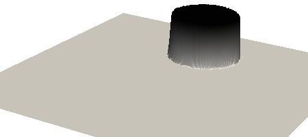
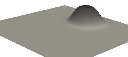
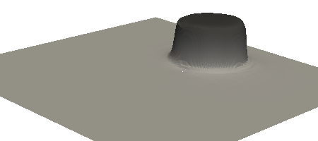
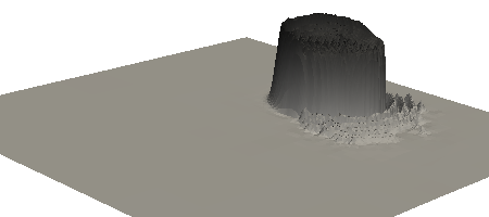
We describe in this section an entropy viscosity technique to stabilize the Galerkin formulation (16). This method has been introduced in Guermond et al. [22] and we refer to Bonito et al. [8] for a mathematical discussion on its stability properties. To motivate the discussion, we refer to the panel (b) of Figure 2 showing the Galerkin approximation of the characteristic function of the unit disk, initially centered at (12,0)120(\frac{1}{2},0), after one rotation about the origin.
Refer to caption
(a)
Refer to caption
(b)
Refer to caption
(c)
Refer to caption
(d)
Figure 2: Graph of the level-set function in the computational domain Λ=(1,1)2Λsuperscript112\Lambda=(-1,1)^{2} using the velocity given by e (49): (a) Initial data: ϕ0subscriptitalic-ϕ0\phi_{0} is the characteristic function of the disk of radius 111 centered at (12,0)120(\frac{1}{2},0); (b) No stabilization; (c) First-order stabilization with CLin=0.1subscript𝐶Lin0.1C_{\text{Lin}}=0.1; (d) Entropy viscosity stabilization with CLin=0.1subscript𝐶Lin0.1C_{\text{Lin}}=0.1 and CEnt=0.1subscript𝐶Ent0.1C_{\text{Ent}}=0.1. Observe the spurious oscillations in panel (b) when no stabilization is applied. Both, the first-order and the entropy viscosity solution are free of oscillations, the latter being clearly more accurate.

The spurious oscillations are avoided by augmenting (16) with an artificial viscosity term where the viscosity is localized and chosen to be proportional to an entropy residual. To describe the method and define an appropriate local “viscosity”, we recall that the following holds in the distribution sense for any E𝒞1(Λ;)𝐸superscript𝒞1ΛE\in{\mathcal{C}}^{1}(\Lambda;\mathbb{R}):

tE(ϕ)+𝐮E(ϕ)λsign(ϕ)(𝒢(Φ)ϕ2)E(ϕ)=0,𝑡𝐸italic-ϕ𝐮𝐸italic-ϕ𝜆signitalic-ϕ𝒢Φsubscriptnormitalic-ϕsuperscript2superscript𝐸italic-ϕ0\dfrac{\partial}{\partial t}E(\phi)+{\bf u}{\cdot}\nabla E(\phi)-\lambda\mbox{sign}(\phi)\left(\mathcal{G}(\Phi)-\|\nabla\phi\|_{\ell^{2}}\right)E^{\prime}(\phi)=0,

Consequently, it is reasonable to expect that the semi-discrete entropy residual

REnt(Φ,𝐮):=tE(Φ)+𝐮(t)E(Φ)λsign(Φ)(𝒢(Φ)Φ2)E(Φ)bassignsuperscript𝑅EntΦ𝐮𝑡𝐸Φ𝐮𝑡𝐸Φ𝜆signΦ𝒢ΦsubscriptnormΦsuperscript2superscript𝐸Φ𝑏R^{\mathrm{Ent}}(\Phi,{\bf u}):=\dfrac{\partial}{\partial t}E(\Phi)+{\bf u}(t){\cdot}\nabla E(\Phi)-\lambda\mbox{sign}(\Phi)\left(\mathcal{G}(\Phi)-\|\nabla\Phi\|_{\ell^{2}}\right)E^{\prime}(\Phi)b

is a reliable indicator of the regularity of ϕitalic-ϕ\phi. This quantity should be of the order of the consistency error in the regions where ϕitalic-ϕ\phi is smooth and it should be large in the region where the PDE is not well solved. In our computations, we have chosen

E(ϕ)=|ϕ|p,𝐸italic-ϕsuperscriptitalic-ϕ𝑝E(\phi)=|\phi|^{p}, (17)

The local so-called entropy viscosity is defined for any K𝒯𝐾𝒯K\in\mathcal{T} by

μKEnt(Φ,𝐮):=CEnthK2REnt(Φ,𝐮)L(K)E(Φ)1|Λ|ΛE(Φ)L(Λ),assignsubscriptsuperscript𝜇Ent𝐾Φ𝐮subscript𝐶Entsuperscriptsubscript𝐾2subscriptnormsuperscript𝑅EntΦ𝐮superscript𝐿𝐾subscriptnorm𝐸Φ1ΛsubscriptΛ𝐸Φsuperscript𝐿Λ{\mu}^{\text{Ent}}_{K}(\Phi,{\bf u}):=C_{\text{Ent}}h_{K}^{2}\frac{\|R^{\text{Ent}}(\Phi,{\bf u})\|_{L^{\infty}(K)}}{\|E(\Phi)-\frac{1}{|\Lambda|}\int_{\Lambda}E(\Phi)\|_{L^{\infty}(\Lambda)}}, (18)

where CEntsubscript𝐶EntC_{\text{Ent}} is an absolute constant. In the regions where ϕitalic-ϕ\phi is discontinuous (or has a very sharp gradient), the entropy viscosity as defined above may be too large and thereby introduce too much diffusion, which in turn may severely limit the CFL number when using an explicit time stepping. In this case a linear first-order viscosity is turned on instead

μKLin(Φ,𝐮)=CLinhK(𝐮+λsign(Φ)ΦΦ2)L(K),subscriptsuperscript𝜇Lin𝐾Φ𝐮subscript𝐶Linsubscriptnormsubscript𝐾𝐮𝜆signΦΦsubscriptnormΦsuperscript2superscript𝐿𝐾\mu^{\text{Lin}}_{K}(\Phi,{\bf u})=C_{\text{Lin}}\|h_{K}({{\bf u}}+\lambda\mbox{sign}(\Phi)\frac{\nabla\Phi}{\|\nabla\Phi\|_{\ell^{2}}})\|_{L^{\infty}(K)}, (19)

where CLinsubscript𝐶LinC_{\text{Lin}} is an absolute constant. The justification for the definition of the local speed that is used to define the viscosity in (19) is that (10) can be re-written tϕ+𝐰ϕ=λsign(ϕ)𝒢(ϕ)𝑡italic-ϕ𝐰italic-ϕ𝜆signitalic-ϕ𝒢italic-ϕ\frac{\partial}{\partial{t}}{\phi}+{\bf w}{\cdot}\nabla\phi=\lambda\mbox{sign}(\phi)\mathcal{G}(\phi), where 𝐰=𝐮+λsign(ϕ)ϕϕ2𝐰𝐮𝜆signitalic-ϕitalic-ϕsubscriptnormitalic-ϕsuperscript2{\bf w}={\bf u}+\lambda\mbox{sign}(\phi)\frac{\nabla\phi}{\|\nabla\phi\|_{\ell^{2}}}. Combining the two viscosities yield the artificial viscosity μStab:Λ×[0,T]:superscript𝜇StabΛ0𝑇\mu^{\text{Stab}}:\Lambda{\times}[0,T]\rightarrow\mathbb{R} defined on each K𝒯𝐾𝒯K\in\mathcal{T} by

μStab(Φ,𝐮)|K:=min(μKLin(Φ,𝐮),μKEnt(Φ,𝐮)).assignevaluated-atsuperscript𝜇StabΦ𝐮𝐾subscriptsuperscript𝜇Lin𝐾Φ𝐮subscriptsuperscript𝜇Ent𝐾Φ𝐮{\mu}^{\text{Stab}}(\Phi,{\bf u})|_{K}:=\min({\mu}^{\text{Lin}}_{K}(\Phi,{\bf u}),\mu^{\text{Ent}}_{K}(\Phi,{\bf u})). (20)

Going back to the space discretization, we modify (16) as follows: Look for Φ𝒞1([0,T];𝕎L(𝒯))Φsuperscript𝒞10𝑇subscript𝕎𝐿𝒯\Phi\in\mathcal{C}^{1}([0,T];\mathbb{W}_{L}(\mathcal{T})) so that

ΛtΦW=Λ𝐮ΦW+Λλsign(Φ)(𝒢(Φ)Φ2)WΛμStab(Φ,𝐮)ΦWsubscriptΛ𝑡Φ𝑊subscriptΛ𝐮Φ𝑊subscriptΛ𝜆signΦ𝒢ΦsubscriptnormΦsuperscript2𝑊subscriptΛsuperscript𝜇StabΦ𝐮Φ𝑊\int_{\Lambda}\dfrac{\partial}{\partial{t}}\Phi W=-\int_{\Lambda}{\bf u}{\cdot}\nabla\Phi\,W+\int_{\Lambda}\lambda\text{sign}(\Phi)\left(\mathcal{G}(\Phi)-\|\nabla\Phi\|_{\ell^{2}}\right)W-\int_{\Lambda}{\mu}^{\text{Stab}}(\Phi,{\bf u})\nabla\Phi{\cdot}\nabla W (21)

for all W𝕎0(𝒯)𝑊subscript𝕎0𝒯W\in\mathbb{W}_{0}(\mathcal{T}) and Φ(,0)=Φ0Φ0subscriptΦ0\Phi(\cdot,0)=\Phi_{0}.

3.1.3 Approximation in Time

Before introducing the time discretization we re-write (21) as follows:

ΛtΦW=ΛL(Φ,𝐮)WΛμStab(Φ,𝐮)ΦW,W𝕎0(𝒯,t),formulae-sequencesubscriptΛ𝑡Φ𝑊subscriptΛ𝐿Φ𝐮𝑊subscriptΛsuperscript𝜇StabΦ𝐮Φ𝑊for-all𝑊subscript𝕎0𝒯𝑡\int_{\Lambda}\dfrac{\partial}{\partial t}\Phi\,W=\int_{\Lambda}L(\Phi,{\bf u})W-\int_{\Lambda}\mu^{\textrm{Stab}}(\Phi,{\bf u})\nabla\Phi{\cdot}\nabla W,\qquad\forall W\in\mathbb{W}_{0}(\mathcal{T},t), (22)

where L(Φ,𝐮):=𝐮+λsign(Φ)(𝒢(Φ)Φ2)assign𝐿Φ𝐮𝐮𝜆signΦ𝒢ΦsubscriptnormΦsuperscript2L(\Phi,{\bf u}):=-{\bf u}+\lambda\text{sign}(\Phi)\left(\mathcal{G}(\Phi)-\|\nabla\Phi\|_{\ell^{2}}\right). Then we approximate time in the above nonlinear system of ODES by using an explicit RK3 strong stability preserving (SSP) scheme, e.g. see Gottlieb et al. [18], Shu and Osher [29] for more details on SSP methods. We denote by ΦksuperscriptΦ𝑘\Phi^{k} the approximation of Φ(,tk)Φsuperscript𝑡𝑘\Phi(\cdot,t^{k}), 0kN0𝑘𝑁0\leq k\leq N. Then, the time stepping proceeds as follows: Given ΦnsuperscriptΦ𝑛\Phi^{n}, compute Φ1superscriptΦ1\Phi^{1}, Φ2,Φ3W(𝒯)superscriptΦ2superscriptΦ3𝑊𝒯\Phi^{2},\Phi^{3}\in W(\mathcal{T}) and Φn+1𝕎L(𝒯)superscriptΦ𝑛1subscript𝕎𝐿𝒯\Phi^{n+1}\in\mathbb{W}_{L}(\mathcal{T}) so that

(i)𝑖\displaystyle(i)\qquad ΛΦ(1)W=Λ(Φn+δtn+1L(Φn,𝐮n))W,W𝕎(𝒯)formulae-sequencesubscriptΛsuperscriptΦ1𝑊subscriptΛsuperscriptΦ𝑛𝛿superscript𝑡𝑛1𝐿superscriptΦ𝑛superscript𝐮𝑛𝑊for-all𝑊𝕎𝒯\displaystyle\int_{\Lambda}\Phi^{(1)}\,W=\int_{\Lambda}\left(\Phi^{n}\ +\delta t^{n+1}L(\Phi^{n},{\bf u}^{n})\right)W,\qquad\forall W\in\mathbb{W}(\mathcal{T})
(ii)𝑖𝑖\displaystyle(ii)\qquad ΛΦ(2)W=Λ(34Φn+14Φ(1)+14δtn+1L(Φ(1),𝐮n+1))WΛμStab,n+1Φ(1)W,W𝕎(𝒯)formulae-sequencesubscriptΛsuperscriptΦ2𝑊subscriptΛ34superscriptΦ𝑛14superscriptΦ114𝛿superscript𝑡𝑛1𝐿superscriptΦ1superscript𝐮𝑛1𝑊subscriptΛsuperscript𝜇Stab𝑛1superscriptΦ1𝑊for-all𝑊𝕎𝒯\displaystyle\int_{\Lambda}\Phi^{(2)}\,W=\int_{\Lambda}\left(\dfrac{3}{4}\Phi^{n}+\dfrac{1}{4}\Phi^{(1)}+\dfrac{1}{4}\delta t^{n+1}L(\Phi^{(1)},{\bf u}^{n+1})\right)W-\int_{\Lambda}\mu^{\mathrm{Stab},n+1}\nabla\Phi^{(1)}{\cdot}\nabla W,\qquad\forall W\in\mathbb{W}(\mathcal{T}) (23)
(iii)𝑖𝑖𝑖\displaystyle(iii)\qquad ΛΦ(3)W=Λ(13Φn+23Φ(2)+23δtn+1L(Φ(2),𝐮n+12))WΛμStab,n+12Φ(2)W,W𝕎(𝒯)formulae-sequencesubscriptΛsuperscriptΦ3𝑊subscriptΛ13superscriptΦ𝑛23superscriptΦ223𝛿superscript𝑡𝑛1𝐿superscriptΦ2superscript𝐮𝑛12𝑊subscriptΛsuperscript𝜇Stab𝑛12superscriptΦ2𝑊for-all𝑊𝕎𝒯\displaystyle\int_{\Lambda}\Phi^{(3)}\,W=\int_{\Lambda}\left(\dfrac{1}{3}\Phi^{n}+\dfrac{2}{3}\Phi^{(2)}+\dfrac{2}{3}\delta t^{n+1}L(\Phi^{(2)},{\bf u}^{n+\frac{1}{2}})\right)W-\int_{\Lambda}\mu^{\mathrm{Stab},n+\frac{1}{2}}\nabla\Phi^{(2)}{\cdot}\nabla W,\qquad\forall W\in\mathbb{W}(\mathcal{T})

and

Φn+1(𝐱,t)={Φ(3)(𝐱)when 𝐱ΓL,ΦL(𝐱,tn+1)when 𝐱ΓL.superscriptΦ𝑛1𝐱𝑡casessuperscriptΦ3𝐱when 𝐱subscriptΓ𝐿subscriptΦ𝐿𝐱superscript𝑡𝑛1when 𝐱subscriptΓ𝐿\Phi^{n+1}({\bf x},t)=\left\{\begin{array}[]{ll}\Phi^{(3)}({\bf x})&\quad\textrm{when }{\bf x}\not\in\Gamma_{L},\\ \Phi_{L}({\bf x},t^{n+1})&\quad\textrm{when }{\bf x}\in\Gamma_{L}.\end{array}\right. (24)

Using (20), the viscosities μStab,n+1superscript𝜇Stab𝑛1\mu^{\mathrm{Stab},n+1} and μStab,n+12superscript𝜇Stab𝑛12\mu^{\mathrm{Stab},n+\frac{1}{2}} are defined to be equal to μStab(Φ(1),𝐮n+1)superscript𝜇StabsuperscriptΦ1superscript𝐮𝑛1\mu^{\textrm{Stab}}(\Phi^{(1)},{\bf u}^{n+1}) and μStab(Φ(2),𝐮n+12)superscript𝜇StabsuperscriptΦ2superscript𝐮𝑛12\mu^{\textrm{Stab}}(\Phi^{(2)},{\bf u}^{n+\frac{1}{2}}), respectively, where the residual REntsuperscript𝑅EntR^{\textrm{Ent}} in the definition (18) of μEntsuperscript𝜇Ent\mu^{\textrm{Ent}} is evaluated as follows:

R(Φ(1),𝐮n+1)𝑅superscriptΦ1superscript𝐮𝑛1\displaystyle R(\Phi^{(1)},{\bf u}^{n+1}) E(Φ(1))E(Φn)δtn+1+(𝐮(tn+1)Φ(1)λsign(Φ(1))(𝒢(Φ(1))Φ(1)2))E(Φ(1))absent𝐸superscriptΦ1𝐸superscriptΦ𝑛𝛿superscript𝑡𝑛1𝐮superscript𝑡𝑛1superscriptΦ1𝜆signsuperscriptΦ1𝒢superscriptΦ1subscriptnormsuperscriptΦ1superscript2superscript𝐸superscriptΦ1\displaystyle\approx\frac{E(\Phi^{(1)})-E(\Phi^{n})}{\delta t^{n+1}}+\left({\bf u}(t^{n+1}){\cdot}\nabla\Phi^{(1)}-\lambda\mbox{sign}(\Phi^{(1)})\left(\mathcal{G}(\Phi^{(1)})-\|\nabla\Phi^{(1)}\|_{\ell^{2}}\right)\right)E^{\prime}(\Phi^{(1)}) (25)
R(Φ(2),𝐮n+12)𝑅superscriptΦ2superscript𝐮𝑛12\displaystyle R(\Phi^{(2)},{\bf u}^{n+\frac{1}{2}}) E(Φ(2))E(Φn)12δtn+1+(𝐮(tn+12)Φ(2)λsign(Φ(2))(𝒢(Φ(2))Φ(2)2))E(Φ(2)).absent𝐸superscriptΦ2𝐸superscriptΦ𝑛12𝛿superscript𝑡𝑛1𝐮superscript𝑡𝑛12superscriptΦ2𝜆signsuperscriptΦ2𝒢superscriptΦ2subscriptnormsuperscriptΦ2superscript2superscript𝐸superscriptΦ2\displaystyle\approx\frac{E(\Phi^{(2)})-E(\Phi^{n})}{\frac{1}{2}\delta t^{n+1}}+\left({\bf u}(t^{n+\frac{1}{2}}){\cdot}\nabla\Phi^{(2)}-\lambda\mbox{sign}(\Phi^{(2)})\left(\mathcal{G}(\Phi^{(2)})-\|\nabla\Phi^{(2)}\|_{\ell^{2}}\right)\right)E^{\prime}(\Phi^{(2)}). (26)
Remark 1 (“On the Fly” Stabilization).

Notice that following Bonito et al. [8], no viscosity is added in the computation of Φ(1)superscriptΦ1\Phi^{(1)}. In particular, the viscosities used within the time interval [tn,tn+1]superscript𝑡𝑛superscript𝑡𝑛1[t^{n},t^{n+1}] only depend on the values of ΦΦ\Phi and 𝐮𝐮{\bf u} on the same time interval.

Remark 2 (Stability and Convergence).

We expect the scheme to be stable under the following Courant-Friedrichs-Lewy (CFL) condition:

δtn+1CCFLminK𝒯hK𝐮(tn+1)+λsign(Φn)ΦnΦn2L(K),𝛿superscript𝑡𝑛1subscript𝐶𝐶𝐹𝐿subscript𝐾𝒯subscript𝐾subscriptnorm𝐮superscript𝑡𝑛1𝜆signsuperscriptΦ𝑛superscriptΦ𝑛subscriptnormsuperscriptΦ𝑛superscript2superscript𝐿𝐾\delta t^{n+1}\leq C_{CFL}\min_{K\in\mathcal{T}}\frac{h_{K}}{\|{\bf u}(t^{n+1})+\lambda\mbox{\rm sign}(\Phi^{n})\frac{\nabla\Phi^{n}}{\|\nabla\Phi^{n}\|_{\ell^{2}}}\ \|_{L^{\infty}(K)}}, (27)

for some sufficiently small but positive constant CCFLsubscript𝐶𝐶𝐹𝐿C_{CFL} independent of λ𝜆\lambda, 𝒯𝒯\mathcal{T}, δt𝛿𝑡\delta t, ΦΦ\Phi and 𝐮𝐮{\bf u}. Refer for instance to Bonito et al. [8] for further details on the CFL condition. Moreover, it seems reasonable to expect that only the entropy viscosity is active in the regions where ϕitalic-ϕ\phi is smooth; as a result, the CFL condition implies that the first-order approximation of the time derivative in the evaluation of the entropy residuals, (25)-(26), does not affect the overall third-order approximation thanks to the hK2superscriptsubscript𝐾2h_{K}^{2} factor present in the definition of the viscosity (18). This conjecture is confirmed numerically in Section 4.2.

3.2 Numerical Approximation of The Navier-Stokes System

The space approximation of the velocity and pressure in the Navier-Stokes equations is done by using Taylor-Hood finite elements. The time discretization is done by using the second-order backward differentiation formula (BDF2). An incremental rotational pressure correction scheme is adopted to uncouple the velocity and the pressure. We refer to Guermond and Shen [20] for the convergence analysis of the metod and to Guermond et al. [21] for a review on projection methods.

3.2.1 The Space Discretization

Let 𝐅Dsubscript𝐅𝐷{\bf F}_{D} be a continuous, piecewise quadratic approximation of 𝐟Dsubscript𝐟𝐷{\bf f}_{D} on ΓDsubscriptΓ𝐷\Gamma_{D}. The finite element discretization of the velocity and the pressure is done by using the following linear and affine spaces:

𝕍0(𝒯)subscript𝕍0𝒯\displaystyle\boldsymbol{\mathbb{V}}_{0}(\mathcal{T}) :={𝐕C0(Λ¯;d)|𝐕|ΓD=0,𝐕𝝂|ΓS=0,𝐕|K2(K),K𝒯},assignabsentconditional-set𝐕superscript𝐶0¯Λsuperscript𝑑formulae-sequenceevaluated-at𝐕subscriptΓ𝐷0formulae-sequenceevaluated-at𝐕𝝂subscriptΓ𝑆0formulae-sequenceevaluated-at𝐕𝐾superscript2𝐾for-all𝐾𝒯\displaystyle:=\{{\bf V}\in C^{0}({\overline{\Lambda}};\mathbb{R}^{d})\ |\ {\bf V}{|_{\Gamma_{D}}}=0,\ {\bf V}{\cdot}{\boldsymbol{\nu}}|_{\Gamma_{S}}=0,\ {\bf V}|_{K}\in\boldsymbol{\mathbb{Q}}^{2}(K),\ \forall K\in\mathcal{T}\}, (28)
𝕍D(𝒯)subscript𝕍𝐷𝒯\displaystyle\boldsymbol{\mathbb{V}}_{D}(\mathcal{T}) :={𝐕C0(Λ¯;d)|𝐕|ΓD=𝐅D,𝐕𝝂|ΓS=0,𝐕|K2(K),K𝒯},assignabsentconditional-set𝐕superscript𝐶0¯Λsuperscript𝑑formulae-sequenceevaluated-at𝐕subscriptΓ𝐷subscript𝐅𝐷formulae-sequenceevaluated-at𝐕𝝂subscriptΓ𝑆0formulae-sequenceevaluated-at𝐕𝐾superscript2𝐾for-all𝐾𝒯\displaystyle:=\{{\bf V}\in C^{0}({\overline{\Lambda}};\mathbb{R}^{d})\ |\ {\bf V}{|_{\Gamma_{D}}}={\bf F}_{D},\ {\bf V}{\cdot}{\boldsymbol{\nu}}|_{\Gamma_{S}}=0,\ {\bf V}|_{K}\in\boldsymbol{\mathbb{Q}}^{2}(K),\ \forall K\in\mathcal{T}\}, (29)
𝕄(𝒯)𝕄𝒯\displaystyle\mathbb{M}(\mathcal{T}) :={QC0(Λ¯)|Q|K1(K),K𝒯},assignabsentconditional-set𝑄superscript𝐶0¯Λformulae-sequenceevaluated-at𝑄𝐾superscript1𝐾for-all𝐾𝒯\displaystyle:=\{Q\in C^{0}({\overline{\Lambda}})\rightarrow\mathbb{R}\ |\ Q|_{K}\in\mathbb{Q}^{1}(K),\ \forall K\in\mathcal{T}\}, (30)

Upon setting 𝐔(0)=𝐔0𝐔0subscript𝐔0{\bf U}(0)={\bf U}_{0}, where 𝐔0subscript𝐔0{\bf U}_{0} is a continuous, piecewise quadratic approximation of the initial velocity 𝐮0subscript𝐮0{\bf u}_{0} in 𝕍D(𝒯)subscript𝕍𝐷𝒯\boldsymbol{\mathbb{V}}_{D}(\mathcal{T}), the semi-discrete formulation of (1) consists of looking for 𝐔𝒞1([0,T];𝕍D(𝒯))𝐔superscript𝒞10𝑇subscript𝕍𝐷𝒯{\bf U}\in\mathcal{C}^{1}([0,T];\boldsymbol{\mathbb{V}}_{D}(\mathcal{T})) and P𝒞0([0,T];𝕄(𝒯)P\in\mathcal{C}^{0}([0,T];\mathbb{M}(\mathcal{T}) such that the following holds for every t(0,T]𝑡0𝑇t\in(0,T]:

Λρ(t𝐔+(𝐔)𝐔)𝐕+2Λμ(S𝐔:S𝐕)ΛPdiv𝐕+ΛQdiv𝐔=Λρ𝐠𝐕+ΓN𝐟N𝐕+Σ(t)σκ𝐧𝐕,(𝐕,Q)𝕍0(𝒯)×𝕄(𝒯),\begin{split}\int_{\Lambda}\rho\left(\dfrac{\partial}{\partial t}{\bf U}+({\bf U}{\cdot}\nabla){\bf U}\right){\cdot}{\bf V}+2\int_{\Lambda}\mu\left(\nabla^{S}{\bf U}{:}\nabla^{S}{\bf V}\right)-\int_{\Lambda}P\text{div}{\bf V}+\int_{\Lambda}Q\,\text{div}{\bf U}\\ =\int_{\Lambda}\rho{{\bf g}}{\cdot}{\bf V}+\int_{\Gamma_{N}}{\bf f}_{N}{\cdot}{\bf V}+\int_{\Sigma(t)}\sigma\kappa\,{\bf n}{\cdot}{\bf V},\qquad\forall({\bf V},Q)\in\mathbb{V}_{0}(\mathcal{T}){\times}\mathbb{M}(\mathcal{T}),\end{split} (31)

3.2.2 Time discretization

The time discretization of (31) is done by using the second-order backward differentiation formula (BDF2) and an incremental pressure correction scheme in rotational form introduced and studied in Guermond and Salgado [19] to decouple the velocity and the pressure. In addition to the approximation of the initial condition 𝐔0superscript𝐔0{{\bf U}}^{0} mentioned above, the algorithm requires an approximation P0𝕄(𝒯)subscript𝑃0𝕄𝒯P_{0}\in\mathbb{M}(\mathcal{T}) of the initial pressure p(0)𝑝0p(0). We denote by 𝐔nsuperscript𝐔𝑛{\bf U}^{n}, Pnsuperscript𝑃𝑛P^{n} and ΨnsuperscriptΨ𝑛\Psi^{n} the approximations of 𝐔(,tn)𝐔superscript𝑡𝑛{\bf U}(\cdot,t^{n}) and P(,tn)𝑃superscript𝑡𝑛P(\cdot,t^{n}) and the pressure correction, respectively.

The initialization step consists of setting: 𝐔0=𝐔0superscript𝐔0subscript𝐔0{\bf U}^{0}={\bf U}_{0}, P1=P0=P0superscript𝑃1superscript𝑃0subscript𝑃0P^{-1}=P^{0}=P_{0} and Ψ0=0superscriptΨ00\Psi^{0}=0. Then, given a new time step δtn+1𝛿superscript𝑡𝑛1\delta t^{n+1}, given 𝐔n𝕍D(𝒯)superscript𝐔𝑛subscript𝕍𝐷𝒯{\bf U}^{n}\in\boldsymbol{\mathbb{V}}_{D}(\mathcal{T}), Ψn𝕄(𝒯)superscriptΨ𝑛𝕄𝒯\Psi^{n}\in\mathbb{M}(\mathcal{T}) and Pn𝕄(𝒯)superscript𝑃𝑛𝕄𝒯P^{n}\in\mathbb{M}(\mathcal{T}), and assuming for the time being that ρ(tn+1)𝜌superscript𝑡𝑛1\rho(t^{n+1}), μ(tn+1)𝜇superscript𝑡𝑛1\mu(t^{n+1}) and Σ(tn+1)Σsuperscript𝑡𝑛1\Sigma(t^{n+1}) are also known (see §3.4), the new fields 𝐔n+1𝕍D(𝒯)superscript𝐔𝑛1subscript𝕍𝐷𝒯{\bf U}^{n+1}\in\boldsymbol{\mathbb{V}}_{D}(\mathcal{T}), Ψn+1𝕄(𝒯)superscriptΨ𝑛1𝕄𝒯\Psi^{n+1}\in\mathbb{M}(\mathcal{T}) and Pn+1𝕄(𝒯)superscript𝑃𝑛1𝕄𝒯P^{n+1}\in\mathbb{M}(\mathcal{T}) are computed in three steps:
111 Velocity Prediction: Find 𝐔n+1𝕍D(𝒯)superscript𝐔𝑛1subscript𝕍𝐷𝒯{\bf U}^{n+1}\in\boldsymbol{\mathbb{V}}_{D}(\mathcal{T}) such that

Λρ(tn+1)δBDF2δtn+1𝐔n+1𝐕+2Λμ(tn+1)(S(𝐔n+1):S𝐕)+S𝒯(𝐔n+1,𝐕)=Λρ(tn+1)((𝐔n)𝐔n)𝐕+Λ(Pn+43Ψn13Ψn1)div(𝐕)+Λρn+1𝐠n+1+ΓN𝐟Nn+1𝐕+Σ(tn+1)σκn+1𝐧n+1𝐕,𝐕𝕍0(𝒯),\int_{\Lambda}\rho(t^{n+1})\frac{\delta_{\mbox{\tiny BDF2}}}{\delta t^{n+1}}{{\bf U}}^{n+1}{\cdot}{{\bf V}}+2\int_{\Lambda}{\mu(t^{n+1})}\left(\nabla^{S}({{\bf U}}^{n+1}){:}\nabla^{S}{{\bf V}}\right)+S_{\mathcal{T}}({\bf U}^{n+1},{\bf V})\\ =-\int_{\Lambda}\rho(t^{n+1})(({{\bf U}}^{n})^{\star}{\cdot}\nabla{{\bf U}}^{n}){\cdot}{{\bf V}}+\int_{\Lambda}(P^{n}+\dfrac{4}{3}\Psi^{n}-\dfrac{1}{3}\Psi^{n-1})\mbox{div}({{\bf V}})\\ +\int_{\Lambda}\rho^{n+1}{{\bf g}^{n+1}}+\int_{\Gamma_{N}}{\bf f}_{N}^{n+1}{\cdot}{\bf V}+\int_{\Sigma(t^{n+1})}\sigma\kappa^{n+1}\,{\bf n}^{n+1}{\cdot}{\bf V},\quad\forall{\bf V}\in\boldsymbol{\mathbb{V}}_{0}(\mathcal{T}), (32)

where

  • 1.

    the BDF2 approximation of the time derivative with variable time stepping is given by

    t𝐔(𝐱,tn+1)δBDF2δtn+1𝐔n+1(𝐱):=1δtn+1(1+2ηn+11+ηn+1𝐔n+1(𝐱)(1+ηn+1)𝐔n(𝐱)+ηn+121+ηn+1𝐔n1(𝐱)),ηl+1:=δtl+1δtl;formulae-sequence𝑡𝐔𝐱superscript𝑡𝑛1subscript𝛿BDF2𝛿superscript𝑡𝑛1superscript𝐔𝑛1𝐱assign1𝛿superscript𝑡𝑛112subscript𝜂𝑛11subscript𝜂𝑛1superscript𝐔𝑛1𝐱1subscript𝜂𝑛1superscript𝐔𝑛𝐱subscriptsuperscript𝜂2𝑛11subscript𝜂𝑛1superscript𝐔𝑛1𝐱assignsubscript𝜂𝑙1𝛿superscript𝑡𝑙1𝛿superscript𝑡𝑙\dfrac{\partial}{\partial t}{\bf U}({\bf x},t^{n+1})\approx\frac{\delta_{\mbox{\tiny BDF2}}}{\delta t^{n+1}}{\bf U}^{n+1}({\bf x}):=\dfrac{1}{\delta t^{n+1}}\left(\dfrac{1+2\eta_{n+1}}{1+\eta_{n+1}}{\bf U}^{n+1}({\bf x})-(1+\eta_{n+1}){\bf U}^{n}({\bf x})+\dfrac{\eta^{2}_{n+1}}{1+\eta_{n+1}}{\bf U}^{n-1}({\bf x})\right),\qquad\eta_{l+1}:=\frac{\delta t^{l+1}}{\delta t^{l}};
  • 2.

    the extrapolated velocity (𝐔n)superscriptsuperscript𝐔𝑛({\bf U}^{n})^{\star} is defined by (𝐔n):=𝐔n+ηn(𝐔n𝐔n1)assignsuperscriptsuperscript𝐔𝑛superscript𝐔𝑛superscript𝜂𝑛superscript𝐔𝑛superscript𝐔𝑛1({\bf U}^{n})^{\star}:={\bf U}^{n}+\eta^{n}({\bf U}^{n}-{\bf U}^{n-1});

  • 3.

    as discussed in Bonito et al. [9], the bilinear form S𝒯:𝕍(𝒯)×𝕍(𝒯):subscript𝑆𝒯𝕍𝒯𝕍𝒯S_{\mathcal{T}}:\mathbb{V}(\mathcal{T}){\times}\mathbb{V}(\mathcal{T})\rightarrow\mathbb{R} is added to control the divergence of the velocity and to cope with variable time stepping and open boundary conditions

    S𝒯(𝐖,𝐕):=CstabK𝒯K(μn+1+ρn+1hK𝐖L(K))(𝐖)(𝐕),assignsubscript𝑆𝒯𝐖𝐕subscript𝐶stabsubscript𝐾𝒯subscript𝐾superscript𝜇𝑛1superscript𝜌𝑛1subscriptnormsubscript𝐾𝐖superscript𝐿𝐾𝐖𝐕S_{\mathcal{T}}({\bf W},{\bf V}):=C_{\text{stab}}\sum_{K\in\mathcal{T}}\int_{K}(\mu^{n+1}+\rho^{n+1}\|h_{K}{\bf W}\|_{L^{\infty}({K})})(\nabla{\cdot}{\bf W})(\nabla{\cdot}{\bf V}), (33)

    where Cstabsubscript𝐶stabC_{\text{stab}} is an absolute constant.

222 Pressure Correction Step: The pressure increment Ψn+1𝕄(𝒯)superscriptΨ𝑛1𝕄𝒯\Psi^{n+1}\in\mathbb{M}(\mathcal{T}) is determined by solving

ΛΨn+1Q=3minxΛρ(tn+1)2δtn+1Λdiv(𝐔n+1)Q,Q𝕄(𝒯).formulae-sequencesubscriptΛsuperscriptΨ𝑛1𝑄3subscript𝑥Λ𝜌superscript𝑡𝑛12𝛿superscript𝑡𝑛1subscriptΛdivsuperscript𝐔𝑛1𝑄for-all𝑄𝕄𝒯\int_{\Lambda}\nabla\Psi^{n+1}\nabla Q=-\dfrac{3\min_{x\in\Lambda}\rho(t^{n+1})}{2\delta t^{n+1}}\int_{\Lambda}\text{div}({{\bf U}}^{n+1})Q,\ \ \ \forall Q\in\mathbb{M}(\mathcal{T}). (34)

333 Pressure Update: The pressure Pn+1𝕄(𝒯)superscript𝑃𝑛1𝕄𝒯P^{n+1}\in\mathbb{M}(\mathcal{T}) is obtained by solving

ΛPn+1Q=Λ(Pn+Ψn+1)QminxΛμ(tn+1)Λdiv(𝐔n+1)Q,Q𝕄(𝒯).formulae-sequencesubscriptΛsuperscript𝑃𝑛1𝑄subscriptΛsuperscript𝑃𝑛superscriptΨ𝑛1𝑄subscript𝑥Λ𝜇superscript𝑡𝑛1subscriptΛdivsuperscript𝐔𝑛1𝑄for-all𝑄𝕄𝒯\int_{\Lambda}P^{n+1}Q=\int_{\Lambda}\left(P^{n}+\Psi^{n+1}\right)Q-\min_{x\in\Lambda}\mu(t^{n+1})\int_{\Lambda}\mbox{div}({{\bf U}}^{n+1})\,Q,\ \forall Q\in\mathbb{M}(\mathcal{T}). (35)

For stability purposes, we restrict the space and time discretization parameters to satisfy a CFL condition

δtn+1CCFL12minK𝒯hhK𝐔nL(Λ),𝛿superscript𝑡𝑛1subscript𝐶CFL12subscript𝐾subscript𝒯subscript𝐾subscriptnormsuperscript𝐔𝑛superscript𝐿Λ\delta t^{n+1}\leq C_{\textrm{CFL}}\frac{1}{2}\frac{\min_{K\in\mathcal{T}_{h}}h_{K}}{\|{\bf U}^{n}\|_{L^{\infty}(\Lambda)}}, (36)

where CCFLsubscript𝐶CFLC_{\textrm{CFL}} is the same constant appearing in (27) and 12minK𝒯hhK12subscript𝐾subscript𝒯subscript𝐾\frac{1}{2}\min_{K\in\mathcal{T}_{h}}h_{K} is the minimum distance between two Lagrange nodes using 2subscript2{\mathbb{Q}}_{2} elements.

3.3 The Surface Tension

This section describes the approximation of the curvature term Σ(tn+1)σκn+1(𝐧n+1𝐕)subscriptΣsuperscript𝑡𝑛1𝜎superscript𝜅𝑛1superscript𝐧𝑛1𝐕\int_{\Sigma(t^{n+1})}\sigma\kappa^{n+1}\,({\bf n}^{n+1}{\cdot}{\bf V}) appearing in the first step of the projection method (32). We follow the method proposed by Bänsch [4] (see also Hysing et al. [23]) using the work of Dziuk and Elliott [14]. This approach is based on the following representation of total curvature:

κ𝐧=ΣΣ𝐈𝐝Σ,𝜅𝐧subscriptΣsubscriptΣsubscript𝐈𝐝Σ\kappa{\bf n}=\nabla_{\Sigma}{\cdot}\nabla_{\Sigma}\mathrm{\bf Id}_{\Sigma},

where 𝐈𝐝Σsubscript𝐈𝐝Σ\mathrm{\bf Id}_{\Sigma} is the identity mapping on ΣΣ\Sigma and, given any extension 𝐯~~𝐯\tilde{\bf v} of 𝐯𝐯{\bf v} in a neighborhood of ΣΣ\Sigma, the tangential gradient of 𝐯:Σd:𝐯Σsuperscript𝑑{\bf v}:\Sigma\rightarrow\mathbb{R}^{d} is defined by Σ𝐯:=𝐯~|Σ(I𝐧𝐧)assignsubscriptΣ𝐯evaluated-at~𝐯ΣItensor-product𝐧𝐧\nabla_{\Sigma}{\bf v}:=\nabla{\tilde{{\bf v}}}|_{\Sigma}(\text{{\bf I}}-{{\bf n}}\otimes{{\bf n}}), see e.g. Gilbarg and Trudinger [17]. Multipliying the above identity by a test function 𝐕𝐕{\bf V} and integrating by parts over ΣΣ\Sigma yields

Σσκ𝐧𝐕=ΣσΣ𝐈𝐝Σ:Σ𝐕+Σσ𝝉𝐈𝐝Σ𝐕,:subscriptΣ𝜎𝜅𝐧𝐕subscriptΣ𝜎subscriptΣsubscript𝐈𝐝ΣsubscriptΣ𝐕subscriptΣ𝜎subscript𝝉subscript𝐈𝐝Σ𝐕\int_{\Sigma}\sigma\kappa{{\bf n}}{\cdot}{{\bf V}}=-\int_{\Sigma}\sigma{\nabla}_{\Sigma}\mathrm{\bf Id}_{\Sigma}:{\nabla}_{\Sigma}{{\bf V}}+\int_{\partial\Sigma}\sigma\partial_{\boldsymbol{\tau}}\mathrm{\bf Id}_{\Sigma}{\cdot}{\bf V}, (37)

where 𝝉𝝉{\boldsymbol{\tau}} is the co-normal to ΣΣ\Sigma and 𝝉subscript𝝉\partial_{{\boldsymbol{\tau}}} is the derivative in the co-normal direction. In the present context the integral on ΣΣ\partial\Sigma vanishes since either ΣΣ\Sigma is a closed manifold or 𝝉𝐈𝐝Σ=0subscript𝝉subscript𝐈𝐝Σ0\partial_{\boldsymbol{\tau}}\mathrm{\bf Id}_{\Sigma}=0. This identity together with the first-order prediction 𝐈𝐝Σ(tn+1)𝐈𝐝Σ(tn)+δtn+1𝐔n+1subscript𝐈𝐝Σsuperscript𝑡𝑛1subscript𝐈𝐝Σsuperscript𝑡𝑛𝛿superscript𝑡𝑛1superscript𝐔𝑛1\mathrm{\bf Id}_{\Sigma(t^{n+1})}\approx\mathrm{\bf Id}_{\Sigma(t^{n})}+\delta t^{n+1}{\bf U}^{n+1} of the interface evolution (5) gives a semi-implicit representation of the total curvature

Σ(tn+1)σκn+1(𝐧n+1𝐕)subscriptΣsuperscript𝑡𝑛1𝜎superscript𝜅𝑛1superscript𝐧𝑛1𝐕\displaystyle\int_{\Sigma(t^{n+1})}\sigma\kappa^{n+1}\,({\bf n}^{n+1}{\cdot}{\bf V}) =Σ(tn+1)Σ(tn+1)𝐈𝐝Σ(tn+1):Σ(tn+1)𝐕:absentsubscriptΣsuperscript𝑡𝑛1subscriptΣsuperscript𝑡𝑛1subscript𝐈𝐝Σsuperscript𝑡𝑛1subscriptΣsuperscript𝑡𝑛1𝐕\displaystyle=-\int_{\Sigma(t^{n+1})}{\nabla}_{\Sigma(t^{n+1})}\mathrm{\bf Id}_{\Sigma(t^{n+1})}{:}{\nabla}_{\Sigma(t^{n+1})}{{\bf V}}
Σ(tn+1)Σ(tn+1)𝐈𝐝Σ(tn+1):Σ(tn+1)𝐕δtn+1Σ(tn+1)σΣ(tn+1)𝐔n+1:Σ(tn+1)𝐕.:absentsubscriptΣsuperscript𝑡𝑛1subscriptΣsuperscript𝑡𝑛1subscript𝐈𝐝Σsuperscript𝑡𝑛1subscriptΣsuperscript𝑡𝑛1𝐕𝛿superscript𝑡𝑛1subscriptΣsuperscript𝑡𝑛1𝜎subscriptΣsuperscript𝑡𝑛1superscript𝐔𝑛1:subscriptΣsuperscript𝑡𝑛1𝐕\displaystyle\approx-\int_{\Sigma(t^{n+1})}{\nabla}_{\Sigma(t^{n+1})}\mathrm{\bf Id}_{\Sigma(t^{n+1})}{:}{\nabla}_{\Sigma(t^{n+1})}{{\bf V}}-\delta t^{n+1}\int_{\Sigma(t^{n+1})}\sigma{\nabla}_{\Sigma(t^{n+1})}{\bf U}^{n+1}{:}{\nabla}_{\Sigma(t^{n+1})}{{\bf V}}.

One key benefit of this representation comes from the additional stabilizing term Σ(tn+1)σΣ(tn+1)𝐔n+1:Σ(tn+1)𝐕:subscriptΣsuperscript𝑡𝑛1𝜎subscriptΣsuperscript𝑡𝑛1superscript𝐔𝑛1subscriptΣsuperscript𝑡𝑛1𝐕\int_{\Sigma(t^{n+1})}\sigma{\nabla}_{\Sigma(t^{n+1})}{\bf U}^{n+1}{:}{\nabla}_{\Sigma(t^{n+1})}{{\bf V}}, which we keep implicit in (32). The technicalities regarding the approximation of this integral using the level set representation are detailed in section 3.4.2, see (45).

3.4 The Coupled System

The two solvers described in Sections 3.1 and 3.2 above are sequentially combined. The flowchart of the resulting free boundary flow solver is shown in Figure 3. The remaining subsections of §3.4 detail the coupling between the two solvers and other implementation technicalities.

Initialization Solve Level-set Solve Velocity Update Pressure Refine Mesh Choose Time Step
Figure 3: Global Algorithm Flowchart.

3.4.1 Data for the Level-Set Solver (3.1.3)-(24)

Following (3.1.3), given ΦnsuperscriptΦ𝑛\Phi^{n}, an approximation of ϕ(tn)italic-ϕsuperscript𝑡𝑛\phi(t^{n}), the approximation Φn+1superscriptΦ𝑛1\Phi^{n+1} of ϕ(tn+1)italic-ϕsuperscript𝑡𝑛1\phi(t^{n+1}) requires the velocities 𝐮(tn),𝐮(tn+12)𝐮superscript𝑡𝑛𝐮superscript𝑡𝑛12{\bf u}(t^{n}),{\bf u}(t^{n+\frac{1}{2}}) and 𝐮(tn+1)𝐮superscript𝑡𝑛1{\bf u}(t^{n+1}). To avoid an implicit coupling between the level-set solver and the Navier-Stokes solver, these quantities are replaced by second-order extrapolations using 𝐔nsuperscript𝐔𝑛{\bf U}^{n} and 𝐔n1superscript𝐔𝑛1{\bf U}^{n-1}:

𝐮(tn)𝐔n,𝐮(tn+12)𝐔n+12δtn+1δtn(𝐔n𝐔n1),and𝐔n+1𝐔n+δtn+1δtn(𝐔n𝐔n1).formulae-sequence𝐮superscript𝑡𝑛superscript𝐔𝑛formulae-sequence𝐮superscript𝑡𝑛12superscript𝐔𝑛12𝛿superscript𝑡𝑛1𝛿superscript𝑡𝑛superscript𝐔𝑛superscript𝐔𝑛1andsuperscript𝐔𝑛1superscript𝐔𝑛𝛿superscript𝑡𝑛1𝛿superscript𝑡𝑛superscript𝐔𝑛superscript𝐔𝑛1{\bf u}(t^{n})\approx{\bf U}^{n},\qquad{\bf u}(t^{n+\frac{1}{2}})\approx{\bf U}^{n}+\frac{1}{2}\frac{\delta t^{n+1}}{\delta t^{n}}({\bf U}^{n}-{\bf U}^{n-1}),\qquad\text{and}\qquad{\bf U}^{n+1}\approx{\bf U}^{n}+\frac{\delta t^{n+1}}{\delta t^{n}}({\bf U}^{n}-{\bf U}^{n-1}).

The sign(.)\mbox{sign}(.) function that is used in the right-hand side of (10) to make sure that ϕ2subscriptnormitalic-ϕsuperscript2\|\nabla\phi\|_{\ell^{2}} is close to 1 in a small neighborhood of ΣΣ\Sigma (i.e., on the fly reinitialization, see discussion following (11)) is redefined and replaced by:

signh(s)={+1if s>βtanh(CS),1if s<βtanh(CS),0otherwise,subscriptsign𝑠cases1if 𝑠𝛽subscript𝐶𝑆1if 𝑠𝛽subscript𝐶𝑆0otherwise,\mbox{sign}_{h}(s)=\left\{\begin{array}[]{ll}+1&\qquad\text{if }s>\beta\tanh(C_{S}),\\ -1&\qquad\text{if }s<-\beta\tanh(C_{S}),\\ 0&\qquad\text{otherwise,}\end{array}\right. (38)

where CSsubscript𝐶𝑆C_{S} is an absolute constant. The thresholding in the above definition of the approximate sign function gives signh(ϕ(𝐱,t))=±1subscriptsignitalic-ϕ𝐱𝑡plus-or-minus1\mbox{sign}_{h}(\phi({\bf x},t))=\pm 1 whenever |ϕ(𝐱,t)|βtanh(CS)italic-ϕ𝐱𝑡𝛽subscript𝐶𝑆\frac{|\phi({\bf x},t)|}{\beta}\geq\tanh(C_{S}), which is compatible with the behavior ϕ(𝐱,t)βtanh(dist(Σ(t),𝐱)β)italic-ϕ𝐱𝑡𝛽distΣ𝑡𝐱𝛽\frac{\phi({\bf x},t)}{\beta}\approx\tanh\left(\frac{\text{dist}(\Sigma(t),{\bf x})}{\beta}\right) that is expected for the level-set function, see (12).

The parameter λ𝜆\lambda (“reinitialization relative speed” in the language of Ville et al. [35]) is defined for t(tn,tn+1]𝑡superscript𝑡𝑛superscript𝑡𝑛1t\in(t^{n},t^{n+1}] by

λ=Cλ𝐔nL(Λ),K𝒯,formulae-sequence𝜆subscript𝐶𝜆subscriptnormsuperscript𝐔𝑛superscript𝐿Λ𝐾𝒯\lambda=C_{\lambda}\|{\bf U}^{n}\|_{L^{\infty}(\Lambda)},\qquad K\in\mathcal{T}, (39)

where Cλsubscript𝐶𝜆C_{\lambda} is an absolute constant. This definition is motivated by the CFL condition (27). We refer to Ville et al. [35] for further details.

3.4.2 Data for the Navier-Stokes Solver

The definitions of the fields 𝐔n+1superscript𝐔𝑛1{\bf U}^{n+1} and Pn+1superscript𝑃𝑛1P^{n+1} in (32)–(35) invoke the values of the density field ρn+1superscript𝜌𝑛1\rho^{n+1} and viscosity field μn+1superscript𝜇𝑛1\mu^{n+1}. Once ϕn+1superscriptitalic-ϕ𝑛1\phi^{n+1} is computed, these quantities are evaluated by using the following definitions

ρn+1superscript𝜌𝑛1\displaystyle\rho^{n+1} =ρ+1+Hh(Φn+1)2+ρ1Hh(Φn+1)2absentsuperscript𝜌1subscript𝐻superscriptΦ𝑛12superscript𝜌1subscript𝐻superscriptΦ𝑛12\displaystyle=\rho^{+}\dfrac{1+H_{h}(\Phi^{n+1})}{2}+\rho^{-}\dfrac{1-H_{h}(\Phi^{n+1})}{2} (40)
μn+1superscript𝜇𝑛1\displaystyle\mu^{n+1} =μ+1+Hh(Φn+1)2+μ1Hh(Φn+1)2,absentsuperscript𝜇1subscript𝐻superscriptΦ𝑛12superscript𝜇1subscript𝐻superscriptΦ𝑛12\displaystyle=\mu^{+}\dfrac{1+H_{h}(\Phi^{n+1})}{2}+\mu^{-}\dfrac{1-H_{h}(\Phi^{n+1})}{2}, (41)

where, ρ±,μ±superscript𝜌plus-or-minussuperscript𝜇plus-or-minus\rho^{\pm},\mu^{\pm} are the density/viscosity in Ω±superscriptΩplus-or-minus\Omega^{\pm}, and Hh(.)H_{h}(.) an approximation of the Heaviside function defined as follows:

Hh(s)={1,if s>βtanh(CH),1,if s<βtanh(CH),sβtanh(CH),otherwise,subscript𝐻𝑠cases1if 𝑠𝛽subscript𝐶𝐻1if 𝑠𝛽subscript𝐶𝐻𝑠𝛽subscript𝐶𝐻otherwiseH_{h}(s)=\left\{{\begin{array}[]{cl}1,&\qquad\text{if }s>\beta\tanh(C_{H}),\\ -1,&\qquad\text{if }s<-\beta\tanh(C_{H}),\\ \dfrac{s}{\beta\tanh(C_{H})},&\qquad\text{otherwise},\end{array}}\right. (42)

where CHsubscript𝐶𝐻C_{H} is an absolute constant, as suggested in Ville et al. [35]. Similarly to what we have done to approximate the sign function, the above regularization is compatible with the behavior ϕ(𝐱,t)βtanh(dist(Σ(t),𝐱)β)italic-ϕ𝐱𝑡𝛽distΣ𝑡𝐱𝛽\frac{\phi({\bf x},t)}{\beta}\approx\tanh\left(\frac{\text{dist}(\Sigma(t),{\bf x})}{\beta}\right) that is expected for the level-set function.

The approximation of the surface tension term in (32) is done by following Hysing et al. [23]. Let ϵ>0italic-ϵ0\epsilon>0, and consider the piecewise linear regularized Dirac measure supported on Σ(tn+1)Σsuperscript𝑡𝑛1\Sigma(t^{n+1}), say δϵsubscript𝛿italic-ϵ\delta_{\epsilon}, defined by

δϵ(𝐱):={1ϵ(1dist(Σ,𝐱)ϵ)if|dist(Σ,𝐱)|<ϵ,0otherwise.assignsubscript𝛿italic-ϵ𝐱cases1italic-ϵ1distΣ𝐱italic-ϵifdistΣ𝐱italic-ϵ0otherwise\delta_{\epsilon}({\bf x}):=\left\{\begin{array}[]{ll}\dfrac{1}{\epsilon}\left(1-\frac{\text{dist}(\Sigma,{\bf x})}{\epsilon}\right)&\qquad\text{if}\quad|\text{dist}(\Sigma,{\bf x})|<\epsilon,\\ 0&\qquad\text{otherwise}.\end{array}\right. (43)

To account for the fact that we do not have access to the distance to the interface ΣΣ\Sigma but rather to an approximation of βtanh(dist(Σ,𝐱)β)𝛽distΣ𝐱𝛽\beta\tanh(\frac{\text{dist}(\Sigma,{\bf x})}{\beta}), see Section 2.2.2, we rescale δϵ(𝐱)subscript𝛿italic-ϵ𝐱\delta_{\epsilon}({\bf x}) as suggested in Engquist et al. [15], Tornberg [33] and consider instead:

δϵ(𝐱,Φ)={1ϵ~(1Φ(𝐱)ϵ~)Φ(𝐱)2,|Φ(𝐱)|<ϵ~:=ϵΦ(𝐱)1Φ(𝐱)20,otherwise,subscript𝛿italic-ϵ𝐱Φcases1~italic-ϵ1Φ𝐱~italic-ϵsubscriptnormΦ𝐱superscript2Φ𝐱~italic-ϵassignitalic-ϵsubscriptnormΦ𝐱superscript1subscriptnormΦ𝐱superscript20otherwise,\delta_{\epsilon}({\bf x},\Phi)=\left\{\begin{array}[]{ll}\dfrac{1}{\tilde{\epsilon}}\left(1-\frac{\Phi({\bf x})}{\tilde{\epsilon}}\right)\|\nabla\Phi({\bf x})\|_{\ell^{2}},&|\Phi({\bf x})|<\tilde{\epsilon}:=\epsilon\frac{\|\nabla\Phi({\bf x})\|_{\ell^{1}}}{\|\nabla\Phi({\bf x})\|_{\ell^{2}}}\\ 0,&\text{otherwise,}\end{array}\right. (44)

where p\|\cdot\|_{\ell^{p}} is the psuperscript𝑝\ell^{p}-norm in dsuperscript𝑑\mathbb{R}^{d}. In practice, we chose ϵ=βtanh(CH)italic-ϵ𝛽subscript𝐶𝐻\epsilon=\beta\tanh(C_{H}) to be consistent with the approximation of the Heaviside function, see (42). Using this approximate Dirac measure, the approximation of the surface tension discussed in Section 3.3 becomes

Σ(tn+1)σκn+1(𝐧n+1𝐕)subscriptΣsuperscript𝑡𝑛1𝜎superscript𝜅𝑛1superscript𝐧𝑛1𝐕\displaystyle\int_{\Sigma(t^{n+1})}\sigma\kappa^{n+1}\,({\bf n}^{n+1}{\cdot}{\bf V}) Σ(tn+1)Σ(tn+1)𝐈𝐝Σ(tn+1):Σ(tn+1)𝐕δtn+1Σ(tn+1)σΣ(tn+1)𝐔n+1:Σ(tn+1)𝐕:absentsubscriptΣsuperscript𝑡𝑛1subscriptΣsuperscript𝑡𝑛1subscript𝐈𝐝Σsuperscript𝑡𝑛1subscriptΣsuperscript𝑡𝑛1𝐕𝛿superscript𝑡𝑛1subscriptΣsuperscript𝑡𝑛1𝜎subscriptΣsuperscript𝑡𝑛1superscript𝐔𝑛1:subscriptΣsuperscript𝑡𝑛1𝐕\displaystyle\approx-\int_{\Sigma(t^{n+1})}{\nabla}_{\Sigma(t^{n+1})}\mathrm{\bf Id}_{\Sigma(t^{n+1})}{:}{\nabla}_{\Sigma(t^{n+1})}{{\bf V}}-\delta t^{n+1}\int_{\Sigma(t^{n+1})}\sigma{\nabla}_{\Sigma(t^{n+1})}{\bf U}^{n+1}{:}{\nabla}_{\Sigma(t^{n+1})}{{\bf V}}
Λ(Φn+1𝐈𝐝Λ:Φn+1𝐕)δϵ(.,Φn+1)δtn+1Λ(σΦn+1𝐔n+1:Φn+1𝐕)δϵ(.,Φn+1),\displaystyle\approx-\int_{\Lambda}\left({\nabla}_{\Phi^{n+1}}\mathrm{\bf Id}_{\Lambda}{:}{\nabla}_{\Phi^{n+1}}{{\bf V}}\right)\delta_{\epsilon}(.,\Phi^{n+1})-\delta t^{n+1}\int_{\Lambda}\left(\sigma{\nabla}_{\Phi^{n+1}}{\bf U}^{n+1}{:}{\nabla}_{\Phi^{n+1}}{{\bf V}}\right)\delta_{\epsilon}(.,\Phi^{n+1}), (45)

where 𝐈𝐝Λsubscript𝐈𝐝Λ\mathrm{\bf Id}_{\Lambda} is the identity mapping on ΛΛ\Lambda and

Φn+1𝐈𝐝Λ=IΦn+1Φn+1Φn+122,Φn+1𝐕:=𝐕(IΦn+1Φn+1Φn+122),𝐕𝕍D(𝒯).formulae-sequencesubscriptsuperscriptΦ𝑛1subscript𝐈𝐝Λ𝐼tensor-productsuperscriptΦ𝑛1superscriptΦ𝑛1superscriptsubscriptnormsuperscriptΦ𝑛1superscript22formulae-sequenceassignsubscriptsuperscriptΦ𝑛1𝐕𝐕𝐼tensor-productsuperscriptΦ𝑛1superscriptΦ𝑛1superscriptsubscriptnormsuperscriptΦ𝑛1superscript22for-all𝐕subscript𝕍𝐷𝒯{\nabla}_{\Phi^{n+1}}\mathrm{\bf Id}_{\Lambda}=I-\frac{\nabla\Phi^{n+1}\otimes\nabla\Phi^{n+1}}{\|\nabla\Phi^{n+1}\|_{\ell^{2}}^{2}},\qquad{\nabla}_{\Phi^{n+1}}{\bf V}:=\nabla{\bf V}\left(I-\frac{\nabla\Phi^{n+1}\otimes\nabla\Phi^{n+1}}{\|\nabla\Phi^{n+1}\|_{\ell^{2}}^{2}}\right),\quad\forall{\bf V}\in\boldsymbol{\mathbb{V}}_{D}(\mathcal{T}).

Note that the above definitions correspond to approximating the normal vector 𝐧𝐧{\bf n} on Σ(tn+1)Σsuperscript𝑡𝑛1\Sigma(t^{n+1}) by Φn+1Φn+12superscriptΦ𝑛1subscriptnormsuperscriptΦ𝑛1superscript2-\frac{\nabla\Phi^{n+1}}{\|\nabla\Phi^{n+1}\|_{\ell^{2}}}.

3.5 Adaptive Mesh Refinement

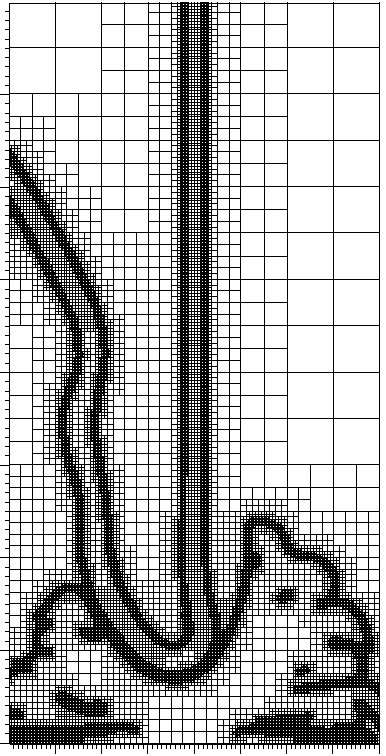
The experiments reported in Thrasher et al. [31], Binder and Landig [5], Lee et al. [25] suggest that a critical feature of bouncing jets is the occurrence of a thin layer between the jet and the rest of the fluid. These observations have led us to adopt a mesh refinement technique to describe accurately this thin layer. The refinement strategy is designed to increase the mesh resolution around the zero-level set of ΦΦ\Phi. More precisely, a cell K𝐾K is refined if its generation count (the number of times a cell from the initial subdivision has been refined to produce the current cell) is smaller than a given number Rmaxsubscript𝑅R_{\max} and if

|Φ(𝐱K,t)|βtanh(CR),Φsubscript𝐱𝐾𝑡𝛽subscript𝐶𝑅|\Phi({\bf x}_{K},t)|\leq\beta\tanh(C_{R}), (46)

where 𝐱Ksubscript𝐱𝐾{\bf x}_{K} is the barycenter of K𝐾K and CRsubscript𝐶𝑅C_{R} is an absolute constant. The purpose of the parameter Rmaxsubscript𝑅R_{\max} is to control the total number of cells. The parameter CRsubscript𝐶𝑅C_{R} controls the distance to the interface below which refinement occurs. Note that (46) is compatible with (38) and (42). The subdivisions are done with at most one hanging node per face, see e.g. Bonito and Nochetto [6, Section 6.3]. A cell is coarsen if it satisfies the following three conditions: its generation count is positive;

|Φ(𝐱K,t)|βtanh(CC),Φsubscript𝐱𝐾𝑡𝛽subscript𝐶𝐶|\Phi({\bf x}_{K},t)|\geq\beta\tanh(C_{C}), (47)

where CCCRsubscript𝐶𝐶subscript𝐶𝑅C_{C}\geq C_{R} is an absolute constant; and if once coarsened, the resulting subdivision does not have more than one hanging node per face. We refer to the documentation of the deal.II library for further details, Bangerth et al. [2].

4 Numerical Validations

The algorithm presented in the previous sections has been implemented using the deal.II finite element library described in Bangerth et al. [2, 3]. Parallelism is handled by using the MPI (Message Passing Interface) library, see Gabriel et al. [16]. The subdivision and mesh distribution is done by using the p4est library from Burstedde et al. [10].

The rest of this section illustrates and evaluates the performance of the above algorithm. We start in Section 4.1 by specifying all the numerical constants required by the algorithm. The validation of the transport code for solving the level-set equation in done Section 4.2. The validation of the two-phase fluid system is done in Section 4.3.

4.1 Numerical Parameters

Our algorithm involves several numerical parameters. In this section, we briefly recall their meaning, where they appear, and we specify the value of each of them. Unless specified otherwise these values are fixed for this entire section.

CCFLsubscript𝐶CFLC_{\text{CFL}} Cλsubscript𝐶𝜆C_{\lambda} CHsubscript𝐶𝐻C_{H} CSsubscript𝐶𝑆C_{S} CRsubscript𝐶𝑅C_{R} CCsubscript𝐶𝐶C_{C} Rmaxsubscript𝑅R_{\max} CLinsubscript𝐶LinC_{\text{Lin}} CEntsubscript𝐶EntC_{\text{Ent}} p𝑝p Cstabsubscript𝐶𝑠𝑡𝑎𝑏C_{stab}
Purpose CFL Reinitialization Adaptivity Stabilization
Appears in (27)&(36) (39) (42) (38) (46) (47) §3.5 (19) (18) (17) (33)
Value 0.25 0.01 1.25 0.5 2. 2. 2. 0.1 0.1 20 0.1
Table 1: Description and values of the numerical parameters.

A complete list of all the parameter is shown in Table 1. The parameter β𝛽\beta determining the width of the hyperbolic tangent filter (12) is defined to be β=minK𝒯hK𝛽subscript𝐾𝒯subscript𝐾\beta=\min_{K\in\mathcal{T}}h_{K}. This definition is used in the expression of the hyperbolic tangent filter (12), in the threshold of the approximate Heaviside function (42) and the approximate sign function (38), and in the refinement strategy (46)-(47).

4.2 Transport of the Level-Set

4.2.1 Convergence Tests

The consistency of the algorithm for the approximation of the level-set equation (3.1.3)-(24) is a priori third-order in time and space. To evaluate whether this is indeed the case, we solve the linear transport equation in the unit square Λ=(0,1)2Λsuperscript012\Lambda=(0,1)^{2} using the velocity field

𝐮(x,y,t):=(sin2(πx)sin(2πy)cos(πt/0.1)sin2(πy)sin(2πx)cos(πt/0.1)).assign𝐮𝑥𝑦𝑡superscript2𝜋𝑥2𝜋𝑦𝜋𝑡0.1superscript2𝜋𝑦2𝜋𝑥𝜋𝑡0.1{\bf u}(x,y,t):=\left(\begin{array}[]{r}-\sin^{2}(\pi x)\sin(2\pi y)\cos(\pi t/0.1)\\ \sin^{2}(\pi y)\sin(2\pi x)\cos(\pi t/0.1)\end{array}\right).

This flow is time-periodic of period 1, wich implies that ϕ(𝐱,0.2)=ϕ0(𝐱)italic-ϕ𝐱0.2subscriptitalic-ϕ0𝐱\phi({\bf x},0.2)=\phi_{0}({\bf x}), for all 𝐱Λ𝐱Λ{\bf x}\in\Lambda. The initial level-set function is chosen to be the signed distance to the line of equation y=0.5𝑦0.5y=0.5:

ϕ0(x,y)=y0.5.subscriptitalic-ϕ0𝑥𝑦𝑦0.5\phi_{0}(x,y)=y-0.5. (48)

The errors are evaluated at t=0.2𝑡0.2t=0.2. Three different scenarios are considered: (i) no stabilization and no reinitialization; (ii) entropy viscosity stabilization and no reinitialization; (iii) entropy viscosity and reinitialization, i.e., the complete algorithm. Except for β𝛽\beta, the values of the numerical parameters are given in Table 1. We consider four computations done on four uniform meshes with constant time steps. The mesh-size and the time step are divided by 222 each time. The meshes are composed of 1089, 4225, 16641and 66049 2subscript2{\mathbb{Q}}_{2} degree of freedoms. The space discretization is chosen fine enough not to influence the time error. We report in Table 2, the errors ΦNϕ0L2(Λ)subscriptnormsuperscriptΦ𝑁subscriptitalic-ϕ0superscript𝐿2Λ\|\Phi^{N}-\phi_{0}\|_{L^{2}(\Lambda)} for the three scenarios and the observed rates of convergence. Note that the reinitialization is turned on in scenario (iii), which implies that the exact solution at t=0.2𝑡0.2t=0.2 is not ϕ0subscriptitalic-ϕ0\phi_{0} anymore; we must instead compare ΦNsuperscriptΦ𝑁\Phi^{N} with βtanh(ϕ0(x,y)β)𝛽subscriptitalic-ϕ0𝑥𝑦𝛽\beta\tanh\left(\frac{\phi_{0}(x,y)}{\beta}\right). In this particular case we keep β𝛽\beta constant to ascertain the third-order consistency of the algorithm; we set β=0.0203125𝛽0.0203125\beta=0.0203125.

Scenario (i) Scenario (ii) Scenario (iii)
δt𝛿𝑡\delta t L2superscript𝐿2L^{2} error Observed rate L2superscript𝐿2L^{2} error Observed rate L2superscript𝐿2L^{2} error Observed rate
1e-2 1.2e-5 - 1.5e-5 - 1.3e-3 -
5e-3 1.5e-6 3. 1.8e-6 3. 1.5e-4 3.
2.5e-3 1.9e-7 3. 2.0e-7 3.2 2.0e-5 3.
1.25e-3 2.4e-8 3. 2.5e-8 3.1 2.6e-6 3.
Table 2: Single vortex test case: L2superscript𝐿2L^{2}-norm of error and observed convergence rates for each scenario after one period for different time discretization resolutions. (i) RK3 Galerkin algorithm; (ii) RK3 algorithm with entropy viscosity; (iii) RK3 with entropy viscosity and reinitialization. Third-order convergence rate is observed in all scenarios.

4.2.2 Rotation of a circular level-set: Effect of Different Viscosities and Reinitialization

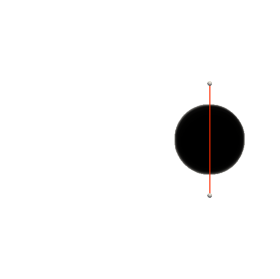
In this test case the initial data for the level set is the hyperbolic tangent filter applied to the distance to the circle centered at (0.5,0)0.50(0.5,0) and of radius 0.250.250.25

ϕ0(x,y):=βtanh(0.25((x0.5)2+y2)12β),(x,y)Λ:=(1,1)2,formulae-sequenceassignsubscriptitalic-ϕ0𝑥𝑦𝛽0.25superscriptsuperscript𝑥0.52superscript𝑦212𝛽𝑥𝑦Λassignsuperscript112\phi_{0}(x,y):=\beta\tanh\left(\frac{0.25-((x-0.5)^{2}+y^{2})^{\frac{1}{2}}}{\beta}\right),\qquad(x,y)\in\Lambda:=(-1,1)^{2},

see Figure 4(a). The level-set is transported by using the solid rotation velocity field:

𝐮(x,y):=(yx).assign𝐮𝑥𝑦𝑦𝑥{\bf u}(x,y):=\left(\begin{array}[]{r}-y\\ x\end{array}\right). (49)

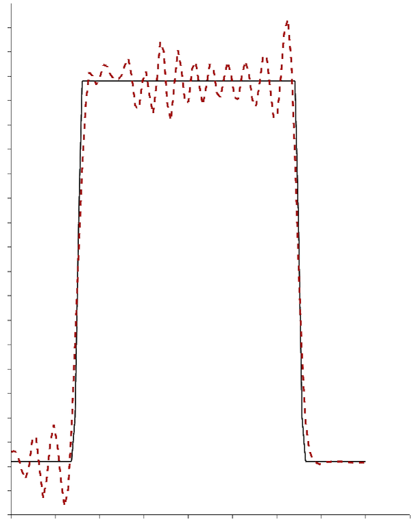
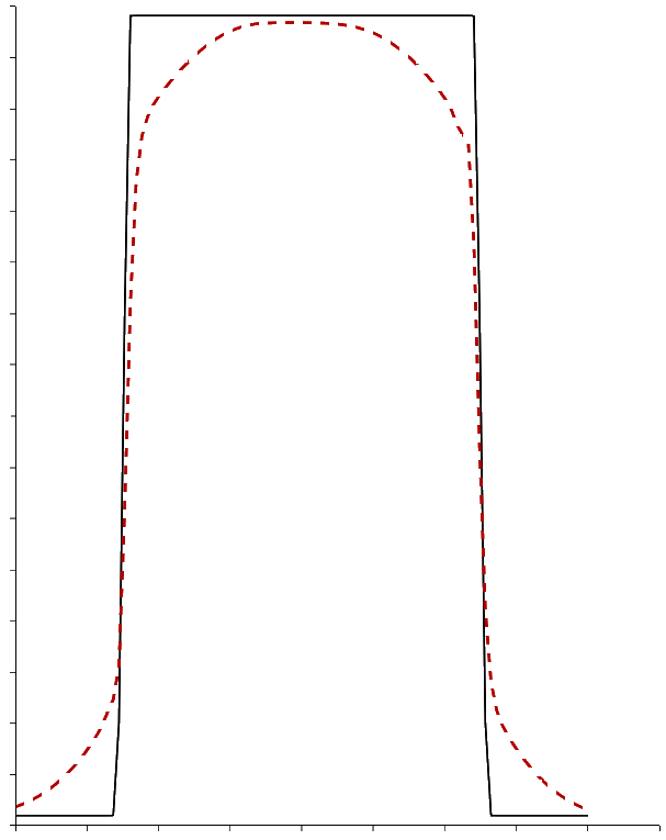
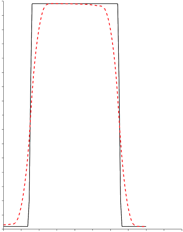
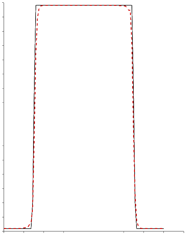
The computation is done with the adaptive algorithm described in Section 3.5 using Rmax=2subscript𝑅2R_{\max}=2. The initial mesh is uniform with hK=0.015625subscript𝐾0.015625h_{K}=0.015625 for all K𝒯𝐾𝒯K\in\mathcal{T}. The resulting time-dependent mesh is such that minT𝒯hK0.00390625subscript𝑇𝒯subscript𝐾0.00390625\min_{T\in\mathcal{T}}h_{K}\approx 0.00390625, i.e., we set β=0.00390625𝛽0.00390625\beta=0.00390625. The values of the other numerical constants are provided in Table 1. The time step δt𝛿𝑡\delta t is chosen to be uniform and equal to π×103𝜋superscript103\pi{\times}10^{-3}. We compare the initial level-set with its approximation after one revolution. Figures 4(b)-4(e) illustrate the benefits of using the entropy stabilization and the reinitialization technique by comparing the graphs of the exact and approximate level-set functions along the line of equation x=0.5𝑥0.5x=0.5 after one revolution.

Refer to caption
(a)
Refer to caption
(b)
Refer to caption
(c)
Refer to caption
(d)
Refer to caption
(e)
Figure 4: (a) Initial level-set: the dark region corresponds to ϕ00subscriptitalic-ϕ00\phi_{0}\geq 0; (b)-(e) Comparison of the graphs of the exact (solid line) and approximate (dashed line) level-set functions along the line of equation x=0.5𝑥0.5x=0.5 after one revolution: (b) without stabilization and reinitialization (CLin=CEnt=Cλ=0subscript𝐶Linsubscript𝐶Entsubscript𝐶𝜆0C_{\text{Lin}}=C_{\text{Ent}}=C_{\lambda}=0); (c) with first-order linear stabilization, CLin=0.1subscript𝐶Lin0.1C_{\text{Lin}}=0.1; (d) With entropy residual stabilization, CLin=0.1subscript𝐶Lin0.1C_{\text{Lin}}=0.1 and CEnt=0.1subscript𝐶Ent0.1C_{\text{Ent}}=0.1; (e) with entropy residual stabilization and reinitialization, Cλ=0.01subscript𝐶𝜆0.01C_{\lambda}=0.01. The transport without stabilization of the nearly discontinuous level-set function yields spurious oscillations. These oscillations are removed by the linear viscosity at the expense of large numerical diffusion. The numerical diffusion is minimized by turning on the entropy residual term. Finally, adding the reinitialization allows to nearly recover the exact profile.

4.2.3 3D Slotted Disk: Long Time Behavior

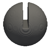
A typical benchmark for the transport of a level-set function is the so-called Zalesak disk documented in [36]. We consider in this section the three-dimensional version thereof. The computational domain is Λ:=(0,1)3assignΛsuperscript013\Lambda:=(0,1)^{3}. The initial level-set is the characteristic function of a slotted sphere centered at (0.5,0.75,0.5)0.50.750.5(0.5,0.75,0.5) with a radius of 0.150.150.15. The width, height and depth of the slot are 0.03750.03750.0375, 0.150.150.15, 0.30.30.3 respectively; see Figure 5(a)). The initial profile is transported by using the following velocity field:

𝐮(x,y,z):=(0.5yx0.50).assign𝐮𝑥𝑦𝑧0.5𝑦𝑥0.50{\bf u}(x,y,z):=\left(\begin{array}[]{r}0.5-y\\ x-0.5\\ 0\end{array}\right). (50)
Refer to caption
(a)
Refer to caption
(b)
Refer to caption
(c)
Refer to caption
(d)
Refer to caption
(e)
Refer to caption
(f)
Figure 5: Rotating Slotted three dimensional sphere. From left to right the dark regions corresponds to Φ0Φ0\Phi\geq 0 after 0,1,2,3,4 and 5 full rotations. Oscillations and numerical diffusion are controlled by the entropy viscosity as well as the reinitialization algorithm.

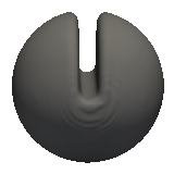
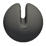
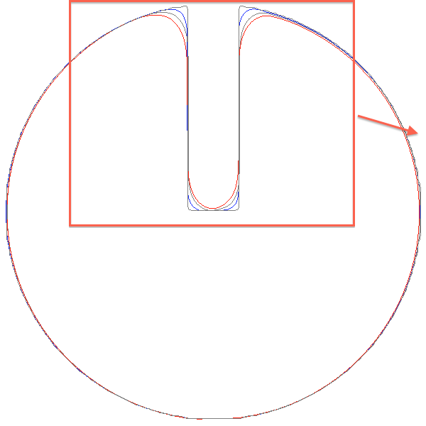
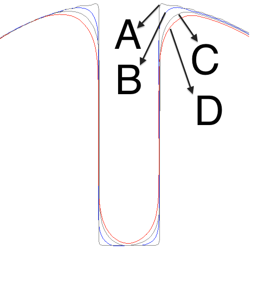
The time step is chosen to be uniform δt=π×103𝛿𝑡𝜋superscript103\delta t=\pi{\times}10^{-3}. The initial subdivision is composed of cells of diameter 0.0156250.0156250.015625. The adaptive mesh refinement technique described in Section 3.5 is used with Rmax=2subscript𝑅2R_{\max}=2; the minimum mesh size is minK𝒯hK=0.00390625subscript𝐾𝒯subscript𝐾0.00390625\min_{K\in\mathcal{T}}h_{K}=0.00390625. The numerical constants are given in Table 1. The computation is done until the slotted sphere has undergone 5 full revolutions. The iso-surface Φ=0Φ0\Phi=0 is shown in Figure 5 after each of the 5 periods. Oscillations and numerical diffusion are controlled by the entropy viscosity and the reinitialization algorithm. A closer look at the slotted region is provided in Figure 6.
Refer to caption
Refer to caption
Figure 6: Iso-contour Φ=0Φ0\Phi=0 in the plane z=0𝑧0z=0: (A) initial data; (B) after one rotation; (C) after three rotations; (D) after five rotations. Numerical diffusion is observed but is greatly minimized by the entropy viscosity and reinitialization techniques.

4.2.4 Single Vortex: Large Deformations

The Single Vortex problem consists of the deformation of a sphere by a time-periodic incompressible vortex-like flow. The computational domain is Λ=(0,1)3Λsuperscript013\Lambda=(0,1)^{3}, and the time-periodic velocity field is defined by

𝐮(x,y,t):=(sin2(πx)sin(2πy)cos(πt/4)sin2(πy)sin(2πx)cos(πt/4)0).assign𝐮𝑥𝑦𝑡superscript2𝜋𝑥2𝜋𝑦𝜋𝑡4superscript2𝜋𝑦2𝜋𝑥𝜋𝑡40{\bf u}(x,y,t):=\left(\begin{array}[]{c}-\sin^{2}(\pi x)\sin(2\pi y)\cos(\pi t/4)\\ \sin^{2}(\pi y)\sin(2\pi x)\cos(\pi t/4)\\ 0\end{array}\right). (51)

The initial level-set is given by

ϕ0(𝐱):=βtanh(dist(S,𝐱)β),assignsubscriptitalic-ϕ0𝐱𝛽dist𝑆𝐱𝛽\phi_{0}({\bf x}):=\beta\tanh\left(\frac{\mbox{dist}(S,{\bf x})}{\beta}\right), (52)

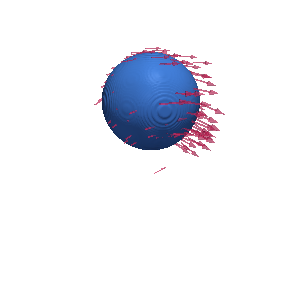
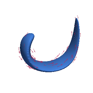
where S𝑆S is the sphere centered at (0.5,0.75,0.5)0.50.750.5(0.5,0.75,0.5) of radius of 0.150.150.15. The field ϕ0subscriptitalic-ϕ0\phi_{0} is a regularized version of the distance function using the tanh\tanh cut-off filter (12). The divergence-free velocity field severely deforms the level-set until t=2𝑡2t=2 and returns it to its initial shape at t=4𝑡4t=4. The time step is chosen to be uniform δt=0.001𝛿𝑡0.001\delta t=0.001 and the final time is t=4𝑡4t=4 (1 cycle). The initial subdivision is made of uniform cells of diameter 0.0156250.0156250.015625; the minimum mesh size allowed in the adaptive mesh refinement is 0.003906250.003906250.00390625. The numerical constants are given in Table 1. Figure 7 shows the iso-contour Φ=0Φ0\Phi=0 at different times. The undeformed sphere is recovered after one cycle.
Refer to caption
Refer to caption
Refer to caption
Refer to caption
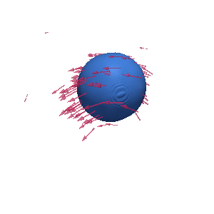
Figure 7: 3D Vortex using (51). From left to right: t=0𝑡0t=0, t=1𝑡1t=1, t=3𝑡3t=3, t=4𝑡4t=4. The initial sphere is recovered after one cycle. The vectors indicate the direction of the velocity field.
4.3 Two Phase Flows

4.3.1 Rising Bubble: Surface Tension Benchmark

We start the validation of the two phase flow system with the Rising bubble benchmark problem, wee e.g. Hysing et al. [23]. The computational domain is Λ=(0,1)×(0,2)Λ0102\Lambda=(0,1){\times}(0,2), the initial data ϕ0subscriptitalic-ϕ0\phi_{0} is the characteristic function of a circular bubble of radius 0.250.250.25 centered at (0.5,0.5)0.50.5(0.5,0.5). Two different sets of physical constants are considered, see Table 3; σ𝜎\sigma is the surface tension coefficient and g𝑔g is the magnitude of the non-dimensional gravitational force. The domains Ω+superscriptΩ\Omega^{+} and ΩsuperscriptΩ\Omega^{-} are the domains inside and outside the bubble, respectively. The no-slip boundary condition is imposed at the top and bottom of the computational domain. The free slip condition (2c) is imposed on the side walls.

Test case ρ+superscript𝜌\rho^{+} ρsuperscript𝜌\rho^{-} μ+superscript𝜇\mu^{+} μsuperscript𝜇\mu^{-} g𝑔g σ𝜎\sigma
1 1000 100 10 1. 0.98 24.5
2 1000 1 10 0.1 0.98 1.96
Table 3: Two different sets of physical constants for the rising bubble benchmark problems. The first test case consists of a density/viscosity ratio of 10 with a large surface tension coefficient. The density/viscosity ratio is equal to 100 in the second case and the surface tension coefficient is smaller.

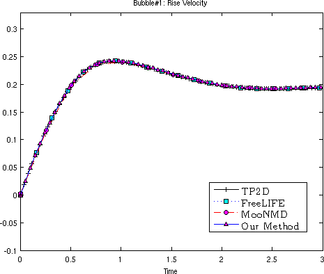
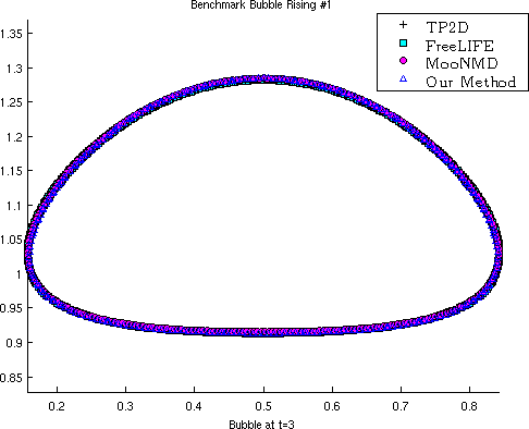
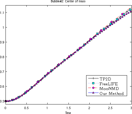
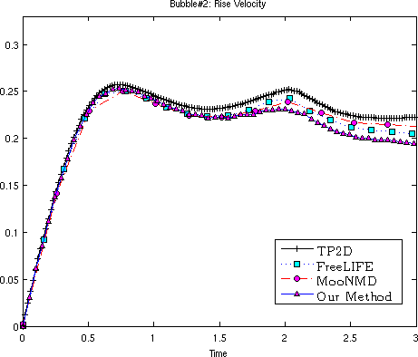
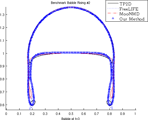
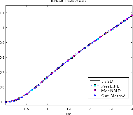
The initial subdivision is made of uniform cells of diameter 0.031250.031250.03125; the minimum mesh size allowed in the adaptive mesh refinement is 0.00781250.00781250.0078125. The time steps δt𝛿𝑡\delta t are chosen uniform according to the CFL restriction (27) and the values of the numerical constants are given in Table 1. We compare in Figure 8 our results with those from three other methods. We show in panel (a) the time history of the center of mass 𝐗c:=Ω2𝐱𝑑𝐱/Ω21𝑑𝐱assignsubscript𝐗𝑐subscriptsubscriptΩ2𝐱differential-d𝐱subscriptsubscriptΩ21differential-d𝐱{\bf X}_{c}:=\int_{\Omega_{2}}{\bf x}d{\bf x}/\int_{\Omega_{2}}1d{\bf x}, in panel (b) the rising velocity uc:=Ω2uy𝑑𝐱/Ω21𝑑𝐱assignsubscript𝑢𝑐subscriptsubscriptΩ2subscript𝑢𝑦differential-d𝐱subscriptsubscriptΩ21differential-d𝐱u_{c}:=\int_{\Omega_{2}}u_{y}d{\bf x}/\int_{\Omega_{2}}1d{\bf x}, and in panel (c) the shape of the bubble at t=3𝑡3t=3. The results of our simulations are within the range of those given by the benchmark algorithms.
Refer to caption
(a) Center of Mass, case #1#1\#1
Refer to caption
(b) Rise Velocity, case #1#1\#1
Refer to caption
(c) Zero level-set at t=3𝑡3t=3, case #1#1\#1
Refer to caption
(d) Center of Mass, case #2#2\#2
Refer to caption
(e) Rise Velocity, case #2#2\#2
Refer to caption
(f) Zero level-set at t=3𝑡3t=3, case #2#2\#2
Figure 8: Rising bubble test cases #1#1\#1 and #2#2\#2. Our simulations are within the range of the benchmark.

The shape of the bubble for the test case #2 at t=3𝑡3t=3 is reported in Figure 9 and compared with the shapes obtained by the other algorithms described in Hysing et al. [23].

Refer to caption
Figure 9: Rising bubble case #2#2\#2 at t=3𝑡3t=3. Different algorithms described in Hysing et al. [23] and our simulation in the rightmost panel. The shapes of the bubbles are qualitatively similar. The left figures are courtesy of S. Turek bub [1].

4.3.2 Buckling fluids

We now test the algorithm in the context of fluid buckling, see for instance Ville et al. [35], Tome and McKee [32], Bonito et al. [7]. The test consists of letting a free-falling jet of very viscous fluid impinge on a horizontal surface. The diameter of the impinging jet is 0.1 mtimes0.1meter0.1\text{\,}\mathrm{m} and the inflow velocity is 1 m s1times1timesmetersecond11\text{\,}\mathrm{m}\text{\,}{\mathrm{s}}^{-1} in Λ=(0,1 m)2Λsuperscript0times1meter2\Lambda=(0,$1\text{\,}\mathrm{m}$)^{2}. The physical parameters chosen for the falling fluid are ρ+=1800 kg m3superscript𝜌times1800timeskilogrammeter3\rho^{+}=$1800\text{\,}\mathrm{kg}\text{\,}{\mathrm{m}}^{-3}$, μ+=250 Pa ssuperscript𝜇times250timespascalsecond\mu^{+}=$250\text{\,}\mathrm{Pa}\text{\,}\mathrm{s}$ and ρ=1 kg m3superscript𝜌times1timeskilogrammeter3\rho^{-}=$1\text{\,}\mathrm{kg}\text{\,}{\mathrm{m}}^{-3}$, μ=2×10⁵ Pa ssuperscript𝜇times2E-5timespascalsecond\mu^{-}=$2\text{\times}{10}^{-5}\text{\,}\mathrm{Pa}\text{\,}\mathrm{s}$ for the ambient fluid as in Ville et al. [35]. The no-slip boundary condition (𝐮=𝟎𝐮0{\bf u}=\bf{0}) is imposed at the bottom boundary, and an inflow boundary condition is imposed where |x0.5|<0.05𝑥0.50.05|x-0.5|<0.05 at the top boundary. The open boundary condition is enforced on all the other boundaries, i.e., (2μS𝐮pI)𝝂=02𝜇superscript𝑆𝐮𝑝𝐼𝝂0(2\mu\nabla^{S}{\bf u}-pI){\boldsymbol{\nu}}=0. Surface tension is neglected for this test case (σ=0𝜎0\sigma=0). The numerical constants are given in Table 1.

The initial subdivision is composed of cells of uniform diameter 0.015 625 mtimes0.015625meter0.015\,625\text{\,}\mathrm{m}, and the minimum cell diameter reached during the mesh adaption process is 0.003 906 mtimes0.003906meter0.003\,906\text{\,}\mathrm{m}. The time evolution of the fluid is shown in Figure 10. Buckling occurs after the viscous fluid impacts the rigid bottom plate.

Refer to caption
Refer to caption
Refer to caption
Refer to caption
Refer to caption
Figure 10: (From left to right) Time evolution of a jet of very viscous liquid inside a cavity filled with air. Buckling occurs when the liquid hits the floor.
Refer to caption Refer to caption Refer to caption Refer to caption Refer to caption Refer to caption
(a) (b) (c) (d) (e) (f)
Figure 11: (a)-(e) Time evolution of a three-dimensional jet of Silicone oil falling in a cavity filled with air at time (a) t=0.00501s𝑡0.00501𝑠t=0.00501~{}s, (b) t=0.0209s𝑡0.0209𝑠t=0.0209~{}s, (c) t=0.031s𝑡0.031𝑠t=0.031~{}s, (d) t=0.04099s𝑡0.04099𝑠t=0.04099~{}s, and (e) t=0.048998s𝑡0.048998𝑠t=0.048998~{}s. For comparison, (f) shows the shape of the Silicone oil jet obtained in laboratory with the same physical conditions. Our numerical simulations are qualitatively in agreement with the physical experiment.

We also show in Figure 11 a three-dimensional simulation. The computational domain is Λ=(0,0.008 m)3Λsuperscript0times0.008meter3\Lambda=(0,$0.008\text{\,}\mathrm{m}$)^{3}, the initial diameter of the jet is 0.0004 mtimes0.0004meter0.0004\text{\,}\mathrm{m} and the inflow velocity is 1.75 m s1times1.75timesmetersecond11.75\text{\,}\mathrm{m}\text{\,}{\mathrm{s}}^{-1}. The viscosity and density of the fluid are those of silicone oil: ρ+=960 kg m3superscript𝜌times960timeskilogrammeter3\rho^{+}=$960\text{\,}\mathrm{kg}\text{\,}{\mathrm{m}}^{-3}$, μ+=5 Pa ssuperscript𝜇times5timespascalsecond\mu^{+}=$5\text{\,}\mathrm{Pa}\text{\,}\mathrm{s}$. The viscosity and density of the ambient fluid are those of air: ρ=1.2 kg m3superscript𝜌times1.2timeskilogrammeter3\rho^{-}=$1.2\text{\,}\mathrm{kg}\text{\,}{\mathrm{m}}^{-3}$, μ=2×10⁵ Pa ssuperscript𝜇times2E-5timespascalsecond\mu^{-}=$2\text{\times}{10}^{-5}\text{\,}\mathrm{Pa}\text{\,}\mathrm{s}$. Surface tension is accounted for, σ=0.021 N m1𝜎times0.021timesnewtonmeter1\sigma=$0.021\text{\,}\mathrm{N}\text{\,}{\mathrm{m}}^{-1}$. The no-slip boundary condition (𝐮=𝟎𝐮0{\bf u}=\bf{0}) is imposed at the bottom of the box. The inflow boundary is the disk (x0.004)2+(y0.004)2<0.0002superscript𝑥0.0042superscript𝑦0.00420.0002\sqrt{(x-0.004)^{2}+(y-0.004)^{2}}<0.0002 at the top boundary (z=0.008𝑧0.008z=0.008). Open boundary conditions (2μS𝐮pI)𝝂=02𝜇superscript𝑆𝐮𝑝𝐼𝝂0(2\mu\nabla^{S}{\bf u}-pI){\boldsymbol{\nu}}=0 are applied on the rest of the boundary. The results are obtained with adaptive mesh refinement with the minimum cell diameter 6.25×10⁵ mtimes6.25E-5meter6.25\text{\times}{10}^{-5}\text{\,}\mathrm{m}. The time steps follow the CFL restriction (27) and the numerical constants are given in Table 1.

5 Numerical Simulations of Bouncing Jets

We now use our algorithm to predict the bouncing effect of jets of Newtonian (Section 5.1) and non-Newtonian (Section 5.2)fluids. In both cases, the formation of a thin layer of air between the jet and the bulk of the fluid is a critical ingredient to observe the bouncing effect. The adaptive mesh refinement strategy adopted in our algorithm allows to capture this thin layer with a reasonable number of degrees of freedom.

5.1 Two-dimensional Newtonian Bouncing Jets

We start with a Newtonian fluid falling into a translating bath as in the experiment proposed in Thrasher et al. [31]. The fluid is a silicone oil with viscosity μ+=0.25 Pa ssuperscript𝜇times0.25timespascalsecond\mu^{+}=$0.25\text{\,}\mathrm{Pa}\text{\,}\mathrm{s}$ and density ρ+=960 kg m3superscript𝜌times960timeskilogrammeter3\rho^{+}=$960\text{\,}\mathrm{kg}\text{\,}{\mathrm{m}}^{-3}$. The ambient fluid is air: ρ=1.2 kg m3superscript𝜌times1.2timeskilogrammeter3\rho^{-}=$1.2\text{\,}\mathrm{kg}\text{\,}{\mathrm{m}}^{-3}$ and μ=2×10⁵ Pa ssuperscript𝜇times2E-5timespascalsecond\mu^{-}=$2\text{\times}{10}^{-5}\text{\,}\mathrm{Pa}\text{\,}\mathrm{s}$. The computational domain is Λ:=(0,0.04 cm)×(0,0.06 cm)assignΛ0times0.04centimeter0times0.06centimeter\Lambda:=(0,$0.04\text{\,}\mathrm{cm}$){\times}(0,$0.06\text{\,}\mathrm{cm}$). The radius of the incoming jet is 0.25 cmtimes0.25centimeter0.25\text{\,}\mathrm{cm}; its velocity is 𝐮=(0,5 cm s1)𝐮0times5timescentimetersecond1{\bf u}=(0,-$5\text{\,}\mathrm{cm}\text{\,}{\mathrm{s}}^{-1}$) on {(x,y)Λ:y=4,|x0.01|<0.0025}conditional-set𝑥𝑦Λformulae-sequence𝑦4𝑥0.010.0025\{(x,y)\in\partial\Lambda\ :y=4,\ |x-0.01|<0.0025\}. The region {(x,y)Λ: 0<y<0.02}conditional-set𝑥𝑦Λ 0𝑦0.02\{(x,y)\in\Lambda\ :\ 0<y<0.02\} is filled by the same fluid, called the “bath”, and it moves to the right with a horizontal velocity VBsubscript𝑉𝐵V_{B} to be specified later. Slip boundary condition (2c) are imposed at the bottom of the cavity and the open boundary condition (2μS𝐮pI)𝝂=02𝜇superscript𝑆𝐮𝑝𝐼𝝂0(2\mu\nabla^{S}{\bf u}-pI){\boldsymbol{\nu}}=0 is applied to the rest of the boundary

{(x,y)Λ:y=4,|x0.01|0.0025}{(x,y)Λ:x=0,y0.02}{(x,y)Λ:x=0.04}.conditional-set𝑥𝑦Λformulae-sequence𝑦4𝑥0.010.0025conditional-set𝑥𝑦Λformulae-sequence𝑥0𝑦0.02conditional-set𝑥𝑦Λ𝑥0.04\{(x,y)\in\partial\Lambda\ :\ y=4,\ |x-0.01|\geq 0.0025\}\cup\{(x,y)\in\partial\Lambda\ :\ x=0,\ y\geq 0.02\}\cup\{(x,y)\in\partial\Lambda\ :\ x=0.04\}.

The values of the numerical constants are those given in Table 1. The minimum cell diameter resulting from the adaptive mesh refinement strategy is 7.8125×10⁵ cmtimes7.8125E-5centimeter7.8125\text{\times}{10}^{-5}\text{\,}\mathrm{cm}. The time steps are chosen to satisfy the CFL restriction (27).

As already noted in Thrasher et al. [31], there is a range of velocities for which bouncing occurs, but the jet slides along the surface of the bath when the horizontal velocity of the bath is too high. This is illustrated in Figures 12(a) and 12(b): the jet bounces when VB=8 cm s1subscript𝑉𝐵times8timescentimetersecond1V_{B}=$8\text{\,}\mathrm{cm}\text{\,}{\mathrm{s}}^{-1}$ (see Figure 12(a)) but it slides when VB=25 cm s1subscript𝑉𝐵times25timescentimetersecond1V_{B}=$25\text{\,}\mathrm{cm}\text{\,}{\mathrm{s}}^{-1}$ (see Figure 12(b)). Note that it is necessary to include the surface tension to keep the jet stable after impinging on the free surface as illustrated in Figure 12(c) where a simulation without surface tension is presented. Observe finally that all our numerical simulations show that a thin layer of air is formed between the jet and the bath each time the jet bounces.

Refer to caption
Refer to caption
Refer to caption
Refer to caption
(a)
Refer to caption
Refer to caption
Refer to caption
Refer to caption
(b)
Refer to caption
Refer to caption
Refer to caption
Refer to caption
(c)
Figure 12: Newtonian bouncing jet (from left to right). The white arrow indicates the translation direction of the bath. (a) Bath velocity VB=8 cm s1subscript𝑉𝐵times8timescentimetersecond1V_{B}=$8\text{\,}\mathrm{cm}\text{\,}{\mathrm{s}}^{-1}$ and surface tension coefficient σ=21 mN m1𝜎times21timesmillinewtonmeter1\sigma=$21\text{\,}\mathrm{mN}\text{\,}{\mathrm{m}}^{-1}$; the incoming jet bounces away from the bath and we observe the apparition of an air layer between the jet and the bath. (b) Bath velocity VB=25 cm s1subscript𝑉𝐵times25timescentimetersecond1V_{B}=$25\text{\,}\mathrm{cm}\text{\,}{\mathrm{s}}^{-1}$ and surface tension coefficient σ=21 mN m1𝜎times21timesmillinewtonmeter1\sigma=$21\text{\,}\mathrm{mN}\text{\,}{\mathrm{m}}^{-1}$; in this case, the bath velocity is too large and the jet slides along the bath surface; (c) Bath velocity VB=8 cm s1subscript𝑉𝐵times8timescentimetersecond1V_{B}=$8\text{\,}\mathrm{cm}\text{\,}{\mathrm{s}}^{-1}$ but without surface tension σ=0 mN m1𝜎times0timesmillinewtonmeter1\sigma=$0\text{\,}\mathrm{mN}\text{\,}{\mathrm{m}}^{-1}$; compare with (a).

5.2 Kaye Effect

The Kaye effect is the name given to the bouncing jet phenomenon when the bath is stationary. This effect has been observed to occur only with non-Newtonian fluids. It is now recognized that shear-thinning viscosity is a critical component of the Kaye effects, see e.g. Collyer and Fischer [12], Versluis et al. [34], Binder and Landig [5]. Following Versluis et al. [34], we adopt the model of Cross [13] in the rest of the paper

μ(γ)=μ+μ0μ1+(γγc)n,𝜇𝛾subscript𝜇subscript𝜇0subscript𝜇1superscript𝛾subscript𝛾𝑐𝑛\mu(\gamma)=\mu_{\infty}+\dfrac{\mu_{0}-\mu_{\infty}}{1+\left(\dfrac{\gamma}{\gamma_{c}}\right)^{n}}, (53)

where μ0subscript𝜇0\mu_{0} is the viscosity at zero shear stress, μsubscript𝜇\mu_{\infty} is the limiting viscosity for large stresses, γ𝛾\gamma is the Frobenius norm of the rate-of-strain tensor

γ:=S𝐮:=(i=1dj=1d14(𝐮j𝐱i+𝐮i𝐱j)2)12assign𝛾normsuperscript𝑆𝐮assignsuperscriptsuperscriptsubscript𝑖1𝑑superscriptsubscript𝑗1𝑑14superscriptsubscript𝐮𝑗subscript𝐱𝑖subscript𝐮𝑖subscript𝐱𝑗212\gamma:=\|\nabla^{S}{\bf u}\|:=\left(\sum_{i=1}^{d}\sum_{j=1}^{d}\frac{1}{4}\left(\frac{\partial{\bf u}_{j}}{\partial{\bf x}_{i}}+\frac{\partial{\bf u}_{i}}{\partial{\bf x}_{j}}\right)^{2}\right)^{\frac{1}{2}}

and γcsubscript𝛾𝑐\gamma_{c}, n𝑛n are two additional parameters. As a benchmark, we consider a commercial shampoo for which the shear-thinning constants corresponding to the above model (53) have been identified experimentally in Lee et al. [25]. Recall that viscosities cannot be measured directly but are deduced from velocity and displacement measurements so as to match in some least-squares sense a behavior conjectured a-priori. The parameters μ0subscript𝜇0\mu_{0}, μsubscript𝜇\mu_{\infty}, γcsubscript𝛾𝑐\gamma_{c}, n𝑛n corresponding to the model (53) obtained in Lee et al. [25] are

μ0=5.7 Pa s,μ=103 Pa s,γc=15 s1,andn=1.formulae-sequencesubscript𝜇0times5.7timespascalsecondformulae-sequencesubscript𝜇timesE-3timespascalsecondformulae-sequencesubscript𝛾𝑐times15second1and𝑛1\mu_{0}=$5.7\text{\,}\mathrm{Pa}\text{\,}\mathrm{s}$,\quad\mu_{\infty}=${10}^{-3}\text{\,}\mathrm{Pa}\text{\,}\mathrm{s}$,\quad\gamma_{c}=$15\text{\,}{\mathrm{s}}^{-1}$,\quad\mathrm{and}\quad n=1. (54)

We show in Figure 13 snapshots of experiments done with the shampoo poured at different flow rate. It was observed unambiguously in Lee et al. [25] that the jet slides on a lubricating air layer.
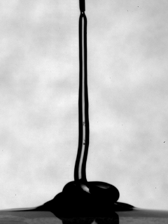
Refer to caption
(a) 5 ml/min
Refer to caption
(b) 6 ml/min
Refer to caption
(c) 7 ml/min
Refer to caption
(d) 8 ml/min
Figure 13: Shampoo poured at different flow rates (a) 5 mL min1times5timesmilliliterminute15\text{\,}\mathrm{mL}\text{\,}{\mathrm{min}}^{-1}; (b) 6 mL min1times6timesmilliliterminute16\text{\,}\mathrm{mL}\text{\,}{\mathrm{min}}^{-1}; (c) 7 mL min1times7timesmilliliterminute17\text{\,}\mathrm{mL}\text{\,}{\mathrm{min}}^{-1}; and (d) 8 mL min1times8timesmilliliterminute18\text{\,}\mathrm{mL}\text{\,}{\mathrm{min}}^{-1}; No bouncing is observed at low flow rate (a) and (b). However, the Kaye effect is observed at higher flow rate (c) and (d).

In order to reproduce qualitatively the above experiments we consider the two-dimensional computational domain Λ=(0.496 m,0.594 m)×(0,0.016 m)Λtimes0.496metertimes0.594meter0times0.016meter\Lambda=($0.496\text{\,}\mathrm{m}$,$0.594\text{\,}\mathrm{m}$){\times}(0,$0.016\text{\,}\mathrm{m}$). The no-slip boundary condition (𝐮=𝟎𝐮0{\bf u}=\bf{0}) is imposed at the bottom of the computational domain and an inflow boundary condition is imposed on the disk {(x,y)||x0.5|<0.00021875}conditional-set𝑥𝑦𝑥0.50.00021875\{(x,y)\ |\ |x-0.5|<0.00021875\} on the top of the box. This correspond to a jet of radius 0.4375 mmtimes0.4375millimeter0.4375\text{\,}\mathrm{mm}. The inflow velocity is taken to be 1.75 m s1times1.75timesmetersecond11.75\text{\,}\mathrm{m}\text{\,}{\mathrm{s}}^{-1}. The open boundary condition (2μS𝐮pI)𝝂=02𝜇superscript𝑆𝐮𝑝𝐼𝝂0(2\mu\nabla^{S}{\bf u}-pI){\boldsymbol{\nu}}=0 is applied on all the other boundaries. The numerical constants used in the simulations are listed in Table 1. The minimum mesh size attainable by adaptive mesh refinement is 3.125×10⁵ mtimes3.125E-5meter3.125\text{\times}{10}^{-5}\text{\,}\mathrm{m}, and time steps are chosen to comply with the CFL restriction (27). The physical parameters chosen for the fluid are ρ+=1020 kg m3superscript𝜌times1020timeskilogrammeter3\rho^{+}=$1020\text{\,}\mathrm{kg}\text{\,}{\mathrm{m}}^{-3}$, the shear-thinning viscosity constants are provided in (55). We take ρ=1.2 kg m3superscript𝜌times1.2timeskilogrammeter3\rho^{-}=$1.2\text{\,}\mathrm{kg}\text{\,}{\mathrm{m}}^{-3}$ and μ=2×10⁵ Pa ssuperscript𝜇times2E-5timespascalsecond\mu^{-}=$2\text{\times}{10}^{-5}\text{\,}\mathrm{Pa}\text{\,}\mathrm{s}$ for the air. Surface tension is applied at the fluid/air interface with the surface tension coefficient σ=0.03 N m1𝜎times0.03timesnewtonmeter1\sigma=$0.03\text{\,}\mathrm{N}\text{\,}{\mathrm{m}}^{-1}$.

After many numerical experiments it turned out that the above physical parameters did not give any Kaye effect. Our interpretation is that the shear-thinning effect given by the set of parameters (54) is too strong; with these coefficients the fluid instantly becomes water-like when hitting the bottom of the cavity, see Figure 14(a). Several explanations for this mismatch are plausible: (i) as mentioned above the parameters (54) are measured under the assumption that the shear-thinning law follows the Cross model; (ii) the shear is over-predicted by our algorithm; (iii) the air layer width for this range of parameters is too thin to be captured by the algorithm; (iv) a fundamental component is missing in our mathematical model. These observations have lead us to consider a different set of shear-thinning parameters requiring a larger shear for a notable reduction of the viscosity and a smoother transition from the maximum to the minimum values of the viscosity, see Figure 14(b). The parameters that we now consider are the following:

μ0=5.7 Pa s,μ=103 Pa s,γc=970 s1andn=3.formulae-sequencesubscript𝜇0times5.7timespascalsecondformulae-sequencesubscript𝜇timesE-3timespascalsecondformulae-sequencesubscript𝛾𝑐times970second1and𝑛3\mu_{0}=$5.7\text{\,}\mathrm{Pa}\text{\,}\mathrm{s}$,\quad\mu_{\infty}=${10}^{-3}\text{\,}\mathrm{Pa}\text{\,}\mathrm{s}$,\quad\gamma_{c}=$970\text{\,}{\mathrm{s}}^{-1}$\quad\mathrm{and}\quad n=3. (55)
Refer to caption
(a) Jet with parameters (54)
Refer to caption
(b) Redefined viscosity
Figure 14: (Left) Falling jet of liquid described by the parameters given in (54). The shear-thinning effect is too strong and the fluid becomes instantly water-like when hitting the bottom of the cavity. (Right) Viscosity vs Shear for the parameters (54) (dotted line) and (55) (solid line).

This set of parameter produces the Kaye effect as shown in Figure 15. Here again we notice that there is a very thin layer of air between the bouncing jet and the rest of the fluid, thereby adding to the large body of evidence pointing at the importance of air layers in bouncing jets. Let us finally mention that these computations show also that mesh adaptivity is critical to reproduce numerically the Kaye effect.
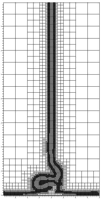
Refer to caption
Refer to caption
Refer to caption
Refer to caption
Refer to caption
Refer to caption
Refer to caption
Refer to caption
Refer to caption
Refer to caption
Refer to caption
Refer to caption
Figure 15: (Left to Right, Top to Bottom) Numerical simulation of the Kaye effect with adaptive meshes (from left to right and top to bottom). The viscosity parameters are given in (55). The first and last frames illustrate the adaptive subdivision generated by the adaptive strategy. An air layer appears in the last frame in the first row and is fully developed in the first frame of the second row. The apparition of the air layer coincides with the beginning of the bouncing phenomenon.

Acknowledgments

The experiments reported in the paper were done at the High Speed Fluid Imaging Laboratory of S. Thoroddsen at KAUST during two visits of S.L. The authors would like to express their gratitude to S. Thoroddsen and E. Li for their help in conducting these experiments. W. Bangerth availability and his constant help in the implementation of our algorithms with the deal.II library is acknowledged. The authors acknowledge the Texas A&M University Brazos HPC cluster that contributed to the research reported here.

References

  • bub [2014] Rising bubble benchmark problems, 2014. URL http://www.featflow.de/en/benchmarks/cfdbenchmarking/bubble.html.
  • Bangerth et al. [2007] W. Bangerth, R. Hartmann, and G. Kanschat. deal.II — a general purpose object oriented finite element library. ACM Trans. Math. Softw., 33(4), 2007.
  • Bangerth et al. [2013] W. Bangerth, T. Heister, L. Heltai, G. Kanschat, M. Kronbichler, M. Maier, B. Turcksin, and T. D. Young. The deal.ii library, version 8.1. arXiv preprint, 2013.
  • Bänsch [2001] E. Bänsch. Finite element discretization of the Navier-Stokes equations with a free capillary surface. Numer. Math., 88(2):203–235, 2001. ISSN 0029-599X.
  • Binder and Landig [2009] J. M. Binder and A. J. Landig. The kaye effect. European Journal of Physics, 30(6):S115, 2009.
  • Bonito and Nochetto [2010] A. Bonito and R. H. Nochetto. Quasi-optimal convergence rate of an adaptive discontinuous Galerkin method. SIAM J. Numer. Anal., 48(2):734–771, 2010. ISSN 0036-1429.
  • Bonito et al. [2006] A. Bonito, M. Picasso, and M. Laso. Numerical simulation of 3D viscoelastic flows with free surfaces. J. Comput. Phys., 215(2):691–716, 2006. ISSN 0021-9991.
  • Bonito et al. [2014] A. Bonito, J.-L. Guermond, and B. Popov. Stability analysis of explicit entropy viscosity methods for non-linear scalar conservation equations. Math. Comp., 83(287):1039–1062, 2014. ISSN 0025-5718.
  • Bonito et al. [to appear] A. Bonito, J.-L. Guermond, and S. Lee. Modi ed pressure-correction projection methods: Open boundary and variable time stepping. In Proceedings of the 10th European Conference (ENUMATH 2013), to appear.
  • Burstedde et al. [2011] C. Burstedde, L. C. Wilcox, and O. Ghattas. p4est: Scalable algorithms for parallel adaptive mesh refinement on forests of octrees. SIAM Journal on Scientific Computing, 33(3):1103–1133, 2011.
  • Chorin [1968] A. J. Chorin. Numerical solution of the Navier-Stokes equations. Math. Comp., 22:745–762, 1968. ISSN 0025-5718.
  • Collyer and Fischer [1976] A. Collyer and P. J. Fischer. The kaye effect revisited. Nature, 261:682, 1976.
  • Cross [1965] M. M. Cross. Rheology of non-newtonian fluids: A new flow equation for pseudoplastic systems. Journal of Colloid Science, 20(5):417 – 437, 1965.
  • Dziuk and Elliott [2010] G. Dziuk and C. M. Elliott. An Eulerian approach to transport and diffusion on evolving implicit surfaces. Comput. Vis. Sci., 13(1):17–28, 2010. ISSN 1432-9360.
  • Engquist et al. [2005] B. Engquist, A.-K. Tornberg, and R. Tsai. Discretization of Dirac delta functions in level set methods. J. Comput. Phys., 207(1):28–51, 2005. ISSN 0021-9991.
  • Gabriel et al. [2004] E. Gabriel, G. E. Fagg, G. Bosilca, T. Angskun, J. J. Dongarra, J. M. Squyres, V. Sahay, P. Kambadur, B. Barrett, A. Lumsdaine, R. H. Castain, D. J. Daniel, R. L. Graham, and T. S. Woodall. Open MPI: Goals, concept, and design of a next generation MPI implementation. In Proceedings, 11th European PVM/MPI Users’ Group Meeting, pages 97–104, Budapest, Hungary, September 2004.
  • Gilbarg and Trudinger [2001] D. Gilbarg and N. S. Trudinger. Elliptic partial differential equations of second order. Classics in Mathematics. Springer-Verlag, Berlin, 2001. ISBN 3-540-41160-7. Reprint of the 1998 edition.
  • Gottlieb et al. [2001] S. Gottlieb, C.-W. Shu, and E. Tadmor. Strong stability-preserving high-order time discretization methods. SIAM review, 43(1):89–112, 2001.
  • Guermond and Salgado [2009] J.-L. Guermond and A. Salgado. A splitting method for incompressible flows with variable density based on a pressure poisson equation. Journal of Computational Physics, 228(8):2834 – 2846, 2009. ISSN 0021-9991.
  • Guermond and Shen [2004] J. L. Guermond and J. Shen. On the error estimates for the rotational pressure-correction projection methods. Math. Comp., 73(248):1719–1737 (electronic), 2004. ISSN 0025-5718.
  • Guermond et al. [2005] J. L. Guermond, P. Minev, and J. Shen. Error analysis of pressure-correction schemes for the time-dependent Stokes equations with open boundary conditions. SIAM J. Numer. Anal., 43(1):239–258 (electronic), 2005. ISSN 0036-1429.
  • Guermond et al. [2011] J.-L. Guermond, R. Pasquetti, and B. Popov. Entropy viscosity method for nonlinear conservation laws. Journal of Computational Physics, 230(11):4248–4267, 2011.
  • Hysing et al. [2009] S. Hysing, S. Turek, D. Kuzmin, N. Parolini, E. Burman, S. Ganesan, and L. Tobiska. Quantitative benchmark computations of two-dimensional bubble dynamics. International Journal for Numerical Methods in Fluids, 60(11):1259–1288, 2009.
  • Kaye [1963] A. Kaye. A bouncing liquid stream. Nature, 197:1001, 1963.
  • Lee et al. [2013] S. Lee, E. Q. Li, J. O. Marston, A. Bonito, and S. T. Thoroddsen. Leaping shampoo glides on a lubricating air layer. Phys. Rev. E, 87:061001, Jun 2013.
  • Lockhart [2014] T. Lockhart. Bouncing of newtonian liquid jets. https://www.uwec.edu/Physics/research/lockhartjets.htm, 2014. Accessed: 2014-01-30.
  • Ochoa et al. [2012] J. Ochoa, C. Guerra, and C. Stern. New experiments on the kaye effect. In J. Klapp, A. Cros, O. Velasco Fuentes, C. Stern, and M. A. Rodriguez Meza, editors, Experimental and Theoretical Advances in Fluid Dynamics, Environmental Science and Engineering, pages 419–427. Springer Berlin Heidelberg, 2012.
  • Osher and Sethian [1988] S. Osher and J. A. Sethian. Fronts propagating with curvature-dependent speed: algorithms based on hamilton-jacobi formulations. Journal of computational physics, 79(1):12–49, 1988.
  • Shu and Osher [1988] C.-W. Shu and S. Osher. Efficient implementation of essentially non-oscillatory shock-capturing schemes. Journal of Computational Physics, 77(2):439 – 471, 1988. ISSN 0021-9991.
  • Témam [1969] R. Témam. Sur l’approximation de la solution des équations de Navier-Stokes par la méthode des pas fractionnaires. II. Arch. Rational Mech. Anal., 33:377–385, 1969. ISSN 0003-9527.
  • Thrasher et al. [2007] M. Thrasher, S. Jung, Y. K. Pang, C.-P. Chuu, and H. L. Swinney. Bouncing jet: A newtonian liquid rebounding off a free surface. Phys. Rev. E, 76:056319, Nov 2007.
  • Tome and McKee [1999] M. Tome and S. McKee. Numerical simulation of viscous flow: Buckling of planar jets. INTERNATIONAL JOURNAL FOR NUMERICAL METHODS IN FLUIDS, 29(6):705–718, MAR 30 1999.
  • Tornberg [2000] A.-K. Tornberg. Interface tracking methods with application to multiphase flows. Doctoral dissertation, Royal Institute of Technology, 2000.
  • Versluis et al. [2006] M. Versluis, C. Blom, D. van der Meer, K. van der Weele, and D. Lohse. Leaping shampoo and the stable kaye effect. Journal of Statistical Mechanics: Theory and Experiment, 2006(07):P07007, 2006.
  • Ville et al. [2011] L. Ville, L. Silva, and T. Coupez. Convected level set method for the numerical simulation of fluid buckling. International Journal for Numerical Methods in Fluids, 66(3):324–344, 2011. ISSN 1097-0363.
  • Zalesak [1979] S. T. Zalesak. Fully multidimensional flux-corrected transport algorithms for fluids. Journal of Computational Physics, 31(3):335 – 362, 1979. ISSN 0021-9991.