Regularized Principal Component Analysis for Spatial Data

Wen-Ting Wang
Institute of Statistics
National Chiao Tung University
egpivo@gmail.com
  
Hsin-Cheng Huang
Institute of Statistical Science
Academia Sinica
hchuang@stat.sinica.edu.tw
Abstract

In many atmospheric and earth sciences, it is of interest to identify dominant spatial patterns of variation based on data observed at p𝑝p locations and n𝑛n time points with the possibility that p>n𝑝𝑛p>n. While principal component analysis (PCA) is commonly applied to find the dominant patterns, the eigenimages produced from PCA may exhibit patterns that are too noisy to be physically meaningful when p𝑝p is large relative to n𝑛n. To obtain more precise estimates of eigenimages, we propose a regularization approach incorporating smoothness and sparseness of eigenimages, while accounting for their orthogonality. Our method allows data taken at irregularly spaced or sparse locations. In addition, the resulting optimization problem can be solved using the alternating direction method of multipliers, which is easy to implement, and applicable to a large spatial dataset. Furthermore, the estimated eigenfunctions provide a natural basis for representing the underlying spatial process in a spatial random-effects model, from which spatial covariance function estimation and spatial prediction can be efficiently performed using a regularized fixed-rank kriging method. Finally, the effectiveness of the proposed method is demonstrated by several numerical examples.

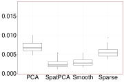
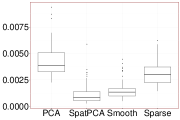
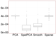
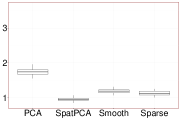
Keywords: Alternating direction method of multipliers, empirical orthogonal functions, fixed rank kriging, Lasso, non-stationary spatial covariance estimation, orthogonal constraint, smoothing splines.

\doublespacing
\doublespacing

1 Introduction

In many atmospheric and earth sciences, it is of interest to identify dominant spatial patterns of variation based on data observed at p𝑝p locations with n𝑛n repeated measurements, where p𝑝p may be larger than n𝑛n. The dominant patterns are the eigenimages of the underlying (nonstationary) spatial covariance function with large eigenvalues. A commonly used approach for estimating the eigenimages is the principal component analysis (PCA), also known as the empirical orthogonal function analysis in atmospheric science. However, when p𝑝p is large relative to n𝑛n, the leading eigenimages produced from PCA may be noisy with high estimation variability, or exhibit some bizarre patterns that are not physically meaningful. To enhance the interpretability, a few approaches, such as rotation of components according to some criteria (see Richman (1986), Jolliffe (1987), Richman (1987)), have been proposed to form more desirable patterns. However, how to obtain a desired rotation in practice is not completely clear. Some discussion can be found in Hannachi, Jolliffe and Stephenson (2007).

Another approach to aid interpretation is to seek sparse or spatially localized patterns, which can be done by imposing an L1subscript𝐿1L_{1} constraint or adding an L1subscript𝐿1L_{1} penalty to an original PCA optimization formulation (Jolliffe, Uddin and Vines (2002), Zou, Hastie and Tibshirani (2006), Shen and Huang (2008), d’Aspremont, Bach and Ghaoui (2008), and Lu and Zhang (2012)). However, this approach may produce a pattern with isolated zero and nonzero components, and except Jolliffe, Uddin and Vines (2002) and Lu and Zhang (2012), the PC estimates produced from these approaches may not have orthogonal PC loadings.

For continuous spatial domains, the problem becomes even more challenging. Instead of looking for eigenimages on a lattice, we need to find eigenfunctions by essentially solving an infinite dimensional problem based on data observed at possibly sparse and irregularly spaced locations. Although some approaches have been developed using functional principal component analysis (see e.g., Ramsay and Silverman (2005), Yao, Muller and Wang (2005) and Huang, Shen and Buja (2008)), they typically focus on one-dimensional processes, or require data observed at dense locations. In particular, these methods generally do not work well when data are observed at fixed but sparse locations. Reviews of PCA on spatial data can be found in Hannachi, Jolliffe and Stephenson (2007) and Demsar et al. (2013).

In this research, we propose a regularization approach for estimating the dominant patterns, taking into account smoothness and localized features that are expected in real-world spatial processes. The proposed estimates are directly obtained by solving a minimization problem. We call our method SpatPCA, which not only gives effective estimates of dominant patterns, but also provides an ideal set of basis functions for estimating the underlying (nonstationary) spatial covariance function, even when data are irregularly or sparsely located in space. In addition, we develop a fast algorithm to solve the resulting optimization problem using the alternating direction method of multipliers (ADMM) (see Boyd et al. (2011)). An R package called SpatPCA is developed and available on the Comprehensive R Archive Network (CRAN).

The rest of this paper is organized as follows. In Section 2, we introduce the proposed SpatPCA method, including dominant patterns estimation and spatial covariance function estimation. Our ADMM algorithm for computing the SpatPCA estimates is provided in Section 3. Some simulation experiments that illustrate the superiority of SpatPCA and an application of SpatPCA to a global sea surface temperature dataset are presented in Section 4.

2 The Proposed Method

Consider a sequence of zero-mean L2superscript𝐿2L^{2}-continuous spatial processes, {ηi(𝒔);𝒔D}subscript𝜂𝑖𝒔𝒔𝐷\{\eta_{i}(\bm{s});\bm{s}\in D\}; i=1,,n𝑖1𝑛i=1,\dots,n, defined on a spatial domain Dd𝐷superscript𝑑D\subset\mathbb{R}^{d}, which are mutually uncorrelated, and have a common spatial covariance function, Cη(𝒔,𝒔)=cov(ηi(𝒔),ηi(𝒔))subscript𝐶𝜂𝒔superscript𝒔covsubscript𝜂𝑖𝒔subscript𝜂𝑖superscript𝒔C_{\eta}(\bm{s},\bm{s}^{*})=\mathrm{cov}(\eta_{i}(\bm{s}),\eta_{i}(\bm{s}^{*})). We consider a rank-K𝐾K spatial random-effects model for ηi()subscript𝜂𝑖\eta_{i}(\cdot):

ηi(𝒔)=(φ1(𝒔),,φK(𝒔))𝝃i=k=1Kξikφk(𝒔);𝒔D,i=1,,n,formulae-sequencesubscript𝜂𝑖𝒔subscript𝜑1𝒔subscript𝜑𝐾𝒔subscript𝝃𝑖superscriptsubscript𝑘1𝐾subscript𝜉𝑖𝑘subscript𝜑𝑘𝒔formulae-sequence𝒔𝐷𝑖1𝑛\eta_{i}(\bm{s})=(\varphi_{1}(\bm{s}),\dots,\varphi_{K}(\bm{s}))\bm{\xi}_{i}=\sum_{k=1}^{K}\xi_{ik}\varphi_{k}(\bm{s});\quad\bm{s}\in D,\quad i=1,\dots,n,

where {φk(.)}\{\varphi_{k}(.)\} are unknown orthonormal basis functions, 𝝃i=(ξi1,,ξiK)(0,𝚲)subscript𝝃𝑖superscriptsubscript𝜉𝑖1subscript𝜉𝑖𝐾similar-to0𝚲\bm{\xi}_{i}=(\xi_{i1},\dots,\xi_{iK})^{\prime}\sim(0,\bm{\Lambda}); i=1,,n𝑖1𝑛i=1,\dots,n, are uncorrelated random variables, and 𝚲𝚲\bm{\Lambda} is an unknown symmetric nonnegative-definite matrix, denoted by 𝚲𝟎succeeds-or-equals𝚲0\bm{\Lambda}\succeq\bm{0}. A similar model based on given {φk()}subscript𝜑𝑘\{\varphi_{k}(\cdot)\} was introduced by Cressie and Johannesson (2008) and in a Bayesian framework by Kang and Cressie (2011).

Let λkksubscript𝜆𝑘superscript𝑘\lambda_{kk^{\prime}} be the (k,k)𝑘superscript𝑘(k,k^{\prime})-th entry of 𝚲𝚲\bm{\Lambda}. Then the spatial covariance function of ηi()subscript𝜂𝑖\eta_{i}(\cdot) is:

Cη(𝒔,𝒔)=cov(ηi(𝒔),ηi(𝒔))=k=1Kk=1Kλkkφk(𝒔)φk(𝒔).subscript𝐶𝜂𝒔superscript𝒔covsubscript𝜂𝑖𝒔subscript𝜂𝑖superscript𝒔superscriptsubscript𝑘1𝐾superscriptsubscriptsuperscript𝑘1𝐾subscript𝜆𝑘superscript𝑘subscript𝜑𝑘𝒔subscript𝜑superscript𝑘superscript𝒔C_{\eta}(\bm{s},\bm{s}^{*})=\mathrm{cov}(\eta_{i}(\bm{s}),\eta_{i}(\bm{s}^{*}))=\sum_{k=1}^{K}\sum_{k^{\prime}=1}^{K}\lambda_{kk^{\prime}}\varphi_{k}(\bm{s})\varphi_{k^{\prime}}(\bm{s}^{*}). (1)

Note that 𝚲𝚲\bm{\Lambda} is not restricted to be a diagonal matrix.

Let 𝚲=𝑽𝚲𝑽𝚲𝑽superscript𝚲superscript𝑽\bm{\Lambda}=\bm{V}\bm{\Lambda^{*}}\bm{V}^{\prime} be the eigen-decomposition of 𝚲𝚲\bm{\Lambda}, where 𝑽𝑽\bm{V} consists of K𝐾K orthonormal eigenvectors, and 𝚲=diag(λ1,,λK)superscript𝚲diagsubscriptsuperscript𝜆1subscriptsuperscript𝜆𝐾\bm{\Lambda}^{*}=\mathrm{diag}(\lambda^{*}_{1},\dots,\lambda^{*}_{K}) consists of eigenvalues with λ1λKsubscriptsuperscript𝜆1subscriptsuperscript𝜆𝐾\lambda^{*}_{1}\geq\cdots\geq\lambda^{*}_{K}. Let 𝝃i=𝑽𝝃isubscriptsuperscript𝝃𝑖superscript𝑽subscript𝝃𝑖\bm{\xi}^{*}_{i}=\bm{V}^{\prime}\bm{\xi}_{i} and

(φ1(𝒔),,φK(𝒔))=(φ1(𝒔),,φK(𝒔))𝑽;𝒔D.formulae-sequencesubscriptsuperscript𝜑1𝒔subscriptsuperscript𝜑𝐾𝒔subscript𝜑1𝒔subscript𝜑𝐾𝒔𝑽𝒔𝐷(\varphi^{*}_{1}(\bm{s}),\dots,\varphi^{*}_{K}(\bm{s}))=(\varphi_{1}(\bm{s}),\dots,\varphi_{K}(\bm{s}))\bm{V};\quad\bm{s}\in D.

Then φk()subscriptsuperscript𝜑𝑘\varphi^{*}_{k}(\cdot)’s are also orthonormal, and ξik(0,λk)similar-tosubscriptsuperscript𝜉𝑖𝑘0subscriptsuperscript𝜆𝑘\xi^{*}_{ik}\sim(0,\lambda^{*}_{k}); i=1,,n,k=1,,Kformulae-sequence𝑖1𝑛𝑘1𝐾i=1,\dots,n,\,k=1,\dots,K, are mutually uncorrelated. Therefore, we can rewrite ηi()subscript𝜂𝑖\eta_{i}(\cdot) in terms of φk()subscriptsuperscript𝜑𝑘\varphi^{*}_{k}(\cdot)’s:

ηi(𝒔)=(φ1(𝒔),,φK(𝒔))𝝃i=k=1Kξikφk(𝒔);𝒔D.formulae-sequencesubscript𝜂𝑖𝒔subscriptsuperscript𝜑1𝒔subscriptsuperscript𝜑𝐾𝒔subscriptsuperscript𝝃𝑖superscriptsubscript𝑘1𝐾subscriptsuperscript𝜉𝑖𝑘subscriptsuperscript𝜑𝑘𝒔𝒔𝐷\eta_{i}(\bm{s})=(\varphi^{*}_{1}(\bm{s}),\dots,\varphi^{*}_{K}(\bm{s}))\bm{\xi}^{*}_{i}=\sum_{k=1}^{K}\xi^{*}_{ik}\varphi^{*}_{k}(\bm{s});\quad\bm{s}\in D. (2)

The above expansion is known as the Karhunen-Loéve expansion of ηi()subscript𝜂𝑖\eta_{i}(\cdot) (Karhunen (1947); Loève (1978)) with K𝐾K nonzero eigenvalues, where φk()subscriptsuperscript𝜑𝑘\varphi^{*}_{k}(\cdot) is the k𝑘k-th eigenfunction of Cη(,)subscript𝐶𝜂C_{\eta}(\cdot,\cdot) with λksubscriptsuperscript𝜆𝑘\lambda^{*}_{k} the corresponding eigenvalue.

Suppose that we observe data 𝒀i=(Yi(𝒔1),,Yi(𝒔p))subscript𝒀𝑖superscriptsubscript𝑌𝑖subscript𝒔1subscript𝑌𝑖subscript𝒔𝑝\bm{Y}_{i}=(Y_{i}(\bm{s}_{1}),\dots,Y_{i}(\bm{s}_{p}))^{\prime} with added white noise ϵi(𝟎,σ2𝑰)similar-tosubscriptbold-italic-ϵ𝑖0superscript𝜎2𝑰\bm{\epsilon}_{i}\sim(\bm{0},\sigma^{2}\bm{I}) at p𝑝p spatial locations, 𝒔1,,𝒔pDsubscript𝒔1subscript𝒔𝑝𝐷\bm{s}_{1},\dots,\bm{s}_{p}\in D, according to

𝒀i=𝜼i+ϵi=𝚽𝝃i+ϵi;i=1,,n,formulae-sequencesubscript𝒀𝑖subscript𝜼𝑖subscriptbold-italic-ϵ𝑖𝚽subscript𝝃𝑖subscriptbold-italic-ϵ𝑖𝑖1𝑛\bm{Y}_{i}=\bm{\eta}_{i}+\bm{\epsilon}_{i}=\bm{\Phi}\bm{\xi}_{i}+\bm{\epsilon}_{i};\quad i=1,\dots,n, (3)

where 𝜼i=(ηi(𝒔1),,ηi(𝒔p))subscript𝜼𝑖superscriptsubscript𝜂𝑖subscript𝒔1subscript𝜂𝑖subscript𝒔𝑝\bm{\eta}_{i}=(\eta_{i}(\bm{s}_{1}),\dots,\eta_{i}(\bm{s}_{p}))^{\prime}, 𝚽=(ϕ1,,ϕK)𝚽subscriptbold-italic-ϕ1subscriptbold-italic-ϕ𝐾\bm{\Phi}=(\bm{\phi}_{1},\dots,\bm{\phi}_{K}) is a p×K𝑝𝐾p\times K matrix with the (j,k)𝑗𝑘(j,k)-th entry φk(𝒔j)subscript𝜑𝑘subscript𝒔𝑗\varphi_{k}(\bm{s}_{j}), and ϵisubscriptbold-italic-ϵ𝑖\bm{\epsilon}_{i}’s and 𝝃isubscript𝝃𝑖\bm{\xi}_{i}’s are uncorrelated. Our goal is to identify the first LK𝐿𝐾L\leq K dominant patterns, φ1(),,φL()subscript𝜑1subscript𝜑𝐿\varphi_{1}(\cdot),\dots,\varphi_{L}(\cdot), with relatively large λ1,,λLsubscriptsuperscript𝜆1subscriptsuperscript𝜆𝐿\lambda^{*}_{1},\dots,\lambda^{*}_{L}. Additionally, we are interested in estimating Cη(,)subscript𝐶𝜂C_{\eta}(\cdot,\cdot), which is essential for spatial prediction.

Let 𝒀=(𝒀1,,𝒀n)𝒀superscriptsubscript𝒀1subscript𝒀𝑛\bm{Y}=(\bm{Y}_{1},\dots,\bm{Y}_{n})^{\prime} be the n×p𝑛𝑝n\times p data matrix. Throughout the paper, we assume that the mean of 𝒀𝒀\bm{Y} is known as zero. So the sample covariance matrix of 𝒀𝒀\bm{Y} is 𝑺=𝒀𝒀/n𝑺superscript𝒀𝒀𝑛\bm{S}=\bm{Y}^{\prime}\bm{Y}/n. A popular approach for estimating {φk()}subscriptsuperscript𝜑𝑘\{\varphi^{*}_{k}(\cdot)\} is PCA, which estimates (φk(𝒔1),,φk(𝒔p))superscriptsubscriptsuperscript𝜑𝑘subscript𝒔1subscriptsuperscript𝜑𝑘subscript𝒔𝑝(\varphi^{*}_{k}(\bm{s}_{1}),\dots,\varphi^{*}_{k}(\bm{s}_{p}))^{\prime} by ϕ~ksubscript~bold-italic-ϕ𝑘\tilde{\bm{\phi}}_{k}, the k𝑘k-th eigenvector of 𝑺𝑺\bm{S}, for k=1,,K𝑘1𝐾k=1,\dots,K. Let 𝚽~=(ϕ~1,,ϕ~K)~𝚽subscript~bold-italic-ϕ1subscript~bold-italic-ϕ𝐾\tilde{\bm{\Phi}}=\big{(}\tilde{\bm{\phi}}_{1},\dots,\tilde{\bm{\phi}}_{K}\big{)} be a p×K𝑝𝐾p\times K matrix formed by the first K𝐾K principal component loadings. Then 𝚽~~𝚽\tilde{\bm{\Phi}} solves the following constrained optimization problem:

min𝚽𝒀𝒀𝚽𝚽F2subject to 𝚽𝚽=𝑰K,subscript𝚽subscriptsuperscriptnorm𝒀𝒀𝚽superscript𝚽2𝐹subject to superscript𝚽𝚽subscript𝑰𝐾\min_{\bm{\Phi}}\|\bm{Y}-\bm{Y}\bm{\Phi}\bm{\Phi}^{\prime}\|^{2}_{F}\quad\text{subject to }\bm{\Phi}^{\prime}\bm{\Phi}=\bm{I}_{K},

where 𝚽=(ϕ1,,ϕK)𝚽subscriptbold-italic-ϕ1subscriptbold-italic-ϕ𝐾\bm{\Phi}=(\bm{\phi}_{1},\dots,\bm{\phi}_{K}) and 𝑴F=(i,jmij2)1/2subscriptnorm𝑴𝐹superscriptsubscript𝑖𝑗subscriptsuperscript𝑚2𝑖𝑗12\|\bm{M}\|_{F}=\Big{(}\displaystyle\sum_{i,j}m^{2}_{ij}\Big{)}^{1/2} is the Frobenius norm of a matrix 𝑴𝑴\bm{M}. Unfortunately, 𝚽~~𝚽\tilde{\bm{\Phi}} tends to have high estimation variability when p𝑝p is large (leading to excessive number of parameters), n𝑛n is small, or σ2superscript𝜎2\sigma^{2} is large. Consequently, the patterns of 𝚽~~𝚽\tilde{\bm{\Phi}} may be too noisy to be physically interpretable. In addition, for a continuous spatial domain D𝐷D, we also need to estimate φk(𝒔)superscriptsubscript𝜑𝑘𝒔\varphi_{k}^{*}(\bm{s})’s for locations with no data observed (i.e., 𝒔{𝒔1,,𝒔p}𝒔subscript𝒔1subscript𝒔𝑝\bm{s}\notin\{\bm{s}_{1},\dots,\bm{s}_{p}\}); see some discussion in Section 12.4 and 13.6 of Jolliffe (2002).

2.1 Regularized Spatial PCA

To prevent high estimation variability of PCA, we adopt a regularization approach by minimizing the following objective function:

𝒀𝒀𝚽𝚽F2+τ1k=1KJ(φk)+τ2k=1Kj=1p|φk(𝒔j)|,subscriptsuperscriptnorm𝒀𝒀𝚽superscript𝚽2𝐹subscript𝜏1superscriptsubscript𝑘1𝐾𝐽subscript𝜑𝑘subscript𝜏2superscriptsubscript𝑘1𝐾superscriptsubscript𝑗1𝑝subscript𝜑𝑘subscript𝒔𝑗\|\bm{Y}-\bm{Y}\bm{\Phi}\bm{\Phi}^{\prime}\|^{2}_{F}+\tau_{1}\sum_{k=1}^{K}J({\varphi}_{k})+\tau_{2}\sum_{k=1}^{K}\sum_{j=1}^{p}\big{|}\varphi_{k}(\bm{s}_{j})\big{|}, (4)

over φ1(),,φK()subscript𝜑1subscript𝜑𝐾\varphi_{1}(\cdot),\dots,\varphi_{K}(\cdot), subject to 𝚽𝚽=𝑰Ksuperscript𝚽𝚽subscript𝑰𝐾\bm{\Phi}^{\prime}\bm{\Phi}=\bm{I}_{K} and ϕ1𝑺ϕ1ϕ2𝑺ϕ2ϕK𝑺ϕKsubscriptsuperscriptbold-italic-ϕ1𝑺subscriptbold-italic-ϕ1subscriptsuperscriptbold-italic-ϕ2𝑺subscriptbold-italic-ϕ2subscriptsuperscriptbold-italic-ϕ𝐾𝑺subscriptbold-italic-ϕ𝐾\bm{\phi}^{\prime}_{1}\bm{S}\bm{\phi}_{1}\geq\bm{\phi}^{\prime}_{2}\bm{S}\bm{\phi}_{2}\geq\cdots\geq\bm{\phi}^{\prime}_{K}\bm{S}\bm{\phi}_{K}, where

J(φ)=z1++zd=2d(2φ(𝒔)x1z1xdzd)2𝑑𝒔,𝐽𝜑subscriptsubscript𝑧1subscript𝑧𝑑2subscriptsuperscript𝑑superscriptsuperscript2𝜑𝒔superscriptsubscript𝑥1subscript𝑧1superscriptsubscript𝑥𝑑subscript𝑧𝑑2differential-d𝒔J(\varphi)=\sum_{z_{1}+\cdots+z_{d}=2}\int_{\mathcal{R}^{d}}\left(\frac{\partial^{2}\varphi(\bm{s})}{\partial x_{1}^{z_{1}}\dots\partial x_{d}^{z_{d}}}\right)^{2}d\bm{s},

is a roughness penalty, 𝒔=(x1,,xd)𝒔superscriptsubscript𝑥1subscript𝑥𝑑\bm{s}=(x_{1},\dots,x_{d})^{\prime}, τ10subscript𝜏10\tau_{1}\geq 0 is a smoothness parameter, and τ20subscript𝜏20\tau_{2}\geq 0 is a sparseness parameter. The objective function (4) consists of two penalty terms. The first one is designed to enhance smoothness of φk()subscript𝜑𝑘\varphi_{k}(\cdot) through the smoothing spline penalty J(φk)𝐽subscript𝜑𝑘J(\varphi_{k}), while the second one is the L1subscript𝐿1L_{1} Lasso penalty (Tibshirani (1996)), used to promote sparse patterns by shrinking some PC loadings to zero. While the L1subscript𝐿1L_{1} penalty alone may lead to isolated zero and nonzero components with no global feature, when it is paired with the smoothness penalty, local sparsity translates into global sparsity, resulting in connected zero and nonzero patterns. Hence the two penalty terms together lead to desired patterns that are not only smooth but also localized. Specifically, when τ1subscript𝜏1\tau_{1} is larger, φ^k()subscript^𝜑𝑘\hat{\varphi}_{k}(\cdot)’s tend to be smoother and vice versa. When τ2subscript𝜏2\tau_{2} is larger, φ^k()subscript^𝜑𝑘\hat{\varphi}_{k}(\cdot)’s are forced to be zero at some 𝒔D𝒔𝐷\bm{s}\in D. On the other hand, when both τ1subscript𝜏1\tau_{1} and τ2subscript𝜏2\tau_{2} are close to zero, the estimates are close to those obtained from PCA. By suitably choosing τ1subscript𝜏1\tau_{1} and τ2subscript𝜏2\tau_{2}, we can obtain a good compromise among goodness of fit, smoothness of the eigenfunctions, and sparseness of the eigenfunctions, leading to more interpretable results. Note that due to computational difficulty, the orthogonal constraint, is not considered by many PCA regularization methods (e.g., Zou, Hastie and Tibshirani (2006), Shen and Huang (2008), Guo et al. (2010), Hong and Lian (2013)).

Although J(φ)𝐽𝜑J(\varphi) involves integration, it is well known from the theory of smoothing splines (Green and Silverman (1994)) that for each k=1,,K𝑘1𝐾k=1,\dots,K, φ^k()subscript^𝜑𝑘\hat{\varphi}_{k}(\cdot) has to be a natural cubic spline when d=1𝑑1d=1, and a thin-plate spline when d{2,3}𝑑23d\in\{2,3\} with nodes at {𝒔1,,𝒔p}subscript𝒔1subscript𝒔𝑝\{\bm{s}_{1},\dots,\bm{s}_{p}\}. Specifically,

φ^k(𝒔)=i=1paig(𝒔𝒔i)+b0+j=1dbjxj,subscript^𝜑𝑘𝒔superscriptsubscript𝑖1𝑝subscript𝑎𝑖𝑔norm𝒔subscript𝒔𝑖subscript𝑏0superscriptsubscript𝑗1𝑑subscript𝑏𝑗subscript𝑥𝑗\hat{\varphi}_{k}(\bm{s})=\sum_{i=1}^{p}{a}_{i}g(\|\bm{s}-\bm{s}_{i}\|)+b_{0}+\sum_{j=1}^{d}{b}_{j}x_{j}\>, (5)

where 𝒔=(x1,,xd)𝒔superscriptsubscript𝑥1subscript𝑥𝑑\bm{s}=(x_{1},\dots,x_{d})^{\prime},

g(r)={116πr2logr;if d=2,Γ(d/22)16πd/2r4d;if d=1,3,𝑔𝑟cases116𝜋superscript𝑟2𝑟if d=2,Γ𝑑2216superscript𝜋𝑑2superscript𝑟4𝑑if 𝑑13g(r)=\left\{\begin{array}[]{ll}\displaystyle\frac{1}{16\pi}r^{2}\log{r};&\mbox{if $d=2$,}\vskip 3.0pt plus 1.0pt minus 1.0pt\\ \displaystyle\frac{\Gamma(d/2-2)}{16\pi^{d/2}}r^{4-d};&\mbox{if }d=1,3,\\ \end{array}\right.

and the coefficients 𝒂=(a1,,ap)𝒂superscriptsubscript𝑎1subscript𝑎𝑝{\bm{a}}=\left({a}_{1},\dots,{a}_{p}\right)^{\prime} and 𝒃=(b0,b1,,bd)𝒃superscriptsubscript𝑏0subscript𝑏1subscript𝑏𝑑{\bm{b}}=\left({b}_{0},b_{1},\dots,{b}_{d}\right)^{\prime} satisfy

[𝑮𝑬𝑬T𝟎][𝒂𝒃]=[ϕ^k𝟎].matrix𝑮𝑬superscript𝑬𝑇0matrix𝒂𝒃matrixsubscript^bold-italic-ϕ𝑘0\begin{bmatrix}\bm{G}&\bm{E}\\ \bm{E}^{T}&\bm{0}\\ \end{bmatrix}\begin{bmatrix}{\bm{a}}\\ {\bm{b}}\end{bmatrix}=\begin{bmatrix}\hat{\bm{\phi}}_{k}\\ \bm{0}\end{bmatrix}.

Here 𝑮𝑮\bm{G} is a p×p𝑝𝑝p\times p matrix with the (i,j)𝑖𝑗(i,j)-th element g(𝒔i𝒔j)𝑔normsubscript𝒔𝑖subscript𝒔𝑗g(\|\bm{s}_{i}-\bm{s}_{j}\|), and 𝑬𝑬\bm{E} is a p×(d+1)𝑝𝑑1p\times(d+1) matrix with the i𝑖i-th row (1,𝒔i)1subscriptsuperscript𝒔𝑖(1,\bm{s}^{\prime}_{i}). Consequently, φ^k()subscript^𝜑𝑘\hat{\varphi}_{k}(\cdot) in (5) can be expressed in terms of ϕ^ksubscript^bold-italic-ϕ𝑘\hat{\bm{\phi}}_{k}. Additionally, the roughness penalty can also be written as

J(φk)=ϕk𝛀ϕk,𝐽subscript𝜑𝑘subscriptsuperscriptbold-italic-ϕ𝑘𝛀subscriptbold-italic-ϕ𝑘J(\varphi_{k})=\bm{\phi}^{\prime}_{k}\bm{\Omega}\bm{\phi}_{k}, (6)

with 𝛀𝛀\bm{\Omega} a known p×p𝑝𝑝p\times p matrix determined only by 𝒔1,,𝒔psubscript𝒔1subscript𝒔𝑝\bm{s}_{1},\dots,\bm{s}_{p}. The readers are referred to Green and Silverman (1994) for more details regarding smoothing splines.

From (4) and (6), the proposed SpatPCA estimate of 𝚽𝚽\bm{\Phi} can be written as:

𝚽^τ1,τ2=argmin𝚽:𝚽𝚽=𝑰K𝒀𝒀𝚽𝚽F2+τ1k=1Kϕk𝛀ϕk+τ2k=1Kj=1p|ϕjk|,subscript^𝚽subscript𝜏1subscript𝜏2subscript:𝚽superscript𝚽𝚽subscript𝑰𝐾subscriptsuperscriptnorm𝒀𝒀𝚽superscript𝚽2𝐹subscript𝜏1superscriptsubscript𝑘1𝐾subscriptsuperscriptbold-italic-ϕ𝑘𝛀subscriptbold-italic-ϕ𝑘subscript𝜏2superscriptsubscript𝑘1𝐾superscriptsubscript𝑗1𝑝subscriptitalic-ϕ𝑗𝑘\hat{\bm{\Phi}}_{\tau_{1},\tau_{2}}=\mathop{\arg\min}_{\bm{\Phi}:\bm{\Phi}^{\prime}\bm{\Phi}=\bm{I}_{K}}\|\bm{Y}-\bm{Y}\bm{\Phi}\bm{\Phi}^{\prime}\|^{2}_{F}+\tau_{1}\sum_{k=1}^{K}\bm{\phi}^{\prime}_{k}\bm{\Omega}\bm{\phi}_{k}+\tau_{2}\sum_{k=1}^{K}\sum_{j=1}^{p}\left|{\phi}_{jk}\right|, (7)

subject to ϕ1𝑺ϕ1ϕ2𝑺ϕ2ϕK𝑺ϕKsubscriptsuperscriptbold-italic-ϕ1𝑺subscriptbold-italic-ϕ1subscriptsuperscriptbold-italic-ϕ2𝑺subscriptbold-italic-ϕ2subscriptsuperscriptbold-italic-ϕ𝐾𝑺subscriptbold-italic-ϕ𝐾\bm{\phi}^{\prime}_{1}\bm{S}\bm{\phi}_{1}\geq\bm{\phi}^{\prime}_{2}\bm{S}\bm{\phi}_{2}\geq\cdots\geq\bm{\phi}^{\prime}_{K}\bm{S}\bm{\phi}_{K}. The resulting estimates of φ1(),,φK()subscript𝜑1subscript𝜑𝐾\varphi_{1}(\cdot),\dots,\varphi_{K}(\cdot) can be directly computed from (5). When no confusion may arise, we shall simply write 𝚽^τ1,τ2subscript^𝚽subscript𝜏1subscript𝜏2\hat{\bm{\Phi}}_{\tau_{1},\tau_{2}} as 𝚽^^𝚽\hat{\bm{\Phi}}. Note that the SpatPCA estimate of (7) reduces to a sparse PCA estimate of Zou, Hastie and Tibshirani (2006) if the orthogonal constraint is dropped and 𝛀=𝑰𝛀𝑰\bm{\Omega}=\bm{I} (i.e., no spatial structure is considered).

The tuning parameters τ1subscript𝜏1\tau_{1} and τ2subscript𝜏2\tau_{2} are selected using M𝑀M-fold cross-validation (CV). First, we partition {1,,n}1𝑛\{1,\dots,n\} into M𝑀M parts with as close to the same size as possible. Let 𝒀(m)superscript𝒀𝑚\bm{Y}^{(m)} be the sub-matrix of 𝒀𝒀\bm{Y} corresponding to the m𝑚m-th part, for m=1,,M𝑚1𝑀m=1,\dots,M. For each part, we treat 𝒀(m)superscript𝒀𝑚\bm{Y}^{(m)} as the validation data, and obtain the estimate 𝚽^τ1,τ2(m)subscriptsuperscript^𝚽𝑚subscript𝜏1subscript𝜏2\hat{\bm{\Phi}}^{(-m)}_{\tau_{1},\tau_{2}} of 𝚽𝚽\bm{\Phi} for (τ1,τ2)𝒜subscript𝜏1subscript𝜏2𝒜(\tau_{1},\tau_{2})\in\mathcal{A} based on the remaining data 𝒀(m)superscript𝒀𝑚\bm{Y}^{(-m)} using the proposed method, where 𝒜[0,)2𝒜superscript02\mathcal{A}\subset[0,\infty)^{2} is a candidate index set. The proposed CV criterion is given in terms of an average residual sum of squares:

CV1(τ1,τ2)=1Mm=1M𝒀(m)𝒀(m)𝚽^τ1,τ2(m)(𝚽^τ1,τ2(m))F2,subscriptCV1subscript𝜏1subscript𝜏21𝑀superscriptsubscript𝑚1𝑀subscriptsuperscriptnormsuperscript𝒀𝑚superscript𝒀𝑚superscriptsubscript^𝚽subscript𝜏1subscript𝜏2𝑚superscriptsubscriptsuperscript^𝚽𝑚subscript𝜏1subscript𝜏22𝐹\mathrm{CV}_{1}(\tau_{1},\tau_{2})=\frac{1}{M}\sum_{m=1}^{M}\big{\|}\bm{Y}^{(m)}-\bm{Y}^{(m)}\hat{\bm{\Phi}}_{\tau_{1},\tau_{2}}^{(-m)}(\hat{\bm{\Phi}}^{(-m)}_{\tau_{1},\tau_{2}})^{\prime}\big{\|}^{2}_{F}\>, (8)

where 𝒀(m)𝚽^τ1,τ2(m)(𝚽^τ1,τ2(m))superscript𝒀𝑚superscriptsubscript^𝚽subscript𝜏1subscript𝜏2𝑚superscriptsubscriptsuperscript^𝚽𝑚subscript𝜏1subscript𝜏2\bm{Y}^{(m)}\hat{\bm{\Phi}}_{\tau_{1},\tau_{2}}^{(-m)}(\hat{\bm{\Phi}}^{(-m)}_{\tau_{1},\tau_{2}})^{\prime} is the projection of 𝒀(m)superscript𝒀𝑚\bm{Y}^{(m)} onto the column space of 𝚽^τ1,τ2(m)subscriptsuperscript^𝚽𝑚subscript𝜏1subscript𝜏2\hat{\bm{\Phi}}^{(-m)}_{\tau_{1},\tau_{2}}. The final τ1subscript𝜏1\tau_{1} and τ2subscript𝜏2\tau_{2} values are (τ^1,τ^2)=argmin(τ1,τ2)𝒜CV1(τ1,τ2)subscript^𝜏1subscript^𝜏2subscriptsubscript𝜏1subscript𝜏2𝒜subscriptCV1subscript𝜏1subscript𝜏2(\hat{\tau}_{1},\hat{\tau}_{2})=\displaystyle\mathop{\arg\min}_{(\tau_{1},\tau_{2})\in\mathcal{A}}\mathrm{CV}_{1}(\tau_{1},\tau_{2}).

2.2 Estimation of Spatial Covariance Function

To estimate Cη(,)subscript𝐶𝜂C_{\eta}(\cdot,\cdot) in (1), we also need to estimate the spatial covariance parameters, σ2superscript𝜎2\sigma^{2} and 𝚲𝚲\bm{\Lambda}. We apply the regularized least squares method of Tzeng and Huang (2015):

(σ^2,𝚲^)=argmin(σ2,𝚲):σ20,𝚲𝟎{12𝑺𝚽^𝚲𝚽^σ2𝑰F2+γ𝚽^𝚲𝚽^},superscript^𝜎2^𝚲subscript:superscript𝜎2𝚲formulae-sequencesuperscript𝜎20succeeds-or-equals𝚲0conditional-set12𝑺^𝚽𝚲superscript^𝚽evaluated-atsuperscript𝜎2𝑰𝐹2𝛾subscriptnorm^𝚽𝚲superscript^𝚽\big{(}\hat{\sigma}^{2},\hat{\bm{\Lambda}}\big{)}=\mathop{\arg\min}_{(\sigma^{2},\bm{\Lambda}):\sigma^{2}\geq 0,\,\bm{\Lambda}\succeq\bm{0}}\bigg{\{}\frac{1}{2}\big{\|}\bm{S}-\hat{\bm{\Phi}}\bm{\Lambda}\hat{\bm{\Phi}}^{\prime}-\sigma^{2}\bm{I}\big{\|}^{2}_{F}+\gamma\|\hat{\bm{\Phi}}\bm{\Lambda}\hat{\bm{\Phi}}^{\prime}\|_{*}\bigg{\}}, (9)

where γ0𝛾0\gamma\geq 0 is a tuning parameter, and 𝑴=tr((𝑴𝑴)1/2)subscriptnorm𝑴trsuperscriptsuperscript𝑴𝑴12\|\bm{M}\|_{*}=\mathrm{tr}((\bm{M}^{\prime}\bm{M})^{1/2}) is the nuclear norm of 𝑴𝑴\bm{M}. The first term of (9) corresponds to goodness of fit by noting that var(𝒀i)=𝚽𝚲𝚽+σ2𝑰varsubscript𝒀𝑖𝚽𝚲superscript𝚽superscript𝜎2𝑰\mathrm{var}(\bm{Y}_{i})=\bm{\Phi\Lambda\Phi}^{\prime}+\sigma^{2}\bm{I}. The second term of (9) is a convex penalty, shrinking the eigenvalues of 𝚽^𝚲𝚽^^𝚽𝚲superscript^𝚽\hat{\bm{\Phi}}\bm{\Lambda}\hat{\bm{\Phi}}^{\prime} to promote a low-rank structure and to avoid the eigenvalues being overestimated. By suitably choosing a tuning parameter γ𝛾\gamma, we can control the bias, while reducing the estimation variability. This is particularly effective when K𝐾K is large.

Tzeng and Huang (2015) provides a closed-form solution for 𝚲^^𝚲\hat{\bm{\Lambda}}, but requires an iterative procedure for solving σ^2superscript^𝜎2\hat{\sigma}^{2}. We found that closed-form expressions for both σ^2superscript^𝜎2\hat{\sigma}^{2} and 𝚲^^𝚲\hat{\bm{\Lambda}} are available, and are shown in the following proposition with its proof given in the Appendix.

Proposition 1.

The solutions of (9) are given by

𝚲^=^𝚲absent\displaystyle\hat{\bm{\Lambda}}= 𝑽^diag(λ^1,,λ^K)𝑽^,^𝑽diagsuperscriptsubscript^𝜆1superscriptsubscript^𝜆𝐾superscript^𝑽\displaystyle~{}\hat{\bm{V}}\mathrm{diag}\big{(}\hat{\lambda}_{1}^{*},\dots,\hat{\lambda}_{K}^{*}\big{)}\hat{\bm{V}}^{\prime}, (10)
σ^2=superscript^𝜎2absent\displaystyle\hat{\sigma}^{2}= {1pL^(tr(𝑺)k=1L^(d^kγ));if d^1>γ,1p(tr(𝑺));if d^1γ ,cases1𝑝^𝐿tr𝑺superscriptsubscript𝑘1^𝐿subscript^𝑑𝑘𝛾if d^1>γ,1𝑝tr𝑺if d^1γ ,\displaystyle~{}\left\{\begin{array}[]{ll}\displaystyle\frac{1}{p-\hat{L}}\bigg{(}\mathrm{tr}(\bm{S})-\sum_{k=1}^{\hat{L}}\big{(}\hat{d}_{k}-\gamma\big{)}\bigg{)};&\mbox{if $\hat{d}_{1}>\gamma$,}\\ \displaystyle\frac{1}{p}\left(\mathrm{tr}(\bm{S})\right);&\mbox{if $\hat{d}_{1}\leq\gamma$ ,}\\ \end{array}\right. (13)

where 𝑽^diag(d^1,,d^K)𝑽^^𝑽diagsubscript^𝑑1subscript^𝑑𝐾superscript^𝑽\hat{\bm{V}}\mathrm{diag}(\hat{d}_{1},\dots,\hat{d}_{K})\hat{\bm{V}}^{\prime} is the eigen-decomposition of 𝚽^𝑺𝚽^superscript^𝚽𝑺^𝚽\hat{\bm{\Phi}}^{\prime}\bm{S}\hat{\bm{\Phi}} with d^1d^Ksubscript^𝑑1subscript^𝑑𝐾\hat{d}_{1}\geq\cdots\geq\hat{d}_{K},

L^=max{L:d^Lγ>1pL(tr(𝑺)k=1L(d^kγ)),L=1,,K},^𝐿:𝐿formulae-sequencesubscript^𝑑𝐿𝛾1𝑝𝐿tr𝑺superscriptsubscript𝑘1𝐿subscript^𝑑𝑘𝛾𝐿1𝐾\hat{L}=\max\bigg{\{}L:\hat{d}_{L}-\gamma>\frac{1}{p-L}\bigg{(}\mathrm{tr}(\bm{S})-\sum_{k=1}^{L}(\hat{d}_{k}-\gamma)\bigg{)},L=1,\dots,K\bigg{\}}, (14)

and λ^k=max(d^kσ^2γ,0)subscriptsuperscript^𝜆𝑘subscript^𝑑𝑘superscript^𝜎2𝛾0\hat{\lambda}^{*}_{k}=\max(\hat{d}_{k}-\hat{\sigma}^{2}-\gamma,0); k=1,,K𝑘1𝐾k=1,\dots,K.

With 𝚲^=(λ^kk)K×K^𝚲subscriptsubscript^𝜆𝑘superscript𝑘𝐾𝐾\hat{\bm{\Lambda}}=\big{(}\hat{\lambda}_{kk^{\prime}}\big{)}_{K\times K} given by (9) and φ^k(𝒔)subscript^𝜑𝑘𝒔\hat{\varphi}_{k}(\bm{s}) given by (5), the proposed estimate of Cη(𝒔,𝒔)subscript𝐶𝜂𝒔superscript𝒔C_{\eta}(\bm{s},\bm{s}^{*}) is

C^η(𝒔,𝒔)=k=1Kk=1Kλ^kkφ^k(𝒔)φ^k(𝒔).subscript^𝐶𝜂𝒔superscript𝒔superscriptsubscript𝑘1𝐾superscriptsubscriptsuperscript𝑘1𝐾subscript^𝜆𝑘superscript𝑘subscript^𝜑𝑘𝒔subscript^𝜑superscript𝑘superscript𝒔\hat{C}_{\eta}(\bm{s},\bm{s}^{*})=\sum_{k=1}^{K}\sum_{k^{\prime}=1}^{K}\hat{\lambda}_{kk^{\prime}}\,\hat{\varphi}_{k}(\bm{s})\hat{\varphi}_{k^{\prime}}(\bm{s}^{*}). (15)

Then the proposed estimate of (φ1(𝒔),,φK(𝒔))subscriptsuperscript𝜑1𝒔subscriptsuperscript𝜑𝐾𝒔(\varphi^{*}_{1}(\bm{s}),\dots,\varphi^{*}_{K}(\bm{s})) is

(φ^1(𝒔),,φ^K(𝒔))=(φ^1(𝒔),,φ^K(𝒔))𝑽^;𝒔D.formulae-sequencesubscriptsuperscript^𝜑1𝒔subscriptsuperscript^𝜑𝐾𝒔subscript^𝜑1𝒔subscript^𝜑𝐾𝒔^𝑽𝒔𝐷(\hat{\varphi}^{*}_{1}(\bm{s}),\dots,\hat{\varphi}^{*}_{K}(\bm{s}))=(\hat{\varphi}_{1}(\bm{s}),\dots,\hat{\varphi}_{K}(\bm{s}))\hat{\bm{V}};\quad\bm{s}\in D.

We consider M𝑀M-fold CV to select γ𝛾\gamma. As in the previous section, we partition the data into M𝑀M parts, 𝒀(1),,𝒀(M)superscript𝒀1superscript𝒀𝑀\bm{Y}^{(1)},\dots,\bm{Y}^{(M)}. For m=1,,M𝑚1𝑀m=1,\dots,M, we estimate var(𝒀(m))varsuperscript𝒀𝑚\mathrm{var}\big{(}\bm{Y}^{(-m)}\big{)} by 𝚺^(m)=𝚽^(m)𝚲^γ(m)(𝚽^(m))+(σ^γ2)(m)𝑰superscript^𝚺𝑚superscript^𝚽𝑚subscriptsuperscript^𝚲𝑚𝛾superscriptsuperscript^𝚽𝑚superscriptsubscriptsuperscript^𝜎2𝛾𝑚𝑰\hat{\bm{\Sigma}}^{(-m)}=\hat{\bm{\Phi}}^{(-m)}\hat{\bm{\Lambda}}^{(-m)}_{\gamma}\big{(}\hat{\bm{\Phi}}^{(-m)}\big{)}^{\prime}+\big{(}\hat{\sigma}^{2}_{\gamma}\big{)}^{(-m)}\bm{I} based on the remaining data 𝒀(m)superscript𝒀𝑚\bm{Y}^{(-m)} by removing 𝒀(m)superscript𝒀𝑚\bm{Y}^{(m)} from 𝒀𝒀\bm{Y}, where 𝚲^γ(m)subscriptsuperscript^𝚲𝑚𝛾\hat{\bm{\Lambda}}^{(-m)}_{\gamma}, (σ^γ2)(m)superscriptsubscriptsuperscript^𝜎2𝛾𝑚\big{(}\hat{\sigma}^{2}_{\gamma}\big{)}^{(-m)} and 𝚽^(m)superscript^𝚽𝑚\hat{\bm{\Phi}}^{(-m)} are the estimates of 𝚲𝚲\bm{\Lambda}, σ2superscript𝜎2\sigma^{2} and 𝚽𝚽\bm{\Phi} based on 𝒀(m)superscript𝒀𝑚\bm{Y}^{(-m)}, and for notational simplicity, their dependences on the selected (τ1,τ2)subscript𝜏1subscript𝜏2(\tau_{1},\tau_{2}) and K𝐾K are suppressed. The proposed CV criterion is given by

CV2(K,γ)=1Mm=1M𝑺(m)𝚽^(m)𝚲^γ(m)(𝚽^(m))(σ^γ2)(m)𝑰F2,subscriptCV2𝐾𝛾1𝑀superscriptsubscript𝑚1𝑀subscriptsuperscriptnormsuperscript𝑺𝑚superscript^𝚽𝑚subscriptsuperscript^𝚲𝑚𝛾superscriptsuperscript^𝚽𝑚superscriptsuperscriptsubscript^𝜎𝛾2𝑚𝑰2𝐹\mathrm{CV}_{2}(K,\gamma)=\frac{1}{M}\sum_{m=1}^{M}\big{\|}\bm{S}^{(m)}-\hat{\bm{\Phi}}^{(-m)}\hat{\bm{\Lambda}}^{(-m)}_{\gamma}(\hat{\bm{\Phi}}^{(-m)})^{\prime}-(\hat{\sigma}_{\gamma}^{2})^{(-m)}\bm{I}\big{\|}^{2}_{F}\>, (16)

where 𝑺(m)=(𝒀(m))𝒀(m)/nsuperscript𝑺𝑚superscriptsuperscript𝒀𝑚superscript𝒀𝑚𝑛\bm{S}^{(m)}=(\bm{Y}^{(m)})^{\prime}\bm{Y}^{(m)}/n. Then the γ𝛾\gamma selected by CV2 based on K𝐾K is γ^K=argminγ0CV2(K,γ)subscript^𝛾𝐾subscript𝛾0subscriptCV2𝐾𝛾\hat{\gamma}_{K}=\displaystyle\mathop{\arg\min}_{\gamma\geq 0}\mathrm{CV}_{2}(K,\gamma).

The dimension of eigen-space K𝐾K, corresponding to the maximum rank of 𝚽𝚲𝚽𝚽𝚲superscript𝚽\bm{\Phi}\bm{\Lambda}\bm{\Phi}^{\prime}, could be selected by traditional approaches based on a given proportion of total variation explained or the scree plot of the sample eigenvalues. However, these approaches tend to be more subjective and may not be effective for the covariance estimation purpose. We propose to select K𝐾K using CV2 of (16) by subsequently increase the value of K𝐾K from K=1,2,𝐾12K=1,2,\dots, until no further reduction of the CV2 value. Specifically, we select

K^=min{K:CV2(K,γ^K)CV2(K+1,γ^K+1),K=1,2,}.^𝐾:𝐾formulae-sequencesubscriptCV2𝐾subscript^𝛾𝐾subscriptCV2𝐾1subscript^𝛾𝐾1𝐾12\hat{K}=\min\{K:\mathrm{CV}_{2}(K,\hat{\gamma}_{K})\leq\mathrm{CV}_{2}(K+1,\hat{\gamma}_{K+1}),\,K=1,2,\dots\}. (17)

3 Computation Algorithm

Solving (7) is a challenging problem especially when both the orthogonal constraint and the L1subscript𝐿1L_{1} penalty are involved simultaneously. Consequently, many regularized PCA approaches, such as sparse PCA (Zou, Hastie and Tibshirani, 2006), do not cope with the orthogonal constraint. We adopt the ADMM algorithm by decomposing the original constrained optimization problem into small subproblems that can be efficiently handled through an iterative procedure. This type of algorithm was developed early in Gabay and Mercier (1976), and was systematically studied by Boyd et al. (2011) more recently.

First, the optimization problem of (7) is transferred into the following equivalent problem by adding an p×K𝑝𝐾p\times K parameter matrix 𝑸𝑸\bm{Q}:

min𝚽,𝑸p×K𝒀𝒀𝚽𝚽F2+τ1k=1Kϕk𝛀ϕk+τ2k=1Kj=1p|ϕjk|,subscript𝚽𝑸superscript𝑝𝐾subscriptsuperscriptnorm𝒀𝒀𝚽superscript𝚽2𝐹subscript𝜏1superscriptsubscript𝑘1𝐾superscriptsubscriptbold-italic-ϕ𝑘𝛀subscriptbold-italic-ϕ𝑘subscript𝜏2superscriptsubscript𝑘1𝐾superscriptsubscript𝑗1𝑝subscriptitalic-ϕ𝑗𝑘\displaystyle\min_{\bm{\Phi},\bm{Q}\in\mathbb{R}^{p\times K}}\|\bm{Y}-\bm{Y}\bm{\Phi}\bm{\Phi}^{\prime}\|^{2}_{F}+\tau_{1}\sum_{k=1}^{K}\bm{\phi}_{k}^{\prime}\bm{\Omega}\bm{\phi}_{k}+\tau_{2}\sum_{k=1}^{K}\sum_{j=1}^{p}\left|\phi_{jk}\right|, (18)

subject to 𝑸𝑸=𝑰Ksuperscript𝑸𝑸subscript𝑰𝐾\bm{Q}^{\prime}\bm{Q}=\bm{I}_{K}, ϕ1𝑺ϕ1ϕ2𝑺ϕ2ϕK𝑺ϕKsubscriptsuperscriptbold-italic-ϕ1𝑺subscriptbold-italic-ϕ1subscriptsuperscriptbold-italic-ϕ2𝑺subscriptbold-italic-ϕ2subscriptsuperscriptbold-italic-ϕ𝐾𝑺subscriptbold-italic-ϕ𝐾\bm{\phi}^{\prime}_{1}\bm{S}\bm{\phi}_{1}\geq\bm{\phi}^{\prime}_{2}\bm{S}\bm{\phi}_{2}\geq\cdots\geq\bm{\phi}^{\prime}_{K}\bm{S}\bm{\phi}_{K}, and a new constrain, 𝚽=𝑸𝚽𝑸\bm{\Phi}=\bm{Q}. Then the resulting constrained optimization problem of (18) is solved using the augmented Lagrangian method with its Lagrangian given by

L(𝚽,𝑸,𝚪)=𝐿𝚽𝑸𝚪absent\displaystyle L(\bm{\Phi},\bm{Q},\bm{\Gamma})= 𝒀𝒀𝚽𝚽F2+τ1k=1Kϕk𝛀ϕk+τ2k=1Kj=1p|ϕjk|subscriptsuperscriptnorm𝒀𝒀𝚽superscript𝚽2𝐹subscript𝜏1superscriptsubscript𝑘1𝐾superscriptsubscriptbold-italic-ϕ𝑘𝛀subscriptbold-italic-ϕ𝑘subscript𝜏2superscriptsubscript𝑘1𝐾superscriptsubscript𝑗1𝑝subscriptitalic-ϕ𝑗𝑘\displaystyle~{}\|\bm{Y}-\bm{Y}\bm{\Phi}\bm{\Phi}^{\prime}\|^{2}_{F}+\tau_{1}\sum_{k=1}^{K}\bm{\phi}_{k}^{\prime}\bm{\Omega}\bm{\phi}_{k}+\tau_{2}\sum_{k=1}^{K}\sum_{j=1}^{p}|\phi_{jk}|
+tr(𝚪(𝚽𝑸))+ρ2𝚽𝑸F2,trsuperscript𝚪𝚽𝑸𝜌2subscriptsuperscriptnorm𝚽𝑸2𝐹\displaystyle~{}+\mathrm{tr}(\bm{\Gamma}^{\prime}(\bm{\Phi}-\bm{Q}))+\frac{\rho}{2}\|\bm{\Phi}-\bm{Q}\|^{2}_{F}\>,

subject to 𝑸𝑸=𝑰Ksuperscript𝑸𝑸subscript𝑰𝐾\bm{Q}^{\prime}\bm{Q}=\bm{I}_{K} and ϕ1𝑺ϕ1ϕ2𝑺ϕ2ϕK𝑺ϕKsubscriptsuperscriptbold-italic-ϕ1𝑺subscriptbold-italic-ϕ1subscriptsuperscriptbold-italic-ϕ2𝑺subscriptbold-italic-ϕ2subscriptsuperscriptbold-italic-ϕ𝐾𝑺subscriptbold-italic-ϕ𝐾\bm{\phi}^{\prime}_{1}\bm{S}\bm{\phi}_{1}\geq\bm{\phi}^{\prime}_{2}\bm{S}\bm{\phi}_{2}\geq\cdots\geq\bm{\phi}^{\prime}_{K}\bm{S}\bm{\phi}_{K}, where 𝚪𝚪\bm{\Gamma} is a p×K𝑝𝐾p\times K matrix of the Lagrange multipliers, and ρ>0𝜌0\rho>0 is a penalty parameter to facilitate convergence. Note that the value of ρ𝜌\rho does not affect the original optimization problem. The ADMM algorithm iteratively updates one group of parameters at a time in both the primal and the dual spaces until convergence. Given the initial estimates, 𝑸(0)superscript𝑸0\bm{Q}^{(0)} and 𝚪(0)superscript𝚪0\bm{\Gamma}^{(0)} of 𝑸𝑸\bm{Q} and 𝚪𝚪\bm{\Gamma}, our ADMM algorithm consists of the following steps at the \ell-th iteration:

𝚽(+1)=superscript𝚽1absent\displaystyle\bm{\Phi}^{(\ell+1)}= argmin𝚽L(𝚽,𝑸(),𝚪())subscript𝚽𝐿𝚽superscript𝑸superscript𝚪\displaystyle~{}\mathop{\arg\min}_{\bm{\Phi}}L\big{(}\bm{\Phi},\bm{Q}^{(\ell)},\bm{\Gamma}^{(\ell)}\big{)}
=\displaystyle= argmin𝚽k=1K{𝒛k()𝑿ϕk2+j=1pτ2|ϕjk|},subscript𝚽superscriptsubscript𝑘1𝐾superscriptnormsuperscriptsubscript𝒛𝑘𝑿subscriptbold-italic-ϕ𝑘2superscriptsubscript𝑗1𝑝subscript𝜏2subscriptitalic-ϕ𝑗𝑘\displaystyle~{}\mathop{\arg\min}_{\bm{\Phi}}\sum_{k=1}^{K}\bigg{\{}\|\bm{z}_{k}^{(\ell)}-\bm{X}\bm{\phi}_{k}\|^{2}+\sum_{j=1}^{p}\tau_{2}|\phi_{jk}|\bigg{\}}, (19)
𝑸(+1)=superscript𝑸1absent\displaystyle\bm{Q}^{(\ell+1)}= argmin𝑸:𝑸𝑸=𝑰KL(𝚽(+1),𝑸,𝚪())=𝑼()(𝑽()),subscript:𝑸superscript𝑸𝑸subscript𝑰𝐾𝐿superscript𝚽1𝑸superscript𝚪superscript𝑼superscriptsuperscript𝑽\displaystyle~{}\mathop{\arg\min}_{\bm{Q}:\bm{Q}^{\prime}\bm{Q}=\bm{I}_{K}}L\big{(}\bm{\Phi}^{(\ell+1)},\bm{Q},\bm{\Gamma}^{(\ell)}\big{)}\,=\,\bm{U}^{(\ell)}\big{(}\bm{V}^{(\ell)}\big{)}^{\prime}, (20)
𝚪(+1)=superscript𝚪1absent\displaystyle\bm{\Gamma}^{(\ell+1)}= 𝚪()+ρ(𝚽(+1)𝑸(+1)),superscript𝚪𝜌superscript𝚽1superscript𝑸1\displaystyle~{}\bm{\Gamma}^{(\ell)}+\rho\left(\bm{\Phi}^{(\ell+1)}-\bm{Q}^{(\ell+1)}\right), (21)

where 𝑿=(τ1𝛀𝒀𝒀+ρ𝑰p/2)1/2𝑿superscriptsubscript𝜏1𝛀superscript𝒀𝒀𝜌subscript𝑰𝑝212\bm{X}=(\tau_{1}\bm{\Omega}-\bm{Y}^{\prime}\bm{Y}+\rho\bm{I}_{p}/2)^{1/2}, 𝒛k()subscriptsuperscript𝒛𝑘\bm{z}^{(\ell)}_{k} is the k𝑘k-th column of 𝑿1(ρ𝑸()𝚪())/2superscript𝑿1𝜌superscript𝑸superscript𝚪2\bm{X}^{-1}(\rho\bm{Q}^{(\ell)}-\bm{\Gamma}^{(\ell)})/2, 𝑼()𝑫()(𝑽())superscript𝑼superscript𝑫superscriptsuperscript𝑽\bm{U}^{(\ell)}\bm{D}^{(\ell)}\big{(}\bm{V}^{(\ell)}\big{)}^{\prime} is the singular value decomposition of 𝚽(+1)+ρ1𝚪()superscript𝚽1superscript𝜌1superscript𝚪\bm{\Phi}^{(\ell+1)}+\rho^{-1}\bm{\Gamma}^{(\ell)}, and ρ𝜌\rho must be chosen large enough (e.g., twice the maximum eigenvalue of 𝒀𝒀superscript𝒀𝒀\bm{Y}^{\prime}\bm{Y}) to ensure that 𝑿𝑿\bm{X} is positive-definite. Note that (19) is simply a Lasso problem (Tibshirani (1996)), which can be solved effectively using the coordinate descent algorithm (Friedman, Hastie and Tibshirani, 2010).

Except (19), the ADMM steps given by (19)-(21) have closed-form expressions. In fact, we can make the algorithm involve only closed-form updates by further decomposing (19) into another ADMM step. Specifically, we can introduce another parameters rjksubscript𝑟𝑗𝑘r_{jk}’s to replace the last term of (18) and add the constraint, ϕjk=rjksubscriptitalic-ϕ𝑗𝑘subscript𝑟𝑗𝑘\phi_{jk}=r_{jk} for j=1,,p𝑗1𝑝j=1,\dots,p and k=1,,K𝑘1𝐾k=1,\dots,K, to form an equivalent problem:

min𝚽,𝑸,𝑹𝒀𝒀𝚽𝚽F2+τ1k=1Kϕi𝛀ϕk+τ2k=1Kj=1p|rjk|,subscript𝚽𝑸𝑹subscriptsuperscriptnorm𝒀𝒀𝚽superscript𝚽2𝐹subscript𝜏1superscriptsubscript𝑘1𝐾superscriptsubscriptbold-italic-ϕ𝑖𝛀subscriptbold-italic-ϕ𝑘subscript𝜏2superscriptsubscript𝑘1𝐾superscriptsubscript𝑗1𝑝subscript𝑟𝑗𝑘\min_{\bm{\Phi},\bm{Q},\bm{R}}\|\bm{Y}-\bm{Y}\bm{\Phi}\bm{\Phi}^{\prime}\|^{2}_{F}+\tau_{1}\sum_{k=1}^{K}\bm{\phi}_{i}^{\prime}\bm{\Omega}\bm{\phi}_{k}+\tau_{2}\sum_{k=1}^{K}\sum_{j=1}^{p}\left|r_{jk}\right|,

subject to 𝑸𝑸=𝑰Ksuperscript𝑸𝑸subscript𝑰𝐾\bm{Q}^{\prime}\bm{Q}=\bm{I}_{K}, 𝚽=𝑸=𝑹𝚽𝑸𝑹\bm{\Phi}=\bm{Q}=\bm{R}, and ϕ1𝑺ϕ1ϕ2𝑺ϕ2ϕK𝑺ϕKsubscriptsuperscriptbold-italic-ϕ1𝑺subscriptbold-italic-ϕ1subscriptsuperscriptbold-italic-ϕ2𝑺subscriptbold-italic-ϕ2subscriptsuperscriptbold-italic-ϕ𝐾𝑺subscriptbold-italic-ϕ𝐾\bm{\phi}^{\prime}_{1}\bm{S}\bm{\phi}_{1}\geq\bm{\phi}^{\prime}_{2}\bm{S}\bm{\phi}_{2}\geq\cdots\geq\bm{\phi}^{\prime}_{K}\bm{S}\bm{\phi}_{K}, where rjksubscript𝑟𝑗𝑘r_{jk} is the (j,k)𝑗𝑘(j,k)-th element of 𝑹𝑹\bm{R}. Then the corresponding augmented Lagrangian is

L(𝚽,𝑸,𝑹,𝚪1,𝚪2)=𝐿𝚽𝑸𝑹subscript𝚪1subscript𝚪2absent\displaystyle L(\bm{\Phi},\bm{Q},\bm{R},\bm{\Gamma}_{1},\bm{\Gamma}_{2})= 𝒀𝒀𝚽𝚽F2+τ1k=1Kϕi𝛀ϕk+τ2k=1Kj=1p|rjk|subscriptsuperscriptnorm𝒀𝒀𝚽superscript𝚽2𝐹subscript𝜏1superscriptsubscript𝑘1𝐾superscriptsubscriptbold-italic-ϕ𝑖𝛀subscriptbold-italic-ϕ𝑘subscript𝜏2superscriptsubscript𝑘1𝐾superscriptsubscript𝑗1𝑝subscript𝑟𝑗𝑘\displaystyle~{}\|\bm{Y}-\bm{Y}\bm{\Phi}\bm{\Phi}^{\prime}\|^{2}_{F}+\tau_{1}\sum_{k=1}^{K}\bm{\phi}_{i}^{\prime}\bm{\Omega}\bm{\phi}_{k}+\tau_{2}\sum_{k=1}^{K}\sum_{j=1}^{p}|r_{jk}|
+tr(𝚪1(𝚽𝑸))+tr(𝚪2(𝚽𝑹))trsuperscriptsubscript𝚪1𝚽𝑸trsuperscriptsubscript𝚪2𝚽𝑹\displaystyle~{}+\mathrm{tr}(\bm{\Gamma}_{1}^{\prime}(\bm{\Phi}-\bm{Q}))+\mathrm{tr}(\bm{\Gamma}_{2}^{\prime}(\bm{\Phi}-\bm{R}))
+ρ2(𝚽𝑸F2+𝚽𝑹F2),𝜌2subscriptsuperscriptnorm𝚽𝑸2𝐹subscriptsuperscriptnorm𝚽𝑹2𝐹\displaystyle~{}+\frac{\rho}{2}(\|\bm{\Phi}-\bm{Q}\|^{2}_{F}+\|\bm{\Phi}-\bm{R}\|^{2}_{F}),

subject to 𝑸𝑸=𝑰Ksuperscript𝑸𝑸subscript𝑰𝐾\bm{Q}^{\prime}\bm{Q}=\bm{I}_{K} and ϕ1𝑺ϕ1ϕ2𝑺ϕ2ϕK𝑺ϕKsubscriptsuperscriptbold-italic-ϕ1𝑺subscriptbold-italic-ϕ1subscriptsuperscriptbold-italic-ϕ2𝑺subscriptbold-italic-ϕ2subscriptsuperscriptbold-italic-ϕ𝐾𝑺subscriptbold-italic-ϕ𝐾\bm{\phi}^{\prime}_{1}\bm{S}\bm{\phi}_{1}\geq\bm{\phi}^{\prime}_{2}\bm{S}\bm{\phi}_{2}\geq\cdots\geq\bm{\phi}^{\prime}_{K}\bm{S}\bm{\phi}_{K}, where 𝚪1subscript𝚪1\bm{\Gamma}_{1} and 𝚪2subscript𝚪2\bm{\Gamma}_{2} are p×K𝑝𝐾p\times K matrices of the Lagrange multipliers. Then the ADMM steps at the \ell-th iteration are given by

𝚽(+1)=superscript𝚽1absent\displaystyle\bm{\Phi}^{(\ell+1)}= argmin𝚽L(𝚽,𝑸(),𝑹(),𝚪1(),𝚪2())subscript𝚽𝐿𝚽superscript𝑸superscript𝑹subscriptsuperscript𝚪1subscriptsuperscript𝚪2\displaystyle~{}\mathop{\arg\min}_{\bm{\Phi}}L\big{(}\bm{\Phi},\bm{Q}^{(\ell)},\bm{R}^{(\ell)},\bm{\Gamma}^{(\ell)}_{1},\bm{\Gamma}^{(\ell)}_{2}\big{)}
=\displaystyle= 12(τ1𝛀+ρ𝑰p𝒀𝒀)1{ρ(𝑸()+𝑹())𝚪1𝚪2},12superscriptsubscript𝜏1𝛀𝜌subscript𝑰𝑝superscript𝒀𝒀1𝜌superscript𝑸superscript𝑹subscript𝚪1subscript𝚪2\displaystyle~{}\frac{1}{2}(\tau_{1}\bm{\Omega}+\rho\bm{I}_{p}-\bm{Y}^{\prime}\bm{Y})^{-1}\big{\{}\rho\big{(}\bm{Q}^{(\ell)}+\bm{R}^{(\ell)}\big{)}-\bm{\Gamma}_{1}-\bm{\Gamma}_{2}\big{\}}, (22)
𝑸(+1)=superscript𝑸1absent\displaystyle\bm{Q}^{(\ell+1)}= argmin𝑸:𝑸𝑸=𝑰KL(𝚽(+1),𝑸,𝑹(),𝚪1(),𝚪2())=𝑼()(𝑽()),subscript:𝑸superscript𝑸𝑸subscript𝑰𝐾𝐿superscript𝚽1𝑸superscript𝑹subscriptsuperscript𝚪1subscriptsuperscript𝚪2superscript𝑼superscriptsuperscript𝑽\displaystyle~{}\mathop{\arg\min}_{\bm{Q}:\bm{Q}^{\prime}\bm{Q}=\bm{I}_{K}}L\big{(}\bm{\Phi}^{(\ell+1)},\bm{Q},\bm{R}^{(\ell)},\bm{\Gamma}^{(\ell)}_{1},\bm{\Gamma}^{(\ell)}_{2}\big{)}=\bm{U}^{(\ell)}\big{(}\bm{V}^{(\ell)}\big{)}^{\prime}, (23)
𝑹(+1)=superscript𝑹1absent\displaystyle\bm{R}^{(\ell+1)}= argmin𝑹L(𝚽(+1),𝑸(+1),𝑹,𝚪1(),𝚪2())subscript𝑹𝐿superscript𝚽1superscript𝑸1𝑹subscriptsuperscript𝚪1subscriptsuperscript𝚪2\displaystyle~{}\mathop{\arg\min}_{\bm{R}}L\big{(}\bm{\Phi}^{(\ell+1)},\bm{Q}^{(\ell+1)},\bm{R},\bm{\Gamma}^{(\ell)}_{1},\bm{\Gamma}^{(\ell)}_{2}\big{)}
=\displaystyle= 1ρ𝒮τ2(ρ𝚽(+1)+𝚪2()),1𝜌subscript𝒮subscript𝜏2𝜌superscript𝚽1superscriptsubscript𝚪2\displaystyle~{}\frac{1}{\rho}\mathcal{S}_{\tau_{2}}\big{(}\rho\bm{\Phi}^{(\ell+1)}+\bm{\Gamma}_{2}^{(\ell)}\big{)}, (24)
𝚪1(+1)=subscriptsuperscript𝚪11absent\displaystyle\bm{\Gamma}^{(\ell+1)}_{1}= 𝚪1()+ρ(𝚽(+1)𝑸(+1)),subscriptsuperscript𝚪1𝜌superscript𝚽1superscript𝑸1\displaystyle~{}\bm{\Gamma}^{(\ell)}_{1}+\rho\left(\bm{\Phi}^{(\ell+1)}-\bm{Q}^{(\ell+1)}\right), (25)
𝚪2(+1)=subscriptsuperscript𝚪12absent\displaystyle\bm{\Gamma}^{(\ell+1)}_{2}= 𝚪2()+ρ(𝚽(+1)𝑹(+1)),subscriptsuperscript𝚪2𝜌superscript𝚽1superscript𝑹1\displaystyle~{}\bm{\Gamma}^{(\ell)}_{2}+\rho\left(\bm{\Phi}^{(\ell+1)}-\bm{R}^{(\ell+1)}\right), (26)

where 𝑹(0)superscript𝑹0\bm{R}^{(0)}, 𝚪1(0)superscriptsubscript𝚪10\bm{\Gamma}_{1}^{(0)} and 𝚪2(0)superscriptsubscript𝚪20\bm{\Gamma}_{2}^{(0)} are initial estimates of 𝑹𝑹\bm{R}, 𝚪1subscript𝚪1\bm{\Gamma}_{1} and 𝚪2subscript𝚪2\bm{\Gamma}_{2}, respectively, 𝑼()𝑫()(𝑽())superscript𝑼superscript𝑫superscriptsuperscript𝑽\bm{U}^{(\ell)}\bm{D}^{(\ell)}\big{(}\bm{V}^{(\ell)}\big{)}^{\prime} is the singular value decomposition of 𝚽(+1)+ρ1𝚪1()superscript𝚽1superscript𝜌1superscriptsubscript𝚪1\bm{\Phi}^{(\ell+1)}+\rho^{-1}\bm{\Gamma}_{1}^{(\ell)}, and 𝒮τ2()subscript𝒮subscript𝜏2\mathcal{S}_{\tau_{2}}(\cdot) is the element-wise soft-thresholding operator with a threshold τ2subscript𝜏2\tau_{2} (i.e., the (j,k)𝑗𝑘(j,k)-th element of 𝒮τ2(𝑴)subscript𝒮subscript𝜏2𝑴\mathcal{S}_{\tau_{2}}(\bm{M}) is sign(mjk)max(|mjk|τ2,0)signsubscript𝑚𝑗𝑘subscript𝑚𝑗𝑘subscript𝜏20\mathrm{sign}(m_{jk})\max(|m_{jk}|-\tau_{2},0) with mjksubscript𝑚𝑗𝑘m_{jk} the (j,k)𝑗𝑘(j,k)-th element of 𝑴𝑴\bm{M}). Similarly to (19), ρ𝜌\rho must be chosen large enough to ensure that τ1𝛀+ρ𝑰p𝒀𝒀subscript𝜏1𝛀𝜌subscript𝑰𝑝superscript𝒀𝒀\tau_{1}\bm{\Omega}+\rho\bm{I}_{p}-\bm{Y}^{\prime}\bm{Y} in (22) is positive definite.

4 Numerical Examples

We conducted some simulation experiments in one-dimensional and two-dimensional spatial domains, and applied SpatPCA to a real-world dataset. We compared the proposed SpatPCA with three methods: (1) PCA (τ1=τ2=0subscript𝜏1subscript𝜏20\tau_{1}=\tau_{2}=0); (2) SpatPCA with the smoothness penalty only (τ2=0subscript𝜏20\tau_{2}=0); (3) SpatPCA with the sparseness penalty only (τ1=0subscript𝜏10\tau_{1}=0), based on the two loss functions. The first one measures the prediction ability in terms of an average squared prediction error:

Loss(𝚽^)=1ni=1n𝚽^𝝃^i𝚽𝝃i2,Loss^𝚽1𝑛superscriptsubscript𝑖1𝑛superscriptnorm^𝚽subscript^𝝃𝑖𝚽subscript𝝃𝑖2\mathrm{Loss}(\hat{\bm{\Phi}})=\frac{1}{n}\sum_{i=1}^{n}\big{\|}\hat{\bm{\Phi}}\hat{\bm{\xi}}_{i}-\bm{\Phi}\bm{\xi}_{i}\big{\|}^{2}, (27)

where 𝚽𝚽\bm{\Phi} is the true eigenvector matrix formed by the first K𝐾K eigenvectors and

𝝃^i=𝑽^diag(λ^1λ^1+σ^2,,λ^Kλ^K+σ^2)𝑽^𝚽^𝒀i,subscript^𝝃𝑖^𝑽diagsubscriptsuperscript^𝜆1subscriptsuperscript^𝜆1superscript^𝜎2subscriptsuperscript^𝜆𝐾subscriptsuperscript^𝜆𝐾superscript^𝜎2superscript^𝑽superscript^𝚽subscript𝒀𝑖\hat{\bm{\xi}}_{i}=\hat{\bm{V}}\mathrm{diag}\bigg{(}\frac{\hat{\lambda}^{*}_{1}}{\hat{\lambda}^{*}_{1}+\hat{\sigma}^{2}},\dots,\frac{\hat{\lambda}^{*}_{K}}{\hat{\lambda}^{*}_{K}+\hat{\sigma}^{2}}\bigg{)}\hat{\bm{V}}^{\prime}\hat{\bm{\Phi}}^{\prime}\bm{Y}_{i},

is the empirical best linear unbiased predictor of 𝝃isubscript𝝃𝑖\bm{\xi}_{i} with the estimated parameters plugged in. The second one concerns the goodness of covariance function estimation in terms of an average squared estimation error:

Loss(C^η)=1p2i=1pj=1p(C^η(𝒔i,𝒔j)Cη(𝒔i,𝒔j))2.Losssubscript^𝐶𝜂1superscript𝑝2superscriptsubscript𝑖1𝑝superscriptsubscript𝑗1𝑝superscriptsubscript^𝐶𝜂subscript𝒔𝑖subscript𝒔𝑗subscript𝐶𝜂subscript𝒔𝑖subscript𝒔𝑗2\mathrm{Loss}(\hat{C}_{\eta})=\frac{1}{p^{2}}\sum_{i=1}^{p}\sum_{j=1}^{p}\big{(}\hat{C}_{\eta}(\bm{s}_{i},\bm{s}_{j})-C_{\eta}(\bm{s}_{i},\bm{s}_{j})\big{)}^{2}\>. (28)

We applied the ADMM algorithm given by (22)-(26) to compute the SpatPCA estimates with ρ𝜌\rho being ten times the maximum eigenvalue of 𝒀𝒀superscript𝒀𝒀\bm{Y}^{\prime}\bm{Y}. The stopping criterion for the ADMM algorithm is

1pmax(𝚽(+1)𝚽()F,𝚽(+1)𝑹(+1)F,𝚽(+1)𝑸(+1)F)104.1𝑝subscriptnormsuperscript𝚽1superscript𝚽𝐹subscriptnormsuperscript𝚽1superscript𝑹1𝐹subscriptnormsuperscript𝚽1superscript𝑸1𝐹superscript104\frac{1}{\sqrt{p}}\max\left(\|\bm{\Phi}^{(\ell+1)}-\bm{\Phi}^{(\ell)}\|_{F},\|\bm{\Phi}^{(\ell+1)}-\bm{R}^{(\ell+1)}\|_{F},\|\bm{\Phi}^{(\ell+1)}-\bm{Q}^{(\ell+1)}\|_{F}\right)\leq 10^{-4}\>.

4.1 One-Dimensional Experiment

In the first experiment, we generated data according to (3) with K=2𝐾2K=2, 𝝃iN(𝟎,diag(λ1,λ2))similar-tosubscript𝝃𝑖𝑁0diagsubscript𝜆1subscript𝜆2\bm{\xi}_{i}\sim N(\bm{0},\mathrm{diag}(\lambda_{1},\lambda_{2})), ϵiN(𝟎,𝑰)similar-tosubscriptbold-italic-ϵ𝑖𝑁0𝑰\bm{\epsilon}_{i}\sim N(\bm{0},\bm{I}), n=100𝑛100n=100, p=50𝑝50p=50, 𝒔1,,𝒔50subscript𝒔1subscript𝒔50\bm{s}_{1},\dots,\bm{s}_{50} equally spaced in D=[5,5]𝐷55D=[-5,5], and

ϕ1(𝒔)=subscriptitalic-ϕ1𝒔absent\displaystyle\phi_{1}(\bm{s})= 1c1exp((x12++xd2)),1subscript𝑐1superscriptsubscript𝑥12superscriptsubscript𝑥𝑑2\displaystyle~{}\frac{1}{c_{1}}\exp(-(x_{1}^{2}+\cdots+x_{d}^{2})), (29)
ϕ2(𝒔)=subscriptitalic-ϕ2𝒔absent\displaystyle\phi_{2}(\bm{s})= 1c2x1xdexp((x12++xd2)),1subscript𝑐2subscript𝑥1subscript𝑥𝑑superscriptsubscript𝑥12superscriptsubscript𝑥𝑑2\displaystyle~{}\frac{1}{c_{2}}x_{1}\cdots x_{d}\exp(-(x_{1}^{2}+\cdots+x_{d}^{2})), (30)

where 𝒔=(x1,,xd)𝒔superscriptsubscript𝑥1subscript𝑥𝑑\bm{s}=(x_{1},\dots,x_{d})^{\prime}, c1subscript𝑐1c_{1} and c2subscript𝑐2c_{2} are normalization constants such that ϕ12=ϕ22=1subscriptnormsubscriptbold-italic-ϕ12subscriptnormsubscriptbold-italic-ϕ221\|\bm{\phi}_{1}\|_{2}=\|\bm{\phi}_{2}\|_{2}=1, and d=1𝑑1d=1. We considered three pairs of (λ1,λ2){(9,0),(1,0),(9,4)}subscript𝜆1subscript𝜆2901094(\lambda_{1},\lambda_{2})\in\{(9,0),(1,0),(9,4)\}, and applied the proposed SpatPCA with K{1,2,5}𝐾125K\in\{1,2,5\} and K^^𝐾\hat{K} selected from (17), resulting in 12 different combinations. For each combination, we considered 111111 values of τ1subscript𝜏1\tau_{1} (including 00, and the other 10 values from 111 to 103superscript10310^{3} equally spaced on the log scale) and 313131 values of τ2subscript𝜏2\tau_{2} (including 00, and the other 30 values from 111 to 103superscript10310^{3} equally spaced on the log scale). But instead of performing a two-dimensional optimization by selecting among all possible pairs of (τ1,τ2)subscript𝜏1subscript𝜏2(\tau_{1},\tau_{2}), we applied a more efficient two-step procedure involving only one-dimensional optimization. First, we selected among 11 values of τ1subscript𝜏1\tau_{1} by fixing τ2=0subscript𝜏20\tau_{2}=0 using 5-fold CV of (8) with the initial estimate of 𝚽^τ1,0(0)superscriptsubscript^𝚽subscript𝜏100\hat{\bm{\Phi}}_{\tau_{1},0}^{(0)} given by the first K𝐾K eigenvectors of 𝒀𝒀τ1𝛀superscript𝒀𝒀subscript𝜏1𝛀\bm{Y}^{\prime}\bm{Y}-\tau_{1}\bm{\Omega} as its columns. Note that this initial estimate is actually the true estimate 𝚽^τ1,0subscript^𝚽subscript𝜏10\hat{\bm{\Phi}}_{\tau_{1},0} when 𝒀𝒀τ1𝛀𝟎succeeds-or-equalssuperscript𝒀𝒀subscript𝜏1𝛀0\bm{Y}^{\prime}\bm{Y}-\tau_{1}\bm{\Omega}\succeq\bm{0}. Then we selected among 313131 values of τ2subscript𝜏2\tau_{2} with the selected τ1subscript𝜏1\tau_{1} using 5-fold CV of (8).

For covariance function estimation, we selected the tuning parameter γ𝛾\gamma among 111111 values of γ𝛾\gamma using 5-fold CV of (16), including γ=0𝛾0\gamma=0 and the other 10 values from 111 to d^1subscript^𝑑1\hat{d}_{1} equally spaced on the log scale, where d^1subscript^𝑑1\hat{d}_{1} is the largest eigenvalues of 𝚽^𝑺𝚽^superscript^𝚽𝑺^𝚽\hat{\bm{\Phi}}^{\prime}\bm{S}\hat{\bm{\Phi}}.

Figure 1 shows the estimates of ϕ1()subscriptitalic-ϕ1\phi_{1}(\cdot) and ϕ2()subscriptitalic-ϕ2\phi_{2}(\cdot) for the four methods based on three different combinations of eigenvalues. Each case contains two estimated functions based on two randomly generated datasets. As expected, the PCA estimates, which consider no spatial structure, are very noisy, particularly when the signal-to-noise ratio is small. Adding only the smoothness penalty (i.e., τ2=0subscript𝜏20\tau_{2}=0) makes the estimates considerably less noisy. But the resulting estimates show some obvious bias. On the other hand, adding only the sparseness penalty (i.e, τ1=0subscript𝜏10\tau_{1}=0) forces the eigenfunction estimates to be zeros at some locations. But the estimated patterns are still very noisy. Overall, our SpatPCA estimates reproduce the targets with little noise for all cases even when the signal-to-noise ratio is small, indicating the effectiveness of regularization.

ϕ^1()subscript^italic-ϕ1\hat{\phi}_{1}(\cdot) based on (λ1,λ2)=(9,0)subscript𝜆1subscript𝜆290(\lambda_{1},\lambda_{2})=(9,0) and K=1𝐾1K=1 Refer to caption ϕ^1()subscript^italic-ϕ1\hat{\phi}_{1}(\cdot) based on (λ1,λ2)=(1,0)subscript𝜆1subscript𝜆210(\lambda_{1},\lambda_{2})=(1,0) and K=1𝐾1K=1 Refer to caption ϕ^1()subscript^italic-ϕ1\hat{\phi}_{1}(\cdot) based on (λ1,λ2)=(9,4)subscript𝜆1subscript𝜆294(\lambda_{1},\lambda_{2})=(9,4) and K=2𝐾2K=2 Refer to caption ϕ^2()subscript^italic-ϕ2\hat{\phi}_{2}(\cdot) based on (λ1,λ2)=(9,4)subscript𝜆1subscript𝜆294(\lambda_{1},\lambda_{2})=(9,4) and K=2𝐾2K=2 Refer to caption

Figure 1: Estimates of ϕ1()subscriptitalic-ϕ1\phi_{1}(\cdot) and ϕ2()subscriptitalic-ϕ2\phi_{2}(\cdot) obtained from various methods based on three different combinations of eigenvalues. Each panel consists of two estimates (in two different line types) corresponding to two randomly generated datasets, where the solid grey lines are the true eigenfunctions.

Figure 2 shows the covariance function estimates for the four methods based on a randomly generated dataset. The proposed SpatPCA can be seen to perform considerably better than the other methods for all cases by being able to reconstruct the underlying nonstationary spatial covariance functions without having noticeable visual artifacts.

(λ1,λ2)=(9,0)subscript𝜆1subscript𝜆290(\lambda_{1},\lambda_{2})=(9,0) and K=1𝐾1K=1 Refer to caption (λ1,λ2)=(1,0)subscript𝜆1subscript𝜆210(\lambda_{1},\lambda_{2})=(1,0) and K=1𝐾1K=1 Refer to caption (λ1,λ2)=(9,4)subscript𝜆1subscript𝜆294(\lambda_{1},\lambda_{2})=(9,4) and K=2𝐾2K=2 Refer to caption

Figure 2: True covariance functions and their estimates obtained from various methods based on three different combinations of eigenvalues.

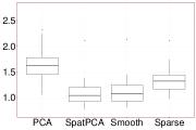
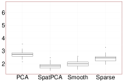
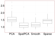
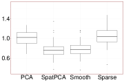
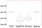
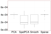
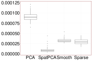
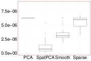
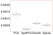
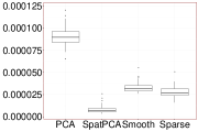
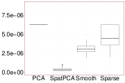
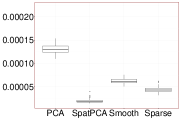
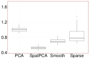
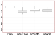
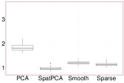
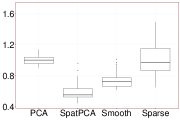
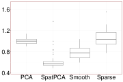
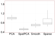
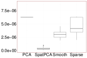
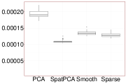
The performance of the four methods in terms of the loss functions (27) and (28) is shown in Figures 3 and 4, respectively, based on 505050 simulation replicates. Once again, SpatPCA outperforms all the other methods in all cases. For (λ1,λ2)=(9,0)subscript𝜆1subscript𝜆290(\lambda_{1},\lambda_{2})=(9,0), the average computation time for SpatPCA (including selection of λ1subscript𝜆1\lambda_{1} and λ2subscript𝜆2\lambda_{2} using 5-fold CV) with K=1,2,5𝐾125K=1,2,5 are 0.0200.0200.020, 0.0650.0650.065 and 0.2640.2640.264 seconds, respectively, which are larger than 0.0020.0020.002 seconds required for PCA. The results were conducted using our R package “SpatPCA” implemented on an iMac PC equipped with a 3.2GHz Intel Core i5 CPU and a 64GB RAM.

(λ1,λ2)=(9,0)subscript𝜆1subscript𝜆290(\lambda_{1},\lambda_{2})=(9,0), K=1𝐾1K=1 (λ1,λ2)=(1,0)subscript𝜆1subscript𝜆210(\lambda_{1},\lambda_{2})=(1,0), K=1𝐾1K=1 (λ1,λ2)=(9,4)subscript𝜆1subscript𝜆294(\lambda_{1},\lambda_{2})=(9,4), K=1𝐾1K=1
Refer to caption Refer to caption Refer to caption
(λ1,λ2)=(9,0)subscript𝜆1subscript𝜆290(\lambda_{1},\lambda_{2})=(9,0), K=2𝐾2K=2 (λ1,λ2)=(1,0)subscript𝜆1subscript𝜆210(\lambda_{1},\lambda_{2})=(1,0), K=2𝐾2K=2 (λ1,λ2)=(9,4)subscript𝜆1subscript𝜆294(\lambda_{1},\lambda_{2})=(9,4), K=2𝐾2K=2
Refer to caption Refer to caption Refer to caption
(λ1,λ2)=(9,0)subscript𝜆1subscript𝜆290(\lambda_{1},\lambda_{2})=(9,0), K=5𝐾5K=5 (λ1,λ2)=(1,0)subscript𝜆1subscript𝜆210(\lambda_{1},\lambda_{2})=(1,0), K=5𝐾5K=5 (λ1,λ2)=(9,4)subscript𝜆1subscript𝜆294(\lambda_{1},\lambda_{2})=(9,4), K=5𝐾5K=5
Refer to caption Refer to caption Refer to caption
(λ1,λ2)=(9,0)subscript𝜆1subscript𝜆290(\lambda_{1},\lambda_{2})=(9,0), K=K^𝐾^𝐾K=\hat{K} (λ1,λ2)=(1,0)subscript𝜆1subscript𝜆210(\lambda_{1},\lambda_{2})=(1,0), K=K^𝐾^𝐾K=\hat{K} (λ1,λ2)=(9,4)subscript𝜆1subscript𝜆294(\lambda_{1},\lambda_{2})=(9,4), K=K^𝐾^𝐾K=\hat{K}
Refer to caption Refer to caption Refer to caption
Figure 3: Boxplots of average squared prediction errors of (27) for various methods in the one-dimensional simulation experiment of Section 4.1 based on 50 simulation replicates.
(λ1,λ2)=(9,0)subscript𝜆1subscript𝜆290(\lambda_{1},\lambda_{2})=(9,0), K=1𝐾1K=1 (λ1,λ2)=(1,0)subscript𝜆1subscript𝜆210(\lambda_{1},\lambda_{2})=(1,0), K=1𝐾1K=1 (λ1,λ2)=(9,4)subscript𝜆1subscript𝜆294(\lambda_{1},\lambda_{2})=(9,4), K=1𝐾1K=1
Refer to caption Refer to caption Refer to caption
(λ1,λ2)=(9,0)subscript𝜆1subscript𝜆290(\lambda_{1},\lambda_{2})=(9,0), K=2𝐾2K=2 (λ1,λ2)=(1,0)subscript𝜆1subscript𝜆210(\lambda_{1},\lambda_{2})=(1,0), K=2𝐾2K=2 (λ1,λ2)=(9,4)subscript𝜆1subscript𝜆294(\lambda_{1},\lambda_{2})=(9,4), K=2𝐾2K=2
Refer to caption Refer to caption Refer to caption
(λ1,λ2)=(9,0)subscript𝜆1subscript𝜆290(\lambda_{1},\lambda_{2})=(9,0), K=5𝐾5K=5 (λ1,λ2)=(1,0)subscript𝜆1subscript𝜆210(\lambda_{1},\lambda_{2})=(1,0), K=5𝐾5K=5 (λ1,λ2)=(9,4)subscript𝜆1subscript𝜆294(\lambda_{1},\lambda_{2})=(9,4), K=5𝐾5K=5
Refer to caption Refer to caption Refer to caption
(λ1,λ2)=(9,0)subscript𝜆1subscript𝜆290(\lambda_{1},\lambda_{2})=(9,0), K=K^𝐾^𝐾K=\hat{K} (λ1,λ2)=(1,0)subscript𝜆1subscript𝜆210(\lambda_{1},\lambda_{2})=(1,0), K=K^𝐾^𝐾K=\hat{K} (λ1,λ2)=(9,4)subscript𝜆1subscript𝜆294(\lambda_{1},\lambda_{2})=(9,4), K=K^𝐾^𝐾K=\hat{K}
Refer to caption Refer to caption Refer to caption
Figure 4: Boxplots of average squared estimation errors of (28) for various methods in the one-dimensional simulation experiment of Section 4.1 based on 50 simulation replicates.

4.2 Two-Dimensional Experiment I

We considered a two-dimensional experiment by generating data according to (3) with K=2𝐾2K=2, 𝝃iN(𝟎,diag(λ1,λ2))similar-tosubscript𝝃𝑖𝑁0diagsubscript𝜆1subscript𝜆2\bm{\xi}_{i}\sim N(\bm{0},\mathrm{diag}(\lambda_{1},\lambda_{2})), ϵiN(𝟎,𝑰)similar-tosubscriptbold-italic-ϵ𝑖𝑁0𝑰\bm{\epsilon}_{i}\sim N(\bm{0},\bm{I}), n=500𝑛500n=500, 𝒔1,,𝒔psubscript𝒔1subscript𝒔𝑝\bm{s}_{1},\dots,\bm{s}_{p} regularly spaced at p=202𝑝superscript202p=20^{2} locations in D=[5,5]2𝐷superscript552D=[-5,5]^{2}. Here ϕ1()subscriptitalic-ϕ1\phi_{1}(\cdot) and ϕ2()subscriptitalic-ϕ2\phi_{2}(\cdot) are given by (29) and (30) with d=2𝑑2d=2 (see the images in the first column of Figure 5).

Estimates of ϕ1()subscriptitalic-ϕ1\phi_{1}(\cdot) based on (λ1,λ2)=(9,0)subscript𝜆1subscript𝜆290(\lambda_{1},\lambda_{2})=(9,0) and K=1𝐾1K=1 Refer to caption Estimates ϕ1()subscriptitalic-ϕ1\phi_{1}(\cdot) based on (λ1,λ2)=(1,0)subscript𝜆1subscript𝜆210(\lambda_{1},\lambda_{2})=(1,0) and K=1𝐾1K=1 Refer to caption Estimates of ϕ1()subscriptitalic-ϕ1\phi_{1}(\cdot) based on (λ1,λ2)=(9,4)subscript𝜆1subscript𝜆294(\lambda_{1},\lambda_{2})=(9,4) and K=2𝐾2K=2 Refer to caption Estimates of ϕ2()subscriptitalic-ϕ2\phi_{2}(\cdot) based on (λ1,λ2)=(9,4)subscript𝜆1subscript𝜆294(\lambda_{1},\lambda_{2})=(9,4) and K=2𝐾2K=2 Refer to caption

Figure 5: Estimates of ϕ1()subscriptitalic-ϕ1\phi_{1}(\cdot) and ϕ2()subscriptitalic-ϕ2\phi_{2}(\cdot) obtained from various methods based on three different combinations of eigenvalues.

We considered three pairs of (λ1,λ2){(9,0),(1,0),(9,4)}subscript𝜆1subscript𝜆2901094(\lambda_{1},\lambda_{2})\in\{(9,0),(1,0),(9,4)\}, and applied the proposed SpatPCA with K{1,2,5}𝐾125K\in\{1,2,5\} and K^^𝐾\hat{K} selected from (17). As in the one-dimensional experiment, we used 5-fold CV of (8) and a two-step procedure to select among the same 11 values of τ1subscript𝜏1\tau_{1} and 313131 values of τ2subscript𝜏2\tau_{2}. Similarly, we used 5-fold CV of (16) to select among the same 11 values of γ𝛾\gamma for covariance function estimation.

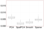
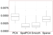
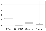
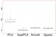
Figure 5 shows the estimates of ϕ1()subscriptitalic-ϕ1\phi_{1}(\cdot) and ϕ2()subscriptitalic-ϕ2\phi_{2}(\cdot) obtained from the four methods for various cases based on a randomly generated dataset. The performance of the four methods in terms of the loss functions (27) and (28) is summarized in Figure 6 and Figure 7, respectively, based on 50 simulation replicates. Similarly to the one-dimensional examples, SpatPCA performs significantly better than all the other methods in all cases. For (λ1,λ2)=(9,0)subscript𝜆1subscript𝜆290(\lambda_{1},\lambda_{2})=(9,0), the average computation time for SpatPCA (including selection of λ1subscript𝜆1\lambda_{1} and λ2subscript𝜆2\lambda_{2} using 5-fold CV) with K=1,2,5𝐾125K=1,2,5 are 3.1053.1053.105, 4.2424.2424.242 and 16.16016.16016.160 seconds, respectively, using the R package “SpatPCA” implemented on an iMac PC with a 3.2GHz Intel Core i5 CPU and a 64GB RAM. While SpatPCA is slower than PCA (requiring only 0.2670.2670.267 seconds), it is reasonably fast and provides much improved results.

(λ1,λ2)=(9,0)subscript𝜆1subscript𝜆290(\lambda_{1},\lambda_{2})=(9,0), K=1𝐾1K=1 (λ1,λ2)=(1,0)subscript𝜆1subscript𝜆210(\lambda_{1},\lambda_{2})=(1,0), K=1𝐾1K=1 (λ1,λ2)=(9,4)subscript𝜆1subscript𝜆294(\lambda_{1},\lambda_{2})=(9,4), K=1𝐾1K=1
Refer to caption Refer to caption Refer to caption
(λ1,λ2)=(9,0)subscript𝜆1subscript𝜆290(\lambda_{1},\lambda_{2})=(9,0), K=2𝐾2K=2 (λ1,λ2)=(1,0)subscript𝜆1subscript𝜆210(\lambda_{1},\lambda_{2})=(1,0), K=2𝐾2K=2 (λ1,λ2)=(9,4)subscript𝜆1subscript𝜆294(\lambda_{1},\lambda_{2})=(9,4), K=2𝐾2K=2
Refer to caption Refer to caption Refer to caption
(λ1,λ2)=(9,0)subscript𝜆1subscript𝜆290(\lambda_{1},\lambda_{2})=(9,0), K=5𝐾5K=5 (λ1,λ2)=(1,0)subscript𝜆1subscript𝜆210(\lambda_{1},\lambda_{2})=(1,0), K=5𝐾5K=5 (λ1,λ2)=(9,4)subscript𝜆1subscript𝜆294(\lambda_{1},\lambda_{2})=(9,4), K=5𝐾5K=5
Refer to caption Refer to caption Refer to caption
(λ1,λ2)=(9,0)subscript𝜆1subscript𝜆290(\lambda_{1},\lambda_{2})=(9,0), K=K^𝐾^𝐾K=\hat{K} (λ1,λ2)=(1,0)subscript𝜆1subscript𝜆210(\lambda_{1},\lambda_{2})=(1,0), K=K^𝐾^𝐾K=\hat{K} (λ1,λ2)=(9,4)subscript𝜆1subscript𝜆294(\lambda_{1},\lambda_{2})=(9,4), K=K^𝐾^𝐾K=\hat{K}
Refer to caption Refer to caption Refer to caption
Figure 6: Boxplots of average squared prediction errors of (27) for various methods in the two-dimensional simulation experiment of Section 4.2 based on 50 simulation replicates.
(λ1,λ2)=(9,0)subscript𝜆1subscript𝜆290(\lambda_{1},\lambda_{2})=(9,0), K=1𝐾1K=1 (λ1,λ2)=(1,0)subscript𝜆1subscript𝜆210(\lambda_{1},\lambda_{2})=(1,0), K=1𝐾1K=1 (λ1,λ2)=(9,4)subscript𝜆1subscript𝜆294(\lambda_{1},\lambda_{2})=(9,4), K=1𝐾1K=1
Refer to caption Refer to caption Refer to caption
(λ1,λ2)=(9,0)subscript𝜆1subscript𝜆290(\lambda_{1},\lambda_{2})=(9,0), K=2𝐾2K=2 (λ1,λ2)=(1,0)subscript𝜆1subscript𝜆210(\lambda_{1},\lambda_{2})=(1,0), K=2𝐾2K=2 (λ1,λ2)=(9,4)subscript𝜆1subscript𝜆294(\lambda_{1},\lambda_{2})=(9,4), K=2𝐾2K=2
Refer to caption Refer to caption Refer to caption
(λ1,λ2)=(9,0)subscript𝜆1subscript𝜆290(\lambda_{1},\lambda_{2})=(9,0), K=5𝐾5K=5 (λ1,λ2)=(1,0)subscript𝜆1subscript𝜆210(\lambda_{1},\lambda_{2})=(1,0), K=5𝐾5K=5 (λ1,λ2)=(9,4)subscript𝜆1subscript𝜆294(\lambda_{1},\lambda_{2})=(9,4), K=5𝐾5K=5
Refer to caption Refer to caption Refer to caption
(λ1,λ2)=(9,0)subscript𝜆1subscript𝜆290(\lambda_{1},\lambda_{2})=(9,0), K=K^𝐾^𝐾K=\hat{K} (λ1,λ2)=(1,0)subscript𝜆1subscript𝜆210(\lambda_{1},\lambda_{2})=(1,0), K=K^𝐾^𝐾K=\hat{K} (λ1,λ2)=(9,4)subscript𝜆1subscript𝜆294(\lambda_{1},\lambda_{2})=(9,4), K=K^𝐾^𝐾K=\hat{K}
Refer to caption Refer to caption Refer to caption
Figure 7: Boxplots of average squared estimation errors of (28) for various methods in the two-dimensional simulation experiment of Section 4.2 based on 50 simulation replicates.

4.3 An Application to a Sea Surface Temperature Dataset

Since the proposed SpatPCA works better when both smoothness and sparseness penalties are involved according to the simulation experiments in Sections 4.1 and 4.2, we applied the proposed SpatPCA with both penalty terms to a sea surface temperature (SST) dataset observed over a region in the Indian Ocean, and only compared it with PCA. The data are monthly averages of SST obtained from the Met Office Marine Data Bank (available at http://www.metoffice.gov.uk/hadobs/hadisst/) on 111 degree latitude by 1 degree longitude (1×1superscript1superscript11^{\circ}\times 1^{\circ}) equiangular grid cells from January 2001 to December 2010 in the region between latitudes 20Nsuperscript20𝑁20^{\circ}N and 20Ssuperscript20𝑆20^{\circ}S and between longitudes 39Esuperscript39𝐸39^{\circ}E and 120Esuperscript120𝐸120^{\circ}E. Out of 40×81=3,2404081324040\times 81=3,240 grid cells, there are 460460460 cells on the land where no data are available. Hence the data we used are observed at p=2,780𝑝2780p=2,780 cells and 120120120 time points. We first detrended the SST data by subtracting the SST for a given cell and a given month by the average SST for that cell and that month over the whole period. We decomposed the data into two parts with one part consisting of 606060 time points of {1,3,,119}13119\{1,3,\dots,119\} for training data, and the other part, consisting of 606060 time points of even numbers, for validation purpose.

We applied SpatPCA on the training data with K𝐾K selected by K^^𝐾\hat{K} of (17)17(\ref{eq:khat}). Similar to the two-step method described in Section 4.1, we selected among 11 values of τ1subscript𝜏1\tau_{1} (including 00, and the other 10 values from 103superscript10310^{3} to 108superscript10810^{8} equally spaced on the log scale) and 31 values of τ2subscript𝜏2\tau_{2} (including 00, and the other 303030 values from 111 to 103superscript10310^{3} equally spaced on the log scale) using 5-fold CV of (8)italic-(8italic-)\eqref{eq:cv}. For both PCA and SpatPCA, we applied 555-fold CV of (16)italic-(16italic-)\eqref{eq:cv.gamma} to select among 11 values of γ𝛾\gamma (including 00 and other 10 values from d^1/103subscript^𝑑1superscript103\hat{d}_{1}/10^{3} to d^1subscript^𝑑1\hat{d}_{1} equally spaced on the log scale), where d^1subscript^𝑑1\hat{d}_{1} is the largest eigenvalue of 𝚽^𝑺𝚽^superscript^𝚽𝑺^𝚽\hat{\bm{\Phi}}^{\prime}\bm{S}\hat{\bm{\Phi}}.

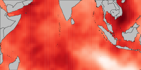
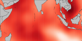
ϕ^1()subscript^italic-ϕ1\hat{\phi}_{1}(\cdot) from PCA                                    ϕ^1()subscript^italic-ϕ1\hat{\phi}_{1}(\cdot) from SpatPCA Refer to caption Refer to caption
Refer to caption
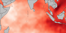
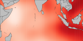
ϕ^2()subscript^italic-ϕ2\hat{\phi}_{2}(\cdot) from PCA                                    ϕ^2()subscript^italic-ϕ2\hat{\phi}_{2}(\cdot) from SpatPCA Refer to caption Refer to caption
Refer to caption

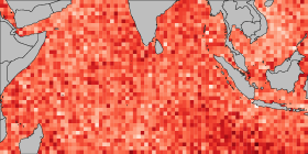
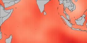
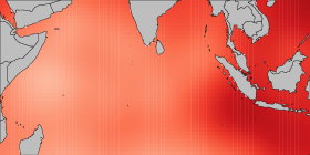
Figure 8: Estimated eigenimages obtained form PCA and SpatPCA over a region in the Indian Ocean, where the gray regions correspond to the land.

The first two dominant patterns estimated from PCA and SpatPCA are shown in Figure 8. Both methods identify similar patterns with the ones estimated from SpatPCA being a bit smoother than those estimated from PCA. The first pattern is a basin-wide mode and the second one corresponds to the east-west dipole mode (Deser et al. (2009)).

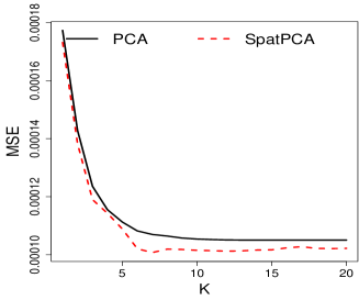
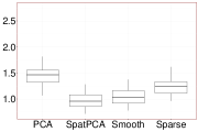
We used the validation data to evaluate the performance between PCA and SpatPCA in terms of the mean squared error (MSE), 𝚺^𝑺vF2/p2superscriptsubscriptnorm^𝚺subscript𝑺𝑣𝐹2superscript𝑝2\|\hat{\bm{\Sigma}}-\bm{S}_{v}\|_{F}^{2}/p^{2}, where 𝚺^^𝚺\hat{\bm{\Sigma}} is a generic estimate of var(𝒀)var𝒀\mathrm{var}(\bm{Y}) based on the training data, and 𝑺vsubscript𝑺𝑣\bm{S}_{v} is the sample covariance matrix based on the validation data. The resulting MSE for PCA is 1.05×1041.05superscript1041.05\times 10^{-4}, which is slightly larger than 1.02×1041.02superscript1041.02\times 10^{-4} for SpatPCA. Figure 9 shows the MSEs with respect to various K𝐾K values for both PCA and SpatPCA. The results indicate that SpatPCA is not sensitive to the choice of K𝐾K as long as K𝐾K is sufficiently large. Our choice of K^=6^𝐾6\hat{K}=6 for SpatPCA based on (17)17(\ref{eq:khat}) appears to be effective, and is smaller than K^=15^𝐾15\hat{K}=15 for PCA.

Refer to caption
Figure 9: Mean squared errors of covariance matrix estimation with respect to K𝐾K for PCA and SpatPCA.

4.4 Two-Dimensional Experiment II

To reflect a real-world situation, we generated data by mimicking the SST dataset analyzed in the previous subsection, except we applied a larger noise variance. Specifically, we generated data according to (3) with K=2𝐾2K=2, 𝝃iN(𝟎,diag(λ1,λ2))similar-tosubscript𝝃𝑖𝑁0diagsubscript𝜆1subscript𝜆2\bm{\xi}_{i}\sim N(\bm{0},\mathrm{diag}(\lambda_{1},\lambda_{2})), ϵiN(𝟎,𝑰)similar-tosubscriptbold-italic-ϵ𝑖𝑁0𝑰\bm{\epsilon}_{i}\sim N(\bm{0},\bm{I}), n=60𝑛60n=60, and at the same 2,78027802,780 locations from the SST dataset. Here ϕ1()subscriptitalic-ϕ1\phi_{1}(\cdot) and ϕ2()subscriptitalic-ϕ2\phi_{2}(\cdot) are given by ϕ^1()subscript^italic-ϕ1\hat{\phi}_{1}(\cdot) and ϕ^2()subscript^italic-ϕ2\hat{\phi}_{2}(\cdot) (see Figure 8) and (λ1,λ2)=(91.3,16.1)subscript𝜆1subscript𝜆291.316.1(\lambda_{1},\lambda_{2})=(91.3,16.1) estimated by SpatPCA in the previous subsection.

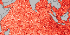
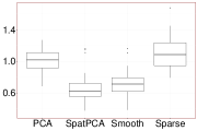
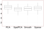
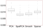
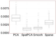
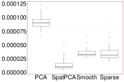
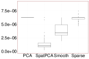
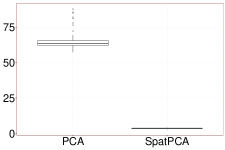
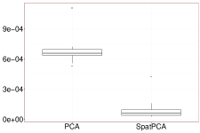
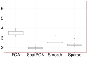
We applied the 5-fold CV of (16) and (17) to select the tuning parameters (τ1,τ2)subscript𝜏1subscript𝜏2(\tau_{1},\tau_{2}) and K𝐾K in the same way as in the previous subsection. Figure 10 shows the estimates of ϕ1()subscriptitalic-ϕ1\phi_{1}(\cdot) and ϕ2()subscriptitalic-ϕ2\phi_{2}(\cdot) for PCA and SpatPCA based on a randomly generated dataset. Because we consider a larger noise variance than those in the previous subsection, the first two patterns estimated from PCA turn out to be very noisy. In contrast, SpatPCA can still reconstruct the first two patterns very well with little noise. The results in terms of the loss functions of (27) and (28) are summarized in Figure 11. Once again, SpatPCA outperforms PCA by a large margin.

ϕ^1()subscript^italic-ϕ1\hat{\phi}_{1}(\cdot) from PCA                                        ϕ^1()subscript^italic-ϕ1\hat{\phi}_{1}(\cdot) from SpatPCA Refer to caption Refer to caption
Refer to caption
ϕ^2()subscript^italic-ϕ2\hat{\phi}_{2}(\cdot) from PCA                                        ϕ^2()subscript^italic-ϕ2\hat{\phi}_{2}(\cdot) from SpatPCA Refer to caption Refer to caption
Refer to caption

Figure 10: Estimates of ϕ1()subscriptitalic-ϕ1\phi_{1}(\cdot) and ϕ2()subscriptitalic-ϕ2\phi_{2}(\cdot) obtained from PCA and SpatPCA in the two-dimensional experiment of Section 4.4 based on a randomly simulated dataset, where the areas in gray are the land.
Refer to caption Refer to caption
(a) (b)
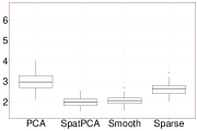
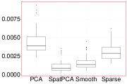
Figure 11: (a) Boxplots of loss function values for PCA and SpatPCA in the two-dimensional simulation experiment of Section 4.4 based on 50 simulation replicates: (a) Average squared prediction errors of (27); (b) Average squared estimation errors of (28).

Acknowledgements

The authors are grateful to the associate editor and the two referees for their insightful and constructive comments, which greatly improve the presentation of this paper. This research was supported in part by ROC Ministry of Science and Technology grant MOST 103-2118-M-001-007-MY3.

Appendix

Proof of Proposition 14.

First, we prove (10). From Corollary 1 of Tzeng and Huang (2015), the minimizer of h(𝚲,σ2)𝚲superscript𝜎2h(\bm{\Lambda},\sigma^{2}) given σ2superscript𝜎2\sigma^{2} is

𝚲^(σ2)=𝑽^diag((d^1σ2γ)+,,(d^Kσ2γ)+)𝑽^.^𝚲superscript𝜎2^𝑽diagsubscriptsubscript^𝑑1superscript𝜎2𝛾subscriptsubscript^𝑑𝐾superscript𝜎2𝛾superscript^𝑽\hat{\bm{\Lambda}}(\sigma^{2})=\hat{\bm{V}}\mathrm{diag}\big{(}(\hat{d}_{1}-\sigma^{2}-\gamma)_{+},\dots,(\hat{d}_{K}-\sigma^{2}-\gamma)_{+}\big{)}\hat{\bm{V}}^{\prime}. (31)

Hence (10) is obtained.

Next, we prove (13). Rewrite the objective function of (9) as:

h(𝚲,σ2)=𝚲superscript𝜎2absent\displaystyle h(\bm{\Lambda},\sigma^{2})= 12𝚽^𝚽^𝑺𝚽^𝚽^𝚽^𝚲𝚽^σ2𝑰pF2+12𝑺𝚽^𝚽^𝑺𝚽^𝚽^F212subscriptsuperscriptnorm^𝚽superscript^𝚽𝑺^𝚽superscript^𝚽^𝚽𝚲superscript^𝚽superscript𝜎2subscript𝑰𝑝2𝐹12subscriptsuperscriptnorm𝑺^𝚽superscript^𝚽𝑺^𝚽superscript^𝚽2𝐹\displaystyle~{}\frac{1}{2}\|\hat{\bm{\Phi}}\hat{\bm{\Phi}}^{\prime}\bm{S}\hat{\bm{\Phi}}\hat{\bm{\Phi}}^{\prime}-\hat{\bm{\Phi}}\bm{\Lambda}\hat{\bm{\Phi}}^{\prime}-\sigma^{2}\bm{I}_{p}\|^{2}_{F}+\frac{1}{2}\|\bm{S}-\hat{\bm{\Phi}}\hat{\bm{\Phi}}^{\prime}\bm{S}\hat{\bm{\Phi}}\hat{\bm{\Phi}}^{\prime}\|^{2}_{F}
+σ2tr(𝚽^𝚽^𝑺𝚽^𝚽^𝑺)+γ𝚽^𝚲𝚽^.superscript𝜎2tr^𝚽superscript^𝚽𝑺^𝚽superscript^𝚽𝑺𝛾subscriptnorm^𝚽𝚲superscript^𝚽\displaystyle~{}+\sigma^{2}\mathrm{tr}(\hat{\bm{\Phi}}\hat{\bm{\Phi}}^{\prime}\bm{S}\hat{\bm{\Phi}}\hat{\bm{\Phi}}^{\prime}-\bm{S})+\gamma\|\hat{\bm{\Phi}}\bm{\Lambda}\hat{\bm{\Phi}}^{\prime}\|_{*}. (32)

From (31) and (32), we have

h(𝚲^(σ2),σ2)=^𝚲superscript𝜎2superscript𝜎2absent\displaystyle h(\hat{\bm{\Lambda}}(\sigma^{2}),\sigma^{2})= 12𝚽^𝚽^𝑺𝚽^𝚽^𝚽^𝚲^(σ2)𝚽^σ2𝑰pF2+γ𝚽^𝚲^(σ2)𝚽^12subscriptsuperscriptnorm^𝚽superscript^𝚽𝑺^𝚽superscript^𝚽^𝚽^𝚲superscript𝜎2superscript^𝚽superscript𝜎2subscript𝑰𝑝2𝐹𝛾subscriptnorm^𝚽^𝚲superscript𝜎2superscript^𝚽\displaystyle~{}\frac{1}{2}\|\hat{\bm{\Phi}}\hat{\bm{\Phi}}^{\prime}\bm{S}\hat{\bm{\Phi}}\hat{\bm{\Phi}}^{\prime}-\hat{\bm{\Phi}}\hat{\bm{\Lambda}}(\sigma^{2})\hat{\bm{\Phi}}^{\prime}-\sigma^{2}\bm{I}_{p}\|^{2}_{F}+\gamma\|\hat{\bm{\Phi}}\hat{\bm{\Lambda}}(\sigma^{2})\hat{\bm{\Phi}}^{\prime}\|_{*}
+12𝑺𝚽^𝚽^𝑺𝚽^𝚽^F2+σ2tr(𝚽^𝚽^𝑺𝚽^𝚽^𝑺)12subscriptsuperscriptnorm𝑺^𝚽superscript^𝚽𝑺^𝚽superscript^𝚽2𝐹superscript𝜎2tr^𝚽superscript^𝚽𝑺^𝚽superscript^𝚽𝑺\displaystyle~{}+\frac{1}{2}\|\bm{S}-\hat{\bm{\Phi}}\hat{\bm{\Phi}}^{\prime}\bm{S}\hat{\bm{\Phi}}\hat{\bm{\Phi}}^{\prime}\|^{2}_{F}+\sigma^{2}\mathrm{tr}(\hat{\bm{\Phi}}\hat{\bm{\Phi}}^{\prime}\bm{S}\hat{\bm{\Phi}}\hat{\bm{\Phi}}^{\prime}-\bm{S})
=\displaystyle= 12k=1K{d^k2(d^kσ2γ)+2}+p2σ4σ2tr(𝑺)+12𝑺𝚽^𝚽^𝑺𝚽^𝚽^F2.12superscriptsubscript𝑘1𝐾superscriptsubscript^𝑑𝑘2superscriptsubscriptsubscript^𝑑𝑘superscript𝜎2𝛾2𝑝2superscript𝜎4superscript𝜎2tr𝑺12subscriptsuperscriptnorm𝑺^𝚽superscript^𝚽𝑺^𝚽superscript^𝚽2𝐹\displaystyle~{}\frac{1}{2}\sum_{k=1}^{K}\big{\{}\hat{d}_{k}^{2}-(\hat{d}_{k}-\sigma^{2}-\gamma)_{+}^{2}\big{\}}+\frac{p}{2}\sigma^{4}-\sigma^{2}\mathrm{tr}(\bm{S})+\frac{1}{2}\|\bm{S}-\hat{\bm{\Phi}}\hat{\bm{\Phi}}^{\prime}\bm{S}\hat{\bm{\Phi}}\hat{\bm{\Phi}}^{\prime}\|^{2}_{F}.

Minimizing h(𝚲^(σ2),σ2)^𝚲superscript𝜎2superscript𝜎2h(\hat{\bm{\Lambda}}(\sigma^{2}),\sigma^{2}), we obtain

σ^2=argminσ20{pσ42σ2tr(𝑺)k=1K(d^kσ2γ)+2}.superscript^𝜎2subscriptsuperscript𝜎20𝑝superscript𝜎42superscript𝜎2tr𝑺superscriptsubscript𝑘1𝐾superscriptsubscriptsubscript^𝑑𝑘superscript𝜎2𝛾2\hat{\sigma}^{2}=\mathop{\arg\min}_{\sigma^{2}\geq 0}\bigg{\{}p\sigma^{4}-2\sigma^{2}\mathrm{tr}(\bm{S})-\sum_{k=1}^{K}(\hat{d}_{k}-\sigma^{2}-\gamma)_{+}^{2}\bigg{\}}. (33)

Clearly, if d^1γsubscript^𝑑1𝛾\hat{d}_{1}\leq\gamma, then σ^2=1ptr(𝑺)superscript^𝜎21𝑝tr𝑺\hat{\sigma}^{2}=\displaystyle\frac{1}{p}\mathrm{tr}(\bm{S}). We remain to consider d^1>γsubscript^𝑑1𝛾\hat{d}_{1}>\gamma. Let

L^=max{L:d^Lγ>σ^2,L=1,,K}.superscript^𝐿:𝐿formulae-sequencesubscript^𝑑𝐿𝛾superscript^𝜎2𝐿1𝐾\hat{L}^{*}=\max\big{\{}L:\hat{d}_{L}-\gamma>\hat{\sigma}^{2},\,L=1,\dots,K\big{\}}.

From (33), σ^2=1pL^(tr(𝑺)k=1L^(d^kγ))superscript^𝜎21𝑝superscript^𝐿tr𝑺superscriptsubscript𝑘1superscript^𝐿subscript^𝑑𝑘𝛾\hat{\sigma}^{2}=\displaystyle\frac{1}{p-\hat{L}^{*}}\bigg{(}\mathrm{tr}(\bm{S})-\sum_{k=1}^{\hat{L}^{*}}(\hat{d}_{k}-\gamma)\bigg{)}. It suffices to show that L^=L^superscript^𝐿^𝐿\hat{L}^{*}=\hat{L}. Since d^L^γ>1pL^(tr(𝑺)k=1L^(d^kγ))subscript^𝑑superscript^𝐿𝛾1𝑝superscript^𝐿tr𝑺superscriptsubscript𝑘1superscript^𝐿subscript^𝑑𝑘𝛾\hat{d}_{\hat{L}^{*}}-\gamma>\displaystyle\frac{1}{p-\hat{L}^{*}}\bigg{(}\mathrm{tr}(\bm{S})-\sum_{k=1}^{\hat{L}^{*}}(\hat{d}_{k}-\gamma)\bigg{)}, by the definition of L^^𝐿\hat{L}, we have L^L^^𝐿superscript^𝐿\hat{L}\geq\hat{L}^{*}, implying d^L^d^L^subscript^𝑑^𝐿subscript^𝑑superscript^𝐿\hat{d}_{\hat{L}}\geq\hat{d}_{\hat{L}^{*}}. Suppose that L^>L^^𝐿superscript^𝐿\hat{L}>\hat{L}^{*}. It immediately follows from the definition of L^superscript^𝐿\hat{L}^{*} that d^L^γσ^2<d^L^γsubscript^𝑑^𝐿𝛾superscript^𝜎2subscript^𝑑superscript^𝐿𝛾\hat{d}_{\hat{L}}-\gamma\leq\hat{\sigma}^{2}<\hat{d}_{\hat{L}^{*}}-\gamma, which contradicts to d^L^d^L^subscript^𝑑^𝐿subscript^𝑑superscript^𝐿\hat{d}_{\hat{L}}\geq\hat{d}_{\hat{L}^{*}}. Therefore, L^=L^^𝐿superscript^𝐿\hat{L}=\hat{L}^{*}. This completes the proof. ∎

References

  • Boyd et al. (2011) {barticle}[author] \bauthor\bsnmBoyd, \bfnmStephen\binitsS., \bauthor\bsnmParikh, \bfnmNeal\binitsN., \bauthor\bsnmChu, \bfnmEric\binitsE., \bauthor\bsnmPeleato, \bfnmBorja\binitsB. and \bauthor\bsnmEckstein, \bfnmJonathan\binitsJ. (\byear2011). \btitleDistributed optimization and statistical learning via the alternating direction method of multipliers. \bjournalFoundations and Trends in Machine Learning \bvolume3 \bpages1-124. \endbibitem
  • Cressie and Johannesson (2008) {barticle}[author] \bauthor\bsnmCressie, \bfnmNoel\binitsN. and \bauthor\bsnmJohannesson, \bfnmGardar\binitsG. (\byear2008). \btitleFixed Rank Kriging for Very Large Spatial Data Sets. \bjournalJournal of the Royal Statistical Society. Series B \bvolume70 \bpages209-226. \endbibitem
  • d’Aspremont, Bach and Ghaoui (2008) {barticle}[author] \bauthor\bsnmd’Aspremont, \bfnmAlexandre\binitsA., \bauthor\bsnmBach, \bfnmFrancis\binitsF. and \bauthor\bsnmGhaoui, \bfnmLaurent El\binitsL. E. (\byear2008). \btitleOptimal solutions for sparse principal component analysis. \bjournalJournal of Machine Learning Research \bvolume9 \bpages1269-1294. \endbibitem
  • Demsar et al. (2013) {barticle}[author] \bauthor\bsnmDemsar, \bfnmUrska\binitsU., \bauthor\bsnmHarris, \bfnmPaul\binitsP., \bauthor\bsnmBrunsdon, \bfnmChris\binitsC., \bauthor\bsnmFotheringham, \bfnmA. Stewart\binitsA. S. and \bauthor\bsnmMcLoone, \bfnmSean\binitsS. (\byear2013). \btitlePrincipal component analysis on spatial data: an overview. \bjournalAnnals of the Association of American Geographers \bvolume103 \bpages106-128. \endbibitem
  • Deser et al. (2009) {barticle}[author] \bauthor\bsnmDeser, \bfnmClara\binitsC., \bauthor\bsnmAlexander, \bfnmMichael A.\binitsM. A., \bauthor\bsnmXie, \bfnmShang-Ping\binitsS.-P. and \bauthor\bsnmPhillips, \bfnmAdam S.\binitsA. S. (\byear2009). \btitleSea surface temperature variability: patterns and mechanisms. \bjournalAnnual Review of Marine Science \bvolume2 \bpages115-143. \endbibitem
  • Friedman, Hastie and Tibshirani (2010) {barticle}[author] \bauthor\bsnmFriedman, \bfnmJerome\binitsJ., \bauthor\bsnmHastie, \bfnmTrevor\binitsT. and \bauthor\bsnmTibshirani, \bfnmRobert\binitsR. (\byear2010). \btitleRegularization paths for generalized linear models via coordinate descent. \bjournalJournal of Statistical Software \bvolume33 \bpages1-22. \endbibitem
  • Gabay and Mercier (1976) {barticle}[author] \bauthor\bsnmGabay, \bfnmDaniel\binitsD. and \bauthor\bsnmMercier, \bfnmBertrand\binitsB. (\byear1976). \btitleA dual algorithm for the solution of nonlinear variational problems via finite element approximation. \bjournalComputer and Mathematics with Applications \bvolume2 \bpages17-40. \endbibitem
  • Green and Silverman (1994) {bbook}[author] \bauthor\bsnmGreen, \bfnmP. J.\binitsP. J. and \bauthor\bsnmSilverman, \bfnmB. W.\binitsB. W. (\byear1994). \btitleNonparametric regression and generalized linear model: a roughness penalty approach. \bpublisherChapman and Hall. \endbibitem
  • Guo et al. (2010) {barticle}[author] \bauthor\bsnmGuo, \bfnmJian\binitsJ., \bauthor\bsnmJames., \bfnmGareth\binitsG., \bauthor\bsnmLevina, \bfnmElizaveta\binitsE., \bauthor\bsnmMichailidis, \bfnmGeorge\binitsG. and \bauthor\bsnmZhu, \bfnmJi\binitsJ. (\byear2010). \btitlePrincipal component analysis with sparse fused loadings. \bjournalJournal of Computational and Graphical Statistics \bvolume19 \bpages930-946. \endbibitem
  • Hannachi, Jolliffe and Stephenson (2007) {barticle}[author] \bauthor\bsnmHannachi, \bfnmA.\binitsA., \bauthor\bsnmJolliffe, \bfnmIan T.\binitsI. T. and \bauthor\bsnmStephenson, \bfnmD. B.\binitsD. B. (\byear2007). \btitleEmpirical orthogonal functions and related techniques in atmospheric science: A review. \bjournalInternational Journal of Climatology \bvolume27 \bpages1119-1152. \endbibitem
  • Hong and Lian (2013) {barticle}[author] \bauthor\bsnmHong, \bfnmZhaoping\binitsZ. and \bauthor\bsnmLian, \bfnmHeng\binitsH. (\byear2013). \btitleSparse-smooth regularized singular value decomposition. \bjournalJournal of Multivariate Analysis \bvolume117 \bpages163-174. \endbibitem
  • Huang, Shen and Buja (2008) {barticle}[author] \bauthor\bsnmHuang, \bfnmJianhua Z.\binitsJ. Z., \bauthor\bsnmShen, \bfnmHaipeng\binitsH. and \bauthor\bsnmBuja, \bfnmAndreas\binitsA. (\byear2008). \btitleFunctional principal components analysis via penalized rank one approximation. \bjournalElectronic Journal of Statistics \bvolume2 \bpages678-695. \endbibitem
  • Jolliffe (1987) {barticle}[author] \bauthor\bsnmJolliffe, \bfnmIan T.\binitsI. T. (\byear1987). \btitleRotation of principal components: Some comments. \bjournalJournal of Climatology \bvolume7 \bpages507–510. \endbibitem
  • Jolliffe (2002) {bbook}[author] \bauthor\bsnmJolliffe, \bfnmIan T.\binitsI. T. (\byear2002). \btitlePrincipal component analysis. \bpublisherWiley Online Library. \endbibitem
  • Jolliffe, Uddin and Vines (2002) {barticle}[author] \bauthor\bsnmJolliffe, \bfnmIan T.\binitsI. T., \bauthor\bsnmUddin, \bfnmMudassir\binitsM. and \bauthor\bsnmVines, \bfnmS. K.\binitsS. K. (\byear2002). \btitleSimplified EOFs–three alternatives to rotation. \bjournalClimate Research \bvolume20 \bpages271-279. \endbibitem
  • Kang and Cressie (2011) {barticle}[author] \bauthor\bsnmKang, \bfnmEmily L.\binitsE. L. and \bauthor\bsnmCressie, \bfnmNoel\binitsN. (\byear2011). \btitleBayesian Inference for the Spatial Random Effects Model. \bjournalJournal of the American Statistical Association \bvolume106 \bpages972-983. \endbibitem
  • Karhunen (1947) {barticle}[author] \bauthor\bsnmKarhunen, \bfnmKari\binitsK. (\byear1947). \btitleÜber lineare methoden in der Wahrscheinlichkeitsrechnung. \bjournalAnnales Academiæ Scientiarum Fennicæ Series A \bvolume37 \bpages1-79. \endbibitem
  • Loève (1978) {bbook}[author] \bauthor\bsnmLoève, \bfnmMichel\binitsM. (\byear1978). \btitleProbability theory. \bpublisherSpringer-Verlag, New York. \endbibitem
  • Lu and Zhang (2012) {barticle}[author] \bauthor\bsnmLu, \bfnmZhaosong\binitsZ. and \bauthor\bsnmZhang, \bfnmYong\binitsY. (\byear2012). \btitleAn augmented Lagrangian approach for sparse principal component analysis. \bjournalMathematical Programming \bvolume135 \bpages149–193. \endbibitem
  • Ramsay and Silverman (2005) {bbook}[author] \bauthor\bsnmRamsay, \bfnmJ. O.\binitsJ. O. and \bauthor\bsnmSilverman, \bfnmB. W.\binitsB. W. (\byear2005). \btitleFunctional data analysis, \bedition2nd ed. \bpublisherNew York: Springer. \endbibitem
  • Richman (1986) {barticle}[author] \bauthor\bsnmRichman, \bfnmMichael B.\binitsM. B. (\byear1986). \btitleRotation of principal components. \bjournalJournal of Climatology \bvolume6 \bpages293-335. \endbibitem
  • Richman (1987) {barticle}[author] \bauthor\bsnmRichman, \bfnmMichael B.\binitsM. B. (\byear1987). \btitleRotation of principal components: A reply. \bjournalJournal of Climatology \bvolume7 \bpages511–520. \endbibitem
  • Shen and Huang (2008) {barticle}[author] \bauthor\bsnmShen, \bfnmHaipeng\binitsH. and \bauthor\bsnmHuang, \bfnmJianhua Z.\binitsJ. Z. (\byear2008). \btitleSparse principal component analysis via regularized low rank matrix approximation. \bjournalJournal of Multivariate Analysis \bvolume99 \bpages1015-1034. \endbibitem
  • Tibshirani (1996) {barticle}[author] \bauthor\bsnmTibshirani, \bfnmRobert\binitsR. (\byear1996). \btitleRegression shrinkage and selection via the Lasso. \bjournalJournal of the Royal Statistical Society. Series B \bvolume58 \bpages267-288. \endbibitem
  • Tzeng and Huang (2015) {barticle}[author] \bauthor\bsnmTzeng, \bfnmShengLi\binitsS. and \bauthor\bsnmHuang, \bfnmHsin-Cheng\binitsH.-C. (\byear2015). \btitleNon-stationary multivariate spatial covariance estimation via low-rank regularization. \bjournalStatistical Sinica \bvolume26 \bpages151-172. \endbibitem
  • Yao, Muller and Wang (2005) {barticle}[author] \bauthor\bsnmYao, \bfnmFang\binitsF., \bauthor\bsnmMuller, \bfnmHans-Georg\binitsH.-G. and \bauthor\bsnmWang, \bfnmJane-Ling\binitsJ.-L. (\byear2005). \btitleFunctional data analysis for sparse longitudinal data. \bjournalJournal of the American Statistical Association \bvolume100 \bpages577-590. \endbibitem
  • Zou, Hastie and Tibshirani (2006) {barticle}[author] \bauthor\bsnmZou, \bfnmHui\binitsH., \bauthor\bsnmHastie, \bfnmTrevor\binitsT. and \bauthor\bsnmTibshirani, \bfnmRobert\binitsR. (\byear2006). \btitleSparse principal component analysis. \bjournalJournal of Computational and Graphical Statistics \bvolume15 \bpages265-286. \endbibitem