Constraint-based sequence mining
using constraint programming

Abstract

The goal of constraint-based sequence mining is to find sequences of symbols that are included in a large number of input sequences and that satisfy some constraints specified by the user. Many constraints have been proposed in the literature, but a general framework is still missing. We investigate the use of constraint programming as general framework for this task.

We first identify four categories of constraints that are applicable to sequence mining. We then propose two constraint programming formulations. The first formulation introduces a new global constraint called exists-embedding. This formulation is the most efficient but does not support one type of constraint. To support such constraints, we develop a second formulation that is more general but incurs more overhead. Both formulations can use the projected database technique used in specialised algorithms.

Experiments demonstrate the flexibility towards constraint-based settings and compare the approach to existing methods.

1 Introduction

In AI in general and in data mining in particular, there is an increasing interest in developing general methods for data analysis. In order to be useful, such methods should be easy to extend with domain-specific knowledge.

In pattern mining, the frequent sequence mining problem has already been studied in depth, but usually with a focus on efficiency and less on generality and extensibility. An important step in the development of more general approaches was the cSpade algorithm [19] which supports a variety constraints. It supports many constraints such as constraints on the length of the pattern, on the maximum gap in embeddings or on the discriminative power of the patterns between datasets. Many other constraints have been integrated into specific mining algorithms (e.g. [6, 17, 16, 13]). However, none of these are truly generic in that adding extra constraints usually amounts to changing the data-structures used in the core of the algorithm.

For itemset mining, the simplest form of pattern mining, it has been shown that constraint programming (CP) can be used as a generic framework for constraint-based mining [5] and beyond [14, 11]. Recent works have also investigated the usage of CP-based approaches for mining sequences with explicit wildcards [3, 7, 8]. A wildcard represents the presence of exactly one arbitrary symbol in that position in the sequence.

The main difference between mining itemsets, sequences with wildcards and standard sequences lies in the complexity of testing whether a pattern is included in another itemset/sequence, e.g. from the database. For itemsets, this is simply testing the subset inclusion relation which is easy to encode in CP. For sequences with wildcards and general sequences, one has to check whether an embedding exists (matching of the individual symbols). But in case only few embeddings are possible, as in sequences with explicit wildcards, this can be done with a disjunctive constraint over all possible embeddings [8]. In general sequence (the setting we address in this paper), a pattern of size $m$ can be embedded into a sequence of size $n$ in $O(n^{m})$ different ways, hence prohibiting a direct encoding or enumeration.

The contributions of this paper are as follows:

• We present four categories of user-constraints, this categorization will be useful to compare the generality of the two proposed models.

• We introduce an exists-embedding global constraint for sequences, and show the relation to projected databases and projected frequency used in the sequence mining literature to speedup the mining process [6, 20].

• We propose a more general formulation using a decomposition of the exists-embedding constraint. Searching whether an embedding exists for each transaction is not easily expressed in CP and requires a modified search procedure.

• We investigating the effect of adding constraints, and compare our method with state-of-the-art sequence mining algorithms.

The rest of the paper is organized as follows: Section 2 formally introduces the sequence mining problem and the constraint categories. Section 3 explains the basics of encoding sequence mining in CP. Section 4 and 5 present the model with the global constraint and the decomposition respectively. Section 6 presents the experiments. After an overview of related work (Section 7), we discuss the proposed approach and results in Section 8.

2 Sequence mining

Sequence mining [1] can be seen as a variation of the well-known itemset mining problem proposed in [2]. In itemset mining, one is given a set of transactions, where each transaction is a set of items, and the goal is to find patterns (i.e. sets of items) that are included in a large number of transactions. In sequence mining, the problem is similar except that both transactions and patterns are ordered, (i.e. they are sequences instead of sets) and symbols can be repeated. For example, ${\mathrm{\langle{\mathrm{b,a,c,b}}\rangle}}$ and ${\mathrm{\langle{\mathrm{a,c,c,b,b}}\rangle}}$ are two sequences, and the sequence ${\mathrm{\langle{\mathrm{a,b}}\rangle}}$ is one possible pattern included in both.

This problem is known in the literature under multiple names, such as embedded subsequence mining, sequential pattern mining, flexible motif mining, or serial episode mining depending on the application.

2.1 Frequent sequence mining: problem statement

A key concept of any pattern mining setting is the pattern inclusion relation. In sequence mining, a pattern is included in a transaction if there exists an embedding of that sequence in the transaction; where an embedding is a mapping of every symbol in the pattern to the same symbol in the transaction such that the order is respected.

Definition 1 (Embedding in a sequence)

Let $S=\langle s_{1},\ldots,s_{m}\rangle$ and $S^{\prime}=\langle s^{\prime}_{1},\ldots,s^{\prime}_{n}\rangle$ be two sequences of size $m$ and $n$ respectively with $m\leq n$. The tuple of integers $e=(e_{1},\ldots,e_{m})$ is an embedding of $S$ in $S^{\prime}$ (denoted $S\sqsubseteq_{e}S^{\prime}$) if and only if:

$$S\sqsubseteq_{e}S^{\prime}\leftrightarrow e_{1}<\ldots<e_{m}~{}\mbox{and}~{}\forall i\in 1,\ldots,m:s_{i}=s^{\prime}_{e_{i}}$$ (1)

For example, let $S={\mathrm{\langle{\mathrm{a,b}}\rangle}}$ be a pattern, then $(2,4)$ is an embedding of $S$ in ${\mathrm{\langle{\mathrm{b,a,c,b}}\rangle}}$ and $(1,4),(1,5)$ are both embeddings of $S$ in ${\mathrm{\langle{\mathrm{a,c,c,b,b}}\rangle}}$. An alternative setting considers sequences of itemsets instead of sequences of individual symbols. In this case, the definition is $S\sqsubseteq_{e}S^{\prime}\leftrightarrow e_{1}<\ldots<e_{n}~{}\mbox{and}~{}\forall i\in 1,\ldots,n:s_{i}\subseteq s^{\prime}_{e_{i}}$. We do not consider this setting further in this paper, though it is an obvious extension.

We can now define the sequence inclusion relation as follows:

Definition 2 (Inclusion relation for sequences)

Given two sequences $S$ and $S^{\prime}$, $S$ is included in $S^{\prime}$ (denoted $S\sqsubseteq S^{\prime}$) if there exists an embedding $e$ of $S$ in $S^{\prime}$:

$$S\sqsubseteq S^{\prime}\leftrightarrow\exists e~{}\mbox{s.t.}~{}S\sqsubseteq_{e}S^{\prime}.$$ (2)

To continue on the example above, $S={\mathrm{\langle{\mathrm{a,b}}\rangle}}$ is included in both ${\mathrm{\langle{\mathrm{b,a,c,b}}\rangle}}$ and ${\mathrm{\langle{\mathrm{a,c,c,b,b}}\rangle}}$ but not in ${\mathrm{\langle{\mathrm{c,b,a,a}}\rangle}}$.

Definition 3 (Sequential dataset)

Given an alphabet of symbols $\Sigma$, a sequential dataset $D$ is a multiset of sequences defined over symbols in $\Sigma$.

Each sequence in $D$ is called a transaction using the terminology from itemset mining. The number of transactions in $D$ is denoted $|D|$ and the sum of the lengths of every transaction in $D$ is denoted $||D||$ ($||D||=\sum_{i=1}^{|D|}|T_{i}|$). Furthermore, we use dataset as a shorthand for sequential dataset when it is clear from context.

Given a dataset $D=\{T_{i},\ldots,T_{n}\}$, one can compute the cover of a sequence $S$ as the set of all transactions $T_{i}$ that contain $S$:

$$cover(S,D)=\{T_{i}\in D:S\sqsubseteq T_{i}\}$$ (3)

We can now define frequent sequence mining, where the goal is to find all patterns that are frequent in the database; namely, the size of their cover is sufficiently large.

Definition 4 (Frequent sequence mining)

Given:

1. an alphabet $\Sigma$

2. a sequential dataset $D=\{T_{1},\ldots,T_{n}\}$ defined over $\Sigma$

3. a minimum frequency threshold $\theta$,

enumerate all sequences $S$ such that $|cover(S,D)|\geq\theta$.

In large datasets, the number of frequent sequences is often too large to be analyzed by a human. Extra constraints can be added to extract fewer, but more relevant or interesting patterns. Many such constraints have been studied in the past.

2.2 Constraints

Constraints typically capture background knowledge and are provided by the user. We identify four categories of constraints for sequence mining: 1) constraints over the pattern, 2) constraints over the cover set, 3) constraints over the inclusion relation and 4) preferences over the solution set.

2.2.1 Constraints on the pattern

These put restrictions on the structure of the pattern. Typical examples include size constraints or regular expression constraints.
Size constraints: A size constraint is simply $|S|\gtrless\alpha$ where $\gtrless\in\{=,\neq,>,\geq,<,\leq\}$ and $\alpha$ is a user-supplied threshold. It is used to discard small patterns.
Item constraints: One can constrain a symbol $t$ to surely be in the pattern: $\exists s\in S:s=t$; or that it can not appear in the pattern: $\forall s\in S:s\neq t$, or more complex logical expressions over the symbols in the pattern.
Regular expression constraints: Let $R$ be a regular expression over the vocabulary $V$ and $L_{R}$ be the language of sequences recognised by $R$, then for any sequence pattern $S$ over $V$, the $match\mbox{-}regular$ constraint requires that $S\in L_{R}$ [6].

2.2.2 Constraints on the cover set.

The minimum frequency constraint $|cover(S,D)|\geq\theta$ is the most common example of a constraint over the cover set. Alternatively, one can impose the maximum frequency constraint: $|cover(S,D)|\leq\beta$
Discriminating constraints: In case of multiple datasets, discriminating constraints require that patterns effectively distinguish the datasets from each other. Given two datasets $D_{1}$ and $D_{2}$, one can require that the ratio between the size of the cover of both is above a threshold: $\frac{|cover(S,D_{1})|}{|cover(S,D_{2})|}\geq\alpha$. Other examples include more statistical measures such as information gain and entropy [12].

2.2.3 Constraints over the inclusion relation.

The inclusion relation in definition 2 states that $S\sqsubseteq S^{\prime}\leftrightarrow\exists e~{}\mbox{s.t.}~{}S\sqsubseteq_{e}S^{\prime}$. Hence, an embedding of a pattern can match symbols that are far apart in the transaction. For example, the sequence ${\mathrm{\langle{\mathrm{a,c}}\rangle}}$ is embedded in the transaction ${\mathrm{\langle{\mathrm{a,b,b,b,\ldots,b,c}}\rangle}}$ independently of the distance between ${\mathrm{a}}$ and ${\mathrm{c}}$ in the transaction. This is undesirable when mining datasets with long transactions. The $max\mbox{-}gap$ and $max\mbox{-}span$ constraints [19] impose a restriction on the embedding, and hence on the inclusion relation. The $max\mbox{-}gap$ constraint is satisfied on a transaction $T_{i}$ if an embedding $e$ maps every two consecutive symbols in $S$ to symbols in $T_{i}$ that are close to each-other: $max\mbox{-}gap_{i}(e)\Leftrightarrow\forall{j\in 2..|T_{i}|},(e_{j}-e_{j-1}-1)\leq\gamma$. For example, the sequence ${\mathrm{\langle{\mathrm{abc}}\rangle}}$ is embedded in the transaction $\mathrm{\langle{\mathrm{adddbc}}\rangle}$ with a maximum gap of 3 whereas $\mathrm{\langle{\mathrm{ac}}\rangle}$ is not. The $max\mbox{-}span$ constraint requires that the distance between the first and last position of the embedding of all transactions $T_{i}$ is below a threshold $\gamma$: $max\mbox{-}span_{i}(e)\Leftrightarrow e_{|T_{i}|}-e_{1}+1\leq\gamma$.

2.2.4 Preferences over the solution set.

A pairwise preference over the solution set expresses that a pattern $A$ is preferred over a pattern $B$. In [11] it was shown that condensed representations like closed, maximal and free patterns can be expressed as pairwise preference relations. Skypatterns [14] and multi-objective optimisation can also be seen as preference over patterns. As an example, let $\Delta$ be the set of all patterns; then, the set of all closed patterns is $\{S\in\Delta|\nexists S^{\prime}\mbox{ s.t. }S\sqsubset S^{\prime}\mbox{ and }cover(S,D)=cover(S^{\prime},D)\}$.

3 Sequence Mining in Constraint Programming

In constraint programming, problems are expressed as a constraint satisfaction problem (CSP), or a constraint optimisation problem (COP). A CSP $X=(V,D,C)$ consists of a set of variables $V$, a finite domain $D$ that defines for each variable $v\in V$ the possible values that it can take, and a set of constraints $C$ over the variables in $V$. A solution to a CSP is an assignment of each variable to a value from its domain such that all constraints are satisfied. A COP additionally consists of an optimisation criterion $f(V)$ that expresses the quality of the solution.

There is no restriction on what a constraint $C$ can represent. Examples include logical constraints like ${\bf X}\wedge{\bf Y}$ or ${\bf X}\rightarrow{\bf Y}$ and mathematical constraints such as ${\bf Z}={\bf X}+{\bf Y}$ etc. Each constraint has a corresponding propagator that ensures the constraint is satisfied during the search. Many global constraints have been proposed, such as alldifferent, which have a custom propagator that is often more efficient then if one would decompose that constraint in terms of simple logical or mathematical constraints. A final important concept used in this paper is that of reified constraints. A reified constraint is of the form ${\bf B}\leftrightarrow C^{\prime}$ where ${\bf B}$ is a Boolean variable which will be assigned to the truth value of constraint $C^{\prime}$. Reified constraints have their own propagator too.

Variables and domains for modeling sequence mining.

Modeling a problem as a CSP requires the definition of a set of variables with a finite domain, and a set of constraints. One solution to the CSP will correspond to one pattern, that is, one frequent sequence.

We model the problem using an array ${\bf S}$ of integer variables representing the characters of the sequence and an array ${\bf C}$ of Boolean variables representing which transactions include the pattern. This is illustrated in Fig. 1:

Figure 1: Example assignment; blue boxes represent variables, white boxes represent data.

1. $T_{1}$ and $T_{2}$ represent two transactions given as input. We denote the number of transactions by $n$;

2. The array of variables ${\bf S}$ represents the sequence pattern. Each variable ${\bf S_{j}}$ represents the character in the $j$th position of the sequence. The size of ${\bf S}$ is determined by the length of the longest transactions (in the example this is $4$). We want to allow patterns that have fewer than $max_{i}(|T_{i})$ characters, hence we use $\epsilon$ to represent an unused position in ${\bf S}$. The domain of each variable ${\bf S_{j}}$ is thus $\Sigma\cup\{\epsilon\}$;

3. Boolean variables ${\bf C_{i}}$ represent whether the pattern is included in transaction $T_{i}$, that is, whether ${\bf S}\sqsubseteq T_{i}$. In the example, this is the case for $T_{1}$ but not for $T_{2}$.

What remains to be defined is the constraints. The key part here is how to model the inclusion relation; that is, the constraint that verifies whether a pattern is included in the transaction. Conceptually, this is the following reified constraint: ${\bf C_{i}}\leftrightarrow\exists e~{}\mbox{s.t.}~{}{\bf S}\sqsubseteq_{e}T_{i}$. As mentioned in the introduction, the number of possible embeddings is exponential in the size of the pattern. Hence, one can not model this as a disjunctive constraint over all possible embeddings (as is done for sequences with explicit wildcards [8]).

We propose two approaches to cope with this problem: one with a global constraint that verifies the inclusion relation directly on the data, and one in which the inclusion relation is decomposed and the embedding is exposed through variables.

4 Sequence mining with a global exists-embedding constraint

The model consists of three parts: encoding of the pattern, of the minimum frequency constraint and finally of the inclusion relation using a global constraint.

Variable-length pattern:

The array ${\bf S}$ has length $k$; patterns with $l<k$ symbols are represented with $l$ symbols from $\Sigma$ and $(k-l)$ times an $\epsilon$ value. To avoid enumerating the same pattern with $\epsilon$ values in different positions, $\epsilon$ values can only appear at the end:

$$\begin{gathered}\forall j\in 1..(k-1):{\bf S_{j}}=\epsilon\rightarrow{\bf S_{j+1}}=\epsilon\end{gathered}$$ (4)

Minimum frequency:

At least $\theta$ transactions should include the pattern. This inclusion is indicated by the array of Boolean variables ${\bf C}$:

$$\begin{gathered}\sum_{i=1}^{n}{\bf C_{i}}\geq\theta\end{gathered}$$ (5)

Global exists-embedding constraint:

The goal is to encode the relation: ${\bf C_{i}}\leftrightarrow\exists e~{}\mbox{s.t.}~{}{\bf S}\sqsubseteq_{e}T_{i}.$

Algorithm 1 Incremental propagator for ${\bf C_{i}}\leftrightarrow\exists e~{}\mbox{s.t.}~{}{\bf S}\sqsubseteq_{e}T_{i}$:

internal state, $pos_{S}$: current position in ${\bf S}$ to check, initially 1
internal state, $pos_{e}$: current position in $T_{i}$ to match to, initially 1

1:while $pos_{S}\leq|T_{i}|$ and ${\bf S}$[$pos_{S}$] is assigned do $\triangleright$ note that $|T_{i}|\leq|{\bf S}|$

2:    if ${\bf S}$[$pos_{S}$] $\neq\epsilon$ then

3:        while not ($T_{i}[pos_{e}]={\bf S}[pos_{S}])$ and $pos_{e}\leq|T_{i}|$ do $\triangleright$ find match

4:           $pos_{e}\leftarrow pos_{e}+1$

5:        end while

6:        if $pos_{e}\leq|T_{i}|$ then $\triangleright$ match found, on to next one

7:           $pos_{S}\leftarrow pos_{S}+1$; $pos_{e}\leftarrow pos_{e}+1$

8:        else

9:           propagate ${\bf C_{i}}=False$ and return         

10:    else$\triangleright$ previous ones matched and rest is $\epsilon$

11:        propagate ${\bf C_{i}}=True$ and return     

12:end while

13:if $pos_{S}>|{\bf S}|$ then $\triangleright$ previous ones matched and reached end of sequence

14:    propagate ${\bf C_{i}}=True$ and return

15:if $pos_{S}>|T_{i}|$ and $|T_{i}|<|{\bf S}|$ then

16:    let $R\leftarrow{\bf S}[|T_{i}|+1]$

17:    if $R$ is assigned and $R=\epsilon$ then $\triangleright$ S should not be longer than this transaction

18:        propagate ${\bf C_{i}}=True$ and return     

19:    if $\epsilon$ is not in the domain of $R$ then

20:        propagate ${\bf C_{i}}=False$ and return     

21:if ${\bf C_{i}}$ is assigned and ${\bf C_{i}}=True$ then

22:    propagate by removing from ${\bf S}[pos_{S}]$ all symbols not in $\langle T_{i}[pos_{e}]..T_{i}[|T_{i}|]\rangle$ except $\epsilon$

The propagator algorithm for this constraint is given in Algorithm 1. It is an incremental propagator that should be run when one of the ${\bf S}$ variables is assigned. Line 1 will loop over the variables in ${\bf S}$ until reaching an unassigned one at position $pos_{S}$. In the sequence mining literature, the sequence $\langle{\bf S_{1}}..{\bf S_{{pos_{S}}}}\rangle$ is called the prefix. For each assigned ${\bf S_{j}}$ variable, a matching element in the transaction is sought, starting from the position $pos_{e}$ after the element that matched the previous ${\bf S_{j-1}}$ assigned variable. If no such match is found then an embedding can not be found and ${\bf C_{i}}$ is set to false.

Line 11 is called when an ${\bf S_{j}}$ variable is assigned to $\epsilon$. This line can only be reached if all previous values of ${\bf S}$ are assigned and were matched in $T_{i}$, hence the propagator can set ${\bf C_{i}}$ to true and quit. Similarly for line 14 when the end of the sequence is reached, and lines 15-20 in case the transaction is smaller than the sequence. Lines 21-22 propagate the remaining possible symbols from $T_{i}$ to the first unassigned ${\bf S}$ variable in case ${\bf C_{i}}=True$.

The propagator algorithm has complexity $O(|T_{i}|)$: the loop on line 1 is run up to $|T_{i}|$ times and on line 3 at most $|T_{i}|$ times in total, as $pos_{e}$ is monotonically increasing.

4.1 Improved pruning with projected frequency

Compared to specialised sequence mining algorithms, $pos_{S}$ in Algorithm 1 points to the first position in ${\bf S}$ after the current prefix. Dually, $pos_{e}$ points to the position after the first match of the prefix in the transaction. If one would project the prefix away, only the symbols in the transaction from $pos_{e}$ on would remain; this is known as prefix projection [6]. Given prefix ${\mathrm{\langle{\mathrm{a,c}}\rangle}}$ and transaction ${\mathrm{\langle{\mathrm{b,a,a,e,c,b,c,b,b}}\rangle}}$ the projected transaction is ${\mathrm{\langle{\mathrm{b,c,b,b}}\rangle}}$.

The concept of a prefix-projected database can be used to recompute the frequency of all symbols in the projected database. If a symbol is present but not frequent in the projected database, one can avoid searching over it. This is known to speed up specialised mining algorithms considerably [6, 16].

To achieve this in the above model, we need to adapt the global propagator so that it exports the symbols that still appear after $pos_{e}$. We introduce an auxiliary integer variable ${\bf X_{i}}$ for every transaction $T_{i}$, whose domain represents these symbols (the set of symbols is monotonically decreasing). To avoid searching over infrequent symbols, we define a custom search routine (brancher) over the ${\bf S}$ variables. It first computes the local frequencies of all symbols based on the domains of the ${\bf X_{i}}$ variables; symbols that are locally infrequent will not not be branched over. See Appendix 0.A for more details.

4.2 Constraints

This formulation supports a variety of constraints, namely on the pattern (type 1), on the cover set (type 2) and over the solution set (type 4). For example, the type 1 constraint $min\mbox{-}size$, constrains the size of the pattern to be larger than a user-defined threshold $\alpha$. This constraint can be formalised as follows.

$$\begin{gathered}\sum_{j=1}^{k}\bf\left[S_{j}\neq\epsilon\right]\geq\alpha\end{gathered}$$ (6)

Minimum frequency in Equation (5) is an example of a constraint of type 2, over the cover set. Another example is the discriminative constraint mentioned in Section 2.2: given two datasets $D_{1}$ and $D_{2}$, one can require that the ratio between the cover in the two datasets is larger than a user defined threshold $\alpha$: $\frac{|cover(S,D_{1})|}{|cover(S,D_{2})|}\geq\alpha$. Let $D=D_{1}\cup D_{2}$ and let $t_{1}=\{i|T_{i}\in D_{1}\}$ and $t_{2}=\{i|T_{i}\in D_{2}\}$ then we can extract the discriminant patterns from $D$ by applying the following constraint.

$$\begin{gathered}\frac{\sum_{i\in t_{1}}{\bf C_{i}}}{\sum_{i\in t_{2}}{\bf C_{i}}}\geq\alpha\end{gathered}$$ (7)

Such a constraint can also be used as an optimisation criterion in a CP framework.

Type 4 constraints a.k.a. preference relations have been proposed in [11] to formalise well-known pattern mining settings such as $maximal$ or $closed$ patterns. Such preference relations can be enforced dynamically during search for any CP formulation [11]. The preference relation for closed is $S^{\prime}\succ S\Longleftrightarrow S\sqsubset S^{\prime}\wedge cover(S,D)=cover(S^{\prime},D)$ and one can reuse the global reified exists-embedding constraint for this.

Finally, type 3 constraints over the inclusion relation are not possible in this model. Indeed, a new global constraint would have to be created for every possible (combination of) type 3 constraints. For example for $max\mbox{-}gap$, one would have to modify Algorithm 1 to check whether the gap is smaller than the threshold, and if not, to search for an alternative embedding instead (thereby changing the complexity of the algorithm).

5 Decomposition with explicit embedding variables

In the previous model, we used a global constraint to assign the ${\bf C_{i}}$ variables to their appropriate value, that is: ${\bf C_{i}}\leftrightarrow\exists e\mbox{ s.t. }{\bf S}\sqsubseteq_{e}T_{i}$. The global constraint efficiently tests the existence of one embedding, but does not expose the value of this embedding, thus it is impossible to express constraints over embeddings such as the $max\mbox{-}gap$ constraint.

To address this limitation, we extend the previous model with a set of embedding variables ${\bf E_{i1},\ldots,E_{i|T_{i}|}}$ that will represent an embedding $e=(e_{1},\ldots,e_{|T_{i}|})$ of sequence ${\bf S}$ in transaction $T_{i}$. In case there is no possible match for a character ${\bf S_{i}}$ in $T_{i}$, the corresponding ${\bf E_{ij}}$ variable will be assigned a no-match value.

5.1 Variables and constraints

5.1.1 Embedding variables.

For each transaction $T_{i}$ of length $|T_{i}|$, we introduce integer variables ${\bf E_{i1}},\ldots,{\bf E_{i|T_{i}|}}$. Each variable ${\bf E_{ij}}$ is an index in $T_{i}$, and an assignment to ${\bf E_{ij}}$ maps the variable ${\bf S_{j}}$ to a position in $T_{i}$; see Figure 2, the value of the index is materialized by the red arrows. The domain of ${\bf E_{ij}}$ is initialized to all possible positions of $T_{i}$, namely $1,\ldots,|T_{i}|$ plus a no-match entry which we represent by the value $|T_{i}|+1$.

5.1.2 The $position\mbox{-}match$ constraint.

This constraint ensures that the variables ${\bf E_{i}}$ either represent an embedding $e$ such that ${\bf S}\sqsubseteq_{e}T_{i}$ or otherwise at least one ${\bf E_{ij}}$ has the no-match value. Hence, each variable ${\bf E_{ij}}$ is assigned the value $x$ only if the character in ${\bf S_{i}}$ is equal to the character at position $x$ in $T_{i}$. In addition, the constraint also ensures that the values between two consecutive variables ${\bf E_{ij},E_{i(j+1)}}$ are increasing so that the order of the characters in the sequence is preserved in the transaction. If there exist no possible match satisfying these constraints, the no-match value is assigned.

$$\forall i\in 1,\ldots,n,\forall j\in 1,\ldots,|T_{i}|: \quad({\bf S_{j}}=T_{i}[{\bf E_{ij}}])\lor({\bf E_{ij}}=|T_{i}|+1)$$ (8)

$$\forall i\in 1,\ldots,n,\forall j\in 2,\ldots,|T_{i}|: \quad({\bf E_{i(j-1)}}<{\bf E_{ij}})\lor({\bf E_{ij}}=|T_{i}|+1)$$ (9)

Here ${\bf S_{j}}=T_{i}[{\bf E_{ij}}]$ means that the symbol of ${\bf S_{j}}$ equals the symbol at index ${\bf E_{ij}}$ in transaction $T_{i}$. See Appendix 0.B for an effective reformulation of these constraints.

5.1.3 $Is\mbox{-}embedding$ constraint.

Finally, this constraint ensures that a variable ${\bf C_{i}}$ is $true$ if the embedding variables ${\bf E_{i1},\ldots,E_{i|T_{i}|}}$ together form a valid embedding of sequence ${\bf S}$ in transaction $T_{i}$. More precisely: if each character ${\bf S_{j}}\neq\epsilon$ is mapped to a position in the transaction that is different from the no-match value.

$$\forall i\in 1,\ldots,n:\quad{\bf C_{i}}\leftrightarrow\forall j\in 1,\ldots,|T_{i}|:~{}({\bf S_{j}}\neq\epsilon)\rightarrow({\bf E_{ij}}\neq|T_{i}|+1)$$ (10)

Note that depending on how the ${\bf E_{ij}}$ variables will be searched over, the above constraints are or are not equivalent to enforcing ${\bf C_{i}}\leftrightarrow\exists e\mbox{ s.t. }{\bf S}\sqsubseteq_{e}T_{i}$. This is explained in the following section.

Figure 2: Example assignment; blue boxes represent variables, white boxes represent data. The cursive values in ${\bf E_{1}}$ and ${\bf E_{2}}$ represent the no-match value for that transaction.

5.2 Search strategies for checking the existence of embeddings

CP’s standard enumerative search would search for all satisfying assignments to the ${\bf S_{j}},{\bf C_{i}}$ and ${\bf E_{ij}}$ variables. As for each sequence of size $m$, the number of embeddings in a transaction of size $n$ can be $O(n^{m})$, such a search would not perform well. Instead, we only need to search whether one embedding exists for each transaction.

5.2.1 With additional constraints on ${\bf E_{ij}}$ but not ${\bf C_{i}}$.

When there are additional constraints on the ${\bf E_{ij}}$ variables such as $max\mbox{-}gap$, one has to perform backtracking search to find a valid embedding. We do this after the ${\bf S}$ variables have been assigned.

We call the search over the ${\bf S}$ variables the normal search, and the search over the ${\bf E_{ij}}$ variables the sub search. Observe that one can do the sub search for each transaction $i$ independently of the other transactions as the different ${\bf E_{i}}$ have no influence on each other, only on ${\bf C_{i}}$. Hence, one does not need to backtrack across different sub searchers.

The goal of a sub search for transaction $i$ is to find a valid embedding for that transaction. Hence, that sub search should search for an assignment to the ${\bf E_{ij}}$ variables with ${\bf C_{i}}$ set to true first. If a valid assignment is found, an embedding for $T_{i}$ exists and the sub search can stop. If no assignment is found, ${\bf C_{i}}$ is set to false and the sub search can stop too. See Appendix 0.C for more details on the sub search implementation.

5.2.2 With arbitrary constraints.

The constraint formulation in Equation (10) is not equivalent to ${\bf C_{i}}\leftrightarrow\exists e\mbox{ s.t. }{\bf S}\sqsubseteq_{e}T_{i}$. For example, lets say some arbitrary constraint propagates ${\bf C_{i}}$ to false. For the latter constraint, this would mean that it will enforce that ${\bf S}$ is such that there does not exists an embedding of it in $T_{i}$. In contrast, the constraint in Equation (10) will propagate some ${\bf E_{ij}}$ to the no-match value, even if there exists a valid match for the respective ${\bf S_{j}}$ in $T_{i}$!

To avoid an ${\bf E_{ij}}$ being set to the no-match value because of an assignment to ${\bf C_{i}}$, we can replace Equation (10) by the half-reified $\forall i:~{}{\bf C_{i}}\rightarrow(\forall j~{}({\bf S_{j}}\neq\epsilon)\rightarrow({\bf E_{ij}}\neq|T_{i}|+1)~{})$ during normal search.

The sub search then has to search for a valid embedding, even if ${\bf C_{i}}$ is set to false by some other constraint. One can do this in the sub search of a specific transaction $i$ by replacing the respective half-reified constraint by the constraint $~{}{\bf C^{\prime}_{i}}\leftrightarrow(\forall j~{}({\bf S_{j}}\neq\epsilon)\rightarrow({\bf E_{ij}}\neq|T_{i}|+1)~{})$ over a new variable ${\bf C^{\prime}_{i}}$ that is local to this sub search. The sub search can then proceed as described above, by setting ${\bf C^{\prime}_{i}}$ to true and searching for a valid assignment to ${\bf E_{i}}$. Consistency between ${\bf C^{\prime}_{i}}$ and the original ${\bf C_{i}}$ must only be checked after the sub search for transaction $i$ is finished. This guarantees that for any solution found, if ${\bf C_{i}}$ is false and so is ${\bf C^{\prime}_{i}}$ then indeed, there exists no embedding of ${\bf S}$ in $T_{i}$.

5.3 Projected frequency

Each ${\bf E_{ij}}$ variable represents the positions in $T_{i}$ that ${\bf S_{j}}$ can still take. This is more general than the projected transaction, as it also applies when the previous symbol in the sequence ${\bf S_{j-1}}$ is not assigned yet. Thus, we can also use the ${\bf E_{ij}}$ variables to require that every symbol of ${\bf S_{j}}$ must be frequent in the (generalised) projected database. This is achieved as follows.

$$\begin{gathered}\forall j\in 1\ldots n,\forall x\in\Sigma,{\bf S_{j}}=x\rightarrow|\{i:{\bf C_{i}}\wedge T_{i}[{\bf E_{ij}}]=x\}|\geq\theta\end{gathered}$$ (11)

See Appendix 0.D for a more effective reformulation.

5.4 Constraints

All constraints from Section 4.2 are supported in this model too. Additionally, constraints over the inclusion relations are also supported; for example, $max\mbox{-}gap$ and $max\mbox{-}span$. Recall from Section 2.2 that for an embedding $e=(e_{1},\ldots,e_{k})$, we have $max\mbox{-}gap_{i}(e)\Leftrightarrow\forall j\in 2\ldots|T_{i}|,(e_{j}-e_{j-1}-1)\leq\gamma$. One can constrain all the embeddings to satisfy the $max\mbox{-}gap$ constraint as follows (note how $x$ is smaller than the no-match value $|T_{i}|+1$):

$$\forall i\in 1\ldots n,\forall j\in 2\ldots|T_{i}|,x\in 1\ldots|T_{i}|:\quad{\bf E_{ij}}=x\rightarrow x-{\bf E_{i(j-1)}}\leq\gamma+1$$ (12)

$Max\mbox{-}span$ was formalized as $max\mbox{-}span_{i}(e)\Leftrightarrow e_{|T_{i}|}-e_{1}+1\leq\gamma$ and can be formulated as a constraint as follows:

$$\forall i\in 1\ldots n,\forall j\in 2\ldots|T_{i}|,x\in 1\ldots|T_{i}|:\quad{\bf E_{ij}}=x\rightarrow x-{\bf E}_{{\bf i}1}\leq\gamma-1$$ (13)

In practice, we implemented a simple difference-except-no-match constraint that achieves the same without having to post a constraint for each $x$ separately.

6 Experiments

The goal of these experiments is to answer the four following questions: Q1: What is the overhead of exposing the embedding variables in the decomposed model? Q2: What is the impact of using projected frequency in our models? Q3: What is the impact of adding constraints on runtime and on number of results? Q4: How does our approach compares to existing methods?

Algorithm and execution environment:

All the models described in this paper have been implemented in the Gecode solver. We compare our global and decomposed models (Section 4 and Section 5) to the state-of-the-art algorithms cSpade[19] and PrefixSpan [6]. We use the author’s cSpade implementation and a publicly available PrefixSpan implementation by Y. Tabei. We also compare our models to the CP-based approach proposed by [10]. No implementation of this is available so we reimplemented it in Gecode. Gecode does not support non-deterministic automata so we use a more compact DFA encoding that requires only $O(n*|\Sigma|)$ transitions, by constructing it back-to-front. We call this approach regular-dfa. Unlike the non-deterministic version, this does not allow the addition of constraints of type 3 such as $max\mbox{-}gap$.

All algorithms were run on a Linux PC with 16 GB of memory. Algorithm runs taking more than 1 hour or more than 75% of the RAM were terminated. The implementation and the datasets used for the experiments are available online .

Datasets:

The datasets used are from real data and have been chosen to represent a variety of application domains. In Unix user, each transaction is a series of shell commands executed by a user during one session. We report results on User 3; results are similar for the other users. JMLR is a natural language processing dataset; each transaction is an abstract of a paper from the Journal of Machine Learning Research. iPRG is a proteomics dataset from the application described in [4]; each transaction is a sequence of peptides that is known to cleave in presence of a Trypsin enzyme. FIFA is click stream dataset from logs of the website of the FIFA world cup in 98; each transaction is a sequence of webpages visited by a user during a single session. Detailed characteristics of the datasets are given in Table 1. Remark that the characteristic of these datasets are very diverse due to their different origins.

In our experiments, we vary the minimum frequency threshold ($minsup$). Lower values for $minsup$ result in larger solution sets, thus in larger execution times.

dataset	$|\Sigma|$	$|D|$	$||D||$	$\displaystyle\max_{T\in D}|T|$	$\mbox{avg}~{}|T|$	density
Unix user	265	484	10935	1256	22.59	0.085
JMLR	3847	788	75646	231	96.00	0.025
iPRG	21	7573	98163	13	12.96	0.617
FIFA	20450	2990	741092	100	36.239	0.012

Table 1: Dataset characteristics. Respectively: dataset name, number of distinct symbols, number of transactions, total number of symbols in the dataset, maximum transaction length, average transaction length, and density calculated by $\frac{||D||}{|\Sigma|\times|D|}$.

Experiments:

First we compare the global and the decomposed models. The execution times for these models are shown on Fig. 3, both without and with projected frequency (indicated by -p.f.). We first look at the impact of exposing the embedding variables in the decomposed model (Q1). Perhaps unsurprisingly, the global model is up to one order of magnitude faster than the decomposed model, which has $O(n*k)$ extra variables. This is the overhead required to allow one to add constraints over the inclusion relation. We also study the impact of the projected frequency on both models (Q2). In the global model this is done as part of the search, while in the decomposed model this is achieved with an elaborate constraint formulation. For global-p.f. we always observe a speedup in Fig. 3. Not so for decomposed-p.f. for the two largest (in terms of $||D||$) datasets.

Figure 3: Global model vs. decomposed model: Execution times. (Timeout 1 hour.)

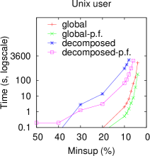
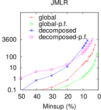
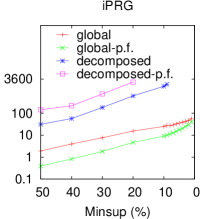
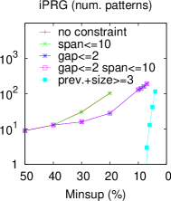
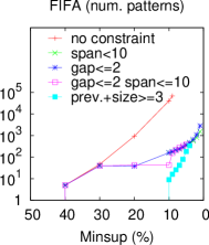
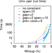
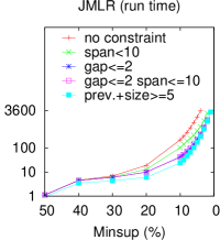
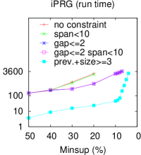
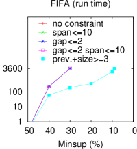
We now evaluate the impact of user constraints on the number of results and on the execution time (Q3). Fig. 4 shows the number of patterns and the execution times for various combinations of constraints. We can see that adding constraints enables users to control the explosion of the number of patterns, and that the execution times decrease accordingly. The constraint propagation allows early pruning of invalid solutions which effectively compensates the computation time of checking the constraints. For example, on the Unix user dataset, it is not feasible to mine for patterns at 5% minimum frequency without constraints, let alone do something with the millions of patterns found. On the other hand, by adding constraints one can look for interesting patterns at low frequency without being overwhelmed by the number of results (see also later).

Figure 4: Number of patterns (top) and execution times (bottom) for the decomposed model with various combinations of constraints.

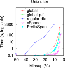
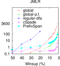
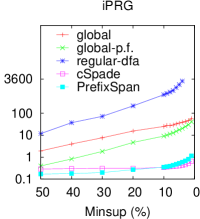
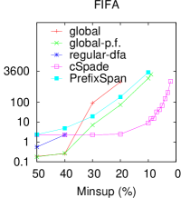
The last experiment compares our models to existing algorithms. Fig. 5 shows the execution times for our global model compared with regular-dfa, PrefixSpan and cSpade (Q4). First, we can observe that regular-dfa is always slowest. On iPRG it performs reasonably well, but the number of transitions in the DFAs does not permit it to perform well on datasets with a large alphabet or large transactions, such as Unix user, JMLR or FIFA. Furthermore, it can not make use of projected frequencies.

global shows similar, but much faster, behaviour than regular-dfa. On datasets with many symbols such as JMLR and FIFA, we can see that not using projected frequency is a serious drawback; indeed, global-p.f. performs much better than global there.

Of the specialised algorithms, cSpade performs better than PrefixSpan; it is the most advanced algorithm and is the fastest in all experiments (not counting the highest frequency thresholds). global-p.f. has taken inspiration from PrefixSpan and we can see that they indeed behave similarly. Although, for the dense iPRG dataset PrefixSpan performs better than global-p.f. and inversely for the large and sparse FIFA dataset. This might be due to implementation choices in the CP solver and PrefixSpan software.

Figure 5: Global model vs. other approaches. Execution times. (Timeout 1 hour.)

Analysis of the pattern quality

Finally, we use our constraint-based framework to perform exploratory analysis of the Unix user datasets. Table 2 shows different settings we tried and patterns we found interesting. Few constraints lead to too many patterns while more constrained settings lead to fewer and more interesting patterns.

setting	# of patterns	interesting pattern	comment
${\bf F_{1}}$	627	-	Too many patterns
${\bf F_{2}}$	512	-	Long sequences of $\mathrm{cd}$ and $\mathrm{ls}$
${\bf F_{3}}$	36	$\mathrm{\langle{\mathrm{{\tt latex,bibtex,latex}}}\rangle}$	User2 is using Latex to write a paper
${\bf D_{1}}$	7	$\mathrm{\langle{\mathrm{{\tt emacs}}}\rangle}$	User2 uses $Emacs$, his/her collaborators use $vi$
${\bf D_{2}}$	9	$\mathrm{\langle{\mathrm{{\tt quota,rm,ls,quota}}}\rangle}$	User is out of disc quota

Table 2: Patterns with various settings (User 2): ${\bf F_{1}}$: $minfreq=5\%$,   ${\bf F_{2}}$: $~{}{\bf F_{1}}\land min\mbox{-}size=3$,   ${\bf F_{3}}$: ${\bf F_{2}}\land max\mbox{-}gap=2\land max\mbox{-}span=5$,   ${\bf D_{1}}$: $minfreq=5\%\land discriminant=8$ (w.r.t. all other users), ${\bf D_{2}}$: $minfreq=0.4\%\land discriminant=8\land member({\mathrm{quota}})$

7 Related work

The idea of mining patterns in sequences dates from earlier work by Agrawal et al. [1] shortly after their well-known work on frequent itemset mining [2]. The problem introduced in [1] consisted of finding frequent sequences of itemsets; that is: sequences of sets included in a database of sequences of sets. Mining sequences of individual symbols was introduced later by [9]; the two problems are closely related and one can adapt one to the other [16]. Sequence mining was driven by the application of market basket analysis for customer data spread over multiple days. Other applications include bio-medical ones where a large number of DNA and protein sequence datasets are available (e.g. [18]), or natural language processing where sentences can be represented as sequences of words (e.g. [15]).

Several specialised algorithm have addressed the problem of constrained sequence mining. The cSpade algorithm [19] for example is an extension of the Spade sequence mining algorithm [20] that supports constraints of type 1, 2 and 3. PrefixSpan [6] mentions regular expression constraints too. The LCMseq algorithm [13] also supports a range of constraints, but does not consider all embeddings during search. Other sequence mining algorithms have often focussed on constraints of type 4, and on closed sequence mining in particular. CloSpan [17] and Bide [16] are both extentions of PrefixSpan to mine closed frequent sequences. We could do the same in our CP approach by adding constraints after each solution found, following [11, 8].

Different flavors of sequence mining have been studied in the context of a generic framework, and constraint programming in particular. They all study constraints of type 1, 2 and 4. In [3] the setting of sequence patterns with explicit wildcards in a single sequence is studied: such a pattern has a linear number of embeddings. As only a single sequence is considered, frequency is defined as the number of embeddings in that sequence, leading to a similar encoding to itemsets. This is extended in [7] to sequences of itemsets (with explicit wildcards over a single sequence). [8] also studies patterns with explicit wildcards, but in a database of sequences. Finally, [10] considers standard sequences in a database, just like this paper; they also support constraints of type 3. The main difference is in the use of a costly encoding of the inclusion relation using non-deterministic automata and the inherent inability to use projected frequency.

8 Conclusion and discussion

We have investigated a generic framework for sequence mining, based on constraint programming. The difficulty, compared to itemsets and sequences with explicit wildcards, is that the number of embeddings can be huge, while knowing that one embedding exists is sufficient.

We proposed two models for the sequence mining problem: one in which the exists-embedding relation is captured in a global constraint. The benefit is that the complexity of dealing with the existential check is hidden in the constraint. The downside is that modifying the inclusion relation requires modifying the global constraint; it is hence not generic towards such constraints. We were able to use the same projected frequency technique as well-studied algorithms such as PrefixSpan [6], by altering the global exists-embedding constraint and using a specialised search strategy. Doing this does amount to implementing specific propagators and search strategies into a CP solver, making the problem formulation not applicable to other solvers out-of-the-box. On the other hand, it allows for significant efficiency gains.

The second model exposes the actual embedding through variables, allowing for more constraints and making it as generic as can be. However, it has extra overhead and requires a custom two-phased search strategy.

Our observations are not just limited to sequence mining. Other pattern mining tasks such as tree or graph mining also have multiple (and many) embeddings, hence they will also face the same issues with a reified exists relation. Whether a general framework exists for all such pattern mining problems is an open question.

Acknowledgments

The authors would like to thank Siegfried Nijssen, Anton Dries and Rémi Coletta for discussions on the topic, and the reviewers for their valuable comments. This work was supported by the European Commission under project FP7-284715 “Inductive Constraint Programming” and a Postdoc grant by the Research Foundation – Flanders.

Appendix

Appendix 0.A Branching with projected frequency

We want to branch only over the symbols that are still frequent in the prefix-projected sequences. Taking the current partially assigned sequence into account, after projecting this prefix away from each transaction, some transactions will be empty and others will have only some subset of its original symbols left.

For each propagator ${\bf C_{i}}\leftrightarrow\exists e~{}\mbox{s.t.}~{}{\bf S}\sqsubseteq_{e}T_{i}$ we maintain the (monotonically decreasing) set of symbols for that transaction in a variable ${\bf X_{i}}$. The propagator in Algorithm 1 needs just a one line addition, that is, after line 12 we add the following:

propagate by removing from ${\bf X_{i}}$ all symbols not in $\langle T_{i}[pos_{e}]..T_{i}[|T_{i}|]\rangle$ except $\epsilon$

which removes all symbols from ${\bf X_{i}}$ that do not appear after the current prefix.

The brancher than first computes the local frequency of each symbol across all ${\bf X_{i}}$, and only branches on the frequent ones. Let $\theta$ be the minimum frequency threshold, then the branching algorithm is the following:

Algorithm 2 local-frequency-brancher$({\bf S},{\bf X})$

1:$pos_{S}\leftarrow$ position of first unassigned variable in ${\bf S}$

2:for $s$ in ${\bf S}[pos_{S}]$ do

3:    $count\leftarrow 0$

4:    for all ${\bf X_{i}}$ do

5:        if $s\in D({\bf X_{i}})$ then $\triangleright$ symbol in domain of ${\bf X_{i}}$

6:           $count\leftarrow count+1$         

7:    end for

8:    if $count>=\theta$ then

9:        add branch-choice ’${\bf S}=s$’     

10:end for

11:branch over all branch-choices (if any)

Appendix 0.B Decomposition with explicit embedding variables, modeling details

The decomposition consists of two constraints: the $position\mbox{-}match$ constraint and the $is\mbox{-}embedding$ constraint.

0.B.0.1 $position\mbox{-}match$ formulation, part 1

The first constraint needed to enforce
$position\mbox{-}match$ is formally defined as follows:

$$\forall i\in 1,\ldots,n,\forall j\in 1,\ldots,|T_{i}|: \quad({\bf S_{j}}=T_{i}[{\bf E_{ij}}])\lor({\bf E_{ij}}=|T_{i}|+1)$$ (14)

Instead of modeling this with a reified element constraint, we can decompose the element constraint over all values in ${\bf E_{ij}}$ except the no-match value $|T_{i}|+1$:

$$\forall i\in 1,\ldots,n,\forall j\in 1,\ldots,|T_{i}|,\forall x\in 1\ldots|T_{i}|:{\bf E_{ij}}=x\rightarrow{\bf S_{j}}=T_{i}[x]$$ (15)

Observe that in the above formulation $T_{i}[x]$ is a constant, so the reified ${\bf S_{j}}=v$ expressions can be shared for all unique values of $v\in\Sigma$.

Furthermore, using half-reified constraints we need only one auxiliary variable for both ${\bf E_{ij}}=x\rightarrow{\bf B}$ and ${\bf B}\rightarrow{\bf S_{j}}=s$, where the latter can be shared for all unique values of $s\in\Sigma$. This leads to $O(n\cdot k\cdot k)$ half-reified constraints of the former type and $O(k\cdot k)$ auxiliary variables and half-reified constraints of the latter type, with $k=max_{i}(|T_{i}|)$.

0.B.0.2 $position\mbox{-}match$ formulation, part 2

The second constraint needed to enforce
$position\mbox{-}match$ is:

$$\forall i\in 1,\ldots,n,\forall j\in 2,\ldots,|T_{i}|: \quad({\bf E_{i(j-1)}}<{\bf E_{ij}})\lor({\bf E_{ij}}=|T_{i}|+1)$$ (16)

Formulating this in CP would not perform any propagation until $|T_{i}|+1$ is removed from the domain of ${\bf E_{ij}}$. However, one can see that the lower-bound on ${\bf E_{i(j-1)}}$, when not equal to $|T_{i}|+1$, can be propagated to the lower-bound of ${\bf E_{ij}}$.

Consider the following example: let $S=[\{B,C,\epsilon\},\{A,B,C,\epsilon\},\{A,B,C,\epsilon\}]$ and $T_{1}=[A,B,C]$ then $k=3$ and $D(E_{1})=\{2,3,4\},D(E_{2})=\{2,3,4\},D(E_{3})=\{2,3,4\}$. However, because $min(D(E_{1}))=2$ we know that $E_{2}\neq 2$ and similar for $E_{3}$. This leads to $E_{3}=\{4\}$, from which the $is\mbox{-}embedding$ propagator can derive that there is no embedding of the pattern in $T_{1}$. This is a quite common situation.

This propagation can be obtained with the following decomposition over all elements of the domain (except $|T_{i}|+1$):

$$\forall i\in 1\ldots n,\forall j\in 1\ldots|T_{i}|-1,\forall x\in 1\ldots|T_{i}|:({\bf E_{ij+1}}=x)\rightarrow({\bf E_{ij}}<x)$$ (17)

However, this would require in the order $O(n\cdot k^{2})$ reified constraints and auxiliary variables.

Instead, we use a simple modification of the binary inequality propagator $X<Y$ that achieves the same required result. This propagator always propagates the lower-bound of $X$ to $Y$, and as soon as $|T_{i}|+1\notin Y$ it propagates like a standard $X<Y$ propagator.

There are $O(n\cdot k)$ such constraints needed and no auxiliary variables.

0.B.0.3 $is\mbox{-}embedding$ formulation

The constraint is the following:

$$\forall i\in 1,\ldots,n:\quad{\bf C_{i}}\leftrightarrow\forall j\in 1,\ldots,|T_{i}|:~{}({\bf S_{j}}\neq\epsilon)\rightarrow({\bf E_{ij}}\neq|T_{i}|+1)$$ (18)

Across all transactions, the reified ${\bf S_{j}}\neq\epsilon$ expressions can be shared. $O(n\cdot k)$ such constraints and auxiliary variables are needed in total. For each transaction, the forall requires $|T_{i}|$ times 2 auxiliary variables, one for reifying ${\bf E_{ij}}\neq|T_{i}|+1$ and one for reifying the implication. This leads to an additional $O(n\cdot k)$ auxiliary variables and constraints, plus $n$ reified conjunction constraints.

Appendix 0.C Sub-search for the existence of a valid ${\bf E_{i}}$

For each transaction $i$ independently, we can search for a valid assignment of the $E_{i}$ variables. As soon as a valid one is found, the sub search can stop and propagate the corresponding assignment to the ${\bf C_{i}}$ and ${\bf E_{i}}$ variables of the master problem.

The following pseudo-code describes how we implemented this scheme as a brancher in a copying solver (implementation for a trailing solver is similar):

Algorithm 3 sub-search-brancher$({\bf C},{\bf E})$

1:substate $\leftarrow$ copy of the current search state

2:for all ${\bf C_{i}}$ do

3:    remove all other branchers (e.g. variable/value orderings)

4:    add to substate the variable/value ordering that tries ${\bf C_{i}}=$true before ${\bf C_{i}}=$false

5:    add to substate as next variable/value ordering to search over all ${\bf E_{ij}}$ variables in lexicographic order, trying their smallest value first

6:    solve substate

7:    if substate has a solution then

8:        save substate’s assignment of ${\bf C_{i}}$ and ${\bf E_{i}}$

9:    else

10:        fail the master problem $\triangleright$ When no valid ${\bf C_{i}}$,${\bf E_{i}}$ can be found     

11:end for

12:merge all saved assignments and have this as the only resulting branch-choice for the master problem

In the above algorithm, for each transaction $i$ we enter the loop and remove all branchers, meaning that there are currently no search choices for the subproblem. We then force the sub-search to only search over ${\bf C_{i}}$ and ${\bf E_{i}}$, such that an assignment for ${\bf C_{i}}=$true is found first, if it exists. By removing all branchers at the start of loop, the next transaction’s sub-search will not reconsider branching choices made in the previous sub-search.

As the master problem should not branch over any of the sub-search choices either, we merge all the assignments found by the sub-searches and present this as the only branch-choice for the master problem.

Using this sub-search-brancher, for each ${T_{i}}$ for which an embedding of ${\bf S}$ in ${T_{i}}$ exists, ${\bf C_{i}}$ will be true. Only if no such embedding exists will ${\bf C_{i}}$ be false. This is the required behaviour for our constraint formulation.

Appendix 0.D Projected frequency for explicit embedding variables

We introduced the following constraint specification:

$$\forall j\in 1\ldots n,x\in\Sigma,\quad{\bf S_{j}}=x\rightarrow|\{i:{\bf C_{i}}\wedge T_{i}[{\bf E_{ij}}]=x\}|\geq\theta$$ (19)

A naive formulation of this expression would require reifying an element constraint ${\bf B}\leftrightarrow T_{i}[{\bf E_{ij}}]=x$. Instead, we will create element constraints $T_{i}[{\bf E_{ij}}]={\bf A_{ij}}$, where ${\bf A_{ij}}$ is an auxiliary integer variable. This leads to the following more efficient reformulation:

$$\forall i\in 1\ldots n,j\in 1\ldots|T_{i}|,\quad T_{i}[{\bf E_{ij}}]={\bf A_{ij}}$$ (20)

$$\forall i\in 1\ldots n,j\in 1\ldots|T_{i}|,x\in\Sigma,\quad {\bf S_{j}}=x\rightarrow|\{i:{\bf C_{i}}\wedge{\bf A_{ij}}=x\}|\geq\theta$$ (21)

References

- [1] Agrawal, R., Srikant, R.: Mining sequential patterns. In: Data Engineering, 1995. Proceedings of the Eleventh International Conference on. pp. 3–14. IEEE (1995)
- [2] Agrawal, R., Srikant, R., et al.: Fast algorithms for mining association rules in large database. In: Proc. 20th Int. Conf. Very Large Data Bases, VLDB. vol. 1215, pp. 487–499 (1994)
- [3] Coquery, E., Jabbour, S., Sais, L., Salhi, Y.: A sat-based approach for discovering frequent, closed and maximal patterns in a sequence. In: European Conference on Artificial Intelligence (ECAI). p. 258–263 (2012)
- [4] Fannes, T., Vandermarliere, E., Schietgat, L., Degroeve, S., Martens, L., Ramon, J.: Predicting tryptic cleavage from proteomics data using decision tree ensembles. Journal of Proteome Research 12(5), 2253–2259 (2013), http://pubs.acs.org/doi/abs/10.1021/pr4001114
- [5] Guns, T., Nijssen, S., De Raedt, L.: Itemset mining: A constraint programming perspective. Artificial Intelligence 175(12-13), 1951–1983 (2011)
- [6] Han, J., Pei, J., Mortazavi-Asl, B., Pinto, H., Chen, Q., Dayal, U., Hsu, M.: Prefixspan: mining sequential patterns efficiently by prefix-projected pattern growth. ICDE’2001, April pp. 215–24 (2001)
- [7] Jabbour, S., Sais, L., Salhi, Y.: Boolean satisfiability for sequence mining. In: 22nd International Conference on Information and Knowledge Management(CIKM’13). pp. 649–658. ACM Press, San Francisco, CA, USA (oct 2013)
- [8] Kemmar, A., Ugarte, W., Loudni, S., Charnois, T., Lebbah, Y., Boizumault, P., Cremilleux, B.: Mining relevant sequence patterns with cp-based framework. In: Tools with Artificial Intelligence (ICTAI), 2013 IEEE 25th International Conference on. IEEE (2014)
- [9] Mannila, H., Toivonen, H., Inkeri Verkamo, A.: Discovery of frequent episodes in event sequences. Data Mining and Knowledge Discovery 1(3), 259–289 (1997)
- [10] Métivier, J.P., Loudni, S., Charnois, T.: A constraint programming approach for mining sequential patterns in a sequence database. In: ECML/PKDD 2013 Workshop on Languages for Data Mining and Machine Learning (2013)
- [11] Negrevergne, B., Dries, A., Guns, T., Nijssen, S.: Dominance programming for itemset mining. In: International Conference on Data Mining (ICDM) (2013)
- [12] Nijssen, S., Guns, T., De Raedt, L.: Correlated itemset mining in ROC space: A constraint programming approach. In: Flach, P., Zaki, M. (eds.) Proceedings of the 15th ACM SIGKDD International Conference on Knowledge Discovery and Data Mining, ACM SIGKDD International Conference on Knowledge Discovery and Data Mining, Paris, France, 28 June - 1 July 2009. pp. 647–656. ACM Press (Jun 2009)
- [13] Ohtani, H., Kida, T., Uno, T., Arimura, H., Arimura, H.: Efficient serial episode mining with minimal occurrences. In: ICUIMC. pp. 457–464 (2009)
- [14] Rojas, W.U., Boizumault, P., Loudni, S., Crémilleux, B., Lepailleur, A.: Mining (soft-) skypatterns using dynamic CSP. In: Integration of AI and OR Techniques in Constraint Programming - 11th International Conference, CPAIOR 2014, Cork, Ireland, May 19-23, 2014. Proceedings. pp. 71–87 (2014)
- [15] Tatti, N., Vreeken, J.: The long and the short of it: summarising event sequences with serial episodes. In: KDD. pp. 462–470 (2012)
- [16] Wang, J., Han, J.: Bide: Efficient mining of frequent closed sequences. In: Data Engineering, 2004. Proceedings. 20th International Conference on. pp. 79–90. IEEE (2004)
- [17] Yan, X., Han, J., Afshar, R.: Clospan: Mining closed sequential patterns in large datasets. In: Proceedings of SIAM International Conference on Data Mining. pp. 166–177 (2003)
- [18] Ye, K., Kosters, W.A., IJzerman, A.P.: An efficient, versatile and scalable pattern growth approach to mine frequent patterns in unaligned protein sequences. Bioinformatics 23(6), 687–693 (2007)
- [19] Zaki, M.J.: Sequence mining in categorical domains: incorporating constraints. In: Proceedings of the ninth international conference on Information and knowledge management. pp. 422–429. ACM (2000)
- [20] Zaki, M.J.: Spade: An efficient algorithm for mining frequent sequences. Machine Learning 42(1), 31–60 (2001)