Spectral unmixing of Multispectral Lidar signals
Abstract
In this paper, we present a Bayesian approach for spectral unmixing of multispectral Lidar (MSL) data associated with surface reflection from targeted surfaces composed of several known materials. The problem addressed is the estimation of the positions and area distribution of each material. In the Bayesian framework, appropriate prior distributions are assigned to the unknown model parameters and a Markov chain Monte Carlo method is used to sample the resulting posterior distribution. The performance of the proposed algorithm is evaluated using synthetic MSL signals, for which single and multi-layered models are derived. To evaluate the expected estimation performance associated with MSL signal analysis, a Cramer-Rao lower bound associated with model considered is also derived, and compared with the experimental data. Both the theoretical lower bound and the experimental analysis will be of primary assistance in future instrument design.
Index Terms:
Remote sensing, Multispectral Lidar, Spectral unmixing, Estimation performance, Bayesian estimation, Markov Chain Monte Carlo.I Introduction
Laser altimetry (or Lidar) is an acknowledged tool for extracting spatial structures from three-dimensional (3D) scenes, including forest canopies [Mallet2009, Leeuwen2010]. Using time-of-flight to create a distance profile, signal analysis can recover tree and canopy heights, leaf area indices (LAIs) and ground slope by analyzing the reflected photons from a target. Conversely, passive multispectral (MSI) (dozen of wavelengths) and hyperspectral images (HSI) (hundreds of wavelengths) are widely used to extract spectral information about the scene which, for forest monitoring, can also provide useful parameters about the canopy composition and health (tree species, leaf chlorophyll content, water content, stress, among others) [Lemaire2008, Hernandez2011]. The most natural evolution to extract spatial and spectral information from sensed scenes is to couple Lidar data and multi/hyperspectral images [Dalponte2008, Buckley2013]. Although the fusion of Lidar data and HSIs can improve scene characterization, there are problems of data synchronization in space (alignment, resolution) and time (dynamic scene, change of observation conditions, etc). For these reasons, multispectral Lidar (MSL) has recently received attention from the remote sensing community for its ability to extract both structural and spectral information from 3D scenes [Wallace2012, Hakala2012].
The key advantage of MSL is the ability to provide information on the vertical distribution of spectra, used to infer physiological processes directly linked to actual carbon sequestration as well as carbon stocks [Wallace2014]. For example, a key capability is to directly measure and classify ground-based shrub infestation, which is difficult with conventional HSI as the lower spectral response is obscured by the ’first’ signals returned from the top of the canopy. Preliminary trials with existing commercial LiDAR systems with three operational wavelengths have already taken place [Fleming2015], but as we shall demonstrate here, such systems cannot yet provide all the necessary spectral and structural discrimination to directly measure these processes.
Another motivation for MSL is that HSI, even when fully synchronised, can only integrate the spectral response along the path of each optical ray, not measure the spectral response as a function of distance, e.g. depth into a forest canopy. Multiple scattering effects cannot be neglected in some scenes with relief or containing multi-layered objects (such as trees), which complicates surface detection and quantification. Most existing spectral unmixing (SU) techniques rely on a linear mixture assumption [Craig1994, Heinz2001, Eches2010a, Miao2007a, Yang2011] to identify the components (so-called endmembers) of an image and their proportions (abundances). However, it has been shown that the classical linear mixing model (LMM) can be inaccurate when multiple scattering effects occur [Keshava2002, Bioucas2012]. Although polynomial models [Altmann2012a, Altmann2014a] (including bilinear models[Somers2009, Nascimento2009, Fan2009, Halimi2010]) can be adapted for “long range” multiple scattering (in contrast to intimate mixtures models [Hapke1981]), motivating the additional parameter constraints and designing accurate nonlinear unmixing methods are still challenging problems [Dobigeon2014]. Since MSL data present an additional dimension when compared to HSIs, we can expect a reduction of the SU problem complexity and thus an improvement in the target characterization performance.
In [Hernandez2007], the authors proposed a Bayesian algorithm to estimate the positions and amplitudes in Lidar signals associated with a multi-layer target. This method has been extended in [Ramirez2012, Wallace2014] to MSL by first estimating the positions of the peaks (i.e., the layers), which were assumed to be the same in all spectral bands, then estimating the amplitudes of the peaks for each wavelength, and finally relating the estimated amplitude peaks to areas associated with each material that make up the target based on a linear mixing model. The method has been applied to real MSL signals (four wavelengths) to analyze a conifer structure and has been shown to aid the recovery of bark and needle areas of the tree assuming it is modeled as a set of irregularly spaced layers.
In this paper, we propose to investigate a SU problem applied to single- and multi-layered targets to estimate the positions and proportions of each (known) material. This problem extends the supervised SU problem of HSIs by also estimating the target position. Estimating the spectral variation of material signatures (unsupervised SU problem) is also of interest. For example, the estimation of physiological content, such as Chlorophyll concentration, in forest canopies is of key concern, and this results in variable spectra for leaves and needles. Extracting these spectra from MSL signals is a more challenging problem (probably more difficult than in HSIs due to the statistical properties of the noise and observation model) which is out of scope of this paper, but will require particular attention in future work.
In contrast with the classical additive Gaussian noise assumption used for HSIs, a Poisson noise model is more appropriate for MSL signals. Indeed, Lidar and thus MSL systems usually record, for each pixel/region of the scene, a histogram of time delays between emitted laser pulses and the detected photon arrivals. Within each histogram bin, the number of detected photons follows a discrete distribution which can be approximated by a Poisson distribution due to the particle nature of light. Using a Bayesian approach, appropriate prior distributions are chosen for the unknown parameters of the model considered here, i.e., the material areas, the surface positions and the background parameters. The joint posterior distribution of these parameters is then derived. Since the classical Bayesian estimators cannot be easily computed from this joint posterior (mainly due to the model complexity), a Markov chain Monte Carlo (MCMC) method is used to generate samples according to the posterior of interest.
More precisely, following the principles of the Gibbs sampler, samples are generated according to the conditional distributions of the posterior. Due to the possibly high correlations between the material proportions/areas, we propose to use a Hamiltonian Monte Carlo (HMC) [Duane1987] method to sample according to some of the conditional distributions. HMCs are powerful simulation strategies based on Hamiltonian dynamics which can improve the convergence and mixing properties of classical MCMC methods (such as the Gibbs sampler and the Metropolis-Hastings algorithm) [Brooks2011, Robert2004]. These methods have received growing interest in many applications, especially when the number of parameters to be estimated is large [Neal1996, schmidt09funcfact]. Classical HMC can only be used for unconstrained variables. However, new HMC methods have been recently proposed to handle constrained variables [Brooks2011, Chap. 5], [Hartmann2005, Brubaker2012] which allow HMCs to sample according to the posterior of the Bayesian model proposed for SU. Finally, as in any MCMC method, the generated samples are used to compute minimum mean square error (MMSE) estimators as well as measures of uncertainties such as confidence intervals.
Predicting the parameter estimation performance is of prime interest for designing an estimation procedure but also assists with the instrument design. Indeed, since MSL is a recent modality, it is important to identify the key parameters that have an influence on the material estimation performance (such as the necessary signal to background levels, the number of bands to be considered and the associated wavelengths). To guide future instrument design, we consider a Cramer-Rao lower bound (CRLB) associated with the observation model and show that it can be used to approximate the estimation errors of the proposed Bayesian algorithm.
The remainder of the paper is organized as follows. Section II introduces the observation model associated with MSL returns for a single-layered object to be analyzed. Section III presents the hierarchical Bayesian model associated with the proposed model and its posterior distribution. The hybrid MCMC method used to sample from the posterior of interest is detailed in Section IV. Section V investigates the expected SU performance using Cramer-Rao lower bounds. Experimental results are shown and discussed in Section VI. Conclusions are reported in Section LABEL:sec:conclusion.
II Problem formulation
This section introduces the observation statistical model associated with MSL returns for a single-layered object which will be used in Sections III and IV to solve the SU problem of MSL data. Precisely, we consider a set of observed Lidar waveforms where is the number of temporal (corresponding to range) bins. To be precise, is the photon count within the th bin of the th spectral band considered. Let be the position of a complex object surface or surfaces at a given range from the sensor, composed of materials whose spectral signatures (observed at wavelengths) are denoted as . According to [Hernandez2007], each photon count is assumed to be drawn from the following Poisson distribution
| (1) |
where is the photon impulse response whose shape can differ between wavelength channels, denotes the area of the th material composing the object (relative to a reference area) and is a background and dark photon level, which is constant in all bins at a given wavelength. Without loss of generality the photon impulse responses are assumed to be the same and modeled by the following piece-wise exponential
| (6) |
where is a positive hyperparameter vector. In this study, we assume that the shape parameters of the model (which is appropriate for our own lidar sensors) are fixed and known from the instrumental response. As seen later in Fig. 3 the shape is slightly asymmetrical when compared to the more common Gaussian model [Wagner2006] which is used for higher power, longer pulse duration lidar systems. The consideration of a piece-wise exponential approximation is motivated by the actual shape of our instrumental impulse response but it is worth mentioning that any positive analytical approximation, even different approximations for the different wavelengths, could be used instead without modifying the proposed Bayesian estimation procedure. The consideration of a single impulse response model is done only for ease of reading. While a Gaussian approximation can lead to a slight bias in depth estimation, we shall use a Gaussian approximation in Section V to compute the Cramer-Rao bounds since the Gaussian approximation is twice differentiable (in contrast to the piece-wise exponential approximation), which simplifies the derivation of the bounds.
Due to physical considerations, the relative areas are assumed to satisfy the following positivity constraints
| (7) |
Similarly, the average background level in each channel satisfies . Spectral unmixing of the MSL data consists of estimating the position (i.e., ) of the target, the area of each component of the target, as well as the background levels from the observed data in . The next section studies a Bayesian model to estimate the unknown parameters in (1) while ensuring the positivity constraints mentioned above.
III Bayesian model
The unknown parameter vector associated with (1) contains the relative areas , the position of the target and background levels (satisfying positivity constraints). This section summarizes the likelihood and the parameter priors associated with these parameters.
III-A Likelihood
Assuming that the detected photon counts/noise realizations, conditioned on their mean in all bins and for all wavelengths, are independent, Eq. (1) leads to
| (8) |
where , and denotes the th row of .
III-B Prior for the target position
Since we don’t have prior information about the position of the target, the following uniform distribution
| (9) |
is assigned to . Note that the position is a real variable that is not restricted to the integer values in .
III-C Prior for the relative areas
To reflect the lack of prior knowledge about the areas, the following truncated Gaussian prior
| (10) |
is assigned to each area , where denotes the Gaussian distribution restricted to , which hidden mean and variance and , respectively. The hyperparameter is shared by all the parameters and is arbitrarily fixed to a large value to ensure a weakly informative prior. Assuming prior independence for the unknown areas yields
| (11) |
where means ”proportional to” and is the indicator function defined on .
III-D Prior for the background level
Similarly, assigning a truncated Gaussian prior to each background level and assuming prior independence between these parameters leads to
| (12) |
where the hyperparameter is shared by all the parameters and is arbitrarily fixed to a large value to ensure a weakly informative prior.
In this paper, we assume that prior knowledge about the relative areas and background levels is limited. We use weakly informative Gaussian priors restricted to the positive orthant to reflect this lack of knowledge and reduce the estimation bias while ensuring the positivity constraints are satisfied. However any proper weakly informative prior distributions could have been used, leading to similar estimation results. Similarly, if useful information about the unknown parameters is available, more informative (possibly physics-based) priors can be used instead of (9) and (11) (target position and composition) and (12) (background levels).
III-E Joint posterior distribution
The resulting directed acyclic graph (DAG) associated with the proposed Bayesian model is depicted in Fig. 1. The joint posterior distribution of the unknown parameter vector can be computed using
| (13) |
where has been defined in (8) and .
Unfortunately, it is difficult to obtain closed form expressions for standard Bayesian estimators associated with (13). In this paper, we propose to use efficient Markov Chain Monte Carlo (MCMC) methods to generate samples asymptotically distributed according to (13), employing a Gibbs sampler. The principle of the Gibbs sampler is to sample according to the conditional distributions of the posterior of interest [Robert2004, Chap. 10]. Due to the high correlation between the elements of (which will be discussed later in the paper), we use an Hamiltonian Monte Carlo (HMC) method which improves the mixing properties of the sampling procedure (compared to a classical Metropolis-within-Gibbs sampler using Gaussian random walks). This method is detailed in the next section.
IV Bayesian inference using a Constrained Hamiltonian Monte Carlo method
In this Section, we develop an HMC-within Gibbs sampler to generate samples according to (13) and estimate the unknown parameters involved in (1) in order to solve the SU problem of MSL data for a single-layered object. The proposed sampler consists of three steps to update sequentially and and is summarised in Algo. IV-C.
IV-A Sampling the areas
The full conditional distribution of is given by
| (14) |
and is not a standard distribution which is easy to sample. Consequently, it is the norm to use an accept/reject procedure to update . A classical and simple approach would use a multivariate Gaussian random walk. However, in practice the elements of can be highly correlated, especially when the materials present similar spectral signatures (which will be the case for vegetation targets). Consequently, a Hamiltonian Monte Carlo method [Brooks2011, Chap. 5] is preferred to improve the mixing properties of the sampler. The principle of HMCs is to introduce auxiliary, or momentum, variables, and perform a Metropolis-Hastings move in a higher dimensional parameter space. The proposal distribution is then built to take into account the shape of the target distribution (14). Due to the area constraints (7), a constrained HMC must be used. In this paper, we used a constrained HMC (CHMC) scheme similar to that described in [Altmann2014a] and thus consider the following potential energy function
| (15) |
to simulate Hamiltonian dynamics and compute the appropriate acceptance ratio (see [Altmann2014a, Brooks2011] for technical details). This choice of potential energy function ensures that where is a positive constant. Note that the proposed CHMC step can be applied for any differentiable relative area prior. Metropolis-Hastings or more complex HMC moves should be used instead when considering non-differentiable priors instead of (11).
IV-B Sampling the target position
It can be shown from (13) that
| (16) |
is not a standard distribution and an accept/reject procedure must be used to update the target position . We use a Gaussian random walk to update this parameter. More precisely, a doubly truncated Gaussian proposal is considered to ensure each candidate belongs to the admissible set and the variance of the proposal is adjusted during the burn-in period of the sampler to obtain an acceptance rate close to , as recommended in [Robertmcmc, p. 8].
IV-C Sampling the background levels
Sampling from (18) is again not straightforward and Gaussian random walks are used to update the background levels, similar to the position . However the background levels are a posteriori independent and can be updated in parallel. Similar to the target position update, the variances of the parallel Gaussian random walk procedures are set during the burn-in period of the sampler to obtain an acceptance rate close to .
Algorithm 1
Gibbs Sampling Algorithm (single layer)
-
•
Set
After generating samples using the procedures detailed above and removing iterations associated with the burn-in period of the sampler ( has been set from preliminary runs), the MMSE estimator of the unknown parameters can be approximated by computing the empirical averages of the remaining samples. The minimal length of the burn-in period can be determined using several convergence diagnostics [Robertmcmc] but the number of initial samples to be discarded generally varies between data sets and can be thus difficult to adjust in advance without overestimating it. In previous work on parallel acceleration of RJMCMC algorithms we have investigated the application of such diagnostics to our monochromatic LiDAR signals [Ye2013], but as absolute speed of processing is not a major concern here, the length of the burn-in period is assessed visually from the preliminary runs and fixed to ensure that the sampler has converged. The total number of iterations has then been set to obtain accurate approximations (computed over samples in Section VI) of the MMSE estimators.
V Predicting unmixing performance
This section studies a Cramer-Rao lower bound associated with the observation model (1) which can be used to assess the performance of methods that aim to solve the SU problem of MSL data considered in this paper as well as to assist with the future instrument design. Precisely, Section V-A recalls the definition of the CRLB for the problem of interest and Section V-B discusses the impact of several key parameters on the expected parameter estimation performance of SU methods.
V-A Cramer-Rao lower bound
Prediction of the unmixing performance is necessary to assist in the design of a lidar system for a specific application, identifying those parameters that have the most significant impact. In deriving a CRLB, we propose firstly to relax the impulse response model in (6) by considering the following Gaussian approximation
| (19) |
This simplifies the CRLB derivation and does not significantly bias the prediction as the piece-wise exponential impulse response can be accurately approximated by a Gaussian function. The CRLB associated with any unbiased estimator of the parameter vector involved in the mixing model (1) (having replaced by ) and constructed from is given by
| (20) |
where is the Fisher information matrix whose elements are111The Fisher information matrix is derived in the Appendix
The th diagonal element of the CRLB matrix in (20) provides a lower bound for the variance of , given that is an unbiased estimator of . Of course, the Bayesian estimation procedure proposed in Sections III and IV does not provide a strictly unbiased estimator of and a Bayesian CRLB should have been considered instead of (20). However, due to the weakly informative priors chosen in Section III, when the actual vector is far enough from the boundaries of the admissible set (defined by the positivity constraints), the bias of the proposed estimation procedure can be neglected and the resulting estimator achieves the CRLB (as will be shown in Section VI). Moreover, the CRLB in (20) can also provide information about the estimation performance of a potential optimization method that could be proposed to estimate based on maximum likelihood estimation (MLE).
V-B Performance analysis
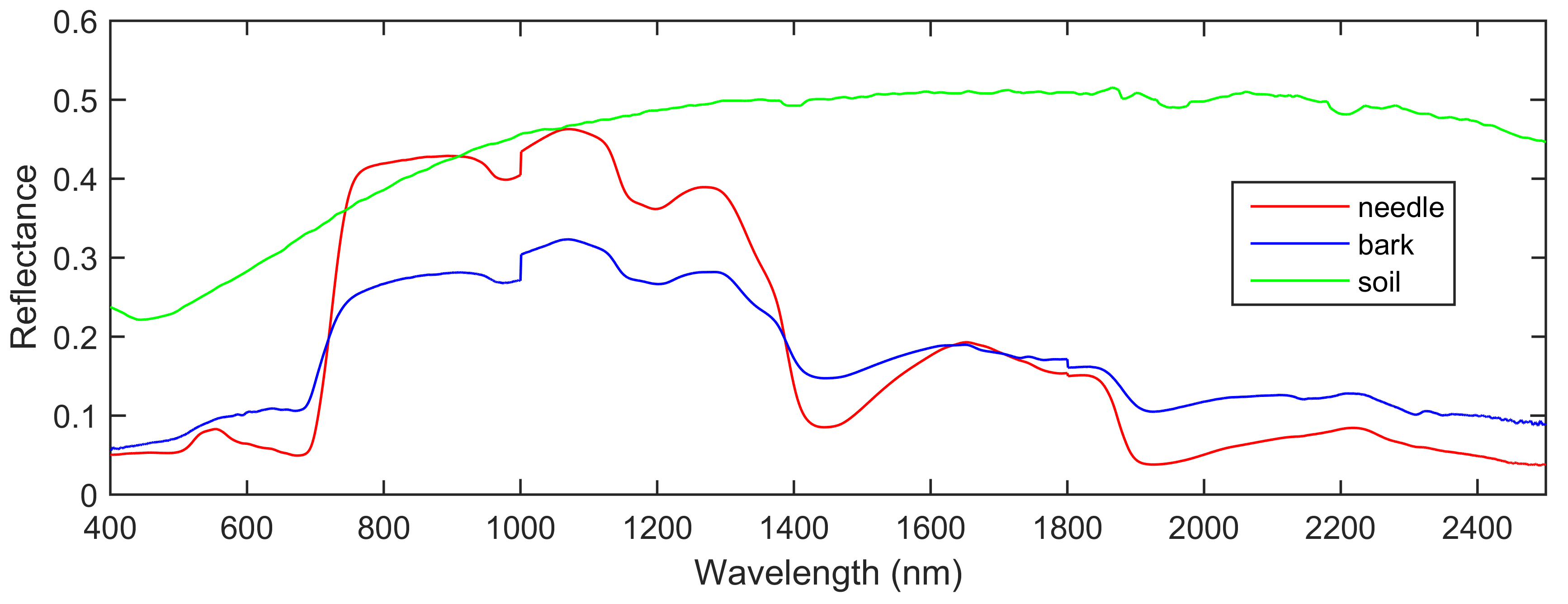
We first investigate the performance of spectral unmixing of MSL signals for a single layered, artificial target composed of materials, specifically needles, bark and soil. These materials have been chosen because of our interests in forest canopy monitoring using MSL signals [Wallace2014]. The reflectance spectra of these materials, observed at equally spaced spectral bands ranging from nm to nm are depicted in Fig. 2. It is interesting to note the strong similarity between the bark and needles spectral signatures, which can make their discrimination difficult and highlights the need of multiple wavelengths to quantify these materials. The maximum number of spectral bands considered in this paper has been set to , which is a realistic value for a short-term real measurement campaign (the current instrument uses only wavelengths). The relative area of needles (resp. bark and soil) has been arbitrarily set to (resp. and ). These relative areas do not necessarily sum to one as we consider that part of the laser light can penetrate through the target (semi-transparent target or a significant gap fraction) and may not be further reflected (single hit assumption). The fixed model parameters have been fixed from experiments to
| (25) |
These parameters will be fixed in the remainder of the paper unless otherwise specified. The impulse response parameters have been set to and for the piece-wise exponential approximation in (6) and for the Gaussian approximation in (19). These parameters have been obtained by fitting the experimental impulse response measured in [Hernandez2007]. Fig. 3 shows that the Gaussian approximation provides a good estimate of the experimental impulse response, although the piece-wise exponential better fits the experimental curve.
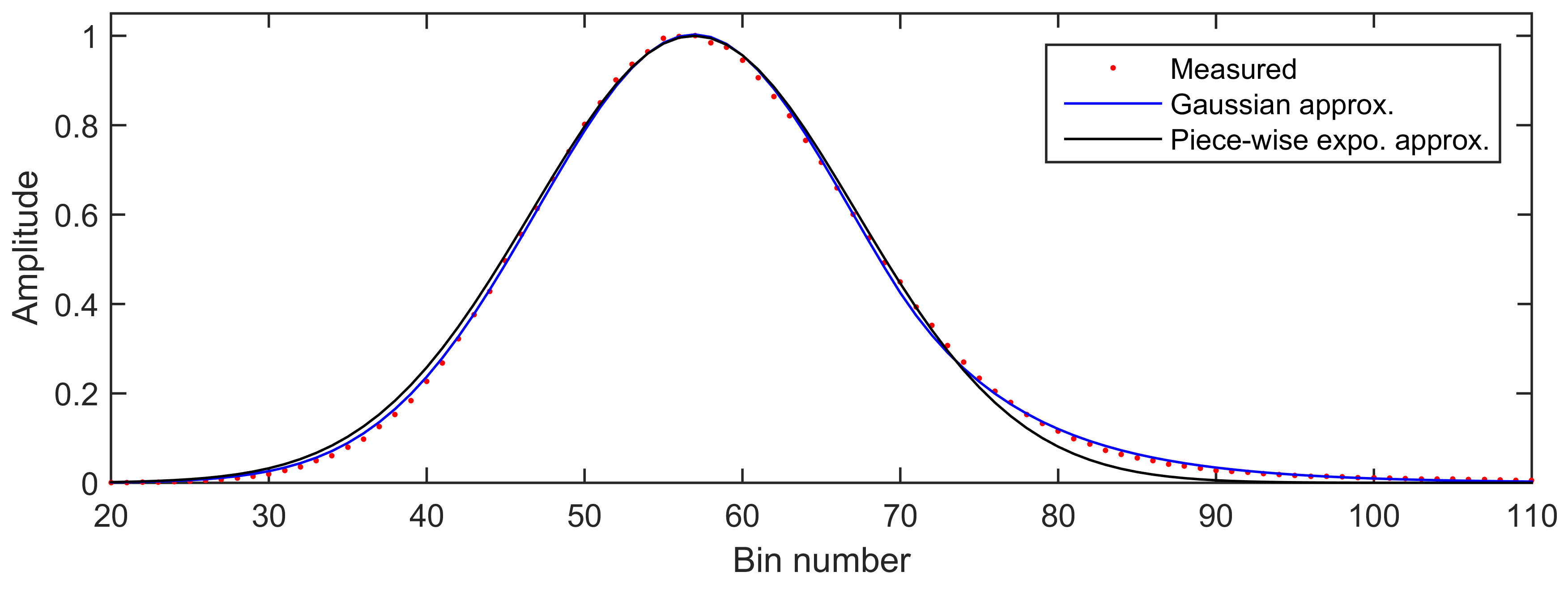
Fig. 4 shows an example of MSL data generated using the parameters in (25) and the impulse response approximation in (6).
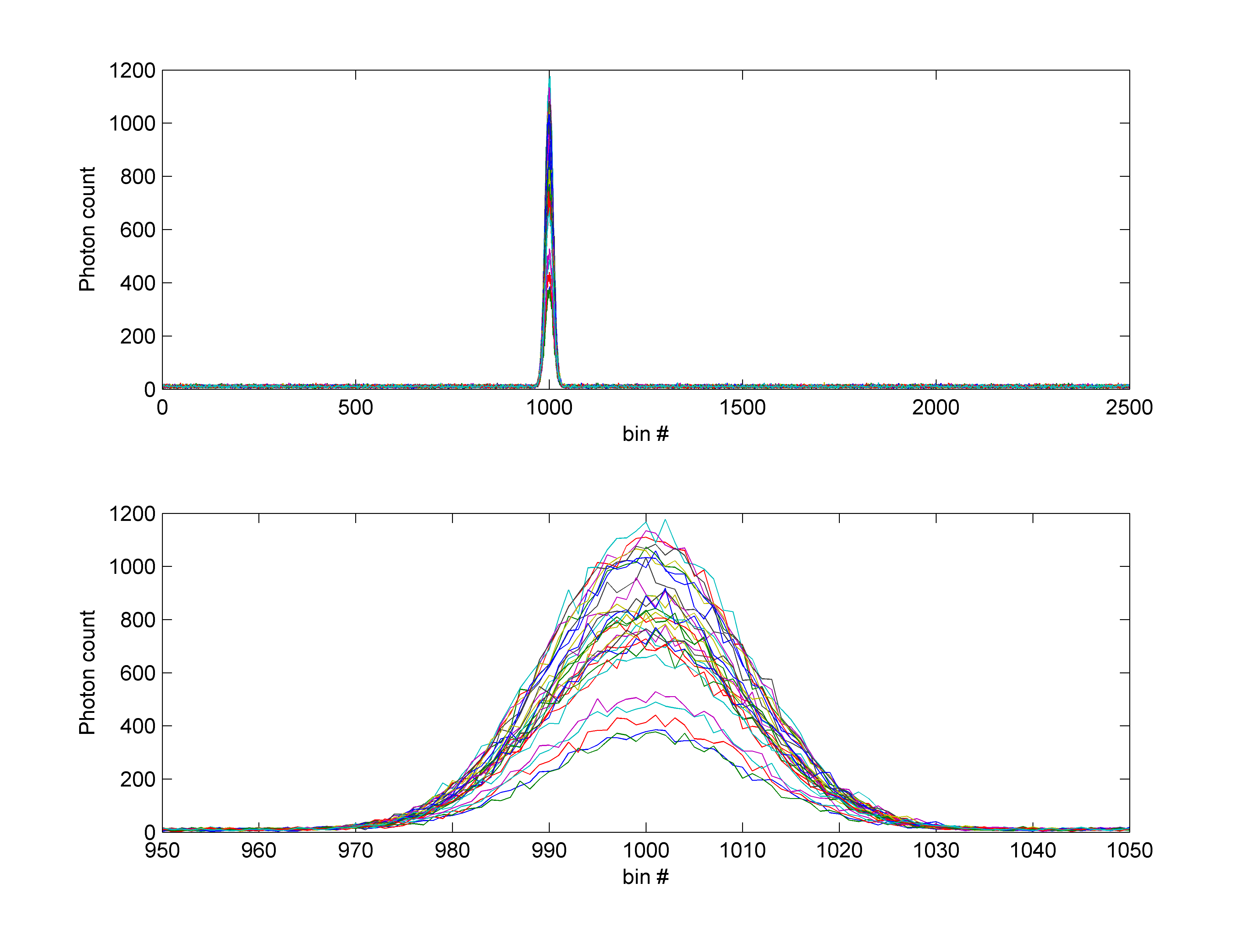
Table I shows the predicted estimation performance for the unknown parameters of interest (i.e., and ) assuming the Gaussian approximation of the photon impulse response (19). The relative errors provided in the bottom row of Table I are computed by dividing the square root of the CRLBs by the actual values of the parameters. The relative estimation errors of the background levels (not presented here) are lower than .
| Actual value | ||||
| CRLB | ||||
| Rel. err. (%) | 8.0 | 10.7 | 1.5 |
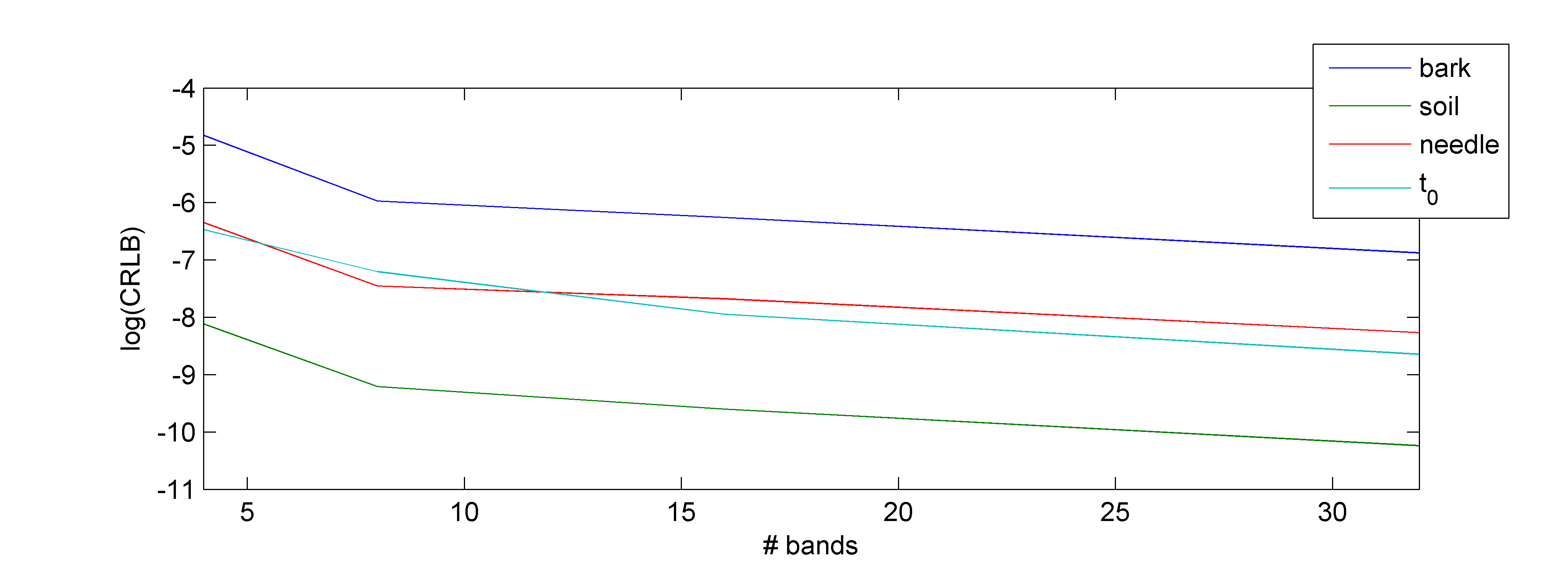
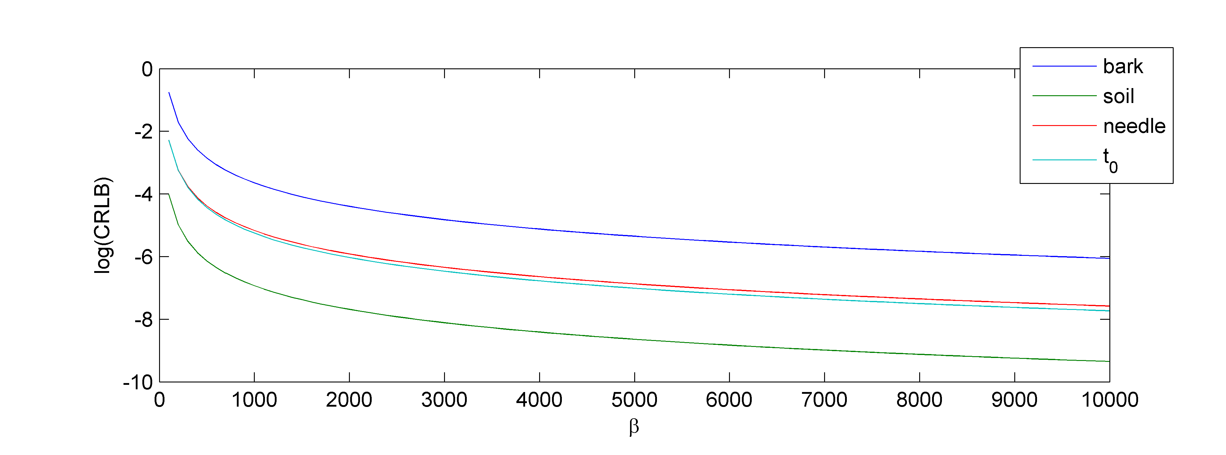
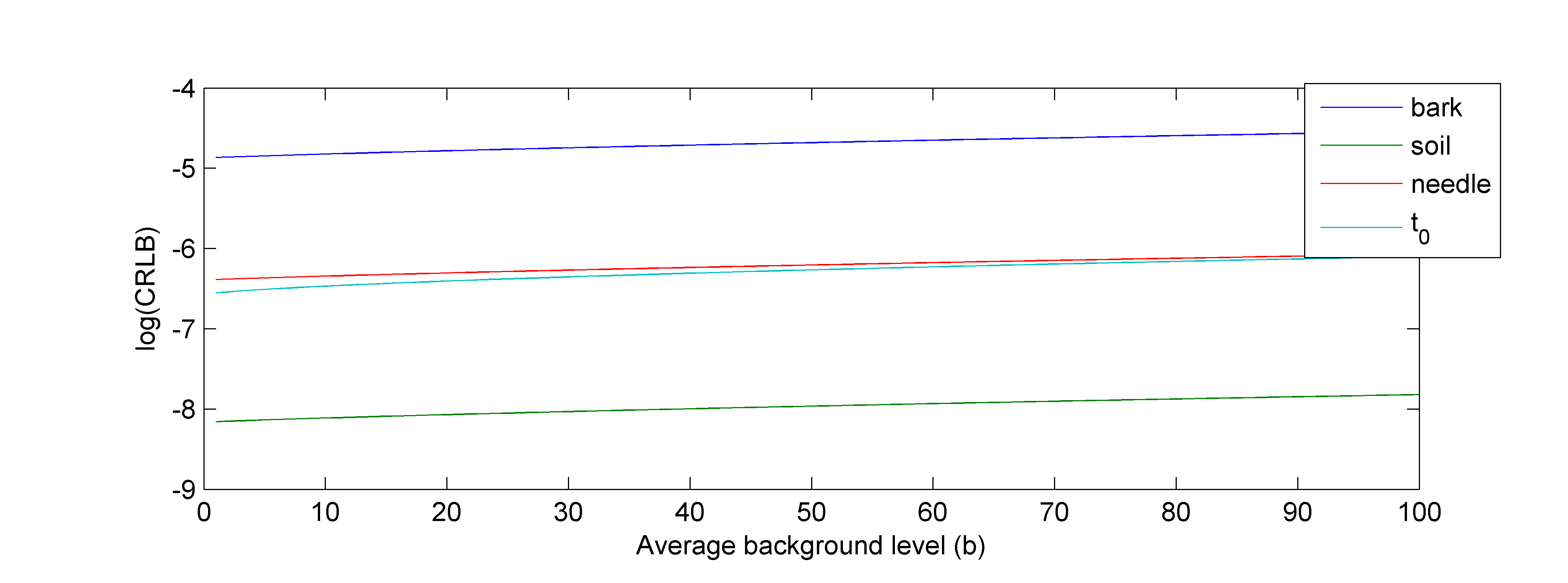
These results show that the estimation errors associated with the target position are usually much lower than those associated with the material areas. Moreover, although the amplitude of the peak for each wavelength is much larger than the background level (see Fig. 4), the CRLB predicts possibly large estimation errors, especially for the needle and bark areas. This can be partially explained by the fact that the soil reflectance spectrum presents an average energy which is higher than those of needles and bark (and thus ) but also and mainly because of the high correlation between the bark and needle spectra, which complicates their quantification. Figs. 5 to 7 show the predicted estimation errors for different values of the key parameters (which is related to the number of photons emitted by the laser sources), the number of spectral bands (equally spaced between nm and nm) and the average background level (assumed to be the same in all spectral bands and bins). Fig. 5 shows that the estimation performance generally increases with the number of spectral bands. This result is well known for SU of multispectral and hyperspectral images and is here demonstrated for MSL signals. However, the performance improvement can vary, depending on the additional spectral bands considered. For instance, additional bands containing similar spectral information may not significantly improve the unmixing results (e.g., several wavelengths between nm and nm for the three materials in Fig. 2). Fig. 6 shows that the parameter has a significant impact on the SU performance. This parameter increases with the amplitude and the number of laser source pulses used to acquire the data and decreases with the average distance between the source and the target (as the probability of recording a reflected photon decreases). Increasing leads to better area estimation but can require a longer target exposure (which can be problematic for airborne sensors for instance). Finally, Fig. 7 shows that for relatively small values of background levels (compared to ), the SU performance is not significantly degraded when the background increases. This background level (which depends primarily on the background (e.g. solar) radiation as well as the instrument design) is expected to be quite small in practice.
VI Experiments
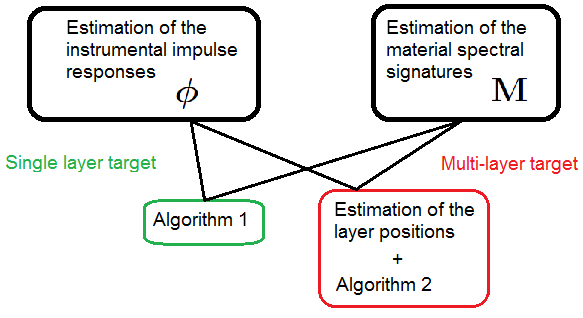
In this section, we first apply (Section VI-A) the proposed SU method to synthetic MSL data associated with a single-layered target and compare its estimation performance to that predicted by the CLRB presented in Section V and to that of a state-of-the art method [Wallace2014]. In Section VI-B, we investigate the case of a multi-layered target whose layer positions are assumed to be known. Although the current algorithm does not estimate the positions of multiple surfaces, Section VI-B aims to illustrate how the proposed method can be extended to analyze more complex objects. The main steps of the methodology (proposed to analyze single and multi-layer target) are summarised in Fig. 8.
VI-A Single layer target
In this section, we evaluate the performance of the proposed spectral unmixing algorithm on synthetic MSL signals generated using the parameters used in Section V-B (Eq. (25)) and impulse response approximation (6).
The number of spectral bands has been chosen as , equally spaced between nm and nm. For each scenario, the number of iterations has been set to (including burn-in samples). The hyperparameters have been fixed to . The estimation performance of the proposed algorithm is evaluated by comparing the CRLB defined in Section V to the mean square error (MSE) defined as
| (26) |
where and are the actual and estimated th element of the unknown parameter vector and the expectation is approximated using Monte Carlo runs. The performance of the proposed algorithm is compared to the CRLB (including the Gaussian approximation (19)) and to the performance of the algorithm developed in [Wallace2014], denoted as “State-of-the-art” and which consists of estimating sequentially the position, amplitudes of the peaks for each wavelength and finally the relative areas.
Table II shows that the MSEs obtained for by the two algorithms are close to the CLRBs, although the proposed algorithm generally outperforms the method proposed in [Wallace2014] due to the joint estimation of the target position and the material areas. Note that for , the variance of the proposed estimator is slightly lower than the CRLB. This can be mainly explained by the fact that the estimator is no longer unbiased in that case. Table III compares the average relative estimation errors obtained by the two algorithms and computed by dividing the square root of the MSEs by the actual values of the parameters. These results show that increasing the number of spectral bands from to almost divides the area estimation errors by three (e.g., from to for the bark area), which highlights the benefits of increasing the number of wavelengths.
| Actual parameter value | ||||
| CRLB | ||||
| Proposed Algo. | ||||
| State-of-the-art | ||||
| CRLB | ||||
| Proposed Algo. | ||||
| State-of-the-art | ||||
| CRLB | ||||
| Proposed Algo. | ||||
| State-of-the-art | ||||
| CRLB | ||||
| Proposed Algo. | ||||
| State-of-the-art | ||||
| Actual parameter value | ||||
| Theo. (%) | 8.0 | 10.7 | 1.5 | |
| Proposed Algo. | 8.2 | 11.0 | 1.5 | |
| State-of-the-art | 8.6 | 11.5 | 1.6 | |
| Theo. (%) | 10.8 | 14.6 | 2.0 | |
| Proposed Algo. | 11.0 | 14.8 | 2.1 | |
| State-of-the-art | 11.6 | 15.7 | 2.2 | |
| Theo. (%) | 12.1 | 16.8 | 2.5 | |
| Proposed Algo. | 12.0 | 16.8 | 2.5 | |
| State-of-the-art | 12.4 | 17.4 | 2.6 | |
| Theo. (%) | 21.0 | 29.9 | 4.3 | |
| Proposed Algo. | 20.0 | 28.8 | 4.2 | |
| State-of-the-art | 21.4 | 30.8 | 4.5 | |
VI-B Extension to a multi-layer target
Algorithm 2
Gibbs Sampling Algorithm (multi-layer)