Thermodynamics of two-dimensional spin models with bimodal random-bond disorder
Abstract
We use numerical linked cluster expansions to study thermodynamic properties of the two-dimensional classical Ising, quantum XY, and quantum Heisenberg models with bimodal random-bond disorder on the square and honeycomb lattices. In all cases, the nearest-neighbor coupling between the spins takes values with equal probability. We obtain the disorder averaged (over all disorder configurations) energy, entropy, specific heat, and uniform magnetic susceptibility in each case. These results are compared with the corresponding ones in the clean models. Analytic expressions are obtained for low orders in the expansion of these thermodynamic quantities in inverse temperature.
pacs:
61.43.-j,05.50.+q,75.10.Jm,05.10.-aI Introduction
Solid-state materials deviate in various ways from the periodic idealizations sometimes used to describe them theoretically. In crystals, for example, such deviations can occur due to the presence of lattice distortions, impurity atoms (that may or may not be magnetic), and vacancies in the lattice, collectively termed as disorder. Disorder can significantly influence material properties. A dramatic example for noninteracting electrons is Anderson localization.Anderson (1958) In spin systems, the focus of this work, quenched disorder in the spin interactions leads to frustration and can generate spin glasses.Binder and Young (1986) A spin glass is a remarkable state of matter where, loosely speaking, spins are “frozen” in an irregular pattern, i.e., they display a very slow dynamics under external driving. Although this phase does not exhibit spin order in a traditional sense (e.g., as a ferromagnet), it is still distinctly different from a paramagnet. Experimentally, spin glasses are generally associated with a cusp in the ac susceptibility at a certain temperature above which the system behaves like a paramagnet.Weissman (1993) Whereas no standard order parameter captures a glassy transition, glass order parameters exist that do so (see, e.g., Refs. Binder and Young, 1986; Katzgraber et al., 2007).
In two-dimensional (2D) lattices (the focus of this work), the effects of quenched disorder on classical spins have been extensively studied over the years.Binder and Young (1986) However, the calculation of thermodynamic properties and correlation functions continues to be a computational challenge.Parisen Toldin et al. (2011); Thomas and Middleton (2013) While it is generally believed that no spin-glass phase exists for nonzero temperatures,Binder and Young (1986) zero-temperature phases continue to be debated for various models of interest (see, e.g., Refs. Thomas et al., 2011; Parisen Toldin et al., 2011). For quantum spin models, the sign problemHenelius and Sandvik (2000); Troyer and Wiese (2005) in quantum Monte Carlo simulations and the exponential growth of the Hilbert space, relevant to full exact diagonalization calculations, represent an even greater challenge. Because of this, the properties of disordered quantum spin systems, and of quantum spin glasses in particular, have remained essentially unexplored. The existing literature in the subject has almost exclusively dealt with classical models.
Our goal in this work is to use a recently introduced numerical linked cluster expansion (NLCE) for disordered systemsTang et al. to study the thermodynamic properties of the classical Ising (with ), and quantum (spin-1/2) XY and Heisenberg models with bimodal random-bond disorder on the square and honeycomb lattices. NLCEs allow us to obtain finite temperature properties of those models in the thermodynamic limit through the exact diagonalization of finite-size clusters. We specifically study the energy, entropy, specific heat, and uniform magnetic susceptibility (for the magnetization in the -direction) as a function of temperature. Since any glassy phase is only expected to emerge at zero temperature in these models, if at all, we do not study the spin-glass order parameter. In future work, we will study quantum quenchesTang et al. ; Rigol (2014a); Wouters et al. (2014); Rigol (2014b) to examine the possibility of disorder driven localization in 2D.
Our results are briefly as follows: For clean systems, they match well with known results for the square lattice, while we report additional results for the honeycomb lattice. For the disordered systems, we unveil some interesting features. In the Ising model, the uniform susceptibility for all orders of the linked cluster expansion – we demonstrate this explicitly. The susceptibility in the Heisenberg model also increases with decreasing temperature (up to the lowest temperature we can access). These two cases differ starkly from the XY model where the uniform susceptibility (for magnetization in the -direction, i.e., the same quantity calculated in the other two models) shows a plateau at low temperatures. At high temperatures, the clean and disordered models behave identically as regards the energy, specific heat, and entropy up to third order in inverse temperature, and show identical susceptibilities up to second order – we show this explicitly in Sec. IV via a high temperature expansion.
The presentation is organized as follows. In section II, we introduce the three models we study (the spin-1/2 Ising, XY, and Heisenberg) and summarize some of their known properties in the square and honeycomb lattices. Section III briefly describes NLCEs for systems with disorder. Numerical results for the latter, and their comparison with those for clean systems, are presented in Sec. IV. We conclude with a brief summary in Sec. V.
II Models
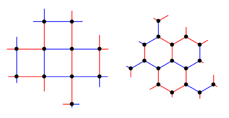
We are interested in thermodynamic properties of various spin-1/2 models on the square and honeycomb lattices (see Fig. 1). In the absence of disorder, and for nearest neighbor interactions, those models do not exhibit frustration on either lattice, which are both bipartite. While the thermodynamic properties of the various models studied here are qualitatively similar on both lattice geometries, there are significant quantitative differences, e.g., in the critical temperatures for the onset of quasi-long-range order.Sykes and Fisher (1962) These differences have their origin in the different coordination number in both lattices, with the honeycomb lattice having the smallest one. Hence, not surprisingly, for the spin-1/2 antiferromagnetic Heisenberg model, the staggered magnetization is significantly suppressed on the honeycomb lattice as compared with the square lattice.Weihong et al. (1991) Disorder, on the other hand, leads to frustration on both lattices, and to a qualitative change of the intermediate to low temperature properties with respect to the clean systems. Frustration can be easily identified by trying to assign spins to the various sites in Fig. 1 to minimize the energy. If one takes the Ising Hamiltonian discussed below, one finds that for the overwhelming majority of disorder realizations there is no single spin configuration that minimizes the energy on all bonds.
We should stress that both for the clean and disordered cases, we expect quantum fluctuations to strongly modify the results for the spin-1/2 XY and Heisenberg models from their classical counterparts (see, e.g., Ref. Di Ciolo et al., 2014 for examples of the effects of quantum fluctuations in frustrated spin-1/2 XY and Heisenberg models on the honeycomb lattice). Our focus in this work is on systems with bimodal random-bond disorder, where the nearest-neighbor coupling between the spins takes values with equal probability.
II.1 Ising model
The Hamiltonian for the spin-1/2 Ising model can be written as
| (1) |
where is the spin at site-, and the sum is over nearest neighbors. In the absence of disorder ( for all ), Eq. (1) has served as the quintessential model for magnetism and was solved exactly on a 2D square lattice by Onsager.Onsager (1944) In the presence of continuous disorder, the Hamiltonian in Eq. (1), commonly known as the Edwards-Anderson model,Edwards and Anderson (1975) has also become a widely studied model for spin-glasses.
The Ising model has a discrete symmetry, i.e., the transformation for all leaves the Hamiltonian invariant. This symmetry can be spontaneously broken at sufficiently low temperatures to create an ordered phase. For , the critical temperature is given by for the square lattice, and for the honeycomb lattice, and is the same for the ferro- and antiferromagnetic cases.Sykes and Fisher (1962) The latter is because, for bipartite lattices, a unitary transformation relates both models. This can be easily seen by rewriting the Hamiltonian in Eq. (1) as , where and are the two sub-lattice indices. One can then go from , i.e., between the ferro- and antiferromagnetic models, via the transformation: and .
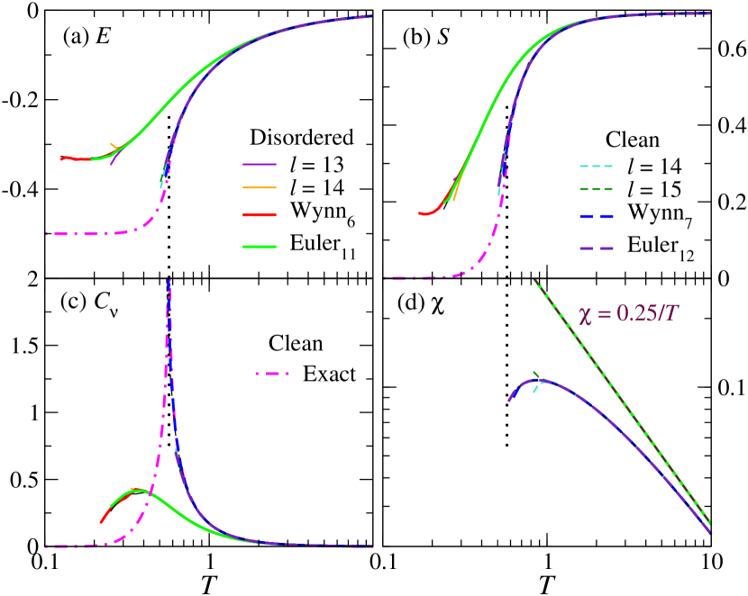
The specific heat of the clean model diverges at the critical temperature for both the square and the honeycomb lattices. Equivalently, the derivative of the energy diverges at the critical temperature but the energy remains finite throughout. For the antiferromagnetic model, the susceptibility is known to be finite everywhere, with an infinite slope at the critical temperature. The maximum value of the susceptibility occurs at and for the square and honeycomb models respectively,Fisher (1959); Sykes and Fisher (1962) i.e., above the critical temperature. Our results for the clean systems are consistent with these. However, we cannot study the critical phase or the properties of the system very close to criticality (see Figs. 3 and 4).
The Ising model with bimodal disorder has been extensively studied in the past.Cho and Fisher (1997); Blackman et al. (1998); Hartmann and Young (2001); Gruzberg et al. (2001); Amoruso and Hartmann (2004); Lukic et al. (2004); Katzgraber and Lee (2005); Katzgraber et al. (2007); Atisattapong and Poulter (2009); Thomas et al. (2011); Parisen Toldin et al. (2011) It is reasonably well established that no glassy phase exists for .Hartmann and Young (2001); Gruzberg et al. (2001) It has, however, been established that a glassy phase appears at zero temperature in this model.Thomas et al. (2011) At finite temperature, our results for this case are described in Sec. IV.1.
II.2 XY Model
The spin-1/2 XY model can be written as
| (2) |
where are spin operators at site , proportional to the Pauli matrices. We consider only the isotropic case, where the model has a continuous rotation symmetry in the plane. The presence of a continuous symmetry precludes, via the Mermin-Wagner theorem,Mermin and Wagner (1966) a finite-temperature phase-transition involving the breaking of this continuous symmetry from occurring. For dimensions, the fluctuations in any putative ordered phase appearing from breaking a continuous symmetry grow with system size for finite temperatures, destroying any order (see e.g., Ref. Altland and Simons, 2006). Hence, this model has an ordered phase only at .
However, in 2D there can still be a finite temperature Berezinskii-Kosterlitz-Thouless (BKT) transitionBerezinskiǐ (1972); Kosterlitz and Thouless (1973) below which the system exhibits quasi-long-range spin order. The critical temperature for the BKT transition in the spin-1/2 XY model in the square lattice is .Harada and Kawashima (1998); Carrasquilla and Rigol (2012) We should stress that both classicalBerezinskiǐ (1971) and quantum models with continuous symmetries in 2D can exhibit this kind of behavior.Fröhlich and Spencer (1981) We should also mention that most studies in the literature report results for the ferromagnetic XY model (). However, like for the Ising model, in the square and honeycomb lattice a unitary transformation relates the ferro- and antiferromagnetic models and the critical temperature is the same in both. Our calculations for the susceptibility of the clean case on the square lattice converge down to temperatures of , which is compatible with the onset of quasi-long-range order for .Harada and Kawashima (1998); Carrasquilla and Rigol (2012)
II.3 Heisenberg model
The spin-1/2 Heisenberg model, also known as the XXX model, can be written as
| (3) |
where , and are spin operators at site , proportional to the Pauli matrices. The Heisenberg model has an symmetry, the highest of the three models considered in this work. The ground state in the clean case () is an ordered ferromagnet or antiferromagnet depending on the sign of the coupling constant . Like for the XY model, long-range order only occurs at zero temperature. However, in contrast to the XY model, the 2D Heisenberg model does not develop quasi-long-range order at finite temperature. This is due to the fact that the internal symmetry group, [] for the quantum (classical) Heisenberg model, is non-Abelian, as opposed to the XY model which has an Abelian symmetry group, [] for the quantum (classical) cases. Vortices or point-defects, which are responsible for the BKT transition,Kosterlitz and Thouless (1973) occur only in the latter case.Kenna (2005) Furthermore, in 2D, models with or models with , i.e., with non-Abelian symmetry groups, can be shown via perturbation theory to be asymptotically free, which for spin models translates to a renormalization group flow towards paramagnetism.Gross and Wilczek (1973); Gross (1999)
The results for the clean system presented here for the square lattice are nearly identical to the spin-1/2 results presented in Ref. Cuccoli et al., 1997, which also compares with other known results.
III Numerical Linked Cluster Expansions
Numerical linked cluster expansions (NLCEs) are a computational technique that can be used to calculate extensive properties (per lattice site) of translationally invariant lattice systems. NLCEs, which are based on linked cluster expansions,Domb (1960a, b); Sykes et al. (1966) were introduced in Ref. Rigol et al., 2006, where it was shown that the results obtained for thermodynamic properties were exact in the thermodynamic limit for systems with a finite correlation length. Furthermore, results could be obtained at significantly lower temperatures as compared to high-temperature expansions for models that develop long-range order at zero temperature. In several subsequent works, NLCEs have been shown to be a powerful computational technique for determining not only thermodynamic properties of a variety of lattice models,Rigol et al. (2007a, b); Khatami and Rigol (2011a, b); Tang et al. (2012, 2013) but also for studying thermalization (or the lack thereof) at long times after a quench in isolated quantum systems.Rigol (2014a); Wouters et al. (2014); Rigol (2014b); Tang et al. For completeness, we provide a brief description of NLCEs. Details of how to implement them can be found in Ref. Tang et al., 2013.
In NLCEs, the expectation value of an extensive observable, per-site, in a translationally invariant system can be calculated as a sum over contributions from all clusters of different sizes that can be embedded on the lattice
| (4) |
where is a combinatorial factor equal to the number of ways that a particular cluster can be embedded on that lattice. is the weight of cluster for the given observable, which is calculated via the inclusion-exclusion principle
| (5) |
is the expectation value of the observable on the specific cluster . Within NLCEs, is calculated using full exact diagonalization. The expansion is carried out order by order, i.e., by first considering clusters with one-site, then two-sites, and so on. Beyond the bare sum in Eq. (4), several resummation schemes exist that accelerate the convergence of the expansion.Rigol et al. (2007a) Here we will report results from Wynn and Euler resummation techniques whenever they allow us to extend the convergence of the results to lower temperatures.Rigol et al. (2007a)
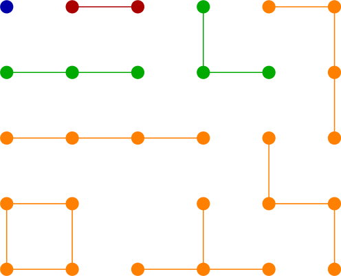
Examples of clusters up to fourth order in the site-based NLCE used here on the square lattice are shown in Fig. 2. At third order, although there are two geometrically different clusters, they are topologically identical. They have the same Hamiltonian for the models with nearest interactions we consider here. At fourth order, there are three clusters (including the one with the four sites on a line) that again have the same Hamiltonian for the models considered here. However, two topologically new clusters appear, namely, the closed loop and the “”. They have to be individually diagonalized. From the fourth order and beyond the number of distinct topological clusters increases rapidly (exponentially with the number of sites), making the calculations increasingly costly. References Rigol et al., 2007a; Tang et al., 2013 provide details on the various topological clusters on the square and honeycomb lattices, respectively, as well as the number of such clusters as a function of the order of the expansion.
Recently, in Ref. Tang et al., , it was shown that NLCEs can also be used to study systems with disorder. As described above, NLCEs can only be used for translationally invariant systems. A priori, disorder breaks translational invariance. However, we are only interested in disorder averaged physical quantities. If we take a disorder average over all possible disorder configurations in models with bimodal disorder, we restore translational invariance and the equivalent of Eq. (4) reads
| (6) |
where the overline denotes the disorder average. The disorder average of the weights is in turn given by
| (7) |
In other words, the disorder average can be carried out order by order for each observable. The calculations then proceed as for the translationally invariant system if one replaces by .
The computations in the presence of disorder are much more challenging than for translationally invariant systems because of the additional average over all possible disorder realizations. For example, the largest clusters we consider here for the quantum models in the square lattice have 13 sites. At this order, there are a total of connected clusters, of which 5,450 are topologically distinct.Rigol et al. (2007a) Each of these has to be fully diagonalized for the disorder configurations corresponding to the bonds in the cluster. This has to, of course, be carried out for all lower orders as well, each with a different set of topologically distinct clusters and disorder configurations. For the clean systems, we report results for cluster with up to 15 sites for the square lattice. In that case one has to diagonalize 42,192 topologically distinct clusters with 15 sites.
NLCE calculations fail to converge when correlations in the thermodynamic limit extend beyond the largest clusters considered. Therefore, NLCEs cannot be used to calculate observables in phases with long-range order unless one tailors the expansion to account for those.Khatami et al. (2011) Since disorder usually shortens correlations at low temperatures, NLCEs are particularly useful to study quantum disordered systems, despite the increase of computational cost because of the disorder average. It will become apparent when we discuss our results for the various thermodynamic properties of interest in this work, that NLCEs converge to lower temperatures in disordered systems when compared to clean systems. As mentioned before, quantum Monte Carlo simulations in the presence of disorder are severely limited by the sign problem.
IV Results
In this section, we discuss the results of our NLCE based study of the three spin models described in Sec. II on the square and honeycomb lattices. In what follows, we set as the energy scale. For each model and lattice geometry, we report the energy (), entropy (), specific heat (), and uniform susceptibility for the magnetization along the -axis () as a function of temperature. These quantities are defined as
| (8) |
where the overline denotes a disorder average, the angle brackets denote the thermal expectation value in the grand-canonical ensemble (at zero chemical potential), is the number of sites, and is the temperature. As mentioned earlier, the disorder average is carried out over all disorder configurations at each order in the NLCE. In all cases, the disorder averaged results are compared with the ones in clean systems.
For all observables, we report bare NLCE results for the highest two orders of our site-based NLCE expansion, which are determined by the number of sites in the largest clusters studied. Namely, we report the results from Eq. (6) when the contributions of all clusters with up to sites are added, where takes the two largest values in our calculations for each model in each lattice geometry. We also report results using two different resummation schemes, indicated as Wynnn and Eulern. The subscript denotes the order of the resummation process (see Ref. Rigol et al., 2007a for details). The resummation schemes allow us to access significantly lower temperatures than the bare results in some cases as indicated below.
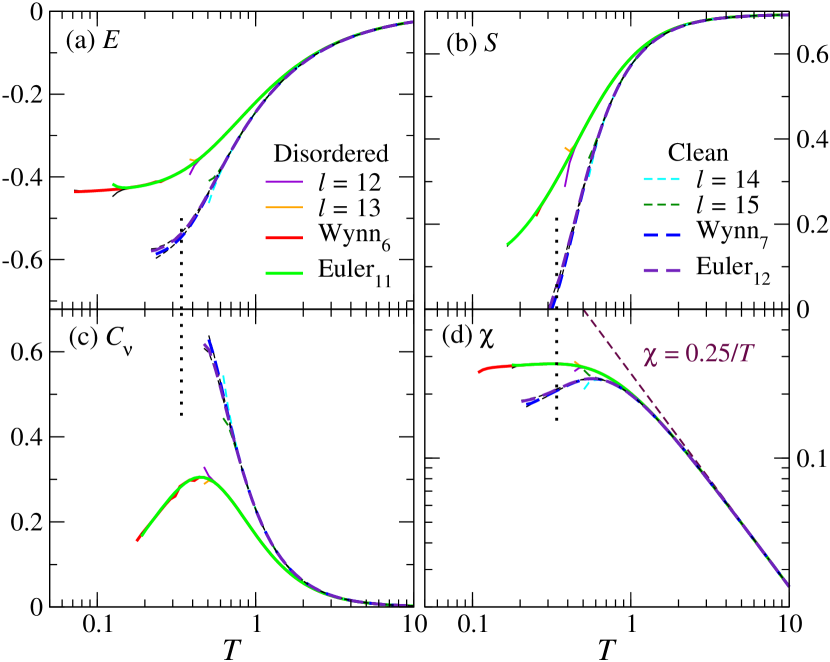
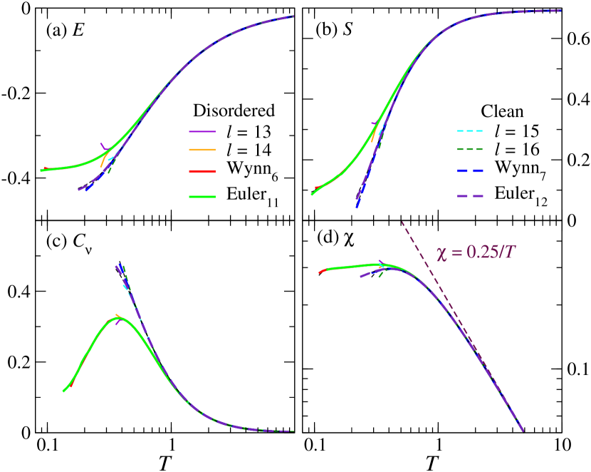
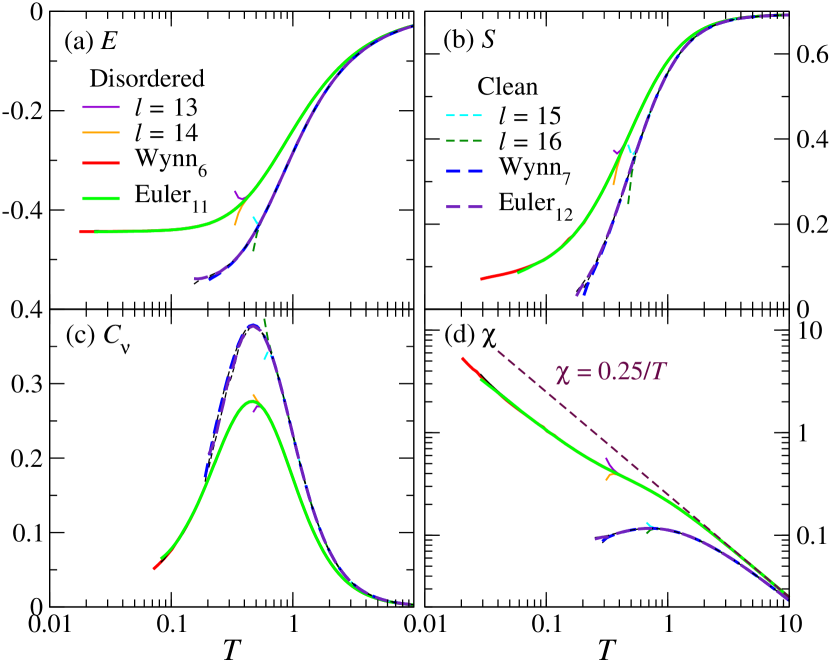
Before discussing each model and observable in detail, we review a few general observations for completeness and pedagogy. In all models and observables discussed here, the numerical results at intermediate to high temperatures in the presence of disorder are close to those of the corresponding clean system. Whereas this is obvious for temperatures so high that the first order correction to the infinite temperature result is negligibly small, we notice from our results in Figs. 3–8 that the observables in clean and disordered models are indistinguishable for temperatures as low as (barring the susceptibility).
In order to show why this is so, we expand the partition function for small inverse temperature , . The models we consider have only nearest-neighbor coupling, i.e., , where we have included a magnetic field as a source to calculate the uniform susceptibility in the -direction. The most general two-site Hamiltonian that describes all models of interest here is given by , which becomes the Ising model for , the XY model for , and the Heisenberg model for . With this in mind, to first order in , the high temperature expansion for can be written as , where is the number of lattice sites. Note first that (the Pauli matrices are traceless), and second, that , so that the linear correction vanishes. Therefore, to first order in , the clean and the disordered system have the same partition function. This is true regardless of the type of disorder.
To second order, after expanding , we have
| (9) |
Let us treat the above terms one by one. In the first term, for , the trace is identically zero as shown above. For the case when say , but , we effectively have a new Hamiltonian for three neighboring spins. It is easy to verify explicitly that this trace also vanishes. The only possibility left for a nonvanishing contribution is . The trace of second term in the brackets is nonzero only for . In the third term, again for , the trace is zero. For, say , considering only the diagonal elements of the matrix, , we see that the trace vanishes. Taking these into account, and writing to , we have
| (10) |
For both, the clean system and the system with bimodal disorder, . We therefore get,
| (11) |
where is the Hamiltonian for a two-site system and the subscript “2” on the trace indicates a trace over the Fock space of a two-site system. The disorder average does not change the above expression, and therefore to this order, the clean and the disordered systems behave identically. The energy, for instance, is given to this order by , the specific heat is , and the uniform susceptibility is .
In fact, it is straightforward to check that the partition function in the clean and disordered systems remains the same at , except for terms proportional to . In other words, the energy, entropy, and specific heat are the same for clean and disordered systems up to third order in , but the uniform susceptibility deviates. The following expression can be derived along the lines of Eqs. (9)–(11) for the third order correction to the partition function:
| (12) |
There is no sum over , which represent the two sites in a 2-site system. For the clean model one just needs to replace with in the above formula, while for the disordered one, the disorder average produces two terms for (which cancel each other, implying that disorder extends the paramagnetic behavior in the susceptibility to lower temperatures). One can the see that for , all thermodynamic quantities studied here, except the susceptibility, are identical in the clean and disordered cases up to . One can further verify that this changes at fourth order, where differences emerge between clean and disordered systems. An example of a term that makes a difference at fourth order is a square loop with four sites and four bonds (see Fig. 2). Even in the Ising case, the Hamiltonian has a nonzero trace with a product of four different .
We should stress that, in all models studied here in the presence of disorder, we find that there is a significant amount of residual entropy (when comparing with the clean systems) at the lowest temperatures we are able to access with NLCEs. This is a clear indication of the lack of order at those temperatures. The behavior of the entropy, coupled with a saturation of the energy observed at the lowest temperatures accessible to us, confirms that there are many energy levels close to each other at low energies. This is the hallmark of frustration.
IV.1 Ising model
Figures 3 and 4 show the energy (a), entropy (b), specific heat (c), and uniform susceptibility (d) for the disordered spin-1/2 Ising model on the square and honeycomb lattices, respectively. For the square lattice, we also plot the exact results for , , and for the clean model.Onsager (1944); Huang (1987) Several approximate analytic estimates exist for the susceptibility, but there is no closed form expression for all temperatures.
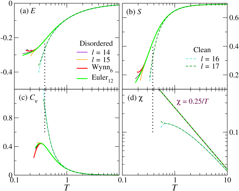
Figures 3(a) and 4(a) show that, as mentioned before, a generic feature in the presence of disorder is that the energy tends to plateau at the lowest temperatures accessible to us. In that regime, the entropy is significantly higher than in the clean systems [Figs. 3(b) and 4(b)]. Distinct to the Ising models, the sharp divergence in the specific heat in the clean case [see Figs. 3(c) and 4(c)], which indicates the phase transition, is replaced by what appears to be smooth peak in the presence of disorder. The maximum of that peak appears at temperatures lower than the critical temperature in the clean case. At higher temperatures, Eq. (11) gives results that agree for , , and down to . We note that NLCE results for the disordered model are well converged down to to 0.3, while the NLCE results for the clean model converge to temperatures that are close to , and agree with the analytic results in the disordered phase.
Results for the uniform susceptibility in Figs. 3(d) and 4(d) show that this quantity behaves very differently in the clean and disordered systems. In the disordered case it exhibits a behavior at all temperatures, both on the square and honeycomb lattices. An order by order linked cluster expansion reveals that the only nonvanishing contribution to the susceptibility in the disordered case comes from the single-site system, and is trivially proportional to . All higher order contributions vanish. We show this for the first few orders of the NLCE on the square lattice. Below are the expressions for the disorder averaged for the clusters with one, two, and three sites shown in Fig. 2.
| (13) |
The uniform susceptibility can be obtained from evaluated at . We get for the above three orders,
| (14) |
Already, one can see that no new contributions appear at the higher orders. To confirm this, we calculate the weights of the three clusters (see Ref. Rigol et al., 2007a for details about multiplicities, etc.):
| (15) |
Indeed, only the single-site cluster contributes. One can check this at higher orders, and for the honeycomb lattice as well. This is not the case for the XY and Heisenberg models discussed below.
Earlier studies for the Ising model with bimodal disorder on the square lattice found a low-temperature scaling of the specific heat (i.e., the exponent in a power law fit of the low-temperature specific heat, ) that is different from the model with continuous disorder.Katzgraber et al. (2007) At even lower temperatures, a crossover in the scaling behavior of has been reported.Thomas et al. (2011) Unfortunately, our results do not converge at low enough temperatures to observe such power laws. However, for , our results are consistent with those in other studiesKatzgraber et al. (2007); Thomas et al. (2011) (since we consider , our temperatures are lower by a factor of four from those studies, which took ).
IV.2 XY model
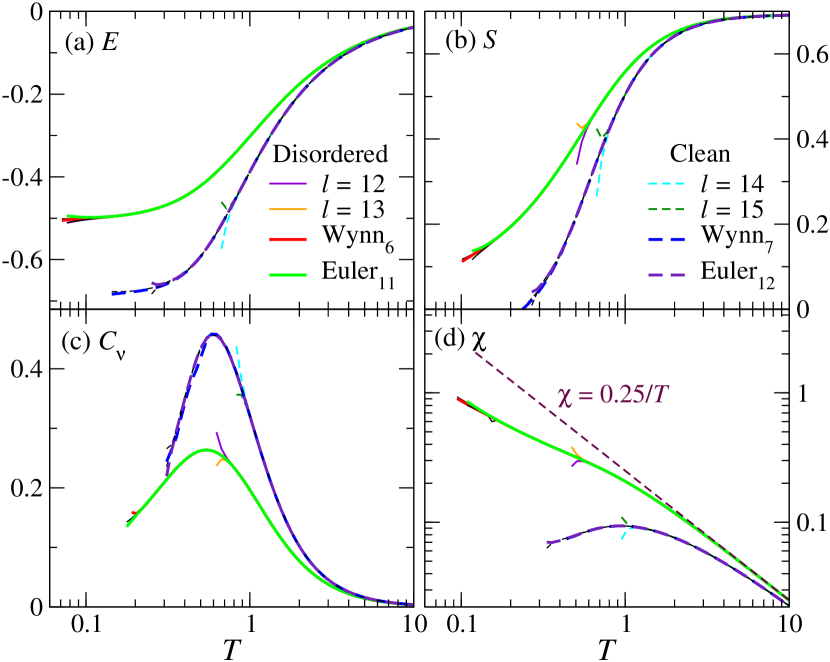
Figures 5 and 6 show results for the spin-1/2 XY model on the square and honeycomb lattice, respectively. The results for all quantities are well converged down to about to 0.2. Figures 5(a),(b) and 6(a),(b) show that the behavior of energy and the entropy is qualitatively similar to the one observed in the Ising model. However, the results for the XY model in the presence of disorder converge at lower temperature than those for the Ising model. For the XY model, the specific heat in the presence of disorder exhibits a peak that is well resolved by our NLCE [Figs. 5(c) and 6(c)]. We note that the energy, entropy, and specific heat follow the second order result in Eq. (11) for in the square lattice and in the honeycomb lattice.
Interestingly, Figs. 5(d) and 6(d) show that in the XY model the uniform (-)susceptibility in the presence of disorder exhibits a plateau for low temperatures. This is qualitatively different from the behavior observed for the Ising model. The fact that the response to an external magnetic field in the -direction is independent of temperature for low temperatures shows that increasing temperature does not increase the disorder in the spin correlations in the -direction.
We should add that the classical XY model has been studied in the presence of Gaussian-random dilutionDeng and Gu (2014) and bimodal dilutionSurungan and Okabe (2005) of ferromagnetic bonds. In these works, the BKT transition was seen to slowly disappear as the dilution was increased. Here we only have considered the fully disordered case, i.e., an equal distribution of ferro- and antiferromagnetic bonds, so we do not expect that any remnants of the BKT phase are present in our calculations.
IV.3 Heisenberg model
Figures 7 and 8 show results for the spin-1/2 Heisenberg model on the square and honeycomb lattices, respectively. In Figs. 7(a) and 8(a), one can see that the plateau in the energy at low temperatures is the clearest of all models studied in this work. The onset of this plateau occurs at for both models. Remarkably, in the honeycomb geometry, the energy in the presence of disorder converges down to . The entropy [Figs. 7(b) and 8(b)] behaves similarly to the entropy in the XY model, but also converges to very low temperatures ( to 0.04) in the honeycomb geometry. Like for the XY model, the specific heat exhibits a clear peak in the presence of disorder. The temperature at which the maximum of that peak occurs is very close (but slightly larger) to the one in the clean model.
In contrast to the XY model, the uniform susceptibility in the presence of disorder increases rapidly with decreasing temperature at the lowest temperatures accessible to us. The susceptibility therefore behaves qualitatively similar to the Ising model. It is worth emphasizing that our results for all observables in the honeycomb lattice appear to converge at temperatures significantly below , and quite close to for the energy, entropy, and uniform susceptibility.
Our calculations for the Heisenberg model reach lower temperatures and access regimes beyond what has been possible with quantum Monte Carlo simulations. For example, Ref. Sandvik, 1994 studied the case of diluting an antiferromagnetic model with ferromagnetic bonds of varying concentration. The results presented there did not reach the equal probability case discussed here because of the sign problem. For lower concentrations of ferromagnetic bonds (below 30%), the calculations were still limited to temperatures above .
V Summary
We have used numerical linked cluster expansions to study thermodynamic properties of spin models with bimodal () bond disorder. The results reported are in the thermodynamic limit at temperatures for which they are well converged.
We have unveiled various interesting effects of disorder in spin-1/2 Ising, XY, and Heisenberg models. For all models we find that disorder leads to a saturation of the energy at the lowest temperatures accessible to us, in a regime where the entropy is higher than in clean systems. This makes apparent that there are many low lying energy states. For the disordered classical Ising model, on both the square and the honeycomb lattice, the divergence of the specific heat in the clean case is replaced by a peak, and the uniform susceptibility follows an inverse temperature law for all temperatures in the presence of disorder. This was explicitly verified order by order. In the Heisenberg model, we also find that the susceptibility increases with decreasing temperature for all temperatures accessible to us in the presence of disorder. In the XY model, on the other hand, we find that the susceptibility exhibits a plateau at low temperatures. On both the XY and Heisenberg models, our NLCE calculations were able to resolve a peak in the specific heat.
VI Acknowledgments
We acknowledge support from the National Science Foundation (NSF), Grant No. OCI-0904597, and the U.S. Office of Naval Research.
References
- Anderson (1958) P. W. Anderson, Phys. Rev. 109, 1492 (1958).
- Binder and Young (1986) K. Binder and A. P. Young, Rev. Mod. Phys. 58, 801 (1986).
- Weissman (1993) M. Weissman, Rev. Mod. Phys. 65, 829 (1993).
- Katzgraber et al. (2007) H. G. Katzgraber, L. W. Lee, and I. A. Campbell, Phys. Rev. B 75, 014412 (2007).
- Parisen Toldin et al. (2011) F. Parisen Toldin, A. Pelissetto, and E. Vicari, Phys. Rev. E 84, 051116 (2011).
- Thomas and Middleton (2013) C. Thomas and A. Middleton, Phys. Rev. E 87, 043303 (2013).
- Thomas et al. (2011) C. Thomas, D. Huse, and A. Middleton, Phys. Rev. Lett. 107, 047203 (2011).
- Henelius and Sandvik (2000) P. Henelius and A. Sandvik, Phys. Rev. B 62, 1102 (2000).
- Troyer and Wiese (2005) M. Troyer and U.-J. Wiese, Phys. Rev. Lett. 94, 170201 (2005).
- (10) B. Tang, D. Iyer, and M. Rigol, arXiv:1411.0699 .
- Rigol (2014a) M. Rigol, Phys. Rev. Lett. 112, 170601 (2014a).
- Wouters et al. (2014) B. Wouters, J. De Nardis, M. Brockmann, D. Fioretto, M. Rigol, and J.-S. Caux, Phys. Rev. Lett. 113, 117202 (2014).
- Rigol (2014b) M. Rigol, Phys. Rev. E 90, 031301(R) (2014b).
- Sykes and Fisher (1962) M. Sykes and M. E. Fisher, Physica 28, 919 (1962).
- Weihong et al. (1991) Z. Weihong, J. Oitmaa, and C. Hamer, Phys. Rev. B 44, 11869 (1991).
- Di Ciolo et al. (2014) A. Di Ciolo, J. Carrasquilla, F. Becca, M. Rigol, and V. Galitski, Phys. Rev. B 89, 094413 (2014).
- Onsager (1944) L. Onsager, Phys. Rev. 65, 117 (1944).
- Edwards and Anderson (1975) S. F. Edwards and P. W. Anderson, J. Phys. F: Met. Phys. 5, 965 (1975).
- Fisher (1959) M. E. Fisher, Physica 25, 521 (1959).
- Cho and Fisher (1997) S. Cho and M. P. A. Fisher, Phys. Rev. B 55, 1025 (1997).
- Blackman et al. (1998) J. A. Blackman, J. R. Gonçalves, and J. Poulter, Phys. Rev. E 58, 1502 (1998).
- Hartmann and Young (2001) A. K. Hartmann and A. P. Young, Phys. Rev. B 64, 180404 (2001).
- Gruzberg et al. (2001) I. Gruzberg, N. Read, and A. Ludwig, Phys. Rev. B 63, 104422 (2001).
- Amoruso and Hartmann (2004) C. Amoruso and A. K. Hartmann, Phys. Rev. B 70, 134425 (2004).
- Lukic et al. (2004) J. Lukic, A. Galluccio, E. Marinari, O. C. Martin, and G. Rinaldi, Phys. Rev. Lett. 92, 117202 (2004).
- Katzgraber and Lee (2005) H. G. Katzgraber and L. W. Lee, Phys. Rev. B 71, 134404 (2005).
- Atisattapong and Poulter (2009) W. Atisattapong and J. Poulter, New Journal of Physics 11, 063039 (2009).
- Mermin and Wagner (1966) N. D. Mermin and H. Wagner, Phys. Rev. Lett. 17, 1133 (1966).
- Altland and Simons (2006) A. Altland and B. Simons, Condensed Matter Field Theory (Cambridge Univ. Press, 2006).
- Berezinskiǐ (1972) V. L. Berezinskiǐ, Sov. JETP 34, 610 (1972).
- Kosterlitz and Thouless (1973) J. M. Kosterlitz and D. J. Thouless, J. Phys. C: Solid State Phys. 6, 1181 (1973).
- Harada and Kawashima (1998) K. Harada and N. Kawashima, J. Phys. Soc. Jpn. 67, 2768 (1998).
- Carrasquilla and Rigol (2012) J. Carrasquilla and M. Rigol, Phys. Rev. A 86, 043629 (2012).
- Berezinskiǐ (1971) V. L. Berezinskiǐ, Sov. JETP 32, 493 (1971).
- Fröhlich and Spencer (1981) J. Fröhlich and T. Spencer, Comm. Math. Phys. 81, 527 (1981).
- Kenna (2005) R. Kenna, arXiv:cond-mat/0512356 (2005).
- Gross and Wilczek (1973) D. Gross and F. Wilczek, Phys. Rev. Lett. 30, 1343 (1973).
- Gross (1999) D. J. Gross, Nucl. Phys. B - Proc. Suppl. 74, 426 (1999), {QCD} 98.
- Cuccoli et al. (1997) A. Cuccoli, V. Tognetti, R. Vaia, and P. Verrucchi, Phys. Rev. B 56, 14456 (1997).
- Domb (1960a) C. Domb, Advances in Physics 9, 149 (1960a), http://dx.doi.org/10.1080/00018736000101189 .
- Domb (1960b) C. Domb, Advances in Physics 9, 245 (1960b), http://dx.doi.org/10.1080/00018736000101199 .
- Sykes et al. (1966) M. F. Sykes, J. W. Essam, B. R. Heap, and B. J. Hiley, Journal of Mathematical Physics 7, 1557 (1966).
- Rigol et al. (2006) M. Rigol, T. Bryant, and R. R. P. Singh, Phys. Rev. Lett. 97, 187202 (2006).
- Rigol et al. (2007a) M. Rigol, T. Bryant, and R. R. P. Singh, Phys. Rev. E 75, 061118 (2007a).
- Rigol et al. (2007b) M. Rigol, T. Bryant, and R. R. P. Singh, Phys. Rev. E 75, 061119 (2007b).
- Khatami and Rigol (2011a) E. Khatami and M. Rigol, Phys. Rev. B 83, 134431 (2011a).
- Khatami and Rigol (2011b) E. Khatami and M. Rigol, Phys. Rev. A 84, 053611 (2011b).
- Tang et al. (2012) B. Tang, T. Paiva, E. Khatami, and M. Rigol, Phys. Rev. Lett. 109, 205301 (2012).
- Tang et al. (2013) B. Tang, T. Paiva, E. Khatami, and M. Rigol, Phys. Rev. B 88, 125127 (2013).
- Tang et al. (2013) B. Tang, E. Khatami, and M. Rigol, Comput. Phys. Commun. 184, 557 (2013).
- Khatami et al. (2011) E. Khatami, R. R. P. Singh, and M. Rigol, Phys. Rev. B 84, 224411 (2011).
- Huang (1987) K. Huang, Statistical mechanics (Wiley, New York, 1987).
- Deng and Gu (2014) Y.-B. Deng and Q. Gu, Chin. Phys. Lett. 31, 020504 (2014).
- Surungan and Okabe (2005) T. Surungan and Y. Okabe, Phys. Rev. B 71, 184438 (2005).
- Sandvik (1994) A. W. Sandvik, Phys. Rev. B 50, 15803 (1994).