Difference Target Propagation
Abstract
Back-propagation has been the workhorse of recent successes of deep learning but it relies on infinitesimal effects (partial derivatives) in order to perform credit assignment. This could become a serious issue as one considers deeper and more non-linear functions, e.g., consider the extreme case of non-linearity where the relation between parameters and cost is actually discrete. Inspired by the biological implausibility of back-propagation, a few approaches have been proposed in the past that could play a similar credit assignment role. In this spirit, we explore a novel approach to credit assignment in deep networks that we call target propagation. The main idea is to compute targets rather than gradients, at each layer. Like gradients, they are propagated backwards. In a way that is related but different from previously proposed proxies for back-propagation which rely on a backwards network with symmetric weights, target propagation relies on auto-encoders at each layer. Unlike back-propagation, it can be applied even when units exchange stochastic bits rather than real numbers. We show that a linear correction for the imperfectness of the auto-encoders, called difference target propagation, is very effective to make target propagation actually work, leading to results comparable to back-propagation for deep networks with discrete and continuous units and denoising auto-encoders and achieving state of the art for stochastic networks. 111This paper was accepted in ECML/PKDD 2015. Please cite like following : Dong-Hyun Lee, Saizheng Zhang, Asja Fischer and Yoshua Bengio, Difference Target Propagation, in Machine Learning and Knowledge Discovery in Databases, pages 498-515, Springer International Publishing, 2015
1 Introduction
Recently, deep neural networks have achieved great success in hard AI tasks [2, 11, 13, 18], mostly relying on back-propagation as the main way of performing credit assignment over the different sets of parameters associated with each layer of a deep net. Back-propagation exploits the chain rule of derivatives in order to convert a loss gradient on the activations over layer (or time , for recurrent nets) into a loss gradient on the activations over layer (respectively, time ). However, as we consider deeper networks– e.g., consider the recent best ImageNet competition entrants [19] with 19 or 22 layers – longer-term dependencies, or stronger non-linearities, the composition of many non-linear operations becomes more strongly non-linear. To make this concrete, consider the composition of many hyperbolic tangent units. In general, this means that derivatives obtained by back-propagation are becoming either very small (most of the time) or very large (in a few places). In the extreme (very deep computations), one would get discrete functions, whose derivatives are 0 almost everywhere, and infinite where the function changes discretely. Clearly, back-propagation would fail in that regime. In addition, from the point of view of low-energy hardware implementation, the ability to train deep networks whose units only communicate via bits would also be interesting.
This limitation of back-propagation to working with precise derivatives and smooth networks is the main machine learning motivation for this paper’s exploration into an alternative principle for credit assignment in deep networks. Another motivation arises from the lack of biological plausibility of back-propagation, for the following reasons: (1) the back-propagation computation is purely linear, whereas biological neurons interleave linear and non-linear operations, (2) if the feedback paths were used to propagate credit assignment by back-propagation, they would need precise knowledge of the derivatives of the non-linearities at the operating point used in the corresponding feedforward computation, (3) similarly, these feedback paths would have to use exact symmetric weights (with the same connectivity, transposed) of the feedforward connections, (4) real neurons communicate by (possibly stochastic) binary values (spikes), (5) the computation would have to be precisely clocked to alternate between feedforward and back-propagation phases, and (6) it is not clear where the output targets would come from.
The main idea of target propagation is to associate with each feedforward unit’s activation value a target value rather than a loss gradient. The target value is meant to be close to the activation value while being likely to have provided a smaller loss (if that value had been obtained in the feedforward phase). In the limit where the target is very close to the feedforward value, target propagation should behave like back-propagation. This link was nicely made in [15, 16], which introduced the idea of target propagation and connected it to back-propagation via a Lagrange multipliers formulation (where the constraints require the output of one layer to equal the input of the next layer). A similar idea was recently proposed where the constraints are relaxed into penalties, yielding a different (iterative) way to optimize deep networks [9]. Once a good target is computed, a layer-local training criterion can be defined to update each layer separately, e.g., via the delta-rule (gradient descent update with respect to the cross-entropy loss).
By its nature, target propagation can in principle handle stronger (and even discrete) non-linearities, and it deals with biological plausibility issues (1), (2), (3) and (4) described above. Extensions of the precise scheme proposed here could handle (5) and (6) as well, but this is left for future work.
In this paper, we describe how the general idea of target propagation by using auto-encoders to assign targets to each layer (as introduced in an earlier technical report [4]) can be employed for supervised training of deep neural networks (section 2.1 and 2.2). We continue by introducing a linear correction for the imperfectness of the auto-encoders (2.3) leading to robust training in practice. Furthermore, we show how the same principles can be applied to replace back-propagation in the training of auto-encoders (section 2.4). In section 3 we provide several experimental results on rather deep neural networks as well as discrete and stochastic networks and auto-encoders. The results show that the proposed form of target propagation is comparable to back-propagation with RMSprop [21] - a very popular setting to train deep networks nowadays- and achieves state of the art for training stochastic neural nets on MNIST.
2 Target Propagation
Although many variants of the general principle of target propagation can be devised, this paper focuses on a specific approach, which is based on the ideas presented in an earlier technical report [4] and is described in the following.
2.1 Formulating Targets
Let us consider an ordinary (supervised) deep network learning process, where the training data is drawn from an unknown data distribution . The network structure is defined by
| (1) |
where is the state of the -th hidden layer (where corresponds to the output of the network and ) and is the -th layer feed-forward mapping, defined by a non-linear activation function (e.g. the hyperbolic tangents or the sigmoid function) and the weights of the -th layer. Here, for simplicity of notation, the bias term of the -th layer is included in . We refer to the subset of network parameters defining the mapping between the -th and the -th layer () as . Using this notion, we can write as a function of depending on parameters , that is we can write .
Given a sample , let be an arbitrary global loss function measuring the appropriateness of the network output for the target , e.g. the MSE or cross-entropy for binomial random variables. Then, the training objective corresponds to adapting the network parameters so as to minimize the expected global loss under the data distribution . For we can write
| (2) |
to emphasize the dependency of the loss on the state of the -th layer.
Training a network with back-propagation corresponds to propagating error signals through the network to calculate the derivatives of the global loss with respect to the parameters of each layer. Thus, the error signals indicate how the parameters of the network should be updated to decrease the expected loss. However, in very deep networks with strong non-linearities, error propagation could become useless in lower layers due to exploding or vanishing gradients, as explained above.
To avoid this problems, the basic idea of target propagation is to assign to each a nearby value which (hopefully) leads to a lower global loss, that is which has the objective to fulfill
| (3) |
Such a is called a target for the -th layer.
Given a target we now would like to change the network parameters to make move a small step towards , since – if the path leading from to is smooth enough – we would expect to yield a decrease of the global loss. To obtain an update direction for based on we can define a layer-local target loss , for example by using the MSE
| (4) |
Then, can be updated locally within its layer via stochastic gradient descent, where is considered as a constant with respect to . That is
| (5) |
where is a layer-specific learning rate.
Note, that in this context, derivatives can be used without difficulty, because they correspond to computations performed inside a single layer. Whereas, the problems with the severe non-linearities observed for back-propagation arise when the chain rule is applied through many layers. This motivates target propagation methods to serve as alternative credit assignment in the context of a composition of many non-linearities.
However, it is not directly clear how to compute a target that guarantees a decrease of the global loss (that is how to compute a for which equation (3) holds) or that at least leads to a decrease of the local loss of the next layer, that is
| (6) |
Proposing and validating answers to this question is the subject of the rest of this paper.
2.2 How to assign a proper target to each layer
Clearly, in a supervised learning setting, the top layer target should be directly driven from the gradient of the global loss
| (7) |
where is usually a small step size. Note, that if we use the MSE as global loss and we get .
But how can we define targets for the intermediate layers? In the previous technical report [4], it was suggested to take advantage of an “approximate inverse”. To formalize this idea, suppose that for each we have a function such that
| (8) |
Then, choosing
| (9) |
would have the consequence that (under some smoothness assumptions on and ) minimizing the distance between and should also minimize the loss of the -th layer. This idea is illustrated in the left of Figure 1. Indeed, if the feed-back mappings were the perfect inverses of the feed-forward mappings (), one gets
| (10) |
But choosing to be the perfect inverse of may need heavy computation and instability, since there is no guarantee that applied to a target would yield a value that is in the domain of . An alternative approach is to learn an approximate inverse , making the / pair look like an auto-encoder. This suggests parametrizing as follows:
| (11) |
where is a non-linearity associated with the decoder and the matrix of feed-back weights of the -th layer. With such a parametrization, it is unlikely that the auto-encoder will achieve zero reconstruction error. The decoder could be trained via an additional auto-encoder-like loss at each layer
| (12) |
Changing based on this loss, makes closer to . By doing so, it also makes closer to , and is thus also contributing to the decrease of . But we do not want to estimate an inverse mapping only for the concrete values we see in training but for a region around the these values to facilitate the computation of for which have never been seen before. For this reason, the loss is modified by noise injection
| (13) |
which makes and approximate inverses not just at but also in its neighborhood.
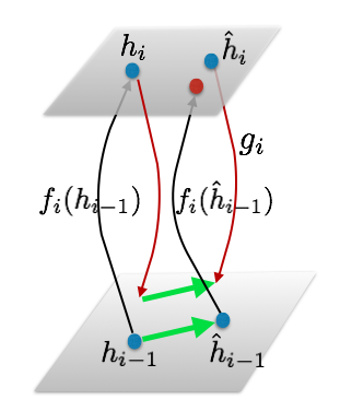
As mentioned above, a required property of target propagation is, that the layer-wise parameter updates, each improving a layer-wise loss, also lead to an improvement of the global loss. The following theorem shows that, for the case that is a perfect inverse of and having a certain structure, the update direction of target propagation does not deviate more then 90 degrees from the gradient direction (estimated by back-propagation), which always leads to a decrease of the global loss.
Theorem 2.1
222See the proof in the Appendix.Assume that , and satisfies 333This is another way to obtain a non-linear deep network structure. where can be any differentiable monotonically increasing element-wise function. Let and be the target propagation update and the back-propagation update in -th layer, respectively. If in Equation (7) is sufficiently small, then the angle between and is bounded by
| (14) |
Here and are the largest and smallest singular values of , where is the Jacobian matrix of and and are close to 0 if is sufficiently small.
2.3 Difference target propagation
From our experience, the imperfection of the inverse function leads to severe optimization problems when assigning targets based on equation (9). This brought us to propose the following linearly corrected formula for target propagation which we refer to as “difference target propagation”
| (15) |
Note, that if is the inverse of , difference target propagation becomes equivalent to vanilla target propagation as defined in equation (9). The resulting complete training procedure for optimization by difference target propagation is given in Algorithm 1.
In the following, we explain why this linear corrected formula stabilizes the optimization process. In order to achieve stable optimization by target propagation, should approach as approaches . Otherwise, the parameters in lower layers continue to be updated even when an optimum of the global loss is reached already by the upper layers, which then could lead the global loss to increase again. Thus, the condition
| (16) |
greatly improves the stability of the optimization. This holds for vanilla target propagation if , because
| (17) |
Although the condition is not guaranteed to hold for vanilla target propagation if , for difference target propagation it holds by construction, since
| (18) |
Furthermore, under weak conditions on and and if the difference between and is small, we can show for difference target propagation that if the input of the -th layer becomes (i.e. the -th layer reaches its target) the output of the -th layer also gets closer to . This means that the requirement on targets specified by equation (6) is met for difference target propagation, as shown in the following theorem
Theorem 2.2
444See the proof in Appendix.Let the target for layer be given by Equation (15), i.e. . If is sufficiently small, and are differentiable, and the corresponding Jacobian matrices and satisfy that the largest eigenvalue of is less than , then we have
| (19) |
The third condition in the above theorem is easily satisfied in practice, because is learned to be the inverse of and makes close to the identity mapping, so that becomes close to the zero matrix which means that the largest eigenvalue of is also close to .
2.4 Training an auto-encoder with difference target propagation
Auto-encoders are interesting for learning representations and serve as building blocks for deep neural networks [10]. In addition, as we have seen, training auto-encoders is part of the target propagation approach presented here, where they model the feedback paths used to propagate the targets.
In the following, we show how a regularized auto-encoder can be trained using difference target propagation instead of back-propagation. Like in the work on denoising auto-encoders [22] and generative stochastic networks [6], we consider the denoising auto-encoder like a stochastic network with noise injected in input and hidden units, trained to minimize a reconstruction loss. This is, the hidden units are given by the encoder as
| (20) |
where is the element-wise sigmoid function, the weight matrix and the bias vector of the input units. The reconstruction is given by the decoder
| (21) |
with being the bias vector of the hidden units. And the reconstruction loss is
| (22) |
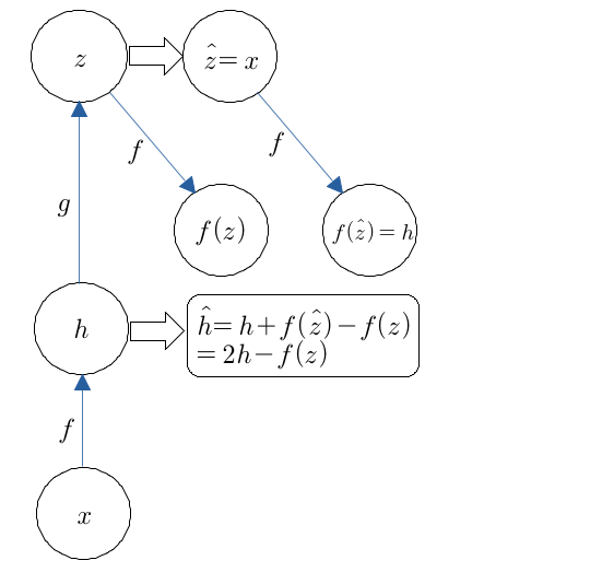
where a regularization term can be added to obtain a contractive mapping. In order to train this network without back-propagation (that is, without using the chain rule), we can use difference target propagation as follows (see Figure 1 (right) for an illustration): at first, the target of is just , so we can train the reconstruction mapping based on the loss in which is considered as a constant. Then, we compute the target of the hidden units following difference target propagation where we make use of the fact that is an approximate inverse of . That is,
| (23) |
where the last equality follows from . As a target loss for the hidden layer, we can use , where is considered as a constant and which can be also augmented by a regularization term to yield a contractive mapping.
3 Experiments
In a set of experiments we investigated target propagation for training deep feedforward deterministic neural networks, networks with discrete transmissions between units, stochastic neural networks, and auto-encoders.
For training supervised neural networks, we chose the target of the top hidden layer (number ) such that it also depends directly on the global loss instead of an inverse mapping. That is, we set , where is the global loss (here the multiclass cross entropy). This may be helpful when the number of units in the output layer is much smaller than the number of units in the top hidden layer, which would make the inverse mapping difficult to learn, but future work should validate that.
For discrete stochastic networks in which some form of noise (here Gaussian) is injected, we used a decaying noise level for learning the inverse mapping, in order to stabilize learning, i.e. the standard deviation of the Gaussian is set to where is the initial value, is the epoch number and is the half-life of this decay. This seems to help to fine-tune the feedback weights at the end of training.
In all experiments, the weights were initialized with orthogonal random matrices and the bias parameters were initially set to zero. All experiments were repeated 10 times with different random initializations. We put the code of these experiments online (https://github.com/donghyunlee/dtp).
3.1 Deterministic feedforward deep networks
As a primary objective, we investigated training of ordinary deep supervised networks with continuous and deterministic units on the MNIST dataset. We used a held-out validation set of 10000 samples for choosing hyper-parameters. We trained networks with 7 hidden layers each consisting of 240 units (using the hyperbolic tangent as activation function) with difference target propagation and back-propagation.
Training was based on RMSprop [21] where hyper-parameters for the best validation error were found using random search [7]. RMSprop is an adaptive learning rate algorithm known to lead to good results for back-propagation. Furthermore, it is suitable for updating the parameters of each layer based on the layer-wise targets obtained by target propagation. Our experiments suggested that when using a hand-selected learning rate per layer rather than the automatically set one (by RMSprop), the selected learning rates were different for each layer, which is why we decided to use an adaptive method like RMSprop.
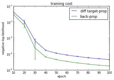
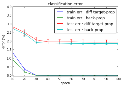
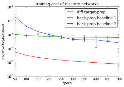
The results are shown in Figure 2. We obtained a test error of 1.94% with target propagation and 1.86% with back propagation. The final negative log-likelihood on the training set was with target propagation and with back propagation. We also trained the same network with rectifier linear units and got a test error of 3.15% whereas 1.62% was obtained with back-propagation. It is well known that this nonlinearity is advantageous for back-propagation, while it seemed to be less appropriate for this implementation of target propagation.
In a second experiment we investigated training on CIFAR-10. The experimental setting was the same as for MNIST (using the hyperbolic tangent as activation function) except that the network architecture was 3072-1000-1000-1000-10. We did not use any preprocessing, except for scaling the input values to lay in [0,1], and we tuned the hyper-parameters of RMSprop using a held-out validation set of 1000 samples. We obtained mean test accuracies of 50.71% and 53.72% for target propagation and back-propagation, respectively. It was reported in [14], that a network with 1 hidden layer of 1000 units achieved 49.78% accuracy with back-propagation, and increasing the number of units to 10000 led to 51.53% accuracy. As the current state-of-the-art performance on the permutation invariant CIFAR-10 recognition task, [12] reported 64.1% but when using PCA without whitening as preprocessing and zero-biased auto-encoders for unsupervised pre-training.
3.2 Networks with discretized transmission between units
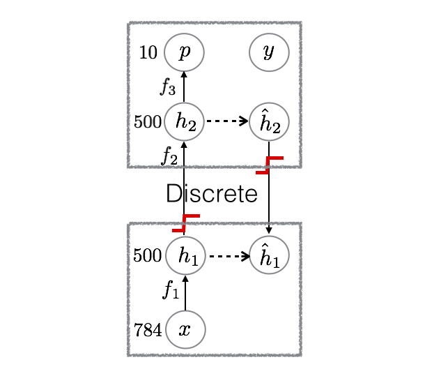
To explore target propagation for an extremely non-linear neural network, we investigated training of discrete networks on the MNIST dataset. The network architecture was 784-500-500-10, where only the 1st hidden layer was discretized. Inspired by biological considerations and the objective of reducing the communication cost between neurons, instead of just using the step activation function, we used ordinary neural net layers but with signals being discretized when transported between the first and second layer. The network structure is depicted in the right plot of Figure 3 and the activations of the hidden layers are given by
| (24) |
where if , and if . The network output is given by
| (25) |
The inverse mapping of the second layer and the associated loss are given by
| (26) |
| (27) |
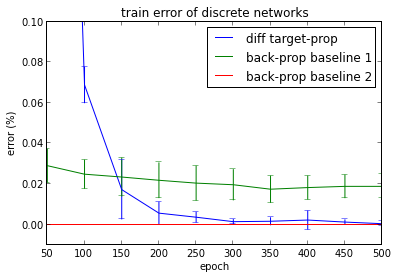
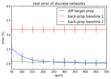
If feed-forward mapping is discrete, back-propagated gradients become 0 and useless when they cross the discretization step. So we compare target propagation to two baselines. As a first baseline, we train the network with back-propagation and the straight-through estimator [5], which is biased but was found to work well, and simply ignores the derivative of the step function (which is 0 or infinite) in the back-propagation phase. As a second baseline, we train only the upper layers by back-propagation, while not changing the weight which are affected by the discretization, i.e., the lower layers do not learn.
The results on the training and test sets are shown in Figure 3. The training error for the first baseline (straight-through estimator) does not converge to zero (which can be explained by the biased gradient) but generalization performance is fairly good. The second baseline (fixed lower layer) surprisingly reached zero training error, but did not perform well on the test set. This can be explained by the fact that it cannot learn any meaningful representation at the first layer. Target propagation however did not suffer from this drawback and can be used to train discrete networks directly (training signals can pass the discrete region successfully). Though the training convergence was slower, the training error did approach zero. In addition, difference target propagation also achieved good results on the test set.
3.3 Stochastic networks
Another interesting model class which vanilla back-propagation cannot deal with are stochastic networks with discrete units. Recently, stochastic networks have attracted attention [3, 20, 5] because they are able to learn a multi-modal conditional distribution , which is important for structured output predictions. Training networks of stochastic binary units is also biologically motivated, since they resemble networks of spiking neurons. Here, we investigate whether one can train networks of stochastic binary units on MNIST for classification using target propagation. Following [17], the network architecture was 784-200-200-10 and the hidden units were stochastic binary units with the probability of turning on given by a sigmoid activation:
| (28) |
that is, is one with probability .
As a baseline, we considered training based on the straight-through biased gradient estimator [5] in which the derivative through the discrete sampling step is ignored (this method showed the best performance in [17].) That is
| (29) |
With difference target propagation the stochastic network can be trained directly, setting the targets to
| (30) |
where is trained by the loss
| (31) |
and layer-local target losses are defined as .
| Method | Test Error(%) |
| Difference Target-Propagation, M=1 | 1.54% |
| Straight-through gradient estimator [5] + backprop, M=1 | |
| as reported in Raiko et al. [17] | 1.71% |
| as reported in Tang and Salakhutdinov [20], M=20 | 3.99% |
| as reported in Raiko et al. [17], M=20 | 1.63% |
For evaluation, we averaged the output probabilities for a given input over 100 samples, and classified the example accordingly, following [17]. Results are given in Table 1. We obtained a test error of 1.71% using the baseline method and 1.54% using target propagation, which is – to our knowledge – the best result for stochastic nets on MNIST reported so far. This suggests that target propagation is highly promising for training networks of binary stochastic units.
3.4 Auto-encoder
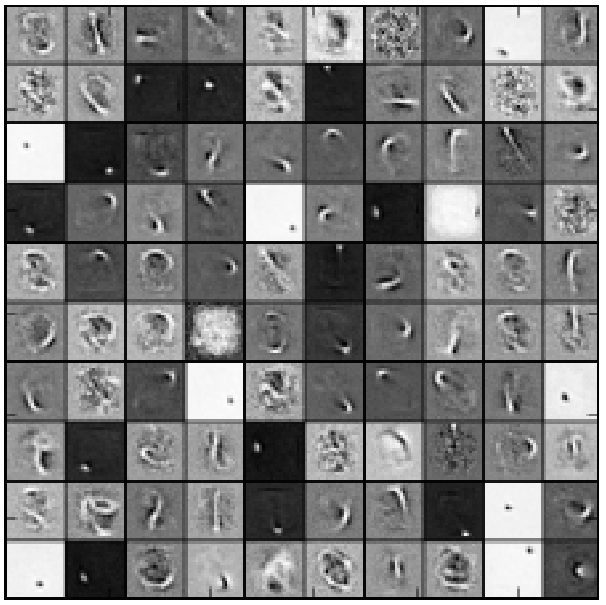
We trained a denoising auto-encoder with 1000 hidden units with difference target propagation as described in Section 2.4 on MNIST. As shown in Figure 4 stroke-like filters can be obtained by target propagation. After supervised fine-tuning (using back-propagation), we got a test error of 1.35. Thus, by training an auto-encoder with target propagation one can learn a good initial representation, which is as good as the one obtained by regularized auto-encoders trained by back-propagation on the reconstruction error.
4 Conclusion
We introduced a novel optimization method for neural networks, called target propagation, which was designed to overcome drawbacks of back-propagation and is biologically more plausible. Target propagation replaces training signals based on partial derivatives by targets which are propagated based on an auto-encoding feedback loop. Difference target propagation is a linear correction for this imperfect inverse mapping which is effective to make target propagation actually work. Our experiments show that target propagation performs comparable to back-propagation on ordinary deep networks and denoising auto-encoders. Moreover, target propagation can be directly used on networks with discretized transmission between units and reaches state of the art performance for stochastic neural networks on MNIST.
Acknowledgments
We would like to thank Junyoung Chung for providing RMSprop code, Caglar Gulcehre and Antoine Biard for general discussion and feedback, Jyri Kivinen for discussion of backprop-free auto-encoder, Mathias Berglund for explanation of his stochastic networks. We thank the developers of Theano [8, 1], a Python library which allowed us to easily develop a fast and optimized code for GPU. We are also grateful for funding from NSERC, the Canada Research Chairs, Compute Canada, and CIFAR.
References
- Bastien et al. [2012] Bastien, F., Lamblin, P., Pascanu, R., Bergstra, J., Goodfellow, I.J., Bergeron, A., Bouchard, N., Bengio, Y.: Theano: new features and speed improvements. Deep Learning and Unsupervised Feature Learning NIPS 2012 Workshop (2012)
- Bengio [2009] Bengio, Y.: Learning deep architectures for AI. Now Publishers (2009)
- Bengio [2013] Bengio, Y.: Estimating or propagating gradients through stochastic neurons. Tech. Rep. arXiv:1305.2982, Universite de Montreal (2013)
- Bengio [2014] Bengio, Y.: How auto-encoders could provide credit assignment in deep networks via target propagation. Tech. rep., arXiv:1407.7906 (2014)
- Bengio et al. [2013] Bengio, Y., Léonard, N., Courville, A.: Estimating or propagating gradients through stochastic neurons for conditional computation. arXiv:1308.3432 (2013)
- Bengio et al. [2014] Bengio, Y., Thibodeau-Laufer, E., Yosinski, J.: Deep generative stochastic networks trainable by backprop. In: ICML’2014 (2014)
- Bergstra and Bengio [2012] Bergstra, J., Bengio, Y.: Random search for hyper-parameter optimization. J. Machine Learning Res. 13, 281–305 (2012)
- Bergstra et al. [2010] Bergstra, J., Breuleux, O., Bastien, F., Lamblin, P., Pascanu, R., Desjardins, G., Turian, J., Warde-Farley, D., Bengio, Y.: Theano: a CPU and GPU math expression compiler. In: Proceedings of the Python for Scientific Computing Conference (SciPy) (Jun 2010), oral Presentation
- Carreira-Perpinan and Wang [2014] Carreira-Perpinan, M., Wang, W.: Distributed optimization of deeply nested systems. In: AISTATS’2014, JMLR W&CP. vol. 33, pp. 10–19 (2014)
- Erhan et al. [2010] Erhan, D., Courville, A., Bengio, Y., Vincent, P.: Why does unsupervised pre-training help deep learning? In: JMLR W&CP: Proc. AISTATS’2010. vol. 9, pp. 201–208 (2010)
- Hinton et al. [2012] Hinton, G., Deng, L., Dahl, G.E., Mohamed, A., Jaitly, N., Senior, A., Vanhoucke, V., Nguyen, P., Sainath, T., Kingsbury, B.: Deep neural networks for acoustic modeling in speech recognition. IEEE Signal Processing Magazine 29(6), 82–97 (Nov 2012)
- Konda et al. [2015] Konda, K., Memisevic, R., Krueger, D.: Zero-bias autoencoders and the benefits of co-adapting features. Under review on International Conference on Learning Representations (2015)
- Krizhevsky et al. [2012] Krizhevsky, A., Sutskever, I., Hinton, G.: ImageNet classification with deep convolutional neural networks. In: NIPS’2012 (2012)
- Krizhevsky and Hinton [2009] Krizhevsky, A., Hinton, G.: Learning multiple layers of features from tiny images. Master’s thesis, University of Toronto (2009)
- LeCun [1986] LeCun, Y.: Learning processes in an asymmetric threshold network. In: Fogelman-Soulié, F., Bienenstock, E., Weisbuch, G. (eds.) Disordered Systems and Biological Organization, pp. 233–240. Springer-Verlag, Les Houches, France (1986)
- LeCun [1987] LeCun, Y.: Modèles connexionistes de l’apprentissage. Ph.D. thesis, Université de Paris VI (1987)
- Raiko et al. [2014] Raiko, T., Berglund, M., Alain, G., Dinh, L.: Techniques for learning binary stochastic feedforward neural networks. NIPS Deep Learning Workshop 2014 (2014)
- Sutskever et al. [2014] Sutskever, I., Vinyals, O., Le, Q.V.: Sequence to sequence learning with neural networks. Tech. rep., arXiv:1409.3215 (2014)
- Szegedy et al. [2014] Szegedy, C., Liu, W., Jia, Y., Sermanet, P., Reed, S., Anguelov, D., Erhan, D., Vanhoucke, V., Rabinovich, A.: Going deeper with convolutions. Tech. rep., arXiv:1409.4842 (2014)
- Tang and Salakhutdinov [2013] Tang, Y., Salakhutdinov, R.: A new learning algorithm for stochastic feedforward neural nets. ICML’2013 Workshop on Challenges in Representation Learning (2013)
- Tieleman and Hinton [2012] Tieleman, T., Hinton, G.: Lecture 6.5-rmsprop: Divide the gradient by a running average of its recent magnitude. COURSERA: Neural Networks for Machine Learning 4 (2012)
- Vincent et al. [2010] Vincent, P., Larochelle, H., Lajoie, I., Bengio, Y., Manzagol, P.A.: Stacked denoising autoencoders: Learning useful representations in a deep network with a local denoising criterion. J. Machine Learning Res. 11 (2010)
Appendix
Appendix 0.A Proof of Theorem 1
Proof
Given a training example the back-propagation update is given by
where . Here is a diagonal matrix with each diagonal element being element-wise derivatives and is the Jacobian of . In target propagation the target for is given by . If all ’s are allocated in smooth areas and is sufficiently small, we can apply a Taylor expansion to get
where is the remainder satisfying . Now, for we have
We write as l , as v and as for short. Then the inner production of vector forms of and is
For and we have
and similarly
where and are matrix Euclidean norms, i.e. the largest singular value of , , and the largest singular value of , ( is the smallest singular value of , because is invertable, so all the smallest singular values of Jacobians are larger than ). Finally, if is sufficiently small, the angle between and satisfies:
where the last expression is positive if is sufficiently small and is trivial.
Appendix 0.B Proof of Theorem 2
Proof
Let . Applying Taylor’s theorem twice, we get
where the vector represents the remainder satisfying . Then for we have
| (A-1) | |||||
where is the scalar value resulting from all terms depending on and is the
largest eigenvalue of
.
If is sufficiently small to guarantee
,
then the left of Equation (A-1) is less than which is just
.