Striving for Simplicity:
The All Convolutional Net
Abstract
Most modern convolutional neural networks (CNNs) used for object recognition are built using the same principles: Alternating convolution and max-pooling layers followed by a small number of fully connected layers. We re-evaluate the state of the art for object recognition from small images with convolutional networks, questioning the necessity of different components in the pipeline. We find that max-pooling can simply be replaced by a convolutional layer with increased stride without loss in accuracy on several image recognition benchmarks. Following this finding – and building on other recent work for finding simple network structures – we propose a new architecture that consists solely of convolutional layers and yields competitive or state of the art performance on several object recognition datasets (CIFAR-10, CIFAR-100, ImageNet). To analyze the network we introduce a new variant of the “deconvolution approach” for visualizing features learned by CNNs, which can be applied to a broader range of network structures than existing approaches.
1 Introduction and Related Work
The vast majority of modern convolutional neural networks (CNNs) used for object recognition are built using the same principles: They use alternating convolution and max-pooling layers followed by a small number of fully connected layers (e.g. Jarrett et al. (2009); Krizhevsky et al. (2012); Ciresan et al. ). Within each of these layers piecewise-linear activation functions are used. The networks are typically parameterized to be large and regularized during training using dropout. A considerable amount of research has over the last years focused on improving the performance of this basic pipeline. Among these two major directions can be identified. First, a plethora of extensions were recently proposed to enhance networks which follow this basic scheme. Among these the most notable directions are work on using more complex activation functions (Goodfellow et al., 2013; Lin et al., 2014; Srivastava et al., 2013) techniques for improving class inference (Stollenga et al., 2014; Srivastava & Salakhutdinov, 2013) as well as procedures for improved regularization (Zeiler & Fergus, 2013; Springenberg & Riedmiller, 2013; Wan et al., 2013) and layer-wise pre-training using label information (Lee et al., 2014). Second, the success of CNNs for large scale object recognition in the ImageNet challenge (Krizhevsky et al., 2012) has stimulated research towards experimenting with the different architectural choices in CNNs. Most notably the top entries in the 2014 ImageNet challenge deviated from the standard design principles by either introducing multiple convolutions in between pooling layers (Simonyan & Zisserman, 2014) or by building heterogeneous modules performing convolutions and pooling at multiple scales in each layer (Szegedy et al., 2014).
Since all of these extensions and different architectures come with their own parameters and training procedures the question arises which components of CNNs are actually necessary for achieving state of the art performance on current object recognition datasets. We take a first step towards answering this question by studying the most simple architecture we could conceive: a homogeneous network solely consisting of convolutional layers, with occasional dimensionality reduction by using a stride of 2. Surprisingly, we find that this basic architecture – trained using vanilla stochastic gradient descent with momentum – reaches state of the art performance without the need for complicated activation functions, any response normalization or max-pooling. We empirically study the effect of transitioning from a more standard architecture to our simplified CNN by performing an ablation study on CIFAR-10 and compare our model to the state of the art on CIFAR-10, CIFAR-100 and the ILSVRC-2012 ImageNet dataset. Our results both confirm the effectiveness of using small convolutional layers as recently proposed by Simonyan & Zisserman (2014) and give rise to interesting new questions about the necessity of pooling in CNNs. Since dimensionality reduction is performed via strided convolution rather than max-pooling in our architecture it also naturally lends itself to studying questions about the invertibility of neural networks (Estrach et al., 2014). For a first step in that direction we study properties of our network using a deconvolutional approach similar to Zeiler & Fergus (2014).
2 Model description - the all convolutional network
The models we use in our experiments differ from standard CNNs in several key aspects. First – and most interestingly – we replace the pooling layers, which are present in practically all modern CNNs used for object recognition, with standard convolutional layers with stride two. To understand why this procedure can work it helps to recall the standard formulation for defining convolution and pooling operations in CNNs. Let denote a feature map produced by some layer of a CNN. It can be described as a 3-dimensional array of size where and are the width and height and is the number of channels (in case is the output of a convolutional layer, is the number of filters in this layer). Then p-norm subsampling (or pooling) with pooling size (or half-length ) and stride applied to the feature map is a 3-dimensional array with the following entries:
| (1) |
where is the function mapping from positions in to positions in respecting the stride, is the order of the p-norm (for , it becomes the commonly used max pooling). If , pooling regions do not overlap; however, current CNN architectures typically include overlapping pooling with and . Let us now compare the pooling operation defined by Eq. 1 to the standard definition of a convolutional layer applied to feature map given as:
| (2) |
where are the convolutional weights (or the kernel weights, or filters), is the activation function, typically a rectified linear activation ReLU , and is the number of output feature (or channel) of the convolutional layer. When formalized like this it becomes clear that both operations depend on the same elements of the previous layer feature map. The pooling layer can be seen as performing a feature-wise convolution 111That is, a convolution where if equals and zero otherwise. in which the activation function is replaced by the p-norm. One can therefore ask the question whether and why such special layers need to be introduced into the network. While a complete answer of this question is not easy to give (see the experiments and discussion for further details and remarks) we assume that in general there exist three possible explanations why pooling can help in CNNs: 1) the p-norm makes the representation in a CNN more invariant; 2) the spatial dimensionality reduction performed by pooling makes covering larger parts of the input in higher layers possible; 3) the feature-wise nature of the pooling operation (as opposed to a convolutional layer where features get mixed) could make optimization easier. Assuming that only the second part – the dimensionality reduction performed by pooling – is crucial for achieving good performance with CNNs (a hypothesis that we later test in our experiments) one can now easily see that pooling can be removed from a network without abandoning the spatial dimensionality reduction by two means:
-
1.
We can remove each pooling layer and increase the stride of the convolutional layer that preceded it accordingly.
-
2.
We can replace the pooling layer by a normal convolution with stride larger than one (i.e. for a pooling layer with and we replace it with a convolution layer with corresponding stride and kernel size and number of output channels equal to the number of input channels)
The first option has the downside that we significantly reduce the overlap of the convolutional layer that preceded the pooling layer. It is equivalent to a pooling operation in which only the top-left feature response is considered and can result in less accurate recognition. The second option does not suffer from this problem, since all existing convolutional layers stay unchanged, but results in an increase of overall network parameters. It is worth noting that replacing pooling by convolution adds inter-feature dependencies unless the weight matrix is constrained. We emphasize that that this replacement can also be seen as learning the pooling operation rather than fixing it; which has previously been considered using different parameterizations in the literature 222Although in order to implement “proper pooling” in the same sense as commonly considered in the literature a special nonlinearity (e.g. a squaring operation) needs to be considered. A simple convolution layer with rectified linear activation cannot by itself implement a p-norm computation. (LeCun et al., 1998; Gülçehre et al., 2014; Jia et al., 2012). We will evaluate both options in our experiments, ensuring a fair comparison w.r.t. the number of network parameters. Although we are not aware of existing studies containing such controlled experiments on replacing pooling with convolution layers it should be noted that the idea of removing pooling is not entirely unprecedented: First, the nomenclature in early work on CNNs LeCun et al. (1998) (referring to pooling layers as subsampling layers already) suggests the usage of different operations for subsampling. Second, albeit only considering small networks, experiments on using only convolution layers (with occasional subsampling) in an architecture similar to traditional CNNs already appeared in work on the “neural abstraction pyramid”Behnke (2003).
The second difference of the network model we consider to standard CNNs is that – similar to models recently used for achieving state-of-the-art performance in the ILSVRC-2012 competition (Simonyan & Zisserman, 2014; Szegedy et al., 2014) – we make use of small convolutional layers with which can greatly reduce the number of parameters in a network and thus serve as a form of regularization. Additionally, to unify the architecture further, we make use of the fact that if the image area covered by units in the topmost convolutional layer covers a portion of the image large enough to recognize its content (i.e. the object we want to recognize) then fully connected layers can also be replaced by simple 1-by-1 convolutions. This leads to predictions of object classes at different positions which can then simply be averaged over the whole image. This scheme was first described by Lin et al. (2014) and further regularizes the network as the one by one convolution has much less parameters than a fully connected layer. Overall our architecture is thus reduced to consist only of convolutional layers with rectified linear non-linearities and an averaging + softmax layer to produce predictions over the whole image.
| Model | ||
| A | B | C |
| Input RGB image | ||
| conv. ReLU | conv. ReLU | conv. ReLU |
| conv. ReLU | conv. ReLU | |
| max-pooling stride | ||
| conv. ReLU | conv. ReLU | conv. ReLU |
| conv. ReLU | conv. ReLU | |
| max-pooling stride | ||
| conv. ReLU | ||
| conv. ReLU | ||
| conv. ReLU | ||
| global averaging over spatial dimensions | ||
| 10 or 100-way softmax | ||
3 Experiments
In order to quantify the effect of simplifying the model architecture we perform experiments on three datasets: CIFAR-10, CIFAR-100 (Krizhevsky & Hinton, 2009) and ILSVRC-2012 ImageNet (Deng et al., 2009) . Specifically, we use CIFAR-10 to perform an in-depth study of different models, since a large model on this dataset can be trained with moderate computing costs of hours on a modern GPU. We then test the best model found on CIFAR-10 and CIFAR-100 with and without augmentations and perform a first preliminary experiment on the ILSVRC-2012 ImageNet dataset. We performed all experiments using the Caffe (Jia et al., 2014) framework.
3.1 Experimental Setup
In experiments on CIFAR-10 and CIFAR-100 we use three different base network models which are intended to reflect current best practices for setting up CNNs for object recognition. Architectures of these networks are described in Table 1. Starting from model A (the simplest model) the depth and number of parameters in the network gradually increases to model C. Several things are to be noted here. First, as described in the table, all base networks we consider use a 1-by-1 convolution at the top to produce 10 outputs of which we then compute an average over all positions and a softmax to produce class-probabilities (see Section 2 for the rationale behind this approach). We performed additional experiments with fully connected layers instead of 1-by-1 convolutions but found these models to consistently perform worse than their fully convolutional counterparts. This is in line with similar findings from prior work (Lin et al., 2014). We hence do not report these numbers here to avoid cluttering the experiments. Second, it can be observed that model B from the table is a variant of the Network in Network architecture proposed by Lin et al. (2014) in which only one 1-by-1 convolution is performed after each “normal” convolution layer. Third, model C replaces all convolutions by simple convolutions. This serves two purposes: 1) it unifies the architecture to consist only of layers operating on spatial neighborhoods of the previous layer feature map (with occasional subsampling); 2) if max-pooling is replaced by a convolutional layer, then is the minimum filter size to allow overlapping convolution with stride 2. We also highlight that model C resembles the very deep models used by Simonyan & Zisserman (2014) in this years ImageNet competition.
| Model | ||
| Strided-CNN-C | ConvPool-CNN-C | All-CNN-C |
| Input RGB image | ||
| conv. ReLU | conv. ReLU | conv. ReLU |
| conv. ReLU | conv. ReLU | conv. ReLU |
| with stride | conv. ReLU | |
| max-pooling stride | conv. ReLU | |
| with stride | ||
| conv. ReLU | conv. ReLU | conv. ReLU |
| conv. ReLU | conv. ReLU | conv. ReLU |
| with stride | conv. ReLU | |
| max-pooling stride | conv. ReLU | |
| with stride | ||
For each of the base models we then experiment with three additional variants. The additional (derived) models for base model C are described in in Table 2. The derived models for base models A and B are built analogously but not shown in the table to avoid cluttering the paper. In general the additional models for each base model consist of:
-
•
A model in which max-pooling is removed and the stride of the convolution layers preceding the max-pool layers is increased by 1 (to ensure that the next layer covers the same spatial region of the input image as before). This is column “Strided-CNN-C” in the table.
-
•
A model in which max-pooling is replaced by a convolution layer. This is column “All-CNN-C” in the table.
-
•
A model in which a dense convolution is placed before each max-pooling layer (the additional convolutions have the same kernel size as the respective pooling layer). This is model “ConvPool-CNN-C” in the table. Experiments with this model are necessary to ensure that the effect we measure is not solely due to increasing model size when going from a “normal” CNN to its “All-CNN” counterpart.
Finally, to test whether a network solely using convolutions also performs well on a larger scale recognition problem we trained an up-scaled version of ALL-CNN-B on the ILSVRC 2012 part of the ImageNet database. Although we expect that a larger network using only convolutions and having stride in the first layer (and thus similar in style to Simonyan & Zisserman (2014)) would perform even better on this dataset, training it would take several weeks and could thus not be completed in time for this manuscript.
3.2 Classification results
3.2.1 CIFAR-10
| CIFAR-10 classification error | ||
|---|---|---|
| Model | Error () | # parameters |
| without data augmentation | ||
| Model A | M | |
| Strided-CNN-A | M | |
| ConvPool-CNN-A | M | |
| ALL-CNN-A | M | |
| Model B | M | |
| Strided-CNN-B | M | |
| ConvPool-CNN-B | M | |
| ALL-CNN-B | M | |
| Model C | M | |
| Strided-CNN-C | M | |
| ConvPool-CNN-C | M | |
| ALL-CNN-C | M | |
In our first experiment we compared all models from Section 3.1 on the CIFAR-10 dataset without using any augmentations. All networks were trained using stochastic gradient descent with fixed momentum of . The learning rate was adapted using a schedule in which is multiplied by a fixed multiplier of after and epochs respectively. To keep the amount of computation necessary to perform our comparison bearable 333Training one network on CIFAR-10 can take up to 10 hours on a modern GPU. we only treat as a changeable hyperparameter for each method. The learning rate schedule and the total amount of training epochs were determined in a preliminary experiment using base model A and then fixed for all other experiments. We used and trained all networks for a total of 350 epochs. It should be noted that this strategy is not guaranteed to result in the best performance for all methods and thus care must be taken when interpreting the the following results from our experiments. The learning rate was individually adapted for each model by searching over the fixed set . In the following we only report the results for the best for each method. Dropout (Hinton et al., 2012) was used to regularize all networks. We applied dropout to the input image as well as after each pooling layer (or after the layer replacing the pooling layer respectively). The dropout probabilities were for dropping out inputs and otherwise. We also experimented with additional dropout (i.e. dropout on all layers or only on the convolution layer) which however did not result in increased accuracy444In the case were dropout of 0.5 is applied to all layers accuracy even dropped, suggesting that the gradients become too noisy in this case . Additionally all models were regularized with weight decay . In experiments with data augmentation we perform only the augmentations also used in previous work (Goodfellow et al., 2013; Lin et al., 2014) in order to keep our results comparable. These include adding horizontally flipped examples of all images as well as randomly translated versions (with a maximum translation of 5 pixels in each dimension). In all experiments images were whitened and contrast normalized following Goodfellow et al. (2013).
The results for all models that we considered are given in Table 3. Several trends can be observed from the table. First, confirming previous results from the literature (Srivastava et al., 2014) the simplest model (model A) already performs remarkably well, achieving error. Second, simply removing the max-pooling layer and just increasing the stride of the previous layer results in diminished performance in all settings. While this is to be expected we can already see that the drop in performance is not as dramatic as one might expect from such a drastic change to the network architecture. Third, surprisingly, when pooling is replaced by an additional convolution layer with stride performance stabilizes and even improves on the base model. To check that this is not only due to an increase in the number of trainable parameters we compare the results to the “ConvPool” versions of the respective base model. In all cases the performance of the model without any pooling and the model with pooling on top of the additional convolution perform about on par. Surprisingly, this suggests that while pooling can help to regularize CNNs, and generally does not hurt performance, it is not strictly necessary to achieve state-of-the-art results (at least for current small scale object recognition datasets). In addition, our results confirm that small convolutions stacked after each other seem to be enough to achieve the best performance.
Perhaps even more interesting is the comparison between the simple all convolutional network derived from base model C and the state of the art on CIFAR-10 shown in Table 4 , both with and without data augmentation. In both cases the simple network performs better than the best previously reported result. This suggests that in order to perform well on current benchmarks “almost all you need” is a stack of convolutional layers with occasional stride of to perform subsampling.
| CIFAR-10 classification error | ||
|---|---|---|
| Method | Error () | # params |
| without data augmentation | ||
| Maxout [1] | M | |
| Network in Network [2] | M | |
| Deeply Supervised [3] | M | |
| ALL-CNN (Ours) | M | |
| with data augmentation | ||
| Maxout [1] | M | |
| DropConnect [2] | - | |
| dasNet [4] | M | |
| Network in Network [2] | M | |
| Deeply Supervised [3] | M | |
| ALL-CNN (Ours) | M | |
| CIFAR-100 classification error | |
|---|---|
| Method | Error () |
| CNN + tree prior [5] | |
| Network in Network [2] | |
| Deeply Supervised [3] | |
| Maxout (larger) [4] | |
| dasNet [4] | |
| ALL-CNN (Ours) | |
| Fractional Pooling (1 test) [6] | |
| Fractional Pooling (12 tests) [6] | |
| CIFAR-10 classification error | |
|---|---|
| Method | Error () |
| with large data augmentation | |
| Spatially Sparse CNN [6] | |
| Large ALL-CNN (Ours) | |
| Fractional Pooling (1 test) [6] | |
| Fractional Pooling (100 tests) [6] | |
3.2.2 CIFAR-100
We performed an additional experiment on the CIFAR-100 dataset to confirm the efficacy of the best model (the All-CNN-C) found for CIFAR-10. As is common practice we used the same model as on CIFAR-10 and also kept all hyperparameters (the learning rate as well as its schedule) fixed. Again note that this does not necessarily give the best performance. The results of this experiment are given in Table 4 (right). As can be seen, the simple model using only convolutions again performs comparable to the state of the art for this dataset even though most of the other methods either use more complicated training schemes or network architectures. It is only outperformed by the fractional max-pooling approach (Graham, 2015) which uses a much larger network (on the order of parameters).
3.2.3 CIFAR-10 with additional data augmentation
After performing our experiments we became aware of recent results by Graham (2015) who report a new state of the art on CIFAR-10/100 with data augmentation. These results were achieved using very deep CNNs with convolution layers in combination with aggressive data augmentation in which the images are placed into large pixel images and can hence be heavily scaled, rotated and color augmented. We thus implemented the Large-All-CNN, which is the all convolutional version of this network (see Table 5 in the appendix for details) and report the results of this additional experiment in Table 4 (bottom right). As can be seen, Large-All-CNN achieves performance comparable to the network with max-pooling. It is only outperformed by the fractional max-pooling approach when performing multiple passes through the network. Note that these networks have vastly more parameters ( M) than the networks from our previous experiments. We are currently re-training the Large-All-CNN network on CIFAR-100, and will include the results in Table 4 once training is finished.
3.3 Classification of Imagenet
We performed additional experiments using the ILVRC-2012 subset of the ImageNet dataset. Since training a state of the art model on this dataset can take several weeks of computation on a modern GPU, we did not aim for best performance, but rather performed a simple ’proof of concept’ experiment. To test if the architectures performing best on CIFAR-10 also apply to larger datasets, we trained an upscaled version of the All-CNN-B network (which is also similar to the architecture proposed by Lin et al. (2014)). It has 12 convolutional layers (conv1-conv12) and was trained for iterations with batches of samples each, starting with a learning rate of and dividing it by after every iterations. A weight decay of was used in all layers. The exact architecture used is given in Table 6 in the Appendix.
This network achieves a Top-1 validation error of on ILSVRC-2012, when only evaluating on the center patch, – which is comparable to the Top-1 error reported by Krizhevsky et al. (2012) – while having less than million parameters (6 times less than the network of Krizhevsky et al. (2012)) and taking roughly days to train on a Titan GPU. This supports our intuition that max-pooling may not be necessary for training large-scale convolutional networks. However, a more thorough analysis is needed to precisely evaluate the effect of max-pooling on ImageNet-scale networks. Such a complete quantitative analysis using multiple networks on ImageNet is extremely computation-time intensive and thus out of the scope of this paper. In order to still gain some insight into the effects of getting rid of max-pooling layers, we will try to analyze the representation learned by the all convolutional network in the next section.
3.4 Deconvolution
In order to analyze the network that we trained on ImageNet – and get a first impression of how well the model without pooling lends itself to approximate inversion – we use a ’deconvolution’ approach. We start from the idea of using a deconvolutional network for visualizing the parts of an image that are most discriminative for a given unit in a network, an approach recently proposed by Zeiler & Fergus (2014). Following this initial attempt – and observing that it does not always work well without max-pooling layers – we propose a new and efficient way of visualizing the concepts learned by higher network layers.
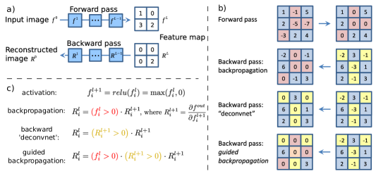
The deconvolutional network (’deconvnet’) approach to visualizing concepts learned by neurons in higher layers of a CNN can be summarized as follows. Given a high-level feature map, the ’deconvnet’ inverts the data flow of a CNN, going from neuron activations in the given layer down to an image. Typically, a single neuron is left non-zero in the high level feature map. Then the resulting reconstructed image shows the part of the input image that is most strongly activating this neuron (and hence the part that is most discriminative to it). A schematic illustration of this procedure is shown in Figure 1 a). In order to perform the reconstruction through max-pooling layers, which are in general not invertible, the method of Zeiler and Fergus requires first to perform a forward pass of the network to compute ’switches’ – positions of maxima within each pooling region. These switches are then used in the ’deconvnet’ to obtain a discriminative reconstruction. By using the switches from a forward pass the ’deconvnet’ (and thereby its reconstruction) is hence conditioned on an image and does not directly visualize learned features. Our architecture does not include max-pooling, meaning that in theory we can ’deconvolve’ without switches, i.e. not conditioning on an input image.
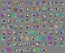
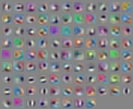
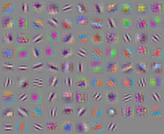
This way we get insight into what lower layers of the network learn. Visualizations of features from the first three layers are shown in Figure 2 . Interestingly, the very first layer of the network does not learn the usual Gabor filters, but higher layers do.
| conv1 | conv2 | conv3 |
|
|
|
For higher layers of our network the method of Zeiler and Fergus fails to produce sharp, recognizable, image structure. This is in agreement with the fact that lower layers learn general features with limited amount of invariance, which allows to reconstruct a single pattern that activates them. However, higher layers learn more invariant representations, and there is no single image maximally activating those neurons. Hence to get reasonable reconstructions it is necessary to condition on an input image.
An alternative way of visualizing the part of an image that most activates a given neuron is to use a simple backward pass of the activation of a single neuron after a forward pass through the network; thus computing the gradient of the activation w.r.t. the image. The backward pass is, by design, partially conditioned on an image through both the activation functions of the network and the max-pooling switches (if present). The connections between the deconvolution and the backpropagation approach were recently discussed in Simonyan et al. (2014). In short the both methods differ mainly in the way they handle backpropagation through the rectified linear (ReLU) nonlinearity.
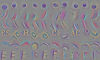
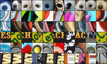
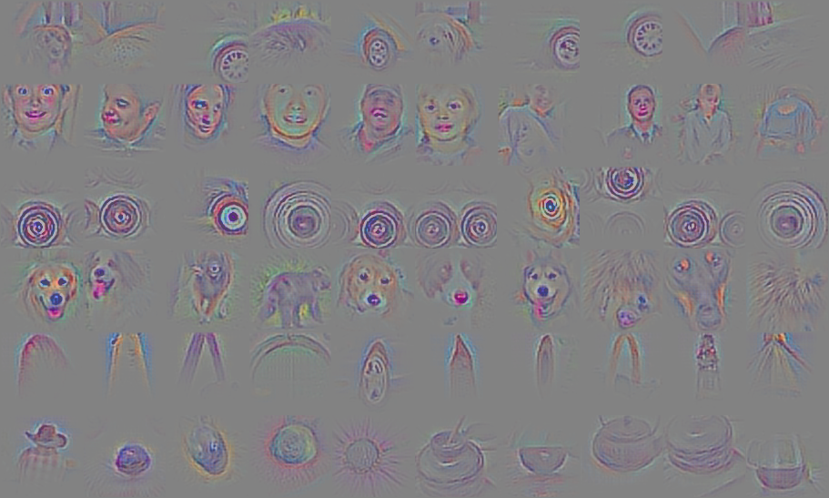
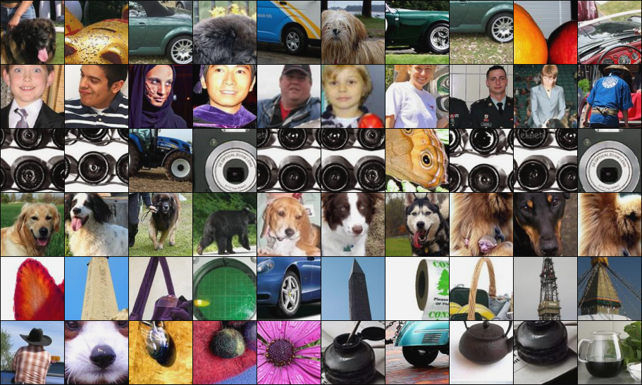
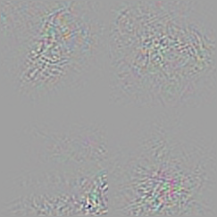
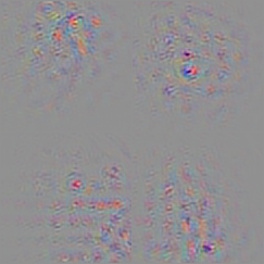
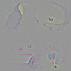
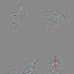
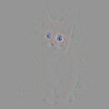
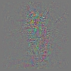
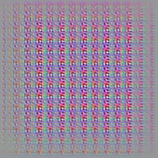
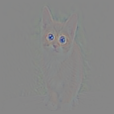
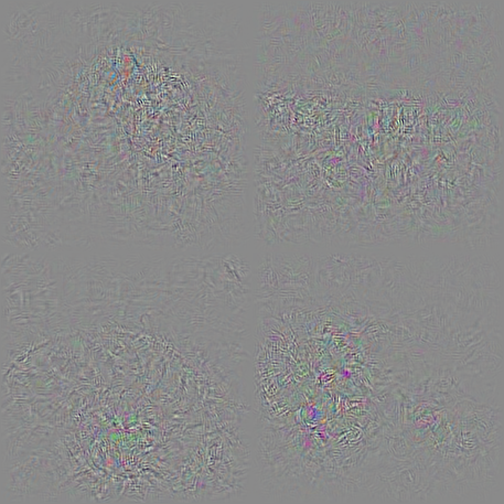
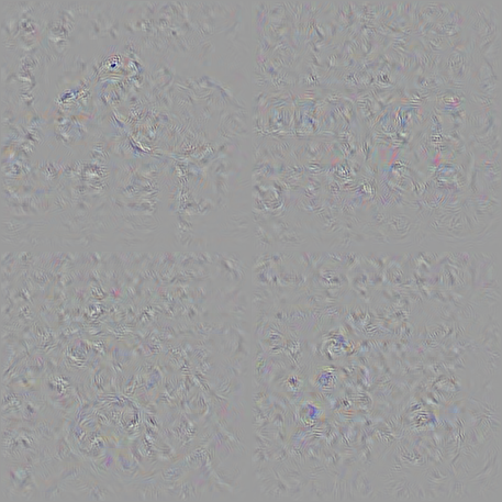
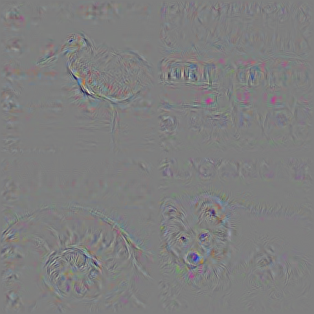
In order to obtain a reconstruction conditioned on an input image from our network without pooling layers we propose a modification of the ’deconvnet’, which makes reconstructions significantly more accurate, especially when reconstructing from higher layers of the network. The ’deconvolution’ is equivalent to a backward pass through the network, except that when propagating through a nonlinearity, its gradient is solely computed based on the top gradient signal, ignoring the bottom input. In case of the ReLU nonlinearity this amounts to setting to zero certain entries based on the top gradient. The two different approaches are depicted in Figure 1 b), rows 2 and 3. We propose to combine these two methods: rather than masking out values corresponding to negative entries of the top gradient (’deconvnet’) or bottom data (backpropagation), we mask out the values for which at least one of these values is negative, see row 4 of Figure 1 b). We call this method guided backpropagation, because it adds an additional guidance signal from the higher layers to usual backpropagation. This prevents backward flow of negative gradients, corresponding to the neurons which decrease the activation of the higher layer unit we aim to visualize. Interestingly, unlike the ’deconvnet’, guided backpropagation works remarkably well without switches, and hence allows us to visualize intermediate layers (Figure 3) as well as the last layers of our network (Figures 4 and 5 in the Appendix). In a sense, the bottom-up signal in form of the pattern of bottom ReLU activations substitutes the switches.
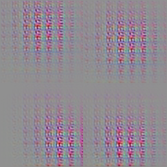
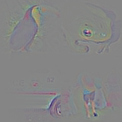
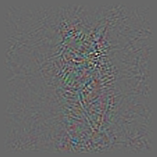
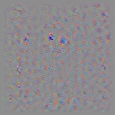
To compare guided backpropagation and the ’deconvnet’ approach, we replace the stride in our network by max-pooling after training, which allows us to obtain the values of switches. We then visualize high level activations using three methods: backpropagation, ’deconvnet’ and guided backpropagation. A striking difference in image quality is visible in the feature visualizations of the highest layers of the network, see Figures 4 and 5 in the Appendix. Guided backpropagation works equally well with and without switches, while the ’deconvnet’ approach fails completely in the absence of switches. One potential reason why the ’deconvnet’ underperforms in this experiment is that max-pooling was only ’artificially’ introduced after training. As a control Figure 6 shows visualizations of units in the fully connected layer of a network initially trained with max-pooling. Again guided backpropagation produces cleaner visualizations than the ’deconvnet’ approach.
4 Discussion
To conclude, we highlight a few key observations that we made in our experiments:
-
•
With modern methods of training convolutional neural networks very simple architectures may perform very well: a network using nothing but convolutions and subsampling matches or even slightly outperforms the state of the art on CIFAR-10 and CIFAR-100. A similar architecture shows competitive results on ImageNet.
-
•
In particular, as opposed to previous observations, including explicit (max-)pooling operations in a network does not always improve performance of CNNs. This seems to be especially the case if the network is large enough for the dataset it is being trained on and can learn all necessary invariances just with convolutional layers.
-
•
We propose a new method of visualizing the representations learned by higher layers of a convolutional network. While being very simple, it produces sharper visualizations of descriptive image regions than the previously known methods, and can be used even in the absence of ’switches’ – positions of maxima in max-pooling regions.
We want to emphasize that this paper is not meant to discourage the use of pooling or more sophisticated activation functions altogether. It should rather be understood as an attempt to both search for the minimum necessary ingredients for recognition with CNNs and establish a strong baseline on often used datasets. We also want to stress that the results of all models evaluated in this paper could potentially be improved by increasing the overall model size or a more thorough hyperparameter search. In a sense this fact makes it even more surprising that the simple model outperforms many existing approaches.
| deconv | guided backpropagation | corresponding image crops |
|---|---|---|
 |
 |
| deconv | guided backpropagation | corresponding image crops |
|---|---|---|
 |
 |
Acknowledgments
We acknowledge funding by the ERC Starting Grant VideoLearn (279401); the work was also partly supported by the BrainLinks-BrainTools Cluster of Excellence funded by the German Research Foundation (DFG, grant number EXC 1086).
References
- Behnke (2003) Behnke, Sven. Hierarchical neural networks for image interpretation. PhD thesis, 2003.
- (2) Ciresan, Dan C., Meier, Ueli, Masci, Jonathan, Gambardella, Luca M., and Schmidhuber, Jürgen. High-performance neural networks for visual object classification. In arxiv:cs/arXiv:1102.0183. URL http://arxiv.org/abs/1102.0183.
- Deng et al. (2009) Deng, Jia, Dong, Wei, Socher, Richard, jia Li, Li, Li, Kai, and Fei-fei, Li. Imagenet: A large-scale hierarchical image database. In CVPR, 2009.
- Estrach et al. (2014) Estrach, Joan B., Szlam, Arthur, and Lecun, Yann. Signal recovery from pooling representations. In ICML, 2014.
- Goodfellow et al. (2013) Goodfellow, Ian J., Warde-Farley, David, Mirza, Mehdi, Courville, Aaron, and Bengio, Yoshua. Maxout networks. In ICML, 2013.
- Graham (2015) Graham, Benjamin. Fractional max-pooling. In arxiv:cs/arXiv:1412.6071, 2015.
- Gülçehre et al. (2014) Gülçehre, Çaglar, Cho, KyungHyun, Pascanu, Razvan, and Bengio, Yoshua. Learned-norm pooling for deep feedforward and recurrent neural networks. In ECML, 2014.
- Hinton et al. (2012) Hinton, Geoffrey E., Srivastava, Nitish, Krizhevsky, Alex, Sutskever, Ilya, and Salakhutdinov, Ruslan R. Improving neural networks by preventing co-adaptation of feature detectors. 2012. pre-print, arxiv:cs/1207.0580v3.
- Jarrett et al. (2009) Jarrett, Kevin, Kavukcuoglu, Koray, Ranzato, Marc’Aurelio, and LeCun, Yann. What is the best multi-stage architecture for object recognition? In ICCV, 2009.
- Jia et al. (2012) Jia, Yangqing, Huang, Chang, and Darrell, Trevor. Beyond spatial pyramids: Receptive field learning for pooled image features. In CVPR, 2012.
- Jia et al. (2014) Jia, Yangqing, Shelhamer, Evan, Donahue, Jeff, Karayev, Sergey, Long, Jonathan, Girshick, Ross, Guadarrama, Sergio, and Darrell, Trevor. Caffe: Convolutional architecture for fast feature embedding. arXiv preprint arXiv:1408.5093, 2014.
- Krizhevsky & Hinton (2009) Krizhevsky, A. and Hinton, G. Learning multiple layers of features from tiny images. 2009.
- Krizhevsky et al. (2012) Krizhevsky, Alex, Sutskever, Ilya, and Hinton, Geoffrey E. Imagenet classification with deep convolutional neural networks. In NIPS, pp. 1106–1114, 2012.
- LeCun et al. (1998) LeCun, Y., Bottou, L., Bengio, Y., and Haffner, P. Gradient-based learning applied to document recognition. Proceedings of the IEEE, 86(11):2278–2324, November 1998.
- Lee et al. (2014) Lee, Chen-Yu, Xie, Saining, Gallagher, Patrick, Zhang, Zhengyou, and Tu, Zhuowen. Deeply supervised nets. In Deep Learning and Representation Learning Workshop, NIPS, 2014.
- Lin et al. (2014) Lin, Min, Chen, Qiang, and Yan, Shuicheng. Network in network. In ICLR: Conference Track, 2014.
- Simonyan & Zisserman (2014) Simonyan, Karen and Zisserman, Andrew. Very deep convolutional networks for large-scale image recognition. In arxiv:cs/arXiv:1409.1556, 2014.
- Simonyan et al. (2014) Simonyan, Karen, Vedaldi, Andrea, and Zisserman, Andrew. Deep inside convolutional networks: Visualising image classification models and saliency maps. In 1312.6034, also appeared at ICLR Workshop 2014, 2014. URL http://arxiv.org/abs/1312.6034.
- Springenberg & Riedmiller (2013) Springenberg, Jost Tobias and Riedmiller, Martin. Improving deep neural networks with probabilistic maxout units. In arXiv:1312.6116, also appeared at ICLR: Workshop Track, 2013. URL http://arxiv.org/abs/1312.6116.
- Srivastava & Salakhutdinov (2013) Srivastava, Nitish and Salakhutdinov, Ruslan. Discriminative transfer learning with tree-based priors. In NIPS. 2013.
- Srivastava et al. (2014) Srivastava, Nitish, Hinton, Geoffrey, Krizhevsky, Alex, Sutskever, Ilya, and Salakhutdinov, Ruslan. Dropout: A simple way to prevent neural networks from overfitting. Journal of Machine Learning Research (JMLR), 15:1929–1958, 2014.
- Srivastava et al. (2013) Srivastava, Rupesh K, Masci, Jonathan, Kazerounian, Sohrob, Gomez, Faustino, and Schmidhuber, Jürgen. Compete to compute. In NIPS. 2013.
- Stollenga et al. (2014) Stollenga, Marijn F, Masci, Jonathan, Gomez, Faustino, and Schmidhuber, Jürgen. Deep networks with internal selective attention through feedback connections. In NIPS, 2014.
- Szegedy et al. (2014) Szegedy, Christian, Liu, Wei, Jia, Yangqing, Sermanet, Pierre, Reed, Scott, Anguelov, Dragomir, Erhan, Dumitru, Vanhoucke, Vincent, and Rabinovich, Andrew. Going deeper with convolutions. In arxiv:cs/arXiv:1409.4842, 2014.
- Wan et al. (2013) Wan, Li, Zeiler, Matthew D., Zhang, Sixin, LeCun, Yann, and Fergus, Rob. Regularization of neural networks using dropconnect. In International Conference on Machine Learning (ICML), 2013.
- Zeiler & Fergus (2013) Zeiler, Matthew D. and Fergus, Rob. Stochastic pooling for regularization of deep convolutional neural networks. In ICLR, 2013.
- Zeiler & Fergus (2014) Zeiler, Matthew D. and Fergus, Rob. Visualizing and understanding convolutional networks. In ECCV, 2014.
Appendix
Appendix A Large All-CNN Model for CIFAR-10
The complete model architecture for the large All-CNN derived from the spatially sparse network of Benjamin Graham (see Graham (2015) for an explanation) is givenin Table 5 . Note that the network uses leaky ReLU units instead of ReLUs as we found these to speed up training. As can be seen it also requires a much larger input size in which the pixel image is centered (and then potentially augmented by applying multiple transformations such as scaling). As a result the subsampling performed by the convolutional layers with stride 2 can hence be applied much more slowly. Also note that this network only consists of convolutions with occasional subsampling until the spatial dimensionality is reduced to . It does hence not employ global average pooling at the end of the network. In a sense this architecture hence represents the most simple convolutional network usable for this task.
| Large All-CNN for CIFAR-10 | |
|---|---|
| Layer name | Layer description |
| input | Input RGB image |
| conv1 | conv. 320 LeakyReLU, stride 1 |
| conv2 | conv. 320 LeakyReLU, stride 1 |
| conv3 | conv. 320 LeakyReLU, stride 2 |
| conv4 | conv. 640 LeakyReLU, stride 1, dropout |
| conv5 | conv. 640 LeakyReLU, stride 1, dropout |
| conv6 | conv. 640 LeakyReLU, stride 2 |
| conv7 | conv. 960 LeakyReLU, stride 1, dropout |
| conv8 | conv. 960 LeakyReLU, stride 1, dropout |
| conv9 | conv. 960 LeakyReLU, stride 2 |
| conv10 | conv. 1280 LeakyReLU, stride 1, dropout |
| conv11 | conv. 1280 LeakyReLU, stride 1, dropout |
| conv12 | conv. 1280 LeakyReLU, stride 2 |
| conv13 | conv. 1600 LeakyReLU, stride 1, dropout |
| conv14 | conv. 1600 LeakyReLU, stride 1, dropout |
| conv15 | conv. 1600 LeakyReLU, stride 2 |
| conv16 | conv. 1920 LeakyReLU, stride 1, dropout |
| conv17 | conv. 1920 LeakyReLU, stride 1, dropout |
| softmax | 10-way softmax |
Appendix B Imagenet Model
The complete model architecture for the network trained on the ILSVRC-2102 ImageNet dataset is given in Table 6 .
| ImageNet model | |
|---|---|
| Layer name | Layer description |
| input | Input RGB image |
| conv1 | conv. 96 ReLU units, stride 4 |
| conv2 | conv. 96 ReLU, stride 1 |
| conv3 | conv. 96 ReLU, stride 2 |
| conv4 | conv. 256 ReLU, stride 1 |
| conv5 | conv. 256 ReLU, stride 1 |
| conv6 | conv. 256 ReLU, stride 2 |
| conv7 | conv. 384 ReLU, stride 1 |
| conv8 | conv. 384 ReLU, stride 1 |
| conv9 | conv. 384 ReLU, stride 2, dropout 50 % |
| conv10 | conv. 1024 ReLU, stride 1 |
| conv11 | conv. 1024 ReLU, stride 1 |
| conv12 | conv. 1000 ReLU, stride 1 |
| global_pool | global average pooling () |
| softmax | 1000-way softmax |
Appendix C Additional Visualizations
Additional visualizations of the features learned by the last convolutional layer ’conv12’ as well as the pre-softmax layer ’global_pool’ are depicted in Figure 4 and Figure 5 respectively. To allow fair comparison of ’deconvnet’ and guided backpropagation, we additionally show in Figure 6 visualizations from a model with max-pooling trained on ImageNet.
| backpropagation | ’deconvnet’ | guided backpropagation | |
| with pooling + switches |
|
|
|
| without pooling |
|
|
|
| backpropagation | ’deconvnet’ | guided backpropagation | |
| with pooling + switches |
|
|
|
| without pooling |
|
|
|
| backpropagation | ’deconvnet’ | guided backpropagation |
|---|---|---|
 |
 |
 |