Critical Properties of the Superfluid – Bose Glass Transition in Two Dimensions
Abstract
We investigate the superfluid (SF) to Bose glass (BG) quantum phase transition using extensive quantum Monte Carlo simulations of two-dimensional hard-core bosons in a random box potential. critical properties are studied by thorough finite-size scaling of condensate and SF densities, both vanishing at the same critical disorder . Our results give the following estimates for the critical exponents: , , . Furthermore, the probability distribution of the SF response displays striking differences across the transition: while it narrows with increasing system sizes in the SF phase, it broadens in the BG regime, indicating an absence of self-averaging, and at the critical point is scale invariant. Finally, high-precision measurements of the local density rule out a percolation picture for the SF-BG transition.
Introduction— The interplay between disorder and interactions in condensed matter systems, while intensively studied during the last decades, remains today puzzling in many respects for both experimental and theoretical investigations Giamarchi (2013). First raised by experiments in the late 1980s on superfluid 4He in porous media Finotello et al. (1988); Reppy (1992), the theoretical question of interacting bosons in the presence of disorder has been addressed at the same time by several pioneer works Ma and Lee (1985); Ma et al. (1986); Giamarchi and Schulz (1987); Fisher and Fisher (1988); Fisher et al. (1989). It was then rapidly understood that for two dimensional (2D) bosons with repulsive interaction, superfluidity is robust to weak disorder.
A breakthrough came with the thorough study of the critical properties of the quantum () phase transition between superfluid (SF) and localized Bose-glass (BG) regimes by Fisher et al. Fisher et al. (1989). In particular, a generalization of the Josephson scaling relations Josephson (1966) was given, thus predicting new critical exponents (see first line of Tab. 1). Following this work a great endeavour has been made, using exact numerical techniques such as quantum Monte Carlo (QMC) Krauth et al. (1991); Scalettar et al. (1991); Sørensen et al. (1992); Makivić et al. (1993); Weichman (1995); Zhang et al. (1995); Kisker and Rieger (1997); Alet and Sørensen (2003); Prokof’ev and Svistunov (2004); Priyadarshee et al. (2006); Hitchcock and Sørensen (2006); Gurarie et al. (2009); Carrasquilla et al. (2010); Lin et al. (2011); Söyler et al. (2011); Meier and Wallin (2012); Yao et al. (2014) or the density matrix renormalization group (DMRG) Pai et al. (1996); Rapsch et al. (1999); Roux et al. (2008), in order to explore in detail the phase diagram of the disordered Bose-Hubbard model. Nevertheless, a general consensus regarding the precise values of the critical exponents at the SF-BG transition is still lacking, despite huge analytical Giamarchi and Schulz (1987); Fisher et al. (1989); Singh and Rokhsar (1992); Herbut (1997); Weichman and Mukhopadhyay (2007); Altman et al. (2010); Ristivojevic et al. (2012); Iyer et al. (2012); Álvarez Zúñiga and Laflorencie (2013) and numerical Sørensen et al. (1992); Makivić et al. (1993); Weichman (1995); Zhang et al. (1995); Kisker and Rieger (1997); Alet and Sørensen (2003); Prokof’ev and Svistunov (2004); Priyadarshee et al. (2006); Hitchcock and Sørensen (2006); Söyler et al. (2011); Meier and Wallin (2012); Yao et al. (2014) efforts.
At the same time a wealth of new experiments have been developed, using different techniques and setups: (i) ultracold bosonic atoms in a random potential White et al. (2009); Deissler et al. (2010); Krinner et al. (2013a); D’Errico et al. (2014); (ii) strongly disordered superconducting films where preformed Cooper pairs can localize Sacépé et al. (2011); Lemarié et al. (2013); Driessen et al. (2012); Mondal et al. (2013); (iii) impurity doped quantum magnets at high field Hong et al. (2010); Hüvonen et al. (2012); Yu et al. (2012); Vojta (2013); Zheludev and Roscilde (2013). They all have shed a new light on the problem of boson localization but raised important theoretical questions, regarding e.g. the precise nature of the critical point Weichman and Mukhopadhyay (2007); Altman et al. (2010); Ristivojevic et al. (2012); Iyer et al. (2012), the inhomogeneous character of the SF and BG phases Feigel’man et al. (2010); Sacépé et al. (2011); Lemarié et al. (2013); Krinner et al. (2013b).
In this Letter, we address two important issues of the Bose glass problem using the most advanced available exact numerical technique, namely the stochastic series expansion (SSE) QMC method. The quantum critical behavior at the onset of boson localization and the delicate estimate of the critical exponents are first discussed. Then the inhomogeneous nature of the SF and BG phases is addressed through the study of the probability distribution of the SF response which shows strikingly different properties when increasing lattice sizes. Shrinking in the SF phase, it clearly broadens in the BG regime, thus indicating the absence of self-averaging Hegg et al. (2013). We also demonstrate that all sites remain compressible, ruling out a percolation picture. Our conclusions are supported by careful ground-state (GS) simulations through the so-called -doubling scheme, disorder averaging over a very large number of realizations, detailed error bar evaluation, and systematic finite-size scaling analysis.
Model and Quantum Monte Carlo approach— We consider hard-core bosons at half-filling on a two-dimensional square lattice, described by
| (1) |
where hopping between nearest neighbours is fixed to , and the random chemical potential is drawn from a uniform distribution , i.e. half-filling is statistically achieved, on average Weichman and Mukhopadhyay (2008). This model, also relevant to describe many aspects of strongly disordered superconductors Ma and Lee (1985); Ma et al. (1986); Feigel’man et al. (2010); Sacépé et al. (2011); Seibold et al. (2012a); Lemarié et al. (2013), exhibits a quantum () phase transition between a Bose condensed SF and a localized BG regime at sufficiently strong disorder Makivić et al. (1993); Zhang et al. (1995); Priyadarshee et al. (2006).
The intrinsic difficulties to simulate with QMC methods the low temperature properties of such a strongly disordered quantum system are twofold: (i) accessing ground-state (GS) properties means very long equilibration and simulation times; (ii) statistical uncertainties of the measured physical observables originate from both MC sampling with steps and random sample to sample fluctuations with samples. Therefore, the simulation time grows very fast as which limits the largest system size reachable. The strategy we adopt to tackle this problem, using the SSE algorithm Syljuåsen and Sandvik (2002), is as follows (simulation details are discussed in the supplementary material sm ). First we use the -doubling scheme to speed up equilibration towards very low temperature Sandvik (2002); Laflorencie et al. (2006); sm , after what we perform for each sample a number of measurement steps (sample dependent) large enough that the SF density is efficiently measured sm . This procedure is then repeated for a very large number of disorder realizations . We have noticed that GS convergence is in practice extremely hard to achieve rigorously for all samples, as some samples may exhibit finite-size gaps smaller than the infrared cutoff of the -doubling expansion, which is fixed on average. Nevertheless, we have checked that intrinsic MC errors induced by such a slow GS convergence remain smaller than statistical errors. The results, at with for up to for the largest sizes, can therefore be safely interpreted as ones sm .
| Reference | ||||
|---|---|---|---|---|
| Fisher et al. Fisher et al. (1989) | ||||
| n.a. | Makivić et al. Makivić et al. (1993) | |||
| n.a. | Zhang et al. Zhang et al. (1995) | |||
| Priyadarshee et al. Priyadarshee et al. (2006) | ||||
| This work |
Finite-size scaling— Motivated by the fact that previous works disagree on the values of the critical parameters (see Makivić et al. (1993); Zhang et al. (1995); Priyadarshee et al. (2006) and Tab. 1), we now discuss our determination of these parameters by the finite-size scaling approach for disorder averaged QMC estimates of the SF and Bose condensed densities.
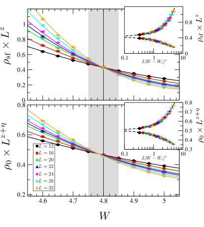
The ordered regime is characterized by a finite SF density , efficiently estimated using the winding number fluctuations in the QMC algorithm Pollock and Ceperley (1987). In the vicinity of the 2D quantum critical point, the finite-size scaling of the SF density is
| (2) |
where is the dynamical critical exponent, the correlation length exponent, the critical disorder, and a universal function.
Beyond the SF response, one can also probe Bose-Einstein condensation (BEC), occurring in 2D at where U(1) symmetry can be broken. The BEC density , obtained from the equal time Green’s function Dorneich and Troyer (2001) , plays the role of the order parameter, with a critical scaling
| (3) |
Our QMC data are very nicely described by the above scaling forms, as shown in Fig. 1 for both SF and BEC densities. Strikingly, BEC and SF densities vanish at the same disorder strength . The values of the critical exponents are given in Table 1. This determination results from fits of our data set by Taylor expanding the scaling functions and around up to an order large enough that the goodness of fit is acceptable (3rd order in Fig. 1, see sm ). We have performed a careful error analysis using the bootstrap approach in order to estimate statistical errors of the fit parameters, as well as potential systematic errors by fitting over various ranges of disorder strengths and sizes sm . This results in conservative uncertainties for the estimates of the critical parameters, as visible in Tab. 1.
We observe a good agreement with the predicted bounds from Fisher et al. Fisher et al. (1989) for and . Regarding the more debated question of the dynamical exponent Weichman and Mukhopadhyay (2007), while still compatible with within error bars our best estimate gives a smaller number , in agreement with a recent careful estimate for quantum rotors Meier and Wallin (2012). Comparing with other studies in Tab. 1, our results, obtained with much larger system sizes, agree within error bars with Ref. Zhang et al. (1995), whereas results in Refs. Makivić et al. (1993); Priyadarshee et al. (2006) are probably biased due to finite temperature effects and too small disorder averaging.

Distributions and absence of self-averaging in the BG— In order to go beyond the analysis of the critical properties based on disorder averaged observables, we now turn to the much less studied issue of distributions. The question of a possible broadening of the responses, linked to the issue of self-averaging, has not been studied for 2D bosons, although it may be crucial as discussed for disordered Ising models Fisher (1995); Young and Rieger (1996); Wiseman and Domany (1998) and strongly disordered superconductors Feigel’man et al. (2010); Sacépé et al. (2011); Lemarié et al. (2013). Here we focus on the probability distribution , obtained by building histograms of QMC estimates for over independent samples, with for and for , shown in Fig. 2 for three values of the disorder strength.
In the SF regime (panel (a) ) the distribution narrows upon increasing the size , thus demonstrating that the SF response is self-averaging in the ordered phase. Conversely, as visible in panel (d) for the BG regime at , broadens when increases, and moves towards large negative values, as expected in the thermodynamic limit where the SF stiffness vanishes. We therefore expect a difference between average and typical SF densities in the BG: as shown in the insets of Fig. 2, the ratio clearly increases with in the BG regime (d) whereas it goes to 1 in the SF phase (a). At the critical point (panels (b-c) of Fig. 2), the histograms first broaden for small sizes and then, above the curves appear self-similar, simply shifted relative to each other. This absence of broadening at large scales is also visible in the inset (b) where the ratio tends to saturate to a constant value. The shift of the distributions can be corrected for by adding to using our best estimate . Indeed, as shown in Fig. 2 (c) yields a collapse onto a scale invariant distribution, particularly good above .
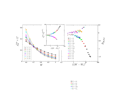
The fact that all distributions at are identical up to a shift suggests that, while typical and average SF densities scale differently in the BG regime, their critical scalings are described by the same exponents. Indeed, the typical SF density, defined as (where stands for disorder averaging), can be analyzed using a scaling hypothesis similar to the average Eq. (2), but including additional irrelevant corrections Rodriguez et al. (2011)
| (4) |
Because of the presence of irrelevant corrections, a fit of our data set by Eq. (4) with a polynomial is unstable unless we fix the critical parameters , and to our best estimates (Tab. 1). The crossing of vs plotted in Fig. 3 (a) displays a non-negligible drift, well captured by irrelevant corrections in Eq. (4) with . A nice way to achieve a scaling plot for the typical SF density is then to divide by its value at , this in order to cancel out the irrelevant corrections . Next, a rescaling of the length by the correlation length with and , gives an almost perfect collapse, without any additional adjustable parameters, as shown in Fig. 3 (b) for and all available system sizes . This demonstrates that the quantum critical behaviours of average and typical SF densities are similar, in particular their critical exponents and .
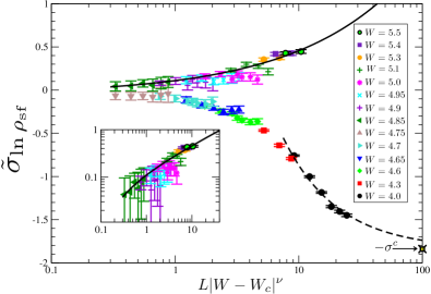
Coming back to the distributions, the drift observed for the typical stiffness in Fig. 3 (a) is related to the transient (irrelevant) broadening of observed at small sizes in Fig. 2 (b). In order to take such a crossover into account and get rid of irrelevant corrections, we study the broadening of using the corrected standard deviation (StD) , where is the StD at criticality. This is plotted in Fig. 4 vs. , where a very good collapse of the data is achieved without any adjusted parameters. In the SF regime, converges towards as (dashed curve), a consequence of self-averaging. More interestingly, the BG phase features an opposite qualitative behavior with growing with system size, as (full line). A careful study of such very broad distributions hits the limits of our numerics, leading to quite large statistical errors, despite the very large number of samples , but nevertheless allows to estimate the exponent . We interpret this result as follows: The prediction Seibold et al. (2012a) that the stiffness is dominated by quasi 1D paths suggests that one may understand the global SF response as a purely local quantity in the BG insulator. Moreover, an analogy Feigel’man et al. (2010); Lemarié et al. (2013) between the BG and the disordered phase of the random transverse-field Ising model Fisher (1995), as supported by recent 1D results Javan Mard et al. (2014), suggests that the BG is governed by directed-polymer physics in dimension Monthus and Garel (2012). This predicts an exponent Huse et al. (1985) for local quantities which is compatible with our estimate.
Local density and absence of percolation— Finally, we want to discuss some microscopic properties of the insulating BG state. For this we focus on the local bosonic density , shown in Fig. 5 in the BG regime () for , at low enough temperature such that the total number of bosons does not fluctuate (see sm ).
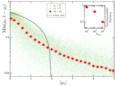
Clearly, the average behavior is
always compressible, which contrasts with the clean case where the system is incompressible whenever Coletta et al. (2012). Furthermore, the
fraction of incompressible sites with or decreases with the number of MC steps
and seems to vanish in the exact limit (inset). This shows that percolation through
compressible sites is present even in the BG phase, at least from such a single particle view, and is therefore not related to the SF-BG transition, in contrast with some recent discussions Niederle and Rieger (2013); Krinner et al. (2013b).
Conclusions— Large-scale QMC simulations of the SF-BG transition supplemented by finite-size scaling show that SF and BEC densities disappear at the same critical disorder strength , with critical exponents , , and . The SF density distribution becomes infinitely broad upon increasing system size in the BG insulator, a characteristic signature of the absence of self-averaging supporting the fact that the SF density is a purely local quantity at strong disorder. Our results also rule out a classical percolation scenario of incompressible sites in the BG.
This work was performed using HPC
resources from GENCI (grant x2014050225) and CALMIP (grant 2014-P0677), and is supported by the
French ANR program ANR-11-IS04-005-01 and by the label NEXT. During the completion of this study we became aware of a parallel work eri , which reaches comparable conclusions.
References
- Giamarchi (2013) T. Giamarchi, Comptes Rendus Physique 14, 637 (2013).
- Finotello et al. (1988) D. Finotello, K. A. Gillis, A. Wong, and M. H. W. Chan, Phys. Rev. Lett. 61, 1954 (1988).
- Reppy (1992) J. D. Reppy, J Low Temp Phys 87, 205 (1992).
- Ma and Lee (1985) M. Ma and P. A. Lee, Phys. Rev. B 32, 5658 (1985).
- Ma et al. (1986) M. Ma, B. I. Halperin, and P. A. Lee, Phys. Rev. B 34, 3136 (1986).
- Giamarchi and Schulz (1987) T. Giamarchi and H. J. Schulz, EPL 3, 1287 (1987).
- Fisher and Fisher (1988) D. S. Fisher and M. P. A. Fisher, Phys. Rev. Lett. 61, 1847 (1988).
- Fisher et al. (1989) M. P. A. Fisher, P. B. Weichman, G. Grinstein, and D. S. Fisher, Phys. Rev. B 40, 546 (1989).
- Josephson (1966) B. D. Josephson, Physics Letters 21, 608 (1966).
- Krauth et al. (1991) W. Krauth, N. Trivedi, and D. Ceperley, Phys. Rev. Lett. 67, 2307 (1991).
- Scalettar et al. (1991) R. T. Scalettar, G. G. Batrouni, and G. T. Zimanyi, Phys. Rev. Lett. 66, 3144 (1991).
- Sørensen et al. (1992) E. S. Sørensen, M. Wallin, S. M. Girvin, and A. P. Young, Phys. Rev. Lett. 69, 828 (1992).
- Makivić et al. (1993) M. Makivić, N. Trivedi, and S. Ullah, Phys. Rev. Lett. 71, 2307 (1993).
- Weichman (1995) P. B. Weichman, Phys. Rev. Lett. 74, 1038 (1995).
- Zhang et al. (1995) S. Zhang, N. Kawashima, J. Carlson, and J. E. Gubernatis, Phys. Rev. Lett. 74, 1500 (1995).
- Kisker and Rieger (1997) J. Kisker and H. Rieger, Phys. Rev. B 55, R11981 (1997).
- Alet and Sørensen (2003) F. Alet and E. S. Sørensen, Phys. Rev. E 67, 015701 (2003).
- Prokof’ev and Svistunov (2004) N. Prokof’ev and B. Svistunov, Phys. Rev. Lett. 92, 015703 (2004).
- Priyadarshee et al. (2006) A. Priyadarshee, S. Chandrasekharan, J.-W. Lee, and H. U. Baranger, Phys. Rev. Lett. 97, 115703 (2006).
- Hitchcock and Sørensen (2006) P. Hitchcock and E. S. Sørensen, Phys. Rev. B 73, 174523 (2006).
- Gurarie et al. (2009) V. Gurarie, L. Pollet, N. V. Prokof’ev, B. V. Svistunov, and M. Troyer, Phys. Rev. B 80, 214519 (2009).
- Carrasquilla et al. (2010) J. Carrasquilla, F. Becca, A. Trombettoni, and M. Fabrizio, Phys. Rev. B 81, 195129 (2010).
- Lin et al. (2011) F. Lin, E. S. Sørensen, and D. M. Ceperley, Phys. Rev. B 84, 094507 (2011).
- Söyler et al. (2011) S. Söyler, M. Kiselev, N. V. Prokof’ev, and B. V. Svistunov, Phys. Rev. Lett. 107, 185301 (2011).
- Meier and Wallin (2012) H. Meier and M. Wallin, Phys. Rev. Lett. 108, 055701 (2012).
- Yao et al. (2014) Z. Yao, K. P. C. da Costa, M. Kiselev, and N. Prokof’ev, Phys. Rev. Lett. 112, 225301 (2014).
- Pai et al. (1996) R. V. Pai, R. Pandit, H. R. Krishnamurthy, and S. Ramasesha, Phys. Rev. Lett. 76, 2937 (1996).
- Rapsch et al. (1999) S. Rapsch, U. Schollwöck, and W. Zwerger, EPL 46, 559 (1999).
- Roux et al. (2008) G. Roux, T. Barthel, I. McCulloch, C. Kollath, U. Schollwöck, and T. Giamarchi, Phys. Rev. A 78, 023628 (2008).
- Singh and Rokhsar (1992) K. G. Singh and D. S. Rokhsar, Phys. Rev. B 46, 3002 (1992).
- Herbut (1997) I. F. Herbut, Phys. Rev. Lett. 79, 3502 (1997).
- Weichman and Mukhopadhyay (2007) P. B. Weichman and R. Mukhopadhyay, Phys. Rev. Lett. 98, 245701 (2007).
- Altman et al. (2010) E. Altman, Y. Kafri, A. Polkovnikov, and G. Refael, Phys. Rev. B 81, 174528 (2010).
- Ristivojevic et al. (2012) Z. Ristivojevic, A. Petković, P. Le Doussal, and T. Giamarchi, Phys. Rev. Lett. 109, 026402 (2012).
- Iyer et al. (2012) S. Iyer, D. Pekker, and G. Refael, Phys. Rev. B 85, 094202 (2012).
- Álvarez Zúñiga and Laflorencie (2013) J. P. Álvarez Zúñiga and N. Laflorencie, Phys. Rev. Lett. 111, 160403 (2013).
- White et al. (2009) M. White, M. Pasienski, D. McKay, S. Q. Zhou, D. Ceperley, and B. DeMarco, Phys. Rev. Lett. 102, 055301 (2009).
- Deissler et al. (2010) B. Deissler, M. Zaccanti, G. Roati, C. D’Errico, M. Fattori, M. Modugno, G. Modugno, and M. Inguscio, Nat Phys 6, 354 (2010).
- Krinner et al. (2013a) S. Krinner, D. Stadler, J. Meineke, J.-P. Brantut, and T. Esslinger, Phys. Rev. Lett. 110, 100601 (2013a).
- D’Errico et al. (2014) C. D’Errico, E. Lucioni, L. Tanzi, L. Gori, G. Roux, I. P. McCulloch, T. Giamarchi, M. Inguscio, and G. Modugno, Phys. Rev. Lett. 113, 095301 (2014).
- Sacépé et al. (2011) B. Sacépé, T. Dubouchet, C. Chapelier, M. Sanquer, M. Ovadia, D. Shahar, M. Feigel’man, and L. Ioffe, Nat Phys 7, 239 (2011).
- Lemarié et al. (2013) G. Lemarié, A. Kamlapure, D. Bucheli, L. Benfatto, J. Lorenzana, G. Seibold, S. C. Ganguli, P. Raychaudhuri, and C. Castellani, Phys. Rev. B 87, 184509 (2013).
- Driessen et al. (2012) E. Driessen, P. Coumou, R. Tromp, P. de Visser, and T. Klapwijk, Phys. Rev. Lett. 109, 107003 (2012).
- Mondal et al. (2013) M. Mondal, A. Kamlapure, S. C. Ganguli, J. Jesudasan, V. Bagwe, L. Benfatto, and P. Raychaudhuri, Sci. Rep. 3 (2013).
- Hong et al. (2010) T. Hong, A. Zheludev, H. Manaka, and L.-P. Regnault, Phys. Rev. B 81, 060410 (2010).
- Hüvonen et al. (2012) D. Hüvonen, S. Zhao, M. Månsson, T. Yankova, E. Ressouche, C. Niedermayer, M. Laver, S. N. Gvasaliya, and A. Zheludev, Phys. Rev. B 85, 100410 (2012).
- Yu et al. (2012) R. Yu, L. Yin, N. S. Sullivan, J. S. Xia, C. Huan, A. Paduan-Filho, N. F. Oliveira Jr, S. Haas, A. Steppke, C. F. Miclea, F. Weickert, R. Movshovich, E.-D. Mun, B. L. Scott, V. S. Zapf, and T. Roscilde, Nature 489, 379 (2012).
- Vojta (2013) M. Vojta, Phys. Rev. Lett. 111, 097202 (2013).
- Zheludev and Roscilde (2013) A. Zheludev and T. Roscilde, Comptes Rendus Physique 14, 740 (2013).
- Feigel’man et al. (2010) M. V. Feigel’man, L. B. Ioffe, and M. Mézard, Phys. Rev. B 82, 184534 (2010).
- Krinner et al. (2013b) S. Krinner, D. Stadler, J. Meineke, J.-P. Brantut, and T. Esslinger, arXiv:1311.5174 (2013b).
- Hegg et al. (2013) A. Hegg, F. Krüger, and P. W. Phillips, Phys. Rev. B 88, 134206 (2013).
- Weichman and Mukhopadhyay (2008) P. B. Weichman and R. Mukhopadhyay, Phys. Rev. B 77, 214516 (2008).
- Seibold et al. (2012a) G. Seibold, L. Benfatto, C. Castellani, and J. Lorenzana, Phys. Rev. Lett. 108, 207004 (2012a).
- Syljuåsen and Sandvik (2002) O. F. Syljuåsen and A. W. Sandvik, Phys. Rev. E 66, 046701 (2002).
- (56) See supplementary Material.
- Sandvik (2002) A. W. Sandvik, Phys. Rev. B 66, 024418 (2002).
- Laflorencie et al. (2006) N. Laflorencie, S. Wessel, A. Läuchli, and H. Rieger, Phys. Rev. B 73, 060403 (2006).
- Pollock and Ceperley (1987) E. Pollock and D. Ceperley, Phys. Rev. B 36, 8343 (1987).
- Dorneich and Troyer (2001) A. Dorneich and M. Troyer, Phys. Rev. E 64, 066701 (2001).
- Fisher (1995) D. S. Fisher, Phys. Rev. B 51, 6411 (1995).
- Young and Rieger (1996) A. P. Young and H. Rieger, Phys. Rev. B 53, 8486 (1996).
- Wiseman and Domany (1998) S. Wiseman and E. Domany, Phys. Rev. Lett. 81, 22 (1998).
- Rodriguez et al. (2011) A. Rodriguez, L. J. Vasquez, K. Slevin, and R. A. Römer, Phys. Rev. B 84, 134209 (2011).
- Javan Mard et al. (2014) H. Javan Mard, J. A. Hoyos, E. Miranda, and V. Dobrosavljević, Phys. Rev. B 90, 125141 (2014).
- Monthus and Garel (2012) C. Monthus and T. Garel, Journal of Physics A: Mathematical and Theoretical 45, 095002 (2012).
- Huse et al. (1985) D. Huse, C. Henley, and D. Fisher, Phys. Rev. Lett. 55, 2924 (1985).
- Coletta et al. (2012) T. Coletta, N. Laflorencie, and F. Mila, Phys. Rev. B 85, 104421 (2012).
- Niederle and Rieger (2013) A. E. Niederle and H. Rieger, New Journal of Physics 15, 075029 (2013).
- (70) R. Ng and E. S. Sørensen (preprint).
Appendix A SUPPLEMENTARY MATERIAL
This supplementary material provides additional information about our results and details the simulation and data analysis methods. We discuss in detail how finite temperature QMC results are used to access ground-state information, how we perform our careful error analysis and how we extract our best estimates for the critical exponents of the transition. We also analyze the problem of large autocorrelation times for the superfluid density in the Bose glass phase.
Appendix B I. -DOUBLING SCHEME AND GROUND-STATE CONVERGENCE
The stochastic series expansion (SSE) being a finite temperature method, it is important to perform calculations at low enough temperatures to capture ground state (GS) properties. In order to accurately study this GS convergence, we have used the -doubling scheme sandvik_classical_2002_sm which consists in performing simulations at exponentially decreasing temperatures by doubling the inverse temperature as long as we still see a change of the disorder average between the two previous temperatures.
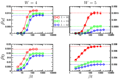
This -doubling trick allows us to determine the inverse temperature at which we should perform the simulations for every system size and every disorder strength in order to ensure that we are really investigating the GS properties. In Fig. 6 we show for two disorder strengths: in the superfluid (SF) and in the Bose glass (BG) results of -doublings for SF and BEC densities, both averaged over random samples for three system sizes (). We nicely see that GS-converged expectation values are reached when saturation is achieved. From this -doubling study, we have fixed for the production simulations for and up to for to study the quantum () superfluid - Bose glass phase transition.
It is worth noticing that in the right panel of Fig. 6 we also show the -doubling data for and with a bigger number of MC steps, , which are in perfect agreement with the results for . This feature will be further discussed below.
Note that the -doubling scheme can be implemented efficiently in SSE by replicating (and inverting) the operator string at inverse temperature to obtain an operator string twice as long as an efficient starting point at the inverse temperature , thus minimizing the equilibration time of the Markov chain at . This method is also used to speed up the thermalization process for all our production runs.
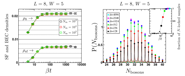
Nevertheless, the notion of GS convergence appears to be quite subtle when monitoring various observables. Indeed, the temperature at which a given disordered sample is effectively in its GS, i.e. below the finite size gap, is strongly tied to the disorder realization, and contributions from low energy excited states depend on the physical observable which is measured. For example, the total number of particles is a good quantum number and therefore has to be locked in the GS to an integer number. In the Bose glass (BG) regime, where very small finite size gaps are expected, the histogram of obtained over several hundreds of samples slowly evolves when varying the temperature towards a collection of -peaks, but only for very large , as shown in Fig. 7 (right panel). Interestingly, the fraction of samples that are not fully converged to their GS (inset of Fig. 7 right), as far as the total number of bosons is concerned, remain sizeable while the disorder average superfluid (SF) or Bose-Einstein condensate (BEC) densities appear well converged to their values, as shown in the left panel of Fig. 7. There we see that for , the average SF and BEC densities appear converged in temperature for while the actual fraction of samples with locked is less than 30% for .
BEC and SF densities converge much faster to their values than . This undoubtedly facilitates the GS simulations as we can stop the cooling procedure at not too large inverse temperature, as far as SF and BEC densities are concerned. Nevertheless, one should still pay attention to potential systematic bias that may be introduced by rare disorder realizations that may have not fully converged to their GS values for and . To do so, we fit the -doubling curves of as a function of temperature to the following form
| (5) |
which turns out to describe quite well our results with the following fitting parameters
| (6) |
With this simple phenomenological description, we have checked the stability of our scaling analysis, and concluded that our results do not change upon the inclusion of such a correction term (see Fig. 12). Note that the correction is small enough so that the corrected result is still within the error bar as guaranteed by our convergence check in Fig. 6.
Appendix C II. ERROR BARS AND EVALUATION OF SYSTEMATIC ERRORS
Monte Carlo (MC) results for disordered systems have two sources of statistical errors: (i) Statistical fluctuations of the Monte Carlo result for each random sample, which can be reduced by generating longer Markov chains. (ii) Statistical fluctuations of the disorder average over random samples which can be reduced by including more realizations.
C.1 A. MC error vs. disorder fluctuations
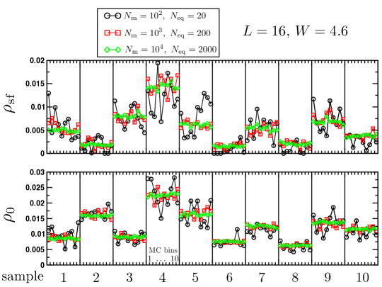
It is crucial to distribute the available computer time efficiently over the different competing tasks (large , number of MC steps, number of random samples) in order to maximize the overall precision. Therefore, we compare the MC error bar to the error bar stemming from disorder averaging. We choose a minimal number of 1000 MC measurements in order to assure that the Markov chain is much longer than the autocorrelation times of and and it is not allowed to perform less MC steps as this leads to wrong results and introduces a systematic error.
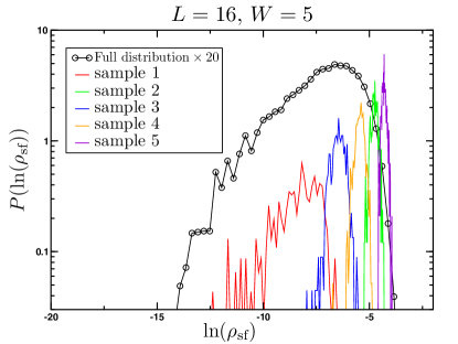
Figure 8 shows clearly that MC fluctuations within one disorder realization are much smaller than the error bar stemming from the fluctuations between disorder realizations. Indeed, we see that while MC fluctuations with are of the same order of magnitude that sample-to-sample fluctuations, making measurement steps is enough to keep MC errors much smaller than fluctuations due to random configurations.To further illustrate in a more quantitative way the fact that disorder fluctuations are much bigger than MC fluctuations, we show in Fig. 9 the full distribution of obtained for a system of linear size with samples at disorder strength (BG regime) on which we have superimposed histograms of MC averages over MC steps for 5 representative samples. Hence, it appears more efficient to perform a relatively modest number of MC steps , in order to be able to sample more disorder realizations. Note that the MC error is nevertheless included in our data analysis as discussed below.
C.2 B. Disorder fluctuations
The problem of increasing variances in the BG phase leads to a sampling issue which can be tackled for finite systems by using a very large number of disorder realizations. In order to estimate how many samples should be used to obtain a reliable and converged result, we calculate running means as a function of the number of disorder realizations.
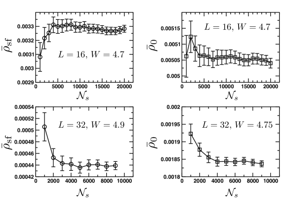
Figure 10 shows the estimated averages and error bars of both SF and BEC densities for increasing number of disorder realizations for different system sizes and disorder strengths. Seemingly, averages over around 1000 disorder realizations are not fully converged and for the smaller system sizes, at least some 10000 disordered samples are needed for a converged result, while for larger systems, at least 5000 disordered samples are required. To be safe, we choose to reach 20000 disorder realizations for the smaller sizes and 10000 for system sizes .
In addition, a very large number of disorder realizations are also needed to correctly sample the distributions of since they broaden with increasing system size, as shown in the main text. This further justifies our choice of such very large numbers of samples (see also Ref. lin_superfluid-insulator_2011_sm for a related discussion).
C.3 C. Bootstrap analysis
For our scaling analysis of and it is crucial to take into account the correct error bars of our results for every system size and disorder strength. While the average value is simply given by the disorder average of the MC averages, the total error bar can be estimated using a bootstrap approach. For this, we generate a set of bootstrap samples by randomly selecting a subset from the realizations with replacement (selecting in total realizations from the ensemble with replacement) and drawing a Gaussian random number distributed according to
| (7) |
for each selected sample, which we then average over . This is repeated many (typically ) times and the standard deviation of the result is indeed an accurate estimator of the total error bar. We have also checked that the MC error is smaller than the disorder fluctuations so that the final results are unchanged if it is neglected (see Fig. 12).
In order to determine error bars of the critical disorder strength and the critical exponents, a second level of bootstrap analysis is introduced, which performs multiple fits by a gaussian resampling of our results for and within the previously determined error bars. The standard deviation of the such obtained fit results represent the statistical error of the final results (see Fig. 12 and table 2)
Appendix D III. OVERCOMING LARGE AUTOCORRELATION TIMES FOR
D.1 A. Dynamical increase of the number of MC steps
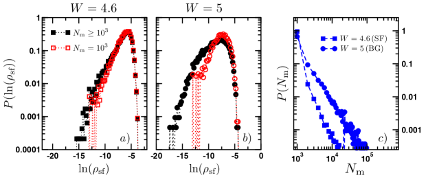
For disorder realizations which exhibit a particularly small value of the superfluid density , which is measured in the SSE by counting the winding number fluctuation of worldlines, we find that autocorrelation times become larger and the change between the winding number sector to nonzero winding numbers takes more MC steps. For these cases, we decide dynamically to perform additional blocks of 1000 MC steps until the final result is reliable and the total simulation time is much longer than the autocorrelation time, involving simulations with up to MC steps. This method gives reliable access to small values of , which would be estimated to be otherwise, which is not expected for our finite size samples.
We set the MC steps limit for computing time reasons and the rare disorder realizations needing more steps are evaluated to zero stiffness. These realizations cannot be used for the discussion on the distributions of , nor the typical stiffness. However, they can be included in the calculation of the average stiffness as neglecting them would induce systematic errors. In fact, our analysis leads us to speculate that these samples have been simulated at a too high temperature and are not converged to the GS.
There are several possibilities which we all explored and found little dependence of our results on
the particular choice.
i) Adding samples of vanishing to the data set and performing the data analysis
described before. This corresponds to approximating the distribution of by a
distribution with a cut-off at the minimal stiffness observed in the ensemble and a delta peak at
zero. Clearly this is an incorrect estimation as the correct distribution vanishes at zero and the
delta peak is both due to insufficient simulation time and too high temperature, thus introducing a
(small) systematic error.
ii)
Extrapolation of the distributions of towards zero by a power law tail (straight line in the plots in figure 11)
but since this is the least properly sampled part of the distribution a reliable extrapolation cannot be achieved.
iii) The replacement of the non physical zero values by half the value of the cut-off (i.e. the minimal computed stiffness for every
couple ). This corresponds to approximating
the small tail of the distribution by a box distribution and is only justified by
the very small weight of the approximated part of the distribution.
We used this last solution for checking the stability of our scaling analysis and found that our results
are not dependent on whether these samples are included or not.
Hence, to treat on equal footing the typical and average stiffness, we decided
to neglect them, as the introduced bias is much smaller than our overall uncertainty.
Future work could try to adress this problem by investing more computer time in samples with small values of . We have found that these samples are typically not completely converged in the GS and it should be explored if one can solve the problem by reducing the temperature iteratively in such samples.
D.2 B. Improved sampling of the full stiffness distributions
A comparison of results obtained
with only fixed to MC steps to results obtained with our dynamic Markov chain
length method are displayed in Fig. 11 for a system in the SF (though
strongly disordered) regime (panel ) and inside the BG phase (panel ). It is clear that our
dynamical adjustment of the MC steps allows for much smaller SF stiffnesses to be computed,
especially inside the BG phase. The implementation of this procedure allows for the
distribution of to be accurately sampled and hence, for an appropriate
estimation of the standard deviation of . Without this method, the broadening
of the distributions for growing system sizes inside the BG phase (described in the main text)
could not have been investigated quantitatively, nor even qualitatively observed.
Appendix E IV. CRITICAL EXPONENTS
| () | () | |||||
|---|---|---|---|---|---|---|
| 8.7 | 13.3 | 16.2 | 4.5 | 4.25 | 11 | |
| 7 | 15.2 | 13.5 | 4 | 5 | 9.2 | |
| 21.3 | 39.75 | 33.8 | 37.5 | 39.25 | 39.5 | |
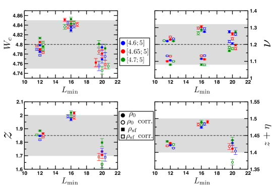
We have discussed above how the statistical error on the critical disorder strength and the critical exponents may be obtained. However, we believe that the systematic error due to small system sizes which may require corrections to scaling in our scaling analysis is in fact dominant, as results change slightly if the size of the fit window in system size or included disorder strengths is varied.
Therefore, we have performed a systematic analysis of this systematic error and give error bars that represent the total fluctuation of our results. This is represented in Fig. 12.
In order to quantify the quality of our fits, we calculate the sum of squared residuals
| (8) |
and obtain the probability of finding a greater or equal than this value given the fit by
| (9) |
as explained in Ref. young_everything_2012, .
The corresponding qualities of fit for each window in size and included disorder strengths are shown in table 2. There are two reasons why the qualities of fit are systematically larger for the window . First, reducing the number of system sizes included in the analysis while keeping the bigger sizes means that there is less size dynamics, hence the fact that no drift term is included in the fits becomes more justified. Secondly, the bigger system sizes have slightly bigger relative error bars so the corresponding is smaller and the quality of fit larger as these two quantities are very sensible to the error bars. Consequently, we treat all fit windows on equal footing to estimate averages and uncertainties and do not give a bigger weight to the estimates obtained with .
In figure 12 we plot the critical parameters with their error bars, obtained from a bootstrap analysis with 100 bootstrap samples, for every window in system size and included disorder strength corresponding to table 2. For comparison, the critical exponents and critical disorder strength estimates, with their error bars, given upon including the corrections to the systematic errors due to temperature convergence and the Monte Carlo error bars are also shown (open symbols). It is clear that including the correction of the possible systematic errors does not change the final estimations of the critical parameters as well as their error bars, which are quite large.
References
- (1) A. W. Sandvik Phys. Rev. B 66, 024418 (2002).
- (2) F. Lin, E. S. Sørensen, and D. M. Ceperley, Phys. Rev. B 84, 094507 (2011).
- (3) P. Young, arXiv e-print 1210.3781 (2012).