Scaling properties of one-dimensional driven-dissipative condensates

Abstract

We numerically investigate the scaling properties of a one-dimensional driven-dissipative condensate described by a stochastic complex Ginzburg-Landau equation (SCGLE). We directly extract the static and dynamical scaling exponents from the dynamics of the condensate’s phase field, and find that both coincide with the ones of the one-dimensional Kardar-Parisi-Zhang (KPZ) equation. We furthermore calculate the spatial and the temporal two-point correlation functions of the condensate field itself. The decay of the temporal two-point correlator assumes a stretched-exponential form, providing further quantitative evidence for an effective KPZ description. Moreover, we confirm the observability of this non-equilibrium scaling for typical current experimental setups with exciton-polariton systems, if cavities with a reduced $Q$ factor are used.

I Introduction

Physical systems driven far away from thermal equilibrium can show intrinsically different properties from their equilibrium counterparts. One prototypical example is the growing interface, whose long-wavelength dynamics, described by the so-called Kardar-Parisi-Zhang (KPZ) equation KPZ_equation , does not belong to the Halperin-Hohenberg classification of near thermal equilibrium dynamical behavior HH_models . Recent experimental progress in realizing Bose-Einstein condensation of exciton-polaritons in pumped semiconductor heterostructures Polariton_Experiment_1 ; Polariton_Experiment_2 ; Polariton_Experiment_3 holds the promise of developing such systems into laboratories for non-equilibrium statistical mechanics. Microscopically, these systems exhibit coherent and driven-dissipative dynamics on an equal footing, and therefore explicitly violate detailed balance characteristic of an equilibrium system. This phenomenology can have drastic consequences for the macrophysics of such systems. Indeed, for the case of driven-dissipative condensates of exciton-polaritons in two dimensions (2D), it was pointed out recently Altman_2d_driven_SF_2013 that quasi-long-range order can not exist in the long-wavelength limit, in stark contrast to the familiar properties of 2D equilibrium condensates. This conclusion was drawn from a connection between the stochastic complex Ginzburg-Landau equation (SCGLE) and the KPZ equation in the long-wave length limit Grinstein_KPZ_SCGLE ; Altman_2d_driven_SF_2013 , as also noticed in 1D Wouters_1D_static . However, direct numerical evidence of this connection is still missing.

As a first step to fill this gap, here we investigate the long-wavelength behavior of the dynamics of a driven-dissipative condensate in 1D. Our first goal is to study whether scaling properties of the condensate’s phase field dynamics, in particular static and dynamical exponents, indeed coincide with those implied by the KPZ equation. The second goal is to directly study both the spatial and temporal correlation function of the bosonic field for the condensate itself to see whether they match the prediction from the KPZ picture. We note that a similar investigation is reported in Wouters_1d_temproal , and comment on the relation to the present work in Sec. IV.

We achieve our goals via direct numerical simulations of the SCGLE which governs the dynamics of driven-dissipative condensates. We directly extract both the static and dynamical critical exponents of the system from the dynamics of the condensate’s phase field. Within numerical error, we indeed find that the critical exponents of the SCGLE coincide with the ones of the KPZ equation (see Figs. 1, 5, and 6), and we estimate the crossover time scale (see Fig. 2) beyond which the KPZ scaling behavior can be observed. We further find that the scaling properties of the condensate field dynamics (see Figs. 3 and 4) match the expectation from the effective description in terms of the KPZ equation. Finally, we demonstrate that the KPZ scaling can be seen in current experimental setups with exciton-polaritons, if cavities with a reduced $Q$ factor are used (see Fig. 4).

Our numerical approach is based on an effective lower polariton dynamical model with a quartic nonlinearity. Another widely used dynamical model for exciton-polariton condensates is the so-called generalized Gross-Pitaevskii equation Carusotto2013 ; Wouters_1D_static ; Wouters_1d_temproal , which results from a two-band model after tracing out the reservoir band Carusotto2013 . As a matter of fact these two models coincide with each other after expanding the nonlinear term in the generalized Gross-Pitaevskii equation with respect to the polariton field (see for instance Eq. (14)). We note that KPZ scaling behavior only emerges at long wavelengths, where general power counting arguments ensure that this approximation (with low order in the polariton fields) is well justified in the long wavelength limit.

The paper is organized as follows: In Sec. II, we specify the system and model under study, and the theoretical approach used. In Sec. III, we present a detailed discussion of the scaling properties of the phase field correlations. This contains in particular the static and dynamical exponents of the condensate’s phase field dynamics. In Sec. IV, we discuss the scaling properties of two-point correlation functions of the condensate field itself. In Sec. V, we investigate the experimental observability of the scaling properties discussed in Sec. IV in exciton-polariton condensate experiments. We conclude and give an outlook in Sec. VI.

II Model and Theoretical Approach

The dynamics of driven-dissipative condensates, which have been realized in experiments with exciton-polariton systems Polariton_Experiment_2 ; Polariton_Experiment_3 ; Polariton_Experiment_1 , can be modeled by the SCGLE with a complex Gaussian white noise (units are chosen such that $\hbar=1$) which reads in 1D as Carusotto2013 ; Altman_2d_driven_SF_2013

$$\frac{\partial}{\partial\tilde{t}}\tilde{\psi}=\left[\tilde{r}+\tilde{K}\frac{\partial^{2}}{\partial\tilde{x}^{2}}+\tilde{u}|\tilde{\psi}|^{2}\right]\tilde{\psi}+\tilde{\zeta}$$ (1)

with $\tilde{r}=-\tilde{r}_{d}-i\tilde{r}_{c}$, $\tilde{K}=\tilde{K}_{d}+i\tilde{K}_{c}$, $\tilde{u}=-\tilde{u}_{d}-i\tilde{u}_{c}$, $\langle\tilde{\zeta}(\tilde{x},\tilde{t})\tilde{\zeta}(\tilde{x}^{\prime},\tilde{t}^{\prime})\rangle=0$, $\langle\tilde{\zeta}^{*}(\tilde{x},\tilde{t})\tilde{\zeta}(\tilde{x}^{\prime},\tilde{t}^{\prime})\rangle=2\tilde{\sigma}\delta(\tilde{x}-\tilde{x}^{\prime})\delta(\tilde{t}-\tilde{t}^{\prime})$. The second moment of the noise $\tilde{\sigma}=\tilde{\gamma}_{l}$ with $\tilde{\gamma}_{l}$ being the single particle loss, while $\tilde{r}_{d}=\tilde{\gamma}_{l}-\tilde{\gamma}_{p}$ is the difference between the single particle loss and pump. For the existence of a condensate in the mean field steady state solution, $\tilde{r}_{d}$ has to be negative, i.e., the single-particle pump rate has to be larger than the loss rate. $\tilde{u}_{d}$ is the positive two-particle loss rate; $K_{c}=1/(2m_{\mathrm{LP}})$ with $m_{\mathrm{LP}}$ being the mass of polaritons and $K_{d}$ is an effective diffusion constant. For convenience, we use the following rescaled form of Eq. (1),

$$\frac{\partial}{\partial t}\psi = \left[r+K\frac{\partial^{2}}{\partial x^{2}}+u|\psi|^{2}\right]\psi+\zeta,$$ (2)

where

$$t=|\tilde{r}_{d}|\tilde{t},\,x=\sqrt{\frac{|\tilde{r}_{d}|}{\tilde{K}_{d}}}\tilde{x},$$ (3)

$$\psi=\sqrt{\frac{\tilde{u}_{d}}{|\tilde{r}_{d}|}}\tilde{\psi},\,\zeta=\sqrt{\frac{\tilde{u}_{d}}{|\tilde{r}_{d}|^{3}}}\tilde{\zeta},$$ (4)

$$r_{c}=\frac{\tilde{r}_{c}}{|\tilde{r}_{d}|},\,K_{c}=\frac{\tilde{K}_{c}}{\tilde{K}_{d}},\,u_{c}=\frac{\tilde{u}_{c}}{\tilde{u}_{d}},$$ (5)

$$r=1-ir_{c},\,K=1+iK_{c},\,u=-1-iu_{c},$$ (6)

and the second moment of the rescaled Gaussian white noise $\zeta(x,t)$ is $\sigma=\tilde{\sigma}\tilde{u}_{d}\left|\tilde{r}_{d}\right|^{-3/2}\tilde{K}_{d}^{-1/2}$.

Adopting the amplitude-phase representation of the complex bosonic field $\psi(x,t)=\rho(x,t)e^{i\theta(x,t)}$, it was shown Grinstein_KPZ_SCGLE ; Altman_2d_driven_SF_2013 ; Wouters_1D_static that, assuming that spatial-temporal fluctuations of the amplitude field $\rho(x,t)$ are small, the dynamical equation of the phase field $\theta(x,t)$ assumes in the low-frequency and long-wavelength limit the form of the KPZ equation, which reads

$$\partial_{t}\theta(x,t)=D\partial_{x}^{2}\theta(x,t)+\frac{\lambda}{2}\left(\partial_{x}\theta(x,t)\right)^{2}+\eta(x,t),$$ (7)

where $\eta(x,t)$ is an effective Gaussian white noise, with mean $\langle\eta(x,t)\rangle=0$, and correlations $\langle\eta(x,t)\eta(x^{\prime},t^{\prime})\rangle=2\sigma_{\mathrm{KPZ}}\delta(x-x^{\prime})\delta(t-t^{\prime})$. Here $\sigma_{\mathrm{KPZ}}=(\tilde{u}_{d}^{2}+\tilde{u}_{c}^{2})\tilde{\gamma}_{l}/(2\tilde{u}_{d}(\tilde{\gamma}_{p}-\tilde{\gamma}_{l}))$ is the effective noise strength, $D=\tilde{K}_{d}(1+\tilde{K}_{c}\tilde{u}_{c}/\tilde{K}_{d}\tilde{u}_{d})$ is the diffusion constant, and $\lambda=2\tilde{K}_{c}\left(\tilde{K}_{d}\tilde{u}_{c}/\tilde{K}_{c}\tilde{u}_{d}-1\right)$ is the non-linear coupling strength Altman_2d_driven_SF_2013 . With a simple rescaling, i.e., $\theta=\Theta\sqrt{2\sigma_{\mathrm{KPZ}}/D},\,t=\tau/D,\,\eta=\xi\sqrt{2\sigma_{\mathrm{KPZ}}D}$, the KPZ equation Eq. (7) can be recast into a form where only one dimensionless parameter, the non-linear coupling strength $g$, enters, i.e.

$$\partial_{\tau}\Theta(x,\tau)=\partial_{x}^{2}\Theta(x,\tau)+g\left(\partial_{x}\Theta(x,\tau)\right)^{2}+\xi(x,\tau),$$ (8)

where

$$g=\lambda\sqrt{\frac{\sigma_{\mathrm{KPZ}}}{2D^{3}}},$$ (9)

and $\langle\xi(x,\tau)\xi(x^{\prime},\tau^{\prime})\rangle=\delta(x-x^{\prime})\delta(\tau-\tau^{\prime})$. Importantly, the magnitude of $g$ directly characterizes how far the dynamics of the complex field $\psi$ is driven away from thermal equilibrium. More precisely, $g=0$ is guaranteed by symmetry in a thermal equilibrium system which obeys global detailed balance Sieberer_PRL_PRB , in which case Eq. (8) reduces to the so-called Edwards-Wilkinson (EW) dynamical equation EW-Dynamics , while $g\neq 0$ indicates that the system is driven away from thermal equilibrium.

In the following, we investigate the scaling properties of various correlation functions of the phase field $\theta(x,t)$, in particular the static and dynamical critical exponent, as well as the correlation properties of the complex bosonic field $\psi(x,t)$ which are of most direct physical interest for experiments.

To put our investigation in a more general context, here we mention a few situations where similar dynamical equations appear. Without the noise term in (2), the above equation reduces to the deterministic complex Ginzburg-Landau equation (CGLE). One key feature of the latter is the existence of a so-called Benjamin-Feir unstable parameter region Benjamin_Feir_region specified by $1+K_{c}u_{c}<0$, where the dynamics described by the deterministic CGLE develops spatiotemporal chaotic behavior (see e.g. Grinstein_phase_turbulence_in_CGLE ) which has been extensively studied in the literature Cross_Hohenberg_Pattern_formation ; Aranson_CGLE . As we are interested in the parameter regime with both $K_{c}$ and $u_{c}$ being positive, the Benjamin-Feir unstable region is not relevant for the current investigation. However, it can be relevant if one is interested in turbulence of the bosonic fluid in the presence of external noise Gasenzer_noisy_turbulence . Moreover, a similar stochastic dynamical equation, the so-called stochastic Gross-Pitaevskii equation Stoof_1999 ; Blakie_Gardiner_SCGLE , is used to describe, e.g. the BEC formation dynamics of alkali atoms at finite temperature. Here, however, the constraints resulting from detailed balance in stationary state are built in. Finally, we mention that recently in Ref. Wouters_1D_static a higher order spatial derivative term was included in the effective description of the 1D SCGLE. This study focuses on the static correlation properties of the system, where a crossover in the spatial correlation function at intermediate scale is identified.

We finally give some general information concerning our numerical simulations. We use the semi-implicit algorithm developed in Drummond_1997 to solve the stochastic partial differential equation (2) numerically. In all the simulations spatial periodic boundary conditions of the complex field $\psi(x,t)$ are assumed and the winding number of the phase field $\theta(x,t)$ across the whole system is chosen to be zero. We work in the low noise regime, where we find defects of the phase field to be absent. If not specified in text, we use $N_{\mathrm{Traj}}=10^{2}$ stochastic trajectories to perform ensemble averages.

III Scaling properties of the phase correlations

III.1 KPZ exponents

In order to characterize the phase dynamics we extract the phase field $\theta(x,t)$ from the simulations of the condensate field $\psi(x,t)$. We then investigate the following correlation function associated with the phase field:

$$w(L,t) \equiv \left\langle\frac{1}{L}\int_{x}\theta^{2}(x,t)-\left(\frac{1}{L}\int_{x}\theta(x,t)\right)^{2}\right\rangle,$$ (10)

where $L$ is the linear size of the system and “$\langle\,\rangle$” indicates ensemble average over stochastic trajectories. In the context of the KPZ equation, $w(L,t)$ is usually referred to as “roughness function”. Regarding $\theta(x,t)$ as the crystal height variable as in the conventional KPZ equation, $w(L,t)$ measures the spatial fluctuations of that height. Later we discuss subtleties involved in the definition of $w(L,t)$ due to the fact that the phase field $\theta$ is in fact compact, i.e. defined on the circle. Measuring the scaling properties of $w(L,t)$ allows to extract both static and dynamic exponents and thus establish a connection to KPZ universality (see e.g. Marinari_KPZ_Numerics ):

1. In a large system we expect to see a wide range of time-scales over which $w(L,t)\propto t^{2\beta}$, where the dynamical exponent $\beta$ is usually referred to as growth exponent in the KPZ context. It relates to the conventional dynamical exponent $z$ according to $\beta=\alpha/z$, with $\alpha$ being the roughness exponent to be explained in the following.

2. Because of the finite system size, the roughness function will saturate at $w_{s}(L)$ beyond a saturation time. We expect the saturation value to scale as $w_{s}(L)\sim L^{2\alpha}$ , where the static exponent $\alpha$ is called the roughness exponent in the KPZ context.

3. The roughness function reaches its saturation value $w_{s}(L)$ at a time $T_{s}$, which thus separates the growth period 1. from the long time regime 2. This saturation time scales with system size as $T_{s}\sim L^{z}$.

Figure 1: (Color online) Finite-size scaling collapse of $w(L,t)$ in the 1D KPZ universality class with $\alpha=1/2$ and $z=3/2$. Ensemble averages were performed over a number of $N_{\mathrm{Traj}}=1000$ stochastic trajectories. Values of the parameters used in the simulations are $r_{c}=-0.1,u_{c}=0.1,\sigma=0.1,K_{c}=3.0$.

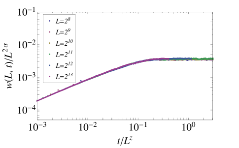
These scaling features are demonstrated by the finite-size scaling of $w(L,t)$ shown in Fig. 1. Perfect data collapse is obtained using the 1D KPZ exponents $\alpha=1/2$ and $z=3/2$. During the growth period the roughness increases nearly linearly on the log-log scale, which indicates power-law growth $w(L,t)\propto t^{2\beta}$. For different system sizes saturation is reached at the same point on the rescaled time axis, confirming the scaling behavior $T_{s}\sim L^{z}$. Finally, the saturation values $w_{s}(L)$ of the roughness function collapse upon rescaling $w(L,t)$ with $L^{2\alpha}$.

A more precise numerical determination of the exponents $\alpha$ and $\beta$, which confirms that their values are given by the ones of the KPZ equation, i.e. $\alpha=1/2$ and $\beta=1/3$, is presented in the appendix. This provides us with strong evidence that the phase field dynamics of a driven-dissipative condensate is indeed described by the KPZ equation, in contrast to the thermal equilibrium case, in which the dynamics of the phase is purely diffusive and thus belongs to the EW universality class Halpin-Healy_KPZ_review . The corresponding dynamical exponent $\beta=1/4$ is different from KPZ universality, however, the value of the static roughness exponent, $\alpha=1/2$, is exactly the same in both cases. This is due to a symmetry of the KPZ equation that is present only in one spatial dimension, and which allows one to show that the static correlations in stationary state are Gaussian Taeuber_book . On the other hand, the dynamical exponent $\beta$ (or equivalently $z$) witnesses quantitatively the difference between KPZ and EW universality.

Before we proceed, let us emphasize an important difference between the phase of a complex field we consider here and the crystal height: the phase is a compact field variable defined on a circle. Without loss of generality the value of $\theta(x,t)$ is in fact bounded to the interval $(-\pi,\pi]$. Consequently, the value of $w(L,t)$ is also bounded from above by $4\pi^{2}$, which inevitably invalidates the static scaling behavior $w_{s}(L)\sim L^{2\alpha}$ if $\alpha$ is positive as expected from the conventional KPZ scenario. However, as long as the field amplitude remains nonvanishing we can let the value of $\psi$ be defined on the Riemann surface, where the value of $\theta$ is in the interval $(-\infty,+\infty)$. With this choice there is no upper bound imposed on $w_{s}(L)$. In numerical simulations, we ensure the requirement $|\psi(x,t)|>0$ by working with low noise. In this regime phase defects do not occur within the spatio-temporal range of our simulations. $\theta(x,t)$ is constructed from $\psi(x,t)$’s complex argument by requiring the phase difference between neighboring space-time points to be less than $\pi$.

III.2 Crossover time scale

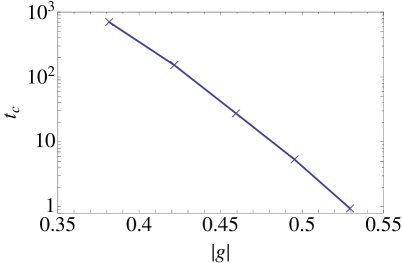
In the above subsection we have established that the phase field dynamics indeed belong to the KPZ universality class. However, it is important to notice that the scaling behavior of $w(L,t)\propto t^{2\beta}$, where $\beta=1/3$ is the KPZ growth exponent, is reached only after a crossover time $t_{c}$. In particular, for weak nonlinearity (i.e. $|g|\ll 1$) the KPZ renormalization group equations lead to a crossover time that scales as $t_{c}\approx t_{0}|g|^{-4}$ Natermann_1d_cross_over_time_scaling , where $t_{0}$ is a microscopic time scale. Scaling behavior of $w(L,t)$ before $t_{c}$ is expected to be governed by the EW growth exponent $\beta=1/4$. In Fig. 2, we investigate the $|g|$ dependence of the crossover time $t_{c}$ at moderate values of $|g|$ (the numerical scheme for the extraction of $t_{c}$ can be found in App. A.2), since extraction of $t_{c}$ in the near equilibrium case, $|g|\ll 1$, is numerically very demanding and $t_{c}$ quickly exceeds the accessible simulation runtimes. We observe that $t_{c}$ increases pronouncedly as $|g|$ decreases (but not yet according to the weak coupling scaling pointed out above). The rapid decrease of $t_{c}$ with increasing non-equilibrium strength is promising for the experimental observation of KPZ scaling behavior, rather than transient EW-like dynamics, before finite size effects set in. We discuss possible experimental settings for observing these phenomena in Sec. V.

Figure 2: (Color online) Dependence of the crossover time $t_{c}$ on the non-equilibrium strength $|g|$. $t_{c}$ decreases pronouncedly as $|g|$ increases. In the numerical results presented here, $|g|$ is tuned by changing $K_{c}=2.4,2.2,2.0.1.8,1.6$ while keeping the other parameters unchanged. Their values are $L=2^{15},r_{c}=-0.1,u_{c}=0.1,\sigma=0.1$.

IV Scaling of the condensate field correlations

In the previous section we have demonstrated numerically that the dynamics of the phase of a one-dimensional polariton condensate follows universal KPZ scaling. In this section we investigate how this scaling manifests in directly observable correlations of the condensate field. Specifically, we consider the correlation functions

$$C_{x}(x_{1},x_{2};t) \equiv \langle\psi^{*}(x_{1},t)\psi(x_{2},t)\rangle,$$ (11)

$$C_{t}(x;t_{1},t_{2}) \equiv \langle\psi^{*}(x,t_{1})\psi(x,t_{2})\rangle,$$ (12)

i.e. the equal time two-point correlation function in space and the temporal autocorrelation function, respectively. These are directly accessible in experiments with exciton-polaritons: Both spatial and temporal coherence can be probed by interference measurements, on the photoluminescence emitted from different regions of the exciton-polariton condensate Polariton_Experiment_1 ; Polariton_Experiment_3 and by combining two images of the condensate taken at different times using, e.g., a Mach-Zehnder interferometer exp_g1_fun_measure , respectively. The visibility of interference fringes yields the correlation functions. Assuming spatial translational invariance of the correlation functions, we calculate the following spatially averaged correlation functions, which are equivalent to the corresponding correlation functions above but in practice help to reduce the statistical error,

$$\begin{split}\bar{C}_{x}(x_{1},x_{2},t)&\equiv\frac{1}{L}\int dy\langle\psi^{*}(x_{1}+y,t)\psi(x_{2}+y,t)\rangle,\\ \bar{C}_{t}(t_{1},t_{2})&\equiv\frac{1}{L}\int dx\langle\psi^{*}(x,t_{1})\psi(x,t_{2})\rangle.\end{split}$$ (13)

IV.1 Spatial correlations

We start with the spatial correlation function $\bar{C}_{x}(x_{1},x_{2},t)$. In Fig. 3 we show the dependence of $\left|\bar{C}_{x}(x_{1},x_{2},t)\right|$ on the distance $|x_{1}-x_{2}|$ at time $t>T_{s}$, from which we clearly identify exponential decay on the semi-logarithmic scale plot. This coincides with the prediction from the effective KPZ description in 1D, and with previous numerical results Wouters_1D_static . However, as anticipated in Sec. III, this static signature would in fact be compatible with thermal equilibrium dynamics of the field $\psi$ and does not unambiguously demonstrate KPZ physics.

Figure 3: (Color online) Behavior of the translation invariant two-point function $\bar{C}_{x}(x_{1},x_{2},t=2.9\times 10^{5}>T_{s})$ at linear system size $L=2^{12}$ on a semi-logarithmic scale. $N_{\mathrm{Traj}}=800$ stochastic trajectories are used to perform the ensemble average. Values of other parameters used here are $r_{c}=-0.1,u_{c}=0.1,\sigma=0.1,K_{c}=3.0$. The exponential decay of $\left|\bar{C}_{x}(x_{1},x_{2},t)\right|$ with respect to $|x_{1}-x_{2}|$ can be clearly identified from this plot.

IV.2 Temporal correlations

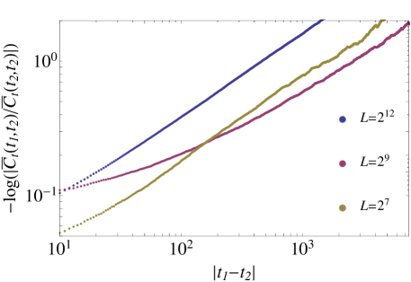
In contrast to the time-independent spatial correlation function discussed in the previous section, the temporal correlation function shows distinct properties depending on whether the system is in thermal equilibrium or not: indeed, based on the effective long-wavelength description of the out-of-equilibrium condensate dynamics in terms of the KPZ equation, we expect stretched-exponential decay of the autocorrelation function, i.e., $\left|\bar{C}_{t}(t_{1},t_{2})\right|=Ae^{-B|t_{1}-t_{2}|{}^{2\beta}}$, with the KPZ growth exponent $\beta=1/3$ and non-universal numbers $A$ and $B$. On the other hand, the purely diffusive EW dynamics of the phase of a condensate in equilibrium entails decay with an exponent $\beta=1/4$. Hence both cases lead to linear growth of $-\log\left(\left|\bar{C}_{t}(t_{1},t_{2})\right|/\left|\bar{C}_{t}(t_{2},t_{2})\right|\right)$ with a slope of $2\beta$ in the double-logarithmic scale used in Fig. 4, which is clearly visible for the upper (at large $|t_{1}-t_{2}|$) curves shown in blue and yellow. Performing linear fits to the data points with $|t_{1}-t_{2}|\in[10^{2},10^{3}]$ we find $\beta=0.311$ and $\beta=0.317$, respectively, in reasonable agreement with the KPZ prediction of $\beta=1/3$ and evidently distinct from the value $\beta=1/4$ for a condensate in equilibrium. For these curves KPZ scaling sets in after a short crossover time difference $t_{c}$, which is due to the relatively large value of the effective non-linear coupling strength $|g|$ in both cases. On the contrary, for the parameters that yield the lowermost (red) curve, the value of $|g|$ is small, and as a result in this case universal scaling behavior is approached only at the largest time differences shown. A fit with $|t_{1}-t_{2}|$ lying in the last half decade of the data shown in the Figure gives $\beta=0.307$, and we expect a value closer to $\beta=1/3$ at time differences larger than those that are accessible within the temporal range of our simulations. The parameters leading to the two lower (red and yellow) curves shown in Fig. 4 are relevant for current experiments with exciton-polaritons as is discussed in the following section.

We note that in a recent work by K. Ji et al. Wouters_1d_temproal , the scaling properties of temporal correlation functions of exciton-polariton condensate were also investigated and among other results, the dynamical exponent $z$ was extracted. For the case of an exciton-polariton condensate without elastic collisions ($\tilde{u}_{c}=0$) and $\tilde{K}_{d}=0$, indicating an infinitely large KPZ nonlinearity $|g|$, they identified KPZ scaling with $z=3/2$ from simulations of a system with dimensionless size $L=2^{7}$ Wouters_1d_temproal . Instead, for the case of an exciton-polariton condensate with elastic collisions, indicating a finite KPZ nonlinearity $|g|$, they reported a dynamical exponent $z\approx 1.7$. This is equivalent to a growth exponent $\beta=\alpha/z=0.5/1.7\simeq 0.294$. As pointed out in Wouters_1d_temproal , this deviation from KPZ scaling could be attributed to finite size effects for the particular parameter choice in this case.

This is compatible with our findings: in fact, in order to unambiguously reveal KPZ scaling in generic cases, relevant to experiments of exciton-polariton condensates, one needs to simulate large enough systems. Here we have simulated systems with sizes up to $L=2^{17}$ and confirm from both the phase correlations (cf. Sec. III and App. A.2) and the condensate field correlations that the growth exponent $\beta$ indeed approaches the expected universal value for generic parameter values. In the following section, based on these findings we study whether this asymptotic behavior can be identified for realistic system parameters.

Figure 4: (Color online) The dependence of $-\log\left(\left|\bar{C}_{t}(t_{1},t_{2})\right|/\left|\bar{C}_{t}(t_{2},t_{2})\right|\right)$ on $|t_{1}-t_{2}|$ for three different sets of parameters in the SCGLE and system sizes. The system size and the parameters for the uppermost (blue) curve are the same as those used in Fig. 3. For the lowermost (at large time differences) curve shown in red, the dimensionless linear system size is $2^{9},$ and the parameters are chosen to match typical values in current experiments with exciton-polaritons (see Sec. V for details). Finally, assuming that a cavity with reduced $Q$ factor is used we obtain the parameters for the middle (yellow) curve, which corresponds to a system size of $2^{7}$. KPZ behavior is revealed by performing linear fits to the data points: with $|t_{1}-t_{2}|\in[10^{2},10^{3}]$ we find $\beta=0.311$ and $\beta=0.317$ for the blue and yellow curves, respectively, while for the red curve a fit with $|t_{1}-t_{2}|$ lying in the last half decade in the above plot, gives rise to $\beta=0.307$. These values should be compared with the KPZ prediction $\beta=1/3$. For all curves $N_{\mathrm{Traj}}=10^{3}$ stochastic trajectories are used.

V Predictions for experimental observation

In the preceding sections we studied the SCGLE as an effective description of the long-wavelength dynamics of a generic driven-dissipative condensate. The microscopic model for the specific case of exciton-polaritons Carusotto2013 differs from the SCGLE in that the diffusion constant is essentially absent and instead of an explicit two-body loss term the pump itself is assumed to be non-linear and saturates at high densities. Slightly above the condensation threshold the saturable pump term can be expanded in the polariton field and we recover the SCGLE, which then reads in dimensionless form

$$\partial_{t}\psi=\left[i\partial_{x}^{2}+(i+u_{d})\left(\frac{p}{u_{d}}-|\psi|^{2}\right)\right]\psi+\zeta.$$ (14)

Here the effective dimensionless two-body loss coefficient $u_{d}$ and the dimensionless pump strength $p$ are given by

$$u_{d}=\frac{\hbar\tilde{\gamma}_{l}R}{2\gamma_{R}\tilde{u}_{c}}(1+2p),\,p=\frac{1}{2}\left(\frac{P}{P_{\mathrm{th}}}-1\right),$$ (15)

with $P$ and $P_{\mathrm{th}}=\tilde{\gamma}_{l}\gamma_{R}/R$ being the pump rate of the excitonic reservoir and its value at threshold, respectively; $R$ is the condensate amplification rate and $\gamma_{R}$ denotes the relaxation rate of the reservoir. Finally, $\tilde{\gamma}_{l}$ is the inverse lifetime of polaritons and $\tilde{u}_{c}$ their interaction strength. Here we measure time and space in units of $\tilde{\gamma}_{l}^{-1}$ and $\sqrt{\hbar/2m_{\mathrm{LP}}\tilde{\gamma}_{l}}$ respectively with $m_{\mathrm{LP}}$ being the effective mass of lower polaritons. The strength of the dimensionless noise field $\zeta$ is $\sigma=\tilde{u}_{c}\sqrt{2m_{\mathrm{LP}}/\hbar^{3}\tilde{\gamma}_{l}}$. Typical values of experimental parameters in 1D exciton-polariton systems are (see, e.g., Ref. 1D_experiment ),

$$\begin{array}[]{l}m_{\mathrm{LP}}=4\times 10^{-5}m_{e},\,\tilde{u}_{c}=5\times 10^{-4}\mathrm{meV}\mu\mathrm{m},\\ \tilde{\gamma}_{l}=0.03\mathrm{ps}^{-1},\,R=3\mu\mathrm{m}\cdot\mathrm{ps}^{-1},\,\gamma_{R}=0.06\mathrm{ps}^{-1},\end{array}$$ (16)

where $m_{e}$ is the mass of the electron.

The lowermost (red) curve in Fig. 4 shows the temporal correlation function $\bar{C}_{t}(t_{1},t_{2})$ in the stationary state for the values given in Eq. (16) and at a dimensionless pump power of $p=0.3$. Due to fact that the corresponding $|g|$ is relatively small, the red curve approaches linear growth characteristic of KPZ scaling only after a large crossover time difference $t_{c}$. As already mentioned in the previous section, a linear fit to the data points with $|t_{1}-t_{2}|$ lying in the last half decade in Fig. 4 yields $\beta=0.307$, indicating that signatures of KPZ physics are nevertheless observable. However, we note that the physical system size corresponding to the dimensionless linear system size of $L=2^{9}$ chosen in this simulation is $\sim 3\times 10^{3}\mu\mathrm{m}$, which is considerably larger than the typical scale $\sim 10^{2}\mu\mathrm{m}$ of current experiments.

Here we propose to make the KPZ physics observable with current experimental system sizes by reducing the cavity $Q$ factor. To this end, we note that KPZ scaling is still observable when, while reducing the physical system size, the dimensionless effective system size can be kept large. A convenient knob to achieve this goal is indeed a reduction of the cavity $Q$ (and thus increase of the decay rate $\tilde{\gamma}_{l}$), which leads to a decrease of the unit of length. (We note that this also facilitates observation of KPZ scaling behavior in equal-time spatial correlations in 2D Altman_2d_driven_SF_2013 .) The middle (yellow) curve in Fig. 4 shows $\bar{C}_{t}(t_{1},t_{2})$ for $\tilde{\gamma}_{l}=1\mathrm{ps}^{-1}$ and a dimensionless linear system size of $L=2^{7}$, corresponding in physical units to $\sim 1.5\times 10^{2}\mu\mathrm{m}$. This means the $Q$ factor is reduced by a factor of $\thicksim 30$ compared to the ones of typical high $Q$ cavities. We note that a decreased $Q$ factor (also indicating an increased noise strength) can destroy the condensate if it is smaller than a threshold value. This is because the reduced cavity lifetime is accompanied by an increased noise level (cf. Eq. (1) and the subsequent discussion), which acts to destroy the condensate. However, we remark here that in the simulation results for this decreased $Q$ factor presented in the following, the system is still condensed, i.e. we are still working in a low noise level regime. In addition to the increase of $\tilde{\gamma}_{l}$, for this simulation we chose a larger value of 6 for the dimensionless prefactor in $u_{d}$ in Eq. (15) instead of $\sim 1$ which we obtain for the parameters given in Eq. (16). This choice magnifies the effective KPZ non-linearity and corresponds to a moderate variation of the experimental parameters only. In fact, the latter are often determined only indirectly via fitting simulations to experimental measurements, and are thus not known with very high precision. In this setting, the exponent of $\beta=0.317$ obtained from the middle (yellow) curve in Fig. 4 indicates that it is promising to search for signatures of KPZ physics in the first-order temporal coherence of 1D exciton-polariton systems when the lifetime of polaritons is rather short, so that the intrinsic non-equilibrium nature is strongly pronounced.

VI Conclusions and Outlook

We investigated scaling properties of the long-wavelength dynamics of 1D driven-dissipative condensate via direct numerical simulations of the SCGLE, and numerically established the connection to 1D KPZ universality. We further numerically confirmed the experimental observability of the non-equilibrium scaling properties of the first order temporal coherence within the typical current experimental setups of exciton-polariton condensates if cavities with a reduced $Q$ factor are used. Similar investigations will be extended to higher dimensions in the future. Moreover, it is intriguing to investigate the dynamics of the driven-dissipative condensates at higher noise level, where in particular phase defects, e.g. phase slips in 1D or vortices in 2D, are expected to play a role in determining the long-wave length scaling properties of the system’s dynamics.

Appendix A Extraction of $\alpha,\beta,$ and $t_{c}$

In this appendix we present a more precise determination of the static roughness exponent $\alpha$ and the dynamical growth exponent $\beta$, and describe how the crossover time scale $t_{c}$ is extracted in numerical simulations.

A.1 Static roughness exponent $\alpha$

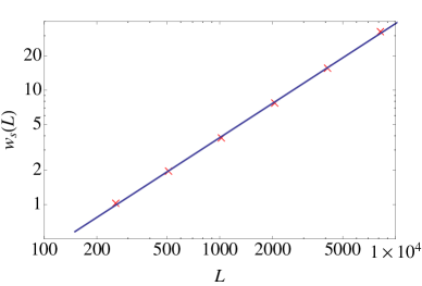
We extract $\alpha$ from the finite-size scaling of $w_{s}(L)$. For given system size $L$, we monitor the value of $w(L,t)$ during a simulation and wait until it reaches a stable value up to statistical fluctuations at the saturation time $T_{s}$. After $T_{s}$, we continue simulating the dynamics to the final time point $T_{f}$ with $T_{f}-T_{s}$ at least two times larger than $T_{s}$. Afterwards $w_{s}(L)$ is extracted according to $w_{s}(L)=(T_{f}-T_{s})^{-1}\int_{T_{s}}^{T_{f}}dt\,w(L,t)$. In Fig. 5 we show the finite size scaling of $w_{s}(L)$ from the direct simulations of the SCGLE. The extracted roughness exponent is $\alpha=0.499$, which is in good agreement with the roughness exponent $\alpha_{\mathrm{KPZ}}$ of the KPZ dynamics being $\alpha_{\mathrm{KPZ}}=1/2$ in 1D Halpin-Healy_KPZ_review .

Figure 5: (Color online) Finite size scaling of $w_{s}(L)$. Points marked by “$\times$” denote the numerical value of $w_{s}(L)$ for system sizes $L=2^{8},2^{9},2^{10},2^{11},2^{12},2^{13}$. The blue line is a linear fit to the data on the log-log scale, from which we extract the roughness exponent $\alpha=0.499$. This is in good agreement with the roughness exponent $\alpha_{\mathrm{KPZ}}$ of the KPZ dynamics in 1D, $\alpha_{\mathrm{KPZ}}=1/2$. Values of parameters used in the simulations are $r_{c}=-0.1,u_{c}=0.1,\sigma=0.1,K_{c}=3.0$.

A.2 Dynamical growth exponent $\beta$ and crossover time scale $t_{c}$

We extract $\beta$ from the time dependent roughness function $w(L,t)$. As pointed before, this exponent is related to the dynamical exponent $z$ and the roughness exponent $\alpha$ via the relation $\beta=\alpha/z$. Its value is expected to be $1/3$ and $1/4$ for effective KPZ and EW dynamics, respectively Halpin-Healy_KPZ_review .

In order to reliably extract the exponent $\beta$ it is important to note that $w(L,t)\propto t^{2\beta}$ is reached only after the initial crossover time scale $t_{c}$ discussed in Sec. III.2. In practice we fit $w(L,t)$ to a power law over a long time window $t\in[t_{e},t_{e}+T]$. We identify the asymptotic scaling by observing how the exponent depends on the lower cutoff time $t_{e}$. As shown in Fig. 6, the fitted exponent $\beta$ first grows with $t_{e}$ but then rapidly reaches a plateau. The value at this plateau represents the asymptotic scaling behavior. We note however that for this scheme to reflect the KPZ scaling, the upper cutoff time $t_{e}+T$ should not reach the finite size saturation time $T_{s}\sim L^{z}$ of the roughness function. If it does, then we expect the extracted exponent $\beta$ to start decreasing again. Thus we extract $\beta$ from the maximum value of the fitted exponent $\beta(t_{e})$. This gives the estimate $\beta=0.335$ consistent with KPZ dynamics, for which $\beta=1/3$ .

Figure 6: (Color online) Upper panel: Time dependence of $w(L,t)$ for different system sizes $L=2^{16},2^{17}$ with $r_{c}=-0.1,u_{c}=0.1,\sigma=0.1,K_{c}=3.0$, on logarithmic scales. Lower panel: $t_{e}$ dependence of extracted $\beta$ at different system sizes $L=2^{16},2^{17}$. The growth exponent of EW dynamics $\beta_{\mathrm{EW}}$ and KPZ dynamics $\beta_{\mathrm{KPZ}}$ are indicated by two lines in the plot to facilitate direct comparison. From the results at system size $L=2^{17}$, we obtain the dynamical exponent $\beta=0.335$ from the maximum value of $\beta(t_{e})$, which is in good agreement with $\beta_{\mathrm{KPZ}}=1/3$.

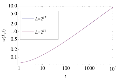
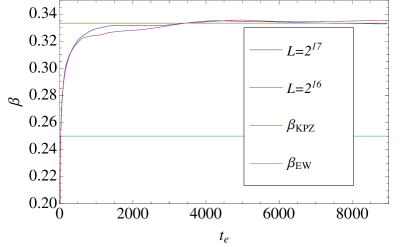
To extract the crossover time $t_{c}$ from the simulations we use the following scheme. At given system size $L$, we fit the time dependent roughness function $w(L,t)$ to a double scaling function $c_{\mathrm{EW}}t^{1/2}+c_{\mathrm{KPZ}}t^{2/3}$ in a time interval that extends from zero until a final time $t_{f}$ well before the finite system size effects set in, i.e. $t_{f}\ll T_{s}$. We then identify $t_{c}$ as the time point where the two scaling functions have the same contribution to the roughness function, i.e. $c_{\mathrm{EW}}t_{c}^{1/2}=c_{\mathrm{KPZ}}t_{c}^{2/3}$, giving rise to $t_{c}=(c_{\mathrm{EW}}/c_{\mathrm{KPZ}})^{6}$.

References

- (1) M. Kardar, G. Parisi, and Y.-C. Zhang, Phys. Rev. Lett. 56, 889 (1986).
- (2) P. C. Hohenberg and B. I. Halperin, Rev. Mod. Phys. 49, 435 (1977).
- (3) J. Kasprzak, M. Richard, S. Kundermann, A. Baas, P. Jeambrun, J. M. J. Keeling, F. M. Marchetti, M. H. Szymańska, R. Andre, J. L. Staehli, V. Savona, P. B. Littlewood, B. Deveaud, and L. S. Dang, Nature 443, 409 (2006).
- (4) K. G. Lagoudakis, M. Wouters, M. Richard, A. Baas, I. Carusotto, R. Andre, Le Si Dang, and B. Deveaud-Pledran, Nature Physics 4, 706 (2008).
- (5) G. Roumpos, M. Lohse, W. H. Nitsche, J. Keeling, M. H. Szymanska, P. B. Littlewood, A. Löffler, S. Höfling, L. Worschech, A. Forchel, and Y. Yamamoto, PNAS 109, 6467 (2012).
- (6) E. Altman, L. M. Sieberer, L. Chen, S. Diehl, and J. Toner, Phys. Rev. X 5, 011017 (2015).
- (7) G. Grinstein, D. Mukamel, R. Seidin, and C. H. Bennett, Phys. Rev. Lett. 70, 3607 (1993).
- (8) V. N. Gladilin, K. Ji, and M. Wouters, Phys. Rev. A 90, 023615 (2014).
- (9) K. Ji, V. N. Gladilin, and M. Wouters, Phys. Rev. B 91, 045301 (2015).
- (10) I. Carusotto and C. Ciuti, Rev. Mod. Phys. 85, 299 (2013).
- (11) L. M. Sieberer, S. D. Huber, E. Altman, and S. Diehl, Phys. Rev. Lett. 110, 195301 (2013); L. M. Sieberer, S. D. Huber, E. Altman, and S. Diehl, Phys. Rev. B 89, 134310 (2014).
- (12) S. F. Edwards and D. R. Wilkinson, Proc. R. Soc. London, Ser. A 381, 17 (1982).
- (13) T. B. Benjamin and J. E. Feir, J. Fluid. Mech. 27, 417 (1967).
- (14) G. Grinstein, C. Jayaprakash and P. Pandit, Physica D 90, 96 (1996).
- (15) M. C. Cross and P. C. Hohenberg, Rev. Mod. Phys. 65, 851 (1993).
- (16) I. Aranson and L. Kramer, Rev. Mod. Phys. 74, 99 (2002).
- (17) S. Mathey, T. Gasenzer, and J. M. Pawlowski, arXiv:1405.7652.
- (18) H. T. C. Stoof, J. Low. Temp. Phys. 114, 11 (1999).
- (19) P. B. Blakie, A. S. Bradley, M. J. Davisb, R. J. Ballagha, and C. W. Gardiner Adv. Phys. 57, 363 (2008).
- (20) M. J. Werner and P. D. Drummond, J. Comp. Phys. 132, 312 (1997).
- (21) E. Marinari, A. Pagnani and G. Parisi, J. Phys. A: Math. Gen. 33, 8181 (2000).
- (22) T. Halpin-Healy and Y. C. Zhang, Phys. Rep. 254, 215 (1995).
- (23) U. Täuber, Critical Dynamics, Cambridge University Press (2014).
- (24) T. Nattermann and L.-H. Tang, Phys. Rev. A 45, 7156 (1992).
- (25) A. P. D. Love, D. N. Krizhanovskii, D. M. Whittaker, R. Bouchekioua, D. Sanvitto, S. A. Rizeiqi, R. Bradley, M. S. Skolnick, P. R. Eastham, R. André, and L. S. Dang, Phys. Rev. Lett. 101, 067404 (2008).
- (26) E. Wertz, A. Amo, D. D. Solnyshkov, L. Ferrier, T. C. H. Liew, D. Sanvitto, P. Senellart, I. Sagnes, A. Lemaître, A. V. Kavokin, G. Malpuech, and J. Bloch, Phy. Rev. Lett. 109, 216404 (2012).