Atmospheric heat redistribution and collapse on tidally locked rocky planets

Abstract

Atmospheric collapse is likely to be of fundamental importance to tidally locked rocky exoplanets but remains understudied. Here, general results on the heat transport and stability of tidally locked terrestrial-type atmospheres are reported. First, the problem is modeled with an idealized 3D general circulation model (GCM) with gray gas radiative transfer. It is shown that over a wide range of parameters the atmospheric boundary layer, rather than the large-scale circulation, is the key to understanding the planetary energy balance. Through a scaling analysis of the interhemispheric energy transfer, theoretical expressions for the day-night temperature difference and surface wind speed are created that reproduce the GCM results without tuning. Next, the GCM is used with correlated-$k$ radiative transfer to study heat transport for two real gases (CO2 and CO). For CO2, empirical formulae for the collapse pressure as a function of planetary mass and stellar flux are produced, and critical pressures for atmospheric collapse at Earth’s stellar flux are obtained that are around five times higher (0.14 bar) than previous gray gas estimates. These results provide constraints on atmospheric stability that will aid in future interpretation of observations and exoplanet habitability modeling.

1 Introduction

M-class (red dwarf) stars comprise around 75% of the total stellar population of the galaxy (Reid et al.,, 2000), and are attractive targets in searches for nearby terrestrial planets because of the well-known scaling of transit probability and radial velocity signal with stellar mass and planetary orbit (Seager et al.,, 2010). Ongoing radial velocity and transit surveys have revealed a number of low mass exoplanets and planet candidates in the stellar neighborhood over the last decade (Mayor et al.,, 2009; Charbonneau et al.,, 2009; Pepe et al.,, 2011; Tuomi et al.,, 2012), and future dedicated missions such as TESS and Plato are likely to discover many more. Furthermore, transit spectroscopy studies of low mass ‘super-Earth’ and ‘mini-Neptune’ planets around M-stars have advanced significantly over the past few years (Bean et al.,, 2010; Croll et al.,, 2011; Demory et al.,, 2012; Kreidberg et al.,, 2013; Fraine et al.,, 2014). Hot, close-in planets around M-stars are likely to be the first rocky planets for which transit spectroscopy and phase curve observations are possible, making them particularly important targets for theoretical study (Selsis et al.,, 2011; Castan and Menou,, 2011; Miguel et al.,, 2011; Samuel et al.,, 2014).

Because of these favorable observational conditions, M-stars are also prime targets in the search for habitable Earth-like planets outside the Solar System. However, if habitable planets around M-stars do exist, they are likely to be very different from Earth. First, M-stars have increased extreme ultra-violet (XUV) emission and coronal mass ejection (CME) for a much longer period than G-class (Sun-like) stars (Khodachenko et al.,, 2007; Lammer et al.,, 2007; Linsky et al.,, 2013). This means that planets around them may suffer greatly enhanced atmospheric loss, particularly if they lack a magnetic field in the early stages of their evolution (Lammer et al.,, 2007; Tian,, 2009; Cohen et al.,, 2014). Because the most volatile gases (H2, N2, Ar etc.) will generally degas into a planet’s atmosphere rapidly during accretion, they are particularly vulnerable to early loss to space. As a result, wide variations in the initial compositions and total masses of the atmospheres of rocky planets around M-stars should be expected.

The low relative luminosities of M-stars mean that planets orbiting close enough to receive Earth-like fluxes are likely to be in tidally resonant or entirely locked states. This means that in some cases, the atmospheres retained by tidally rocky planets after the initial stage of loss to space will be unstable to collapse on the surface (Kasting et al.,, 1993). Despite the fundamental importance of this process, it has to date received relatively little theoretical attention. Previous work has addressed the problem using 3D general circulation models (GCMs) in the context of essentially Earth-like planets (Joshi et al.,, 1997; Joshi,, 2003) and higher mass super-Earths (Wordsworth et al.,, 2011; Selsis et al.,, 2011). Based on these studies, it was found that the stability of a CO2 atmosphere is a strong function of a) the total atmospheric mass, b) the stellar flux received by the planet and c) the radiative transfer model used. Using a GCM with simple gray gas radiative transfer and an Earth-like stellar flux $F_{E}=1366$ W m^-2, Joshi et al., (1997) found that atmospheres above around 0.03 bar $p_{\ce{CO2}}$ were stable. In contrast, Wordsworth et al., (2011) used a GCM with realistic correlated-$k$ radiative transfer, and found that for a 2.3$r_{E}$ planet receiving around 30% of Earth’s incident stellar flux, atmospheric collapse could occur for $p_{\ce{CO2}}$ values as large as $10$ bar.

A comprehensive study of parameter space for the general collapse problem has not yet been performed. Castan and Menou, (2011) modeled the vapor-equilibrium atmospheres of extremely hot super-Earths using an approach first developed to study Io (Ingersoll et al.,, 1985), but did not investigate the transition to uncondensed atmospheres. Heng and Kopparla, (2012) used an analytical approach to construct stability diagrams across a range of parameters. However, they did not investigate the role of real gas radiative transfer or the planetary boundary layer. As will be shown here, both of these processes are critical to understanding atmospheric collapse.

Numerous studies of atmospheric circulation on tidally locked terrestrial planets have also recently been conducted [e.g., Joshi, (2003); Merlis and Schneider, (2010); Heng and Vogt, (2011); Pierrehumbert, 2011b ; Edson et al., (2012); Leconte et al., (2013); Yang et al., (2013)]. These studies have elucidated several dynamical and climatic processes that are likely to be important in the tidally locked regime. However, most of them focused on atmospheres with 1 bar surface pressure and Earth-like composition. Because of the uncertainties in volatile delivery and atmospheric erosion, there is no justification in assuming that Earth-mass planets will possess Earth-like atmospheres (or oceans) in general. Hence study of a wider range of scenarios is necessary.

Understanding atmospheric heat redistribution and collapse is particularly important in the context of future spectral observations of rocky planets. This is true both for transiting planets, and potentially for non-transiting cases if phase curve information can be derived (Selsis et al.,, 2011). Given the complexity of modern GCMs, however, improvements in modeling accuracy must be balanced by advances in basic theory if insight from future observations is to be maximized.

Here a general study of atmospheric stability for tidally locked planets around M-stars is conducted. First, idealized gray-gas GCM simulations are used to study the problem of heat redistribution from day to night side. It is shown that in the physically important limit of slowly rotating optically thin atmospheres, the nightside surface temperature can be estimated analytically, without recourse to any parameters derived from the GCM simulations. Next, the GCM is run in multiband correlated-$k$ mode and used to study collapse across a range of stellar fluxes, atmospheric pressures and planetary masses. We focus on pure CO2 compositions but also study one case where CO is the condensing gas. These gases were chosen because they are common products of volcanic outgassing or thermochemistry following bolide impacts but are not easily destroyed via photolysis or lost to space, unlike e.g. H2O or CH4. It is found that the properties of the planetary boundary layer are more important to the day-night temperature difference than details of the large-scale circulation. In addition, it is shown that the radiative properties of the condensing gas are a key determinant of nightside temperature, and hence the collapse pressure.

In Section 2, the method used for the 3D simulations is described. In Section 3 the idealized gray gas simulations are first presented. Next, a simple theoretical model is used to calculate the nightside surface temperatures produced by the GCM from first principles. Finally, correlated-$k$ GCM results are presented and used to construct simple empirical formulae for the onset of atmospheric collapse for CO2 and CO as a function of stellar flux, total atmospheric pressure and planetary mass. In Section 4 the broader implications of the results are discussed and suggestions for future work are given.

2 Method

For the 3D GCM simulations, the LMD Generic Model is used [e.g., Wordsworth et al., (2011, 2013); Leconte et al., (2013)]. The key model parameters used are shown in Table 1. The LMD model solves the primitive equations on the sphere using the finite-difference approach, with a correlated-k approach for the radiative transfer (Goody and Yung,, 1989; Wordsworth et al., 2010a, ). High-resolution line absorption data for input to the correlated-$k$ model was produced using the open-source software kspectrum and the HITRAN line database (Rothman et al.,, 2009, 2010). CO₂ collision-induced absorption was included using the GBB parameterisation (Wordsworth et al., 2010a, ; Gruszka and Borysow,, 1998; Baranov et al.,, 2004), with extrapolation of the data used at temperatures above 400 K. In all cases the surface topography is assumed to be flat. All simulations were performed assuming a single-component ideal gas atmosphere, with atmospheric condensation represented as in Wordsworth et al., (2011). For CO, the vapor-pressure curve was computed using a Clausius-Clayperon ideal gas relation, with parameters derived from Lide, (2000). Surface horizontal heat transport (due to e.g., the presence of an ocean) is also neglected. Both simplifications are chosen to make the problem more tractable, but they also allow a conservative upper limit on the critical collapse pressure. Unlike in Wordsworth et al., (2011), cloud radiative forcing is also neglected. The likely effects of cloud and aerosol radiative forcing are discussed in Section 4. The surface albedo $A$ is taken to be 0.2, a representative value for rocky planets. For the M-star properties, including the stellar spectrum, data for AD Leo (Gliese 388) is used, as in previous studies (Segura et al.,, 2003; Wordsworth et al., 2010b, ). AD Leo is highly active in the XUV and undergoes frequent flaring events (Shkolnik et al.,, 2009), but these properties do not concern us here as we are focused on radiative processes in the lower atmosphere. Rayleigh scattering is included as in Wordsworth et al., 2010a , although its effects are limited around M-stars because of their red-shifted spectra. The planetary orbit is assumed circular and the obliquity is set to zero. In all simulations the model was run until thermal equilibrium was reached. Complete tidal locking is assumed, allowing the rotation rate $\Omega$ to be calculated from orbital distance via Kepler’s third law as

$$\Omega=\frac{2\pi}{1\mbox{ year}}\left(\frac{M}{M_{\odot}}\right)^{1/2}\left(\frac{L}{L_{\odot}}\right)^{-3/4}\left(\frac{F}{F_{E}}\right)^{3/4}$$ (1)

Here $M$, $L$ and $F$, are stellar mass, stellar luminosity and stellar flux incident on the planet, with $M_{\odot}$, $L_{\odot}$ and $F_{E}$ solar and terrestrial values, respectively. Given $L=0.024L_{\odot}$ and $M=0.4M_{\odot}$ (Pettersen and Coleman,, 1981; Reiners et al.,, 2009), (1) can be written as

$$\Omega=9.2\times 10^{-9}F^{3/4}.$$ (2)

Hence even a planet close enough to receive a stellar flux of $2F_{E}$ (2732 W m^-2) around a typical M-dwarf rotates 20 times less rapidly than Earth. This is the key reason why the effects of rotation on atmospheric circulation are far less important for Earth-like planets around M-stars than for Earth.

For the planetary boundary layer (PBL), the Mellor-Yamada parameterization is used (Mellor and Yamada,, 1982), with the modifications proposed by Galperin et al., (1988) included. This scheme is known to perform well under most conditions in the Martian atmosphere (Haberle et al.,, 1993; Forget et al.,, 1999), which has several similarities to the cases studied here. In brief, the Mellor-Yamada / Galperin (MYG) scheme represents turbulent exchange of momentum and heat between the atmosphere and surface using a second-order closure for the Reynolds-averaged equations. Turbulent kinetic energy $q$ is calculated prognostically assuming a balance between production (via either buoyancy-driven convection or shear in the large-scale flow) and dissipation. Vertical exchange coefficients in the atmosphere and bulk exchange coefficients at the surface are then calculated using $q$, the potential temperature gradient $\partial\Theta/\partial z$, the turbulence mixing length $l$ and empirical dimensionless constants derived from experimental data (Mellor and Yamada,, 1982). The turbulence mixing length is calculated from the empirical scaling law of Blackadar, (1962)

$$l=\frac{l_{0}\mathcal{K}z}{\mathcal{K}z+l_{0}}$$ (3)

where $\mathcal{K}=0.4$ is the von Kármán constant and $l_{0}$ is the maximum attainable mixing length in the boundary layer.

Turbulent exchange coefficients are calculated for every grid point at every time step. Then, the vertical atmospheric diffusion of horizontal momentum and potential temperature are calculated as

$$\left.\frac{\partial\mathbf{u}}{\partial t}\right|_{turb}=\frac{\partial}{\partial z}\left(K_{M}\frac{\partial\mathbf{u}}{\partial z}\right)$$ (4)

$$\left.\frac{\partial\Theta}{\partial t}\right|_{turb}=\frac{\partial}{\partial z}\left(K_{H}\frac{\partial\Theta}{\partial z}\right)$$ (5)

given time $t$, vertical height $z$, horizontal velocity vector $\mathbf{u}=(u,v)$, potential temperature $\Theta$ and eddy momentum and heat diffusion coefficients $K_{M}$ and $K_{H}$. Diffusion coefficients are calculated using Monin-Obukhov scaling (Garratt,, 1994) in terms of $q$, $l$ and the gradient Richardson number, which is defined as the ratio of potential to kinetic energy in the mean flow

$$Ri=\frac{g}{\Theta}\frac{\partial\Theta}{\partial z}\left[\left(\frac{\partial u}{\partial z}\right)^{2}+\left(\frac{\partial v}{\partial z}\right)^{2}\right].$$ (6)

In discrete form, a bulk Richardson number can also be defined as

$$Ri_{B}=\frac{g\Delta\Theta/\Theta}{|\mathbf{u}|^{2}/\Delta z},$$ (7)

where $\Delta z$ is the height from the surface and $\Delta\Theta$ is the potential temperature difference between the surface and the atmospheric region under consideration.

At the surface, bulk exchange is calculated as

$$\mathcal{F}(f)=C_{D}\rho_{a}|\mathbf{u}|(f_{a}-f_{s})$$ (8)

where $\mathcal{F}$ is the flux of quantity $f$, $C_{D}$ is the bulk drag coefficient and $\rho_{a}$ and $|\mathbf{u}|$ are the atmospheric density and wind speed in the first atmospheric layer, respectively. $f_{a}$ and $f_{s}$ are the values of $f$ in the first atmospheric layer and at the surface, respectively; for $f=|\mathbf{u}|$, $f_{s}=0$. Finally, the bulk drag coefficient is calculated as

$$C_{D}=\left(\frac{\mathcal{K}}{ln[z/{z_{0}}]}\right)^{2}$$ (9)

where $z_{0}$ is the roughness height. $z_{0}$ is essentially a free parameter in an exoplanet context, although it can be constrained for terrestrial planets based on solar system radar observations [e.g., (Downs et al.,, 1975; Head et al.,, 1985; Rosenburg et al.,, 2011)]. Here we adopt a representative value for rocky surfaces (Table 1). Note that the dependence of $C_{D}$ on $z_{0}$ is weak, so even order of magnitude variations in roughness length have only a limited effect on the boundary layer behavior (Wordsworth et al.,, 2011).

3 Results

3.1 Idealised 3D GCM simulations

To begin the investigation, we examine idealized 3D simulations where gray gas radiative transfer is assumed and the atmospheric extinction of incoming starlight is neglected. Three surface pressures are used: 0.01, 0.1 and 1 bar. The gas is assumed to have the thermodynamic properties of CO2. Earth radius $r_{p}=r_{E}$, gravity $g=g_{E}$ and incoming stellar flux $F=F_{E}=1366$ W m^-2 are assumed. With a hemispheric mean approximation for the two-stream radiative transfer, total optical depth is

$$\tau=\frac{\kappa p_{s}}{g\overline{\cos\alpha}},$$ (10)

with $p_{s}$ surface pressure, $g$ gravity and $\overline{\cos\alpha}=0.5$ the mean cosine of infrared emission angle. We set $\kappa=5.0\times 10^{-5}$ m²/kg, yielding $\tau=0.1$ at 0.1 bar, which places us in an optically thin radiative regime for 2 of the 3 simulations. As will be seen, this is the most relevant limit to study for most (but not all) situations where collapse may occur.

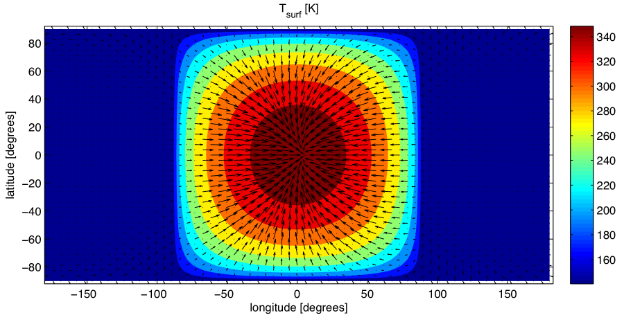
Figure 1 shows the modeled surface temperature and winds for the intermediate $p_{s}=0.1$ bar simulation. The picture is a familiar one: a large thermal gradient on the dayside and almost uniform, low temperature on the nightside, with converging surface winds near the substellar point. To a first approximation the flow is longitudinally symmetric, indicating the limited effect of planetary rotation. This is expected based on a dimensional analysis: the ratio of the equatorial Rossby deformation radius to the planetary radius

$$\frac{L_{Ro}}{r_{p}}=\sqrt{\frac{R}{c_{p}}\frac{\sqrt{c_{p}T_{e}}}{2\Omega r_{p}}}$$ (11)

is 2.06, indicating a dynamical regime where rotation has little effect on the large-scale circulation (Leconte et al.,, 2013). In (11), $R$ and $c_{p}$ are the specific gas constant and specific heat capacity at constant pressure (for CO2 here), $r_{p}$ is planetary radius and $T_{e}=[(1-A)F/4\sigma]^{\frac{1}{4}}$ is the global equilibrium temperature.

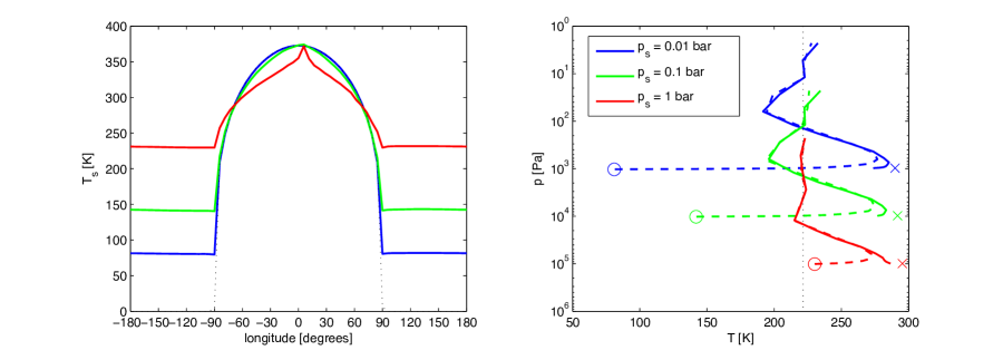
Figure 2 (left) shows the surface temperature at the equator for all simulations as a function of longitude. The dayside temperature is extremely close to the local equilibrium temperature (dotted black line) in the 0.01 and 0.1 bar cases, with some deviations occurring at 1 bar. This indicates that the thermal energy transported to the nightside is generally a small fraction of the total — a fact we will exploit when developing the analytical model in the next section.

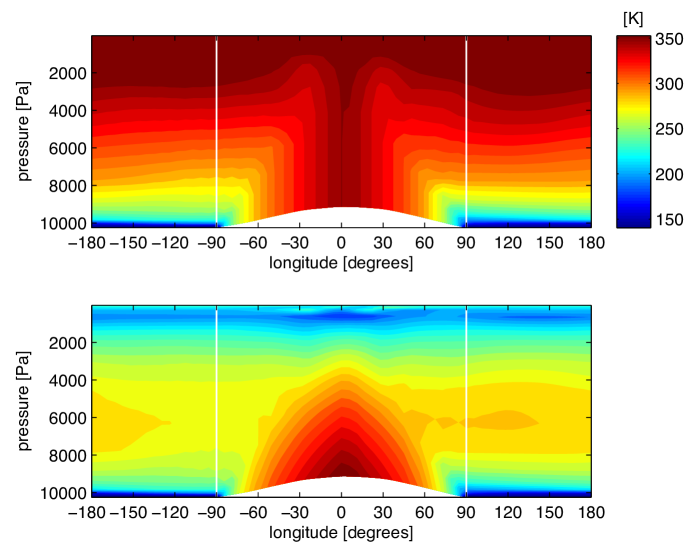
Figure 2 (right) shows the day and nightside averaged vertical temperature profiles in the three simulations. All profiles approach the skin temperature $T_{skin}=2^{1/4}T_{e}$ at low pressures, as is expected given the gray radiative transfer. Remarkably, atmospheric temperatures vary little between day and night hemispheres until extremely close to the surface, despite the large differences in day and night surface temperatures. This general feature of tidally locked terrestrial planet atmospheres, which has been noted previously [e.g., (Merlis and Schneider,, 2010; Pierrehumbert, 2011b, )], indicates that they are in a weak temperature gradient (WTG) regime (Sobel et al.,, 2001). This can also be seen from Figure 3, which shows longitude-pressure plots of mean atmospheric temperature and potential temperature for the $p_{s}=0.1$ bar case. Potential temperature $\Theta$ is related to temperature $T$ as $\Theta=T(p_{s}/p)^{R/c_{p}}$, where $p$ and $p_{s}$ are the atmospheric and surface pressure.

To gain further insight into the planetary energy balance, we next study the surface sensible and radiative heat balance. Figure 4 shows a plot of net sensible heat flux, absorbed stellar radiation, and downwards/upwards infrared radiative fluxes at the surface as a function of longitude for all three simulations. The upwards infrared flux closely matches the absorbed stellar radiation in the 0.01 and 0.1 bar simulations. The downwards infrared radiation is almost constant in all cases, because the atmospheric temperature varies little with longitude. The sensible heat flux is the most interesting: it exhibits a double-peaked structure on the dayside but drops to close to zero on the nightside.

The behavior of the sensible heat flux is a natural consequence of dry boundary layer physics, as captured by the MYG scheme in the model. On the dayside, fluxes are large because the high stellar energy input to the surface creates an intense, permanent convection layer. In this case, the bulk Richardson number $Ri_{B}$ is extremely low and hence the drag coefficients in (5-8) are large, leading to efficient thermal coupling with the surface. The double-peaked structure occurs because of the surface wind pattern, which we explore in more detail shortly.

On the nightside, the strong stratification created by the temperature inversion inhibits boundary layer turbulence. The only source of turbulent kinetic energy is the weak large-scale circulation. Mixing is strongly inhibited and the sensible heat flux declines to very low values. A familiar (although less extreme) analogy to this situation is the polar night on Earth. There, radiative cooling to space dominates the surface heat budget, the planetary boundary layer becomes near-laminar and extremely thin, and the magnitude of the sensible heat flux declines to a low value within days (Cerni and Parish,, 1984).

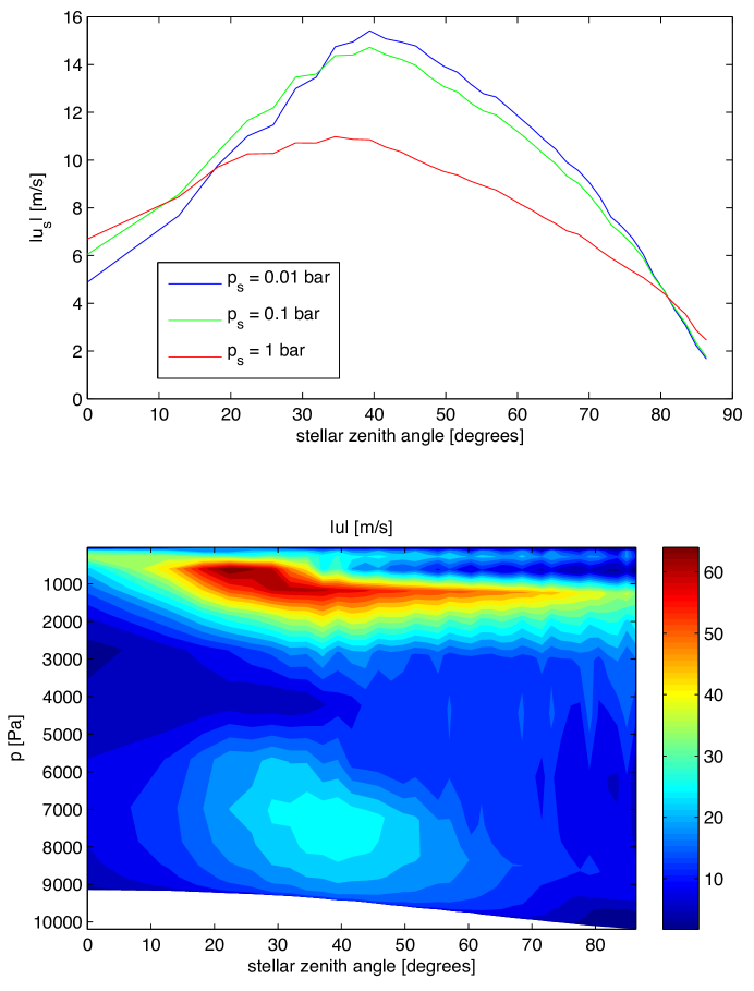
Figure 5 (top) shows the time-averaged surface wind speed $\theta_{z}$ in the model as a function of stellar zenith angle. The data in Figure 5 was derived by binning the 2D surface velocity magnitude fields $|\mathbf{u}|=\sqrt{u^{2}+v^{2}}$ from the GCM into concentric circles around the substellar point and averaging. All simulations show a peak at around $\theta_{z}=40^{\circ}$, with similar profiles at 0.01 and 0.1 bar and a reduced peak wind speed in the 1 bar case. The reduction in wind speed near the substellar point explains the dip in the sensible heat flux there (Fig. 4) and hence the sharp peak in surface temperature in the 1 bar case. For the 0.01 and 0.1 bar cases, the sensible heat flux is too low to significantly reduce the dayside surface temperatures.

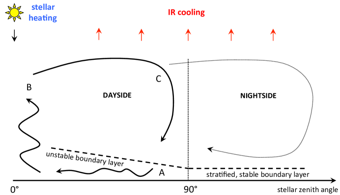
The 0.1 bar plot of $|\mathbf{u}|$ vs. $\theta_{z}$ and $p$ (bottom) shows an intense jet (up to 60 m s^-1) high in the atmosphere. This is the outward branch of the flow seen near the surface in Fig. 1; the wind speed minimum around the $p_{s}/2$ level indicates the transition between flow to/from the substellar point. Essentially, when the planetary rotation rate is low, the large-scale circulation has the form of a single planetary-sized convection cell (see Fig. 6 for a schematic). In the next section, it is shown that the surface wind speed can be explained by a scaling analysis.

It is interesting to compare the 1 bar, $\tau=1$ results in Fig. 2 (left) with those from the Joshi et al., (1997) study of atmospheric collapse. There, lower day/night side differences were found, with nightside temperatures of around 260-270 K, compared to around 240 K in this study. This suggests that heat redistribution by the atmosphere was much more efficient in their model. The Joshi et al., (1997) model used a simple boundary layer representation based on a quadratic formulation (Joshi et al.,, 1995), which may have over-represented the efficiency of coupling between the atmosphere and the surface. The subtle issue of accurate sensible heat flux parameterization in the strongly stably stratified regime is discussed further in Section 4.

3.2 Analytical model

Despite the complexity of the GCM used, the results described in the last section appear essentially simple. To gain a deeper understanding, we now reproduce them using a purely analytical approach. Our goal in this section is to calculate the nightside surface temperature $T_{n}$ from first principles, without using any GCM-derived coefficients.

To aid development of the model, a schematic of the key features of the circulation is given in Figure 6. Inspired by Figure 3, we will assume that the atmosphere can be treated as horizontally isothermal outside of the dayside convective zone. Given this, a three-box model of energy exchange between the dayside surface, atmosphere and nightside surface can then be constructed. Our approach is somewhat similar to that of Pierrehumbert, 2011b and Yang and Abbot, (2014), except here we are after analytical results and hence avoid ad-hoc tuning to the GCM simulations.

Given a dry, single-component atmosphere that is transparent in the visible and gray in the infrared and surface of emissivity equal to 1, the local surface energy balance may be written

$$\sigma T_{s}^{4}=(1-A)S(\psi,\lambda)+GLR+C_{D}c_{p}\rho_{a}|\mathbf{u}|(T_{a}-T_{s}).$$ (12)

Here $S(\psi,\lambda)=F\cos\theta_{z}$ is the local stellar flux, $\psi$, $\lambda$ and $\theta_{z}$ are longitude, latitude and stellar zenith angle, respectively, $GLR$ is the downwards infrared radiative flux and $T_{a}$ is the near-surface atmospheric temperature. Similarly, in the absence of visible absorption the vertically integrated local atmospheric energy balance may be written

$$OAR+GLR=\mathcal{A}\sigma T_{s}^{4}+\mathcal{D}+C_{D}c_{p}\rho_{a}|\mathbf{u}|(T_{s}-T_{a})$$ (13)

where $OAR$ is the outgoing infrared radiation emitted to space by the atmosphere and $\mathcal{A}$ is the frequency-averaged atmospheric absorptance in the infrared. $\mathcal{D}$ represents the effects of dynamical transport and will disappear once we assume the atmosphere to be isothermal and perform horizontal averaging. The third term on the right hand side of (13) is the sensible heat flux: it is simply (8) with $f=c_{p}T$ the quantity undergoing exchange.

Next, we define

$$B_{d}=\frac{\int_{d}\sigma T_{s}^{4}dA}{2\pi r_{p}^{2}}$$ (14)

$$B_{n}=\frac{\int_{n}\sigma T_{s}^{4}dA}{2\pi r_{p}^{2}}$$ (15)

with $\int_{d}dA$ and $\int_{n}dA$ surface integrals over the planet’s day and nightsides, respectively. Applying these integrals separately to (12) in turn and averaging (13) over the entire planet, we obtain

$$B_{d} = \frac{1}{2}(1-A)F+GLR+C_{D}c_{p}\rho_{a}\overline{|\mathbf{u}|(T_{a}-T_{d})}$$ (16)

$$B_{n} = GLR+C_{D}c_{p}\rho_{a}\overline{|\mathbf{u}|(T_{a}-T_{n})}$$ (17)

and

$$OAR+GLR=\frac{1}{2}\mathcal{A}B_{d}+\frac{1}{2}\mathcal{A}B_{n}+\frac{1}{2}C_{D}c_{p}\rho_{a}\overline{|\mathbf{u}|(T_{d}-T_{a})}+\frac{1}{2}C_{D}c_{p}\rho_{a}\overline{|\mathbf{u}|(T_{n}-T_{a})}$$ (18)

where $T_{d}$ and $T_{n}$ are the mean dayside and nightside surface temperatures, respectively. Note that because of the isothermal assumption, most global average and local atmospheric values are the same [e.g., $\overline{OAR}=(4\pi r_{p}^{2})^{-1}\int_{\Sigma}OARdA=OAR$]. We allow for the possibility of horizontal variations in $|\mathbf{u}|$ and $T_{d}$, however, by retaining the overbar for the sensible heat terms.

If the atmosphere can be assumed to be optically thin, $\mathcal{A}\approx\tau$ and $OAR\approx GLR\approx\tau B_{a}$ (Pierrehumbert, 2011a, ). Then (16-18) can be simplified to

$$B_{d} = \frac{1}{2}(1-A)F+\tau B_{a}+C_{D}c_{p}\rho_{a}\overline{|\mathbf{u}|(T_{a}-T_{d})}$$ (19)

$$B_{n} = \tau B_{a}+C_{D}c_{p}\rho_{a}\overline{|\mathbf{u}|(T_{a}-T_{n})}$$ (20)

$$4B_{a} = B_{d}+B_{n}+C_{D}c_{p}\rho_{a}\overline{|\mathbf{u}|\left[(T_{d}-T_{a})+(T_{n}-T_{a})\right]}/\tau$$ (21)

3.3 Purely radiative case

First we examine the artificial but instructive limit where $C_{D}\to 0$ and the only permitted surface-atmosphere energy exchange is radiative. Remaining in the optically thin regime, (19-21) reduce to

$$B_{d} = \frac{1}{2}(1-A)F+\tau B_{a}$$ (22)

$$B_{n} = \tau B_{a}$$ (23)

$$4B_{a} = B_{d}+B_{n}$$ (24)

Hence

$$B_{n}=\frac{\tau}{2-\tau}\frac{(1-A)F}{4}.$$ (25)

Because we have already assumed $\tau<1$, this may be further approximated as

$$B_{n}\approx\frac{\tau(1-A)F}{8}.$$ (26)

Hence using the definition of optical depth (10) with $\overline{\cos\alpha}=0.5$,

$$T_{n}\approx\left(\frac{(1-A)F\kappa p_{s}}{4\sigma g}\right)^{1/4}.$$ (27)

In the thin, isothermal limit with zero sensible heat fluxes, this solves the problem of the surface nightside temperature for a given atmospheric opacity and stellar flux. Note that (27) can also be derived by neglecting a) the radiative back-reaction of the atmosphere on the dayside surface and b) the back-reaction of the nightside surface on the atmosphere. In other words, it relies on the assumption that the dayside temperature is unaffected by the presence of an atmosphere, and the atmospheric temperature is unaffected by the heat received from the nightside.

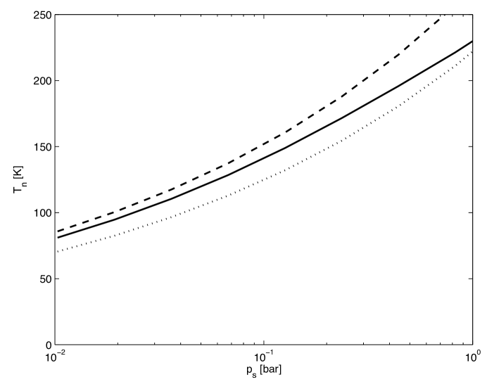
Sticking in the numbers to (27) for the three ideal GCM cases presented in Section 3.1, we get $T_{n}=$ 70.4, 125.2 and 222.7 K for $p=$ 0.01, 0.1 and 1 bar, respectively. These values are reasonably close to those calculated by the GCM [see Fig. 2 (left)], which is impressive given the simplicity of the derivation. However, there is a systematic bias towards lower temperatures, which is expected given that we are neglecting all turbulent surface-atmosphere heat exchange. We henceforth refer to (27), which provides a lower limit to $T_{n}$ for optically thin atmospheres, as the thin radiator temperature.

3.4 Inclusion of the dayside sensible heat flux

Now we relax the assumption of zero sensible heat fluxes. It might be tempting to include all terms and attempt to solve (19-21) numerically. However, a little more physical insight will allow these equations to be simplified further. Specifically, we invoke the fact that radiative fluxes dominate sensible fluxes in the strongly stratified nightside boundary layer (see Fig. 4) and drop terms involving $(T_{a}-T_{n})$ in (20) and (21). We also assume $B_{n}<<B_{a}$ and $\tau B_{a}<<\frac{1}{2}(1-A)F$. Hence (19-21) become

$$B_{d} \approx \frac{1}{2}(1-A)F$$ (28)

$$B_{n} \approx \tau B_{a}$$ (29)

$$4B_{a} \approx B_{d}+C_{D}gc_{p}\overline{|\mathbf{u}|(T_{d}/T_{a}-1)}/(2\kappa R).$$ (30)

where the ideal gas law and (10) have been used. We rewrite $\overline{|\mathbf{u}|(T_{d}/T_{a}-1)}$ as $\chi{|\mathbf{u}|(T_{d}/T_{a}-1)}$, where $|\mathbf{u}|$, $T_{d}$ and $T_{a}$ are now taken to be hemispheric mean values and $\chi$ is a factor that accounts for the fact that temperature peaks at $\theta_{z}=0$, whereas $|\mathbf{u}|$ peaks around $40^{\circ}$. To this level of approximation we may write $T_{d}/T_{a}\propto\cos\theta_{z}$ and $|\mathbf{u}|\propto\sin\theta_{z}$, yielding $\chi=\int_{0}^{\pi/2}\cos^{2}\theta_{z}\sin\theta_{z}d\theta_{z}=1/3$. By defining a dimensionless atmospheric temperature $\tilde{T}=T_{a}/T_{d}$ and velocity $\tilde{U}=|\mathbf{u}|/U_{0}$, with

$$U_{0}=(1-A)F\frac{\kappa}{\chi C_{D}g}\frac{R}{c_{p}}$$ (31)

we can rewrite (30) as

$$4\tilde{T}^{4}-1=\tilde{U}(\tilde{T}^{-1}-1).$$ (32)

(32) defines $T_{a}$ (and hence $T_{n}$) as a function of $T_{d}$ if $|\mathbf{u}|$ is known.

3.5 An equation for $|\mathbf{u}|$

To close equation (32), we next utilize the WTG approximation. WTG scaling for velocity has been analyzed in a shallow water context for Earth (Sobel et al.,, 2001) and was recently applied to hot Jupiters (Perez-Becker and Showman,, 2013), suggesting that it should also be useful here. Nonetheless, the central role of the planetary boundary layer in interhemispheric heat transport on rocky planets means that the approach we take here is rather different from what has been done previously.

The thermodynamic equation (Vallis,, 2006)

$$\frac{DI}{Dt}+\frac{p}{\rho}\nabla\cdot\mathbf{u}=\mathcal{H}$$ (33)

with $I$ internal energy, $p$ pressure, $\rho$ density, $\mathbf{u}$ velocity, $D/Dt$ the advective derivative and $\mathcal{H}$ the diabatic heating rate in W/kg may be simplified in the WTG, ideal gas limit to

$$\nabla\cdot\mathbf{u}=\frac{1}{RT_{a}}\mathcal{H}.$$ (34)

The essence of (34) is that in the absence of time-varying or advective effects, expansion of a fluid column in the bulk atmosphere due to heating must be compensated by outward flow of material to eliminate the horizontal thermal gradient. $\mathcal{H}$ represents the net effect of all heating and cooling processes in a given region. We first focus on the local radiative heating of the atmosphere by the ground $\mathcal{H}_{rad,s}$ and determine the probable scaling. Momentarily replacing the unknown $T_{a}$ by $T_{d}$, we can write

$$\frac{U_{1}}{L}\sim\frac{1}{RT_{d}}\mathcal{H}_{rad,s}$$ (35)

and hence

$$U_{1}\sim\frac{L\kappa(1-A)F}{2RT_{d}}.$$ (36)

$L$ is a characteristic horizontal length scale that we take here to be the planetary radius $r_{p}$. The new velocity scale $U_{1}$ may be related to $U_{0}$ by defining the dayside scale height $H_{d}=RT_{d}/g$, resulting in

$$U_{1} \sim \frac{r_{p}}{H_{d}}\frac{(1-A)F\kappa}{2g}$$ (37)

$$U_{1} \sim \tilde{L}U_{0}$$ (38)

with the dimensionless length

$$\tilde{L}=\frac{\chi C_{D}r_{p}}{2H_{d}}\frac{c_{p}}{R}.$$ (39)

Given a roughness height of $1\times 10^{-2}$ m and height of the first model layer $z\sim 10$ m, $C_{D}=0.0034$. For an Earth-mass planet with CO2 atmosphere, this yields $\tilde{L}=2.4$. We shall see that $\tilde{L}$ gives a measure of the strength of $|\mathbf{u}|$ and hence of the sensible heat flux from the dayside to the atmosphere.

Next we return to (34), write $\nabla\cdot\mathbf{u}\sim|\mathbf{u}|/r_{p}$, and include the dayside radiative cooling and sensible heating terms. This yields

$$\frac{|\mathbf{u}|}{r_{p}}=\frac{1}{RT_{a}}\left(\kappa\sigma T_{d}^{4}-2\kappa\sigma T_{a}^{4}+\frac{g\chi C_{D}|\mathbf{u}|c_{p}(T_{d}-T_{a})}{RT_{a}}\right)$$ (40)

with the final term on the right hand side the sensible heat flux to the atmosphere in W m^-2 divided by a factor $p_{s}/g$ to get the heating rate per unit mass. Using the previously derived scaling relations, (40) can be used to create an expression for the dimensionless velocity

$$\tilde{U}=\frac{\tilde{L}(1-2\tilde{T}^{4})}{\tilde{T}+2\tilde{L}(1-\tilde{T}^{-1})}.$$ (41)

Substituting (41) into (32) we get

$$(4\tilde{T}^{4}-1)\left[\tilde{T}+2\tilde{L}(1-\tilde{T}^{-1})\right]-\tilde{L}(1-2\tilde{T}^{4})(\tilde{T}^{-1}-1)=0.$$ (42)

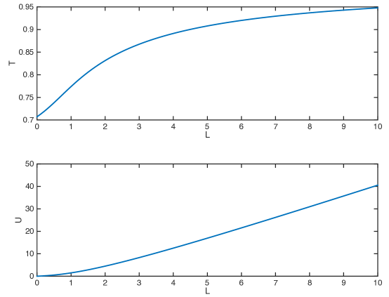
This polynomial in $\tilde{T}$ and $\tilde{L}$ can be solved by Newton’s method, resulting in expressions for $\tilde{T}$ and $\tilde{U}$ as functions of $\tilde{L}$, which is a fixed parameter for a given planet. The result is shown in Fig. 7. Given $\tilde{L}=2.4$, we find $\tilde{U}=6.2$ and $\tilde{T}=0.85$. For $U_{0}=1.2$ m s^-1, $|\mathbf{u}|=7.4$ m s^-1, which is reasonably close to the surface values in Fig. 5.

Fig. 8 shows the nightside surface temperature predicted by (29) given this result vs. gray gas results from the GCM for a range of surface pressures. As can be seen, the correspondence is close over most of the range of pressures studied, with (29) slightly overpredicting the GCM value of $T_{n}$. The ‘thin radiator temperature’ (20) underpredicts the GCM results by a larger margin. The divergence around 1 bar can be explained by the fact that the atmosphere becomes optically thick at that pressure. A similar approach to scaling for the optically thick case should also be possible, and will be addressed in future work.

3.6 Multiband 3D GCM simulations

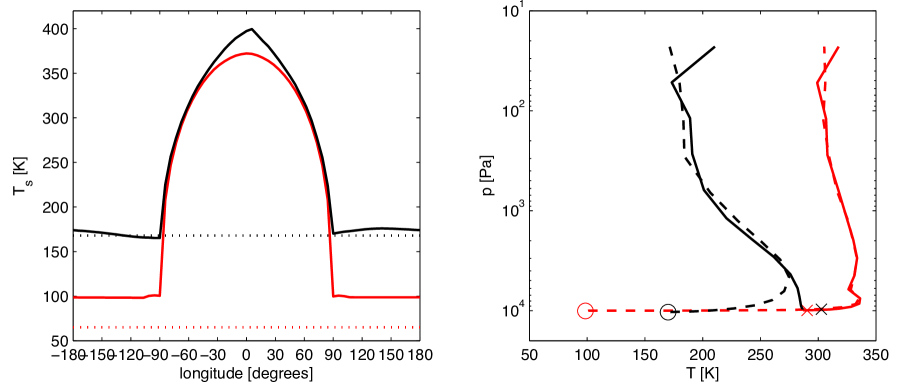
Having developed a comprehensive understanding of the key features of interhemispheric heat transport in the gray gas simulations, we now address the full atmospheric collapse problem in the GCM with correlated-$k$ radiative transfer. Figure 9 shows surface and atmospheric temperatures in 0.1 bar GCM simulations with the same planetary parameters as for Fig. 3 but using correlated-$k$ radiative transfer and assuming CO2 (black lines) and CO (red lines) composition. The dotted lines on the left indicate condensation temperatures at 0.1 bar. As can be seen, the nightside is around 70 K colder for CO than for CO2. Nonetheless, the greater volatility of CO means that it remains stable, whereas in the CO2 simulation the nightside temperature dips below the condensation temperature.

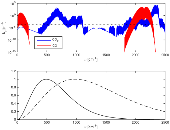
The inefficient heat transport of the CO atmosphere can be understood by comparing the infrared absorption spectra of CO2 and CO (Figure 10). As can be seen, the absorption bands of CO2 are wide and fall near the peak of the Planck function at both temperatures, while those of CO are thinner and far from the Planck function peak, particularly at low temperatures. The ultimate reason for this is molecular structure: CO is diatomic, with a permanent dipole, and so the infrared absorption spectrum consists of a single weak rotation band at low wave numbers and the fundamental vibration-rotation band centered at 2143.27 cm^-1 (Goody and Yung,, 1989). CO2, in contrast, has no rotation band due to the lack of a permanent dipole but intense vibration-rotation bands centered on 667 cm^-1 (15 $\mu$m) and 2325 cm^-1 (4.3 $\mu$m) due to the $\nu_{2}$ and $\nu_{3}$ fundamental modes, with complications due to Fermi resonances, Coriolis interactions and increased occupancy of higher vibrational levels at moderate temperatures. As demonstrated by the analysis in the preceding sections, the nightside temperature depends critically on the atmospheric opacity, and hence weakly absorbing gases cause extremely high surface temperature contrasts. In future observations of hot rocky planets, it should be possible to utilize this effect to constrain atmospheric properties.

The remarkably high atmospheric temperatures in the CO case (Figure 10; right) appear paradoxical, but they can also be explained by the radiative properties of the gas. CO is inefficient enough at radiating energy either to space or the surface that almost the entire atmosphere thermally equilibrates with the part of the surface where sensible heat fluxes peak: the dayside near the substellar point. Clearly, if more radiatively active gases or aerosols were present in a CO-dominated atmosphere even in trace amounts, the behavior of the system could change considerably. Because of the subtlety of this problem, we leave the calculation of collapse pressure for CO and other radiatively inactive, volatile gases such as N2 to future work.

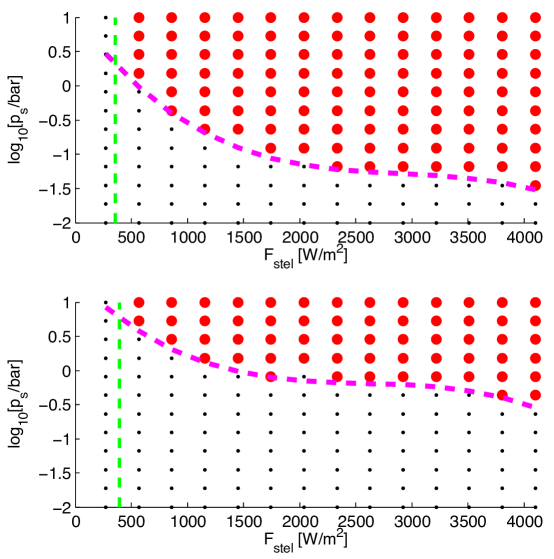
With the atmospheric composition restricted to CO2 only, condensation was included, and GCM simulations were performed on a 14$\times$12 grid in the space of stellar flux and initial atmospheric pressure, for a planet with Earth’s mass and radius. Figure 11 shows the results. The contour values show minimum surface temperature $T_{min}$. In the white regions of the plot, $T_{min}<T_{cond}$, where $T_{cond}$ is the condensation temperature, and the atmosphere has begun to collapse on the surface.

As can be seen, the onset of atmospheric collapse is a strong function of surface pressure, with collapse occurring for any stellar flux given $p_{s}<0.1$ bar. Collapse also occurs at all surface pressures for the lowest stellar flux studied (0.2 $F_{0}$ or $273.2$ W m^-2). These fluxes are below even the values for the exoplanet candidate GJ581d, which we have shown can support stable CO2 atmospheres above pressures of around 10 bar (Wordsworth et al.,, 2011). The approximate Kombayshi-Ingersoll limit for CO2 (Pierrehumbert, 2011b, ) is indicated by the vertical green dashed line.

The prediction of CO2 collapse at around 0.1 bar contrasts with the results of Joshi et al., (1997), who found that CO2 atmospheres with pressures as low as 30 mbar would be stable against collapse. There are two reasons for this discrepancy. First, as discussed earlier, in Joshi et al. predict somewhat higher nightside temperatures than found here even when we use the same gray gas radiative transfer as they did. Second, models with gray gas radiative transfer significantly overestimate coupling between the atmosphere and nightside surface. Particularly at pressures less than 1 bar, windows in the absorption spectrum (e.g., at wavenumbers less than 500 cm^-1 for CO2) allow the surface to emit radiation directly to space, greatly increasing cooling rates.

It is also interesting to compare the results given here with the analytical predictions of Heng and Kopparla, (2012). Essentially the entire range spanned by Fig. 11 is in their predicted ‘stable atmosphere’ region (see their Fig. 3), indicating that their $t_{adv}<t_{rad}$ criterion does not represent a sufficient condition for atmospheric stability independent of atmospheric pressure. Conversely, $t_{adv}>t_{rad}$ does not appear to be sufficient for instability in all cases, because in simulations assuming a 10 M_⊕ planet, stable atmospheric solutions at high CO2 pressures were also found [Fig. 11 (bottom)]. In the highly irradiated regime where the flow Mach number can approach the sound speed, however, their approach may still be applicable. Applying 3D circulation models with real gas radiative transfer to this problem will be an interesting topic for future research.

Finally, using the data shown in Figure 11, empirical formulae of the critical collapse pressure $p_{crit}$ vs. stellar flux were created according to the expression

$$log_{10}\left[\frac{p_{crit}}{1~{}\mbox{Pa}}\right]=c_{1}F_{s}^{3}+c_{2}F_{s}^{2}+c_{3}F_{s}+c_{4}$$ (43)

with the constants $c_{i}$ derived by a least-squares fit. The results are shown in Figure 11, with the coefficients given in Table 2.

The atmosphere collapses at higher pressures in general on higher mass planets for several reasons. First, the increase in gravity means a lower column mass for a given pressure. This means the total atmospheric opacity is also lower, and hence the nightside temperature decreases. In addition, higher planetary radii mean the advection time $t_{adv}=r_{p}/|\mathbf{u}|$ should be smaller if $|\mathbf{u}|$ remains constant. However, in the WTG regime the scaling of $\tilde{U}$ with $\tilde{L}$ and hence $r_{p}$ suggests that this effect should be less important.

The decrease in the critical collapse pressure with stellar flux can be understood by reference to (27). Increasing stellar flux implies a greater amount of heat is transported to the nightside, and hence a lower total pressure can be achieved before collapse occurs. Because at fixed stellar luminosity we increase stellar flux by moving the planet inwards, the effects of rotation on the circulation must eventually become important. However, its importance appears to be secondary for the range of cases studied here.

4 Discussion

Atmospheric collapse is likely to be of fundamental importance for tidally locked rocky planets. The analysis in the preceding section has demonstrated that despite the fact that the collapse problem involves coupling between several complex processes (radiative transfer, the large-scale circulation and boundary layer turbulence), its key features can be understood using an entirely analytical approach.

How robust are these results? Clearly, modifying effects such as ocean heat transport or intense tidal heating of the planetary interior could result in more stable atmospheres than found here. The presence of radiatively active trace gases would also render an atmosphere more stable than the single-component cases studied here, by increasing the radiative coupling between the atmosphere and night side of the planet. A similar role could be played by aerosols released by volcanism or by surface lifting of dust. Clouds can also potentially contribute to greenhouse warming on the nightside, as we found previously for CO2 in Wordsworth et al., (2011), although thermodynamics disfavours nightside H2O cloud formation for Earth-like tidally locked planets (Yang et al.,, 2013). Further modeling will be required to assess the potential importance of these effects. Most processes will lead to a reduction in the collapse pressure, though, so the results in Table 2 can be regarded as a conservative upper limit.

Another point worth discussing is the representation of the boundary layer physics in the strongly stratified regime. Evidence from terrestrial observations of nocturnal and polar planetary boundary layers indicates that turbulent motion does not cease completely when $Ri$ is greater than the ‘critical’ value of $0.2$ (Strang and Fernando,, 2001; Monti et al.,, 2002; Galperin et al.,, 2007). This effect, which can be understood in the context of gravity wave turbulence, is not properly accounted for in the MYG boundary layer scheme. Could it significantly modify the results described here?

Sukoriansky et al., (2005) recently developed a spectral model of stratified turbulent flows that accounts for gravity wave turbulence in the high $Ri$ regime, using a renormalization group approach that progressively replaces the full nonlinear fluid equations at increasing scales by a quasi-Gaussian Langevin equation. They showed that as $Ri$ increases, horizontal eddy viscosities and diffusivities increase, enhancing horizontal mixing. However, vertical eddy viscosity drops to a low (constant) value, while vertical diffusivity declines to zero [Fig. 8 in Sukoriansky et al., (2005)]. At sufficiently high stable stratification, the sensible heat flux should be negligible, even while horizontal mixing remains high. In the 0.1 bar CO2 simulation in Fig. 9 of this paper, the bulk Richardson number $Ri_{B}$ at the surface is around 1, implying a small addition to the sensible heat flux due to gravity wave turbulence. In future it will be interesting to incorporate this effect into the GCM boundary layer scheme. It is likely to be more significant for CO and other highly volatile, radiatively inactive gases than for gases like CO2.

For potentially habitable planets, this work has several broad implications. Clearly, atmospheric collapse is a vital effect that may be a key driver of climate in some cases. It has been shown that interhemispheric heat transport and hence global climate depends strongly on both total atmospheric pressure and composition — a fact that is often neglected in GCM studies of habitability around M-stars, which currently tend to focus on Earth-like planets only. Here, only CO2 and CO atmospheres have been studied, to allow a focus on physical processes, but collapse of other volatiles on a planet’s nightside, particularly H2O [e.g., Leconte et al., (2013); Menou, (2013)], may be significant and linked to the overall oxidation rate of the planet (Wordsworth and Pierrehumbert,, 2014). Future work needs to focus on the efficiency of delivery/loss mechanisms for highly volatile gases (H2, N2, Ar, He) on low-mass planets, and coupling between the dynamical processes studied here and atmospheric chemistry, including the overall rate of oxidation via photolysis and hydrogen escape for planets with surface liquid water.

Finally, this study has important potential implications for future observations of rocky exoplanets (habitable or not) by ground-based facilities or spacecraft such as JWST. Most simply, if a given molecule is detected in the transit spectrum of a tidally locked planet, knowledge of that molecule’s critical collapse pressure will allow constraints to be placed on the atmospheric composition. Similarly, a rigorous understanding of rocky planet interhemispheric heat transport is necessary for future interpretation of future broadband transit and phase curve data. Finally, as discussed in Selsis et al., (2011), if a planet’s variation spectrum can also be retrieved, powerful constraints on atmospheric pressure and composition are possible. Future work will generalize the results presented here to a variety of atmospheric compositions and investigate these issues in greater detail.

Table 1: Standard parameters used in the main correlated-$k$ GCM simulations. Planet radius and surface gravity $r,g$ were derived from mass $M$ using the scaling relation of Sotin et al., (2007) for rocky planets.

Parameter	Values
Stellar luminosity $L$ [$L_{\sun}$]	0.024
Stellar spectrum	AD Leo
Orbital eccentricity $e$	0.0
Obliquity $\phi$	0.0
Atmospheric pressure $p$ [bar]	0.01-10.0
Stellar flux $F$ [1366 W/m2]	0.2-3.0
Planet mass $M$ [$M_{\earth}$]	1.0, 10.0
Planet radius $r$ [$r_{\earth}$]	1.0, 1.88
Surface gravity $g$ [m s-2]	9.8, 27.8
Surface roughness height $z_{0}$ [m]	$1\times 10^{-2}$
Surf. therm. inertia $\mathcal{I}$ [tiu]	$250$
Surface albedo $A$	0.2
Atmospheric composition	CO2, CO

Table 2: Coefficients for the empirical collapse equation (43).

Planet mass	$c_{1}$	$c_{2}$	$c_{3}$	$c_{4}$
1.0 $M_{E}$	$-0.84\times 10^{-10}$	$0.73\times 10^{-6}$	$-0.0022$	6.01
10.0 $M_{E}$	$-0.81\times 10^{-10}$	$0.63\times 10^{-6}$	$-0.0017$	6.34

Figure 1: Time average surface temperature (color contours) and surface wind (black arrows) in the 0.1 bar gray gas simulation. Some arrows have been removed from the wind field for clarity.

Figure 2: (left) Time averaged equatorial surface temperatures at zero latitude in the gray gas simulations. The dotted black line indicates equilibrium temperature. (right) Hemisphere and time-averaged day and nightside temperatures vs. pressure in the same simulations. Crosses and circles indicate day- and nightside surface temperatures, respectively. The dotted black line indicates skin temperature.

Figure 3: Time-averaged longitude-pressure plots of equatorial potential temperature (top) and temperature (bottom) in the 0.1 bar gray gas simulation. White vertical lines indicate the division between day and night hemispheres.

Figure 4: Time averaged equatorial surface energy balance at zero latitude in the gray gas simulations. ASR, GLR, SEN and LWU represent absorbed stellar radiation, downwelling infrared radiation to the surface, the net sensible heat flux and the upwelling infrared radiation from the surface, respectively.

Figure 5: (top) Mean surface wind speed vs. stellar zenith angle in the gray gas simulations. (bottom) Mean atmospheric wind speed vs. stellar zenith angle and pressure in the 0.1 bar gray gas simulation.

Figure 6: Schematic of key aspects of the circulation and heat transport in a tidally locked atmosphere in contact with a solid surface.

Figure 7: Plot of the dimensionless temperature $\tilde{T}$ (top) and velocity $\tilde{U}$ (bottom) as a function of the dimensionless length $\tilde{L}$.

Figure 8: Mean nightside temperature vs. surface pressure in the gray GCM simulations (solid line), predicted by the radiative flux-only analysis (dotted line) and predicted by the radiative + sensible heat flux analysis (dashed line).

Figure 9: (left) Time averaged equatorial surface temperatures at zero latitude in the correlated-$k$ simulations for CO2 (black) and CO (red). The dotted lines indicate the condensation temperature at 0.1 bar for each species. (right) Hemisphere and time-averaged day and nightside temperatures vs. pressure in the same simulations. Crosses and circles indicate day- and nightside surface temperatures, respectively.

Figure 10: (top) Infrared absorptivity $k_{\nu}$ of CO and CO2 at 400 K and 0.1 bar. The black line indicates $\tau=Hk_{\nu}=1$ for $H=5$ km. CO2 collision-induced absorption is included for completeness, but its effects are weak at 0.1 bar (Wordsworth et al., 2010a, ; Gruszka and Borysow,, 1997; Baranov et al.,, 2004). (bottom) Normalized Planck function at 250 K (solid line) and 500 K (dashed line).

Figure 11: Stability diagram for the CO2 simulations with correlated-$k$ radiative transfer for a 1 $M_{E}$ planet (top) and a 10 $M_{E}$ planet (bottom). Large blue dots indicate simulations where the atmosphere remained stable. The green dashed line indicates the approximate K-I limit for CO2, while the magenta dashed line indicates the empirical collapse curve (43) derived from the data.

References

- Baluev, (2013) Baluev, R. V. (2013). The impact of red noise in radial velocity planet searches: only three planets orbiting gj 581? Monthly Notices of the Royal Astronomical Society, 429(3):2052–2068.
- Baranov et al., (2004) Baranov, Y. I., Lafferty, W. J., and Fraser, G. T. (2004). Infrared spectrum of the continuum and dimer absorption in the vicinity of the O2 vibrational fundamental in O2/CO2 mixtures. J. Mol. Spectrosc., 228:432–440.
- Bean et al., (2010) Bean, J. L., Kempton, E., and Homeier, D. (2010). A ground-based transmission spectrum of the super-Earth exoplanet GJ 1214b. Nature, 468:669–672.
- Blackadar, (1962) Blackadar, A. K. (1962). The vertical distribution of wind and turbulent exchange in a neutral atmosphere. Journal of Geophysical Research, 67(8):3095–3102.
- Castan and Menou, (2011) Castan, T. and Menou, K. (2011). Atmospheres of hot super-earths. The Astrophysical Journal Letters, 743(2):L36.
- Cerni and Parish, (1984) Cerni, T. A. and Parish, T. R. (1984). A radiative model of the stable nocturnal boundary layer with application to the polar night. Journal of Climate and Applied Meteorology, 23(11):1563–1572.
- Charbonneau et al., (2009) Charbonneau, D., Berta, Z. K., Irwin, J., Burke, C. J., Nutzman, P., Buchhave, L. A., Lovis, C., Bonfils, X., Latham, D. W., Udry, S., et al. (2009). A super-earth transiting a nearby low-mass star. Nature, 462(7275):891–894.
- Cohen et al., (2014) Cohen, O., Drake, J., Glocer, A., Garraffo, C., Poppenhaeger, K., Bell, J., Ridley, A., and Gombosi, T. (2014). Magnetospheric structure and atmospheric joule heating of habitable planets orbiting m-dwarf stars. arXiv preprint arXiv:1405.7707.
- Croll et al., (2011) Croll, B., Albert, L., Jayawardhana, R., Kempton, E. M.-R., Fortney, J. J., Murray, N., and Neilson, H. (2011). Broadband transmission spectroscopy of the super-earth gj 1214b suggests a low mean molecular weight atmosphere. The Astrophysical Journal, 736(2):78.
- Demory et al., (2012) Demory, B.-O., Gillon, M., Seager, S., Benneke, B., Deming, D., and Jackson, B. (2012). Detection of thermal emission from a super-earth. The Astrophysical Journal Letters, 751(2):L28.
- Downs et al., (1975) Downs, G., Reichley, P., and Green, R. (1975). Radar measurements of martian topography and surface properties: The 1971 and 1973 oppositions. Icarus, 26(3):273–312.
- Edson et al., (2012) Edson, A. R., Kasting, J. F., Pollard, D., Lee, S., and Bannon, P. R. (2012). The Carbonate-Silicate Cycle and CO2/Climate Feedbacks on Tidally Locked Terrestrial Planets. Astrobiology, 12:562–571.
- Forget et al., (1999) Forget, F., Hourdin, F., Fournier, R., Hourdin, C., Talagrand, O., Collins, M., Lewis, S. R., Read, P. L., and Huot, J. (1999). Improved general circulation models of the Martian atmosphere from the surface to above 80 km. Journal of Geophysical Research, 104:24155–24176.
- Fraine et al., (2014) Fraine, J., Deming, D., Benneke, B., Knutson, H., Jordán, A., Espinoza, N., Madhusudhan, N., Wilkins, A., and Todorov, K. (2014). Water vapour absorption in the clear atmosphere of a neptune-sized exoplanet. Nature, 513(7519):526–529.
- Frommhold, (2006) Frommhold, L. (2006). Collision-induced absorption in gases, volume 2. Cambridge University Press.
- Galperin et al., (1988) Galperin, B., Kantha, L. H., Hassid, S., and Rosati, A. (1988). A Quasi-equilibrium Turbulent Energy Model for Geophysical Flows. Journal of Atmospheric Sciences, 45:55–62.
- Galperin et al., (2007) Galperin, B., Sukoriansky, S., and Anderson, P. S. (2007). On the critical richardson number in stably stratified turbulence. Atmospheric Science Letters, 8(3):65–69.
- Garratt, (1994) Garratt, J. R. (1994). The atmospheric boundary layer. Cambridge University Press.
- Goody and Yung, (1989) Goody, R. M. and Yung, Y. L. (1989). Atmospheric radiation: theoretical basis. Atmospheric radiation: theoretical basis, 2nd ed., by Richard M. Goody and YL Yung. New York, NY: Oxford University Press, 1989, 1.
- Gruszka and Borysow, (1997) Gruszka, M. and Borysow, A. (1997). Roto-Translational Collision-Induced Absorption of CO2 for the Atmosphere of Venus at Frequencies from 0 to 250 cm^-1, at Temperatures from 200 to 800 K. Icarus, 129:172–177.
- Gruszka and Borysow, (1998) Gruszka, M. and Borysow, A. (1998). Computer simulation of the far infrared collision induced absorption spectra of gaseous CO2. Molecular Physics, 93:1007–1016.
- Haberle et al., (1993) Haberle, R. M., Houben, H. C., Hertenstein, R., and Herdtle, T. (1993). A boundary-layer model for mars: Comparison with viking lander and entry data. Journal of the atmospheric sciences, 50(11):1544–1559.
- Head et al., (1985) Head, J. W., Peterfreund, A. R., Garvin, J. B., and Zisk, S. H. (1985). Surface characteristics of venus derived from pioneer venus altimetry, roughness, and reflectivity measurements. Journal of Geophysical Research: Solid Earth (1978–2012), 90(B8):6873–6885.
- Heng and Kopparla, (2012) Heng, K. and Kopparla, P. (2012). On the stability of super-earth atmospheres. The Astrophysical Journal, 754(1):60.
- Heng and Vogt, (2011) Heng, K. and Vogt, S. S. (2011). Gliese 581g as a scaled-up version of earth: atmospheric circulation simulations. Monthly Notices of the Royal Astronomical Society, 415(3):2145–2157.
- Ingersoll et al., (1985) Ingersoll, A. P., Summers, M. E., and Schlipf, S. G. (1985). Supersonic meteorology of io: Sublimation-driven flow of so2. Icarus, 64(3):375–390.
- Joshi, (2003) Joshi, M. (2003). Climate Model Studies of Synchronously Rotating Planets. Astrobiology, 3:415–427.
- Joshi et al., (1995) Joshi, M., Lewis, S., Read, P., and Catling, D. (1995). Western boundary currents in the martian atmosphere: Numerical simulations and observational evidence. Journal of Geophysical Research: Planets (1991–2012), 100(E3):5485–5500.
- Joshi et al., (1997) Joshi, M. M., Haberle, R. M., and Reynolds, R. T. (1997). Simulations of the Atmospheres of Synchronously Rotating Terrestrial Planets Orbiting M Dwarfs: Conditions for Atmospheric Collapse and the Implications for Habitability. Icarus, 129:450–465.
- Kaspi and Showman, (2014) Kaspi, Y. and Showman, A. P. (2014). Atmospheric dynamics of terrestrial exoplanets over a wide range of orbital and atmospheric parameters. arXiv preprint arXiv:1407.6349.
- Kasting et al., (1993) Kasting, J. F., Whitmire, D. P., and Reynolds, R. T. (1993). Habitable Zones around Main Sequence Stars. Icarus, 101:108–128.
- Khodachenko et al., (2007) Khodachenko, M. L., Ribas, I., Lammer, H., Grießmeier, J.-M., Leitner, M., Selsis, F., Eiroa, C., Hanslmeier, A., Biernat, H. K., Farrugia, C. J., et al. (2007). Coronal mass ejection (cme) activity of low mass m stars as an important factor for the habitability of terrestrial exoplanets. i. cme impact on expected magnetospheres of earth-like exoplanets in close-in habitable zones. Astrobiology, 7(1):167–184.
- Kreidberg et al., (2013) Kreidberg, L., Bean, J., Désert, J., Seager, S., Deming, D., Benneke, B., Berta, Z. K., Stevenson, K. B., and Homeier, D. (2013). Transmission Spectroscopy of the Super-Earth GJ 1214b Using HST/WFC3 in Spatial Scan Mode. In American Astronomical Society Meeting Abstracts, volume 221 of American Astronomical Society Meeting Abstracts, page 224.03.
- Lammer et al., (2007) Lammer, H., Lichtenegger, H. I. M., Kulikov, Y. N., Grießmeier, J., Terada, N., Erkaev, N. V., Biernat, H. K., Khodachenko, M. L., Ribas, I., Penz, T., and Selsis, F. (2007). Coronal Mass Ejection (CME) Activity of Low Mass M Stars as An Important Factor for The Habitability of Terrestrial Exoplanets. II. CME-Induced Ion Pick Up of Earth-like Exoplanets in Close-In Habitable Zones. Astrobiology, 7:185–207.
- Leconte et al., (2013) Leconte, J., Forget, F., Charnay, B., Wordsworth, R., Selsis, F., and Millour, E. (2013). 3d climate modeling of close-in land planets: Circulation patterns, climate moist bistability and habitability. arXiv preprint arXiv:1303.7079.
- Lide, (2000) Lide, D. P., editor (2000). CRC Handbook of Chemistry and Physics. CRC PRESS, 81 edition.
- Linsky et al., (2013) Linsky, J. L., France, K., and Ayres, T. (2013). Computing intrinsic LY fluxes of F5 V to M5 V stars. The Astrophysical Journal, 766(2):69.
- Mayor et al., (2009) Mayor, M., Bonfils, X., Forveille, T., Delfosse, X., Udry, S., Bertaux, J., Beust, H., Bouchy, F., Lovis, C., Pepe, F., Perrier, C., Queloz, D., and Santos, N. C. (2009). The HARPS search for southern extra-solar planets. XVIII. An Earth-mass planet in the GJ 581 planetary system. Astronomy and Astrophysics, 507:487–494.
- Mellor and Yamada, (1982) Mellor, G. L. and Yamada, T. (1982). Development of a Turbulence Closure Model for Geophysical Fluid Problems. Reviews of Geophysics, 20:851–875.
- Menou, (2013) Menou, K. (2013). Water-trapped worlds. The Astrophysical Journal, 774(1):51.
- Merlis and Schneider, (2010) Merlis, T. M. and Schneider, T. (2010). Atmospheric dynamics of earth-like tidally locked aquaplanets. Journal of Advances in Modeling Earth Systems, 2(4).
- Miguel et al., (2011) Miguel, Y., Kaltenegger, L., Fegley, B., and Schaefer, L. (2011). Compositions of hot super-earth atmospheres: exploring kepler candidates. The Astrophysical Journal Letters, 742(2):L19.
- Monti et al., (2002) Monti, P., Fernando, H., Princevac, M., Chan, W., Kowalewski, T., and Pardyjak, E. (2002). Observations of flow and turbulence in the nocturnal boundary layer over a slope. Journal of the Atmospheric Sciences, 59(17):2513–2534.
- Pepe et al., (2011) Pepe, F., Lovis, C., Segransan, D., Benz, W., Bouchy, F., Dumusque, X., Mayor, M., Queloz, D., Santos, N., and Udry, S. (2011). The harps search for earth-like planets in the habitable zone: I–very low-mass planets around hd20794, hd85512 and hd192310. arXiv preprint arXiv:1108.3447.
- Perez-Becker and Showman, (2013) Perez-Becker, D. and Showman, A. P. (2013). Atmospheric heat redistribution on hot jupiters. The Astrophysical Journal, 776(2):134.
- Pettersen and Coleman, (1981) Pettersen, B. R. and Coleman, L. A. (1981). Chromospheric lines in red dwarf flare stars. I - AD Leonis and GX Andromedae. ApJ, 251:571–582.
- (47) Pierrehumbert, R. (2011a). Principles of Planetary Climate. Cambridge University Press.
- (48) Pierrehumbert, R. T. (2011b). A palette of climates for Gliese 581g. The Astrophysical Journal Letters, 726(1):L8.
- Reid et al., (2000) Reid, N., Reid, I. N., Reid, N., and Hawley, S. (2000). New light on dark stars. Springer.
- Reiners et al., (2009) Reiners, A., Basri, G., and Browning, M. (2009). Evidence for magnetic flux saturation in rapidly rotating m stars. The Astrophysical Journal, 692(1):538.
- Robertson et al., (2014) Robertson, P., Mahadevan, S., Endl, M., and Roy, A. (2014). Stellar activity masquerading as planets in the habitable zone of the m dwarf gliese 581. Science, 345(6195):440–444.
- Rosenburg et al., (2011) Rosenburg, M., Aharonson, O., Head, J., Kreslavsky, M., Mazarico, E., Neumann, G. A., Smith, D. E., Torrence, M. H., and Zuber, M. T. (2011). Global surface slopes and roughness of the moon from the lunar orbiter laser altimeter. Journal of Geophysical Research: Planets (1991–2012), 116(E2).
- Rothman et al., (2010) Rothman, L., Gordon, I., Barber, R., Dothe, H., Gamache, R., Goldman, A., Perevalov, V., Tashkun, S., and Tennyson, J. (2010). Hitemp, the high-temperature molecular spectroscopic database. Journal of Quantitative Spectroscopy and Radiative Transfer, 111(15):2139–2150.
- Rothman et al., (2009) Rothman, L. S., Gordon, I. E., Barbe, A., Benner, D. C., Bernath, P. F., Birk, M., Boudon, V., Brown, L. R., Campargue, A., Champion, J.-P., Chance, K., Coudert, L. H., Dana, V., Devi, V. M., Fally, S., Flaud, J.-M., Gamache, R. R., Goldman, A., Jacquemart, D., Kleiner, I., Lacome, N., Lafferty, W. J., Mandin, J.-Y., Massie, S. T., Mikhailenko, S. N., Miller, C. E., Moazzen-Ahmadi, N., Naumenko, O. V., Nikitin, A. V., Orphal, J., Perevalov, V. I., Perrin, A., Predoi-Cross, A., Rinsland, C. P., Rotger, M., Šimečková, M., Smith, M. A. H., Sung, K., Tashkun, S. A., Tennyson, J., Toth, R. A., Vandaele, A. C., and Vander Auwera, J. (2009). The HITRAN 2008 molecular spectroscopic database. Journal of Quantitative Spectroscopy and Radiative Transfer, 110:533–572.
- Samuel et al., (2014) Samuel, B., Leconte, J., Rouan, D., Forget, F., Léger, A., and Schneider, J. (2014). Constraining physics of very hot super-earths with the james webb telescope. the case of corot-7b. arXiv preprint arXiv:1402.6637.
- Seager et al., (2010) Seager, S., Dotson, R., et al. (2010). Exoplanets. University of Arizona Press.
- Segura et al., (2003) Segura, A., Krelove, K., Kasting, J. F., Sommerlatt, D., Meadows, V., Crisp, D., Cohen, M., and Mlawer, E. (2003). Ozone Concentrations and Ultraviolet Fluxes on Earth-Like Planets Around Other Stars. Astrobiology, 3:689–708.
- Selsis et al., (2011) Selsis, F., Wordsworth, R., and Forget, F. (2011). Thermal phase curves of nontransiting terrestrial exoplanets: I. characterizing atmospheres. Astronomy & Astrophysics, 532.
- Shkolnik et al., (2009) Shkolnik, E., Liu, M. C., and Reid, I. N. (2009). Identifying the Young Low-mass Stars within 25 pc. I. Spectroscopic Observations. ApJ, 699:649–666.
- Sobel et al., (2001) Sobel, A. H., Nilsson, J., and Polvani, L. M. (2001). The weak temperature gradient approximation and balanced tropical moisture waves*. Journal of the atmospheric sciences, 58(23):3650–3665.
- Sotin et al., (2007) Sotin, C., Grasset, O., and Mocquet, A. (2007). Mass radius curve for extrasolar Earth-like planets and ocean planets. Icarus, 191:337–351.
- Strang and Fernando, (2001) Strang, E. and Fernando, H. (2001). Vertical mixing and transports through a stratified shear layer. Journal of physical oceanography, 31(8):2026–2048.
- Sukoriansky et al., (2005) Sukoriansky, S., Galperin, B., and Staroselsky, I. (2005). A quasinormal scale elimination model of turbulent flows with stable stratification. Physics of Fluids (1994-present), 17(8):085107.
- Tian, (2009) Tian, F. (2009). Thermal Escape from Super Earth Atmospheres in the Habitable Zones of M Stars. The Astrophysical Journal, 703:905–909.
- Tuomi et al., (2012) Tuomi, M., Jones, H. R., Jenkins, J. S., Tinney, C. G., Butler, R. P., Vogt, S. S., Barnes, J. R., Wittenmyer, R. A., O’Toole, S., Horner, J., et al. (2012). Signals embedded in the radial velocity noise. periodic variations in the tau ceti velocities. arXiv preprint arXiv:1212.4277.
- Udry et al., (2007) Udry, S., Bonfils, X., Delfosse, X., Forveille, T., Mayor, M., Perrier, C., Bouchy, F., Lovis, C., Pepe, F., Queloz, D., and Bertaux, J. (2007). The HARPS search for southern extra-solar planets. XI. Super-Earths (5 and 8 M+) in a 3-planet system. Astron. Astrophys., 469:L43–L47.
- Vallis, (2006) Vallis, G. K. (2006). Atmospheric and oceanic fluid dynamics: fundamentals and large-scale circulation. Cambridge University Press.
- von Paris et al., (2010) von Paris, P., Gebauer, S., Godolt, M., Grenfell, J. L., Hedelt, P., Kitzmann, D., Patzer, A. B. C., Rauer, H., and Stracke, B. (2010). The extrasolar planet Gliese 581d: a potentially habitable planet? Astronomy and Astrophysics, 522:A23+.
- Wang and Read, (2012) Wang, Y. and Read, P. (2012). Diversity of planetary atmospheric circulations and climates in a simplified general circulation model. Proceedings of the International Astronomical Union, 8(S293):297–302.
- (70) Wordsworth, R., Forget, F., and Eymet, V. (2010a). Infrared collision-induced and far-line absorption in dense CO2 atmospheres. Icarus, 210:992–997.
- Wordsworth et al., (2013) Wordsworth, R., Forget, F., Millour, E., Head, J., Madeleine, J.-B., and Charnay, B. (2013). Global modelling of the early martian climate under a denser co2 atmosphere: Water cycle and ice evolution. Icarus, 222(1):1–19.
- Wordsworth and Pierrehumbert, (2014) Wordsworth, R. and Pierrehumbert, R. (2014). Abiotic oxygen-dominated atmospheres on terrestrial habitable zone planets. The Astrophysical Journal Letters, 785(2):L20.
- (73) Wordsworth, R. D., Forget, F., Selsis, F., Madeleine, J., Millour, E., and Eymet, V. (2010b). Is Gliese 581d habitable? Some constraints from radiative-convective climate modeling. Astronomy and Astrophysics, 522:A22+.
- Wordsworth et al., (2011) Wordsworth, R. D., Forget, F., Selsis, F., Millour, E., Charnay, B., and Madeleine, J.-B. (2011). Gliese 581d is the First Discovered Terrestrial-mass Exoplanet in the Habitable Zone. The Astrophysical Journal Letters, 733:L48.
- Yang and Abbot, (2014) Yang, J. and Abbot, D. S. (2014). A low-order model of water vapor, clouds, and thermal emission for tidally locked terrestrial planets. The Astrophysical Journal, 784(2):155.
- Yang et al., (2013) Yang, J., Cowan, N. B., and Abbot, D. S. (2013). Stabilizing cloud feedback dramatically expands the habitable zone of tidally locked planets. The Astrophysical Journal Letters, 771(2):L45.
- Yung and DeMore, (1999) Yung, Y. L. and DeMore, W. B. (1999). Photochemistry of planetary atmospheres. In Photochemistry of planetary atmospheres/Yuk L. Yung, William B. DeMore. New York: Oxford University Press, 1999. QB603. A85 Y86 1999, volume 1.