Level Lines of Gaussian Free Field I: Zero-Boundary GFF
Abstract
We study level lines of Gaussian Free Field emanating from boundary points. The article has two parts. In the first part, we show that the level lines are random continuous curves which are variants of path. We show that the level lines with different heights satisfy the same monotonicity behavior as the level lines of smooth functions. We prove that the time-reversal of the level line coincides with the level line of . This implies that the time-reversal of process is still an process. We prove that the level lines satisfy “target-independent” property. In the second part, we discuss the relation between Gaussian Free Field and Conformal Loop Ensemble (CLE). A CLE is a collection of disjoint -loops. Since the level lines of are paths, the collection of level loops of corresponds to . We study the coupling between and with time parameter which sheds lights on the conformal invariant metric on .
keywords:
[class=MSC]keywords:
and
1 Introduction
The two dimensional Gaussian Free Field (GFF) is a natural time analog of Brownian motion [She07] that has been extensively used as a basic building block in Conformal Field Theories. Like Brownian motion, it plays an important role in statistical physics, random surfaces, and quantum field theory. The geometry of the two-dimensional GFF—the fact that one can describe geometric lines in this very irregular distribution—has been discovered recently [Dub09b, SS09, SS13, MS16a], and led to a number of recent developments. The GFF also corresponds to the scaling limit of discrete models, for instance, the height function of dimer models [Ken08]. In the current paper, we focus on the level lines of GFF in the upper half plane . This is the first in a two-paper series that also includes [WW15]. The latter paper will study the level lines of GFF in the whole-plane. Before we talk about the level lines of GFF, we need to introduce two other important random planar objects: Schramm Loewner Evolution (SLE) and Conformal Loop Ensemble (CLE).
Oded Schramm’s SLE was introduced to understand the scaling limits of discrete models [Sch00]. A chordal SLE is a random non-self-traversing curve in simply connected domains joining two distinct boundary points. It is the only one-parameter family of random curves (usually indexed by a positive real number ) that satisfies the conformal invariance and domain Markov property (the precise meaning is recalled in Section 2.1). Since its introduction, SLE curves have been proved to be the scaling limits of many discrete models, for instance, is the scaling limit of loop-erased random walk [LSW04], is the scaling limit of the interface in critical Ising model [CS12, CDCH+14], is the scaling limit of the level line of discrete GFF [SS09].
CLE was introduced when one tries to understand the scaling limit of the “entire” discrete models (in contrast with one interface which turns out to be SLE curves). A simple CLE [She09, SW12] is a random countable collection of disjoint simple loops in simply connected domains (non-empty, other than ) that are non-nested. It is the only one-parameter family of random collection of loops that satisfies the conformal invariance and domain Markov property (the precise meaning is recalled in Section 3.2). In [SW12], the authors prove that each loop in simple CLE is an -type loop for .
In [SS13], the authors show that, for a special constant , if boundary conditions of the GFF are set to be on and on , then one can make sense of the zero level line of the GFF whose law is chordal SLE4; furthermore, the zero level line is a path-valued function of the field. Therefore, we say that is the level line of GFF. The current paper has two parts. In the first part, we generalize this method to introduce the level lines of GFF whose boundary value is piecewise constant: Theorems 1.1.1 and 1.1.2. We show that the level lines of GFF are continuous curves: Theorem 1.1.3. We explain the interaction between two level lines: Theorem 1.1.4. We show that the time-reversal of the level line of GFF is the level line of : Theorem 1.1.6. We prove the “target-independent” property of the level lines of GFF: Theorem 1.1.7. In a series of papers [MS16a, MS16b, MS12, MS13] by Miller and Sheffield, they study the flow lines and the counterflow lines of GFF. These curves in GFF correspond to for . The first part of the current paper study the properties of level lines of GFF, and this part can be viewed as a make up for [MS16a, MS16b, MS12] for . The relation between the current paper and these papers is discussed in detail in Section 1.3.
In the second part of the paper, we discuss the relation between GFF and . Since the level lines of are paths, the collection of level loops of corresponds to . In [WW13], the authors introduce a conformally invariant growing mechanism of loops and it leads to a conformal invariant way to describe distances between loops in . We show that there exists a coupling between and this conformally invariant growing process of . In this coupling, the loops in corresponds to a certain collection of level loops of , and the structure of gives in turn better understanding of this growing process and sheds lights on the conformal invariant metric between loops in .
1.1 Boundary emanating level lines of
For convenience and concreteness, we state our results in the upper half plane . Recall that is the random curve satisfying the conformal invariance and domain Markov property. Oded Schramm found that the Loewner evolution is suitable to describe the domain Markov property; and curves can also be defined through Loewner evolution. Suppose that is a continuous curve in starting from 0 targeted at (parameterized appropriately), let be the conformal map from onto such that . Then the family satisfies the Loewner evolution
where is the image of the tip of the curve under . In fact, the curve is determined by the process ; and we also say that is the Loewner chain driven by . Chordal is the Loewner chain driven by where is a one-dimensional Brownian motion.
More generally, an process is a variant of where one keeps track of multiple additional points, which are called force points. Suppose that and are the force points of which we want to keep track, where the superscripts mean “left” and “right” respectively. Associate with each force point , for , a weight . We denote by the vector of weights. An process is a variant of process which can be well-defined up until the “continuation threshold”. It is a measure on continuously growing compact hulls —compact subsets of so that is simply connected. We will provide more discussion of process in Section 2.1.
Theorem 1.1.1.
Let be the Loewner chain of the process in starting from 0 targeted at with force points . Let be the sequence of corresponding conformal maps and set . There exists a coupling where is a zero-boundary on such that the following is true. Suppose that is any finite stopping time less than the continuation threshold for . Let be the harmonic function in with boundary values
where , , , , . See Figure 1.1.1. Define
Then the conditional law of given is equal to the law of .

Theorem 1.1.2.
Suppose that is a on and is an process. If are coupled as in Theorem 1.1.1, then is almost surely determined by .
Throughout this paper, we focus on with piecewise constant boundary value that changes only finitely many times, as in Theorem 1.1.1. To be concise, we will use “piecewise constant boundary value” to indicate piecewise constant boundary value that changes only finitely many times.
If the process and the GFF are coupled as in Theorem 1.1.1, we call the level line of . Generally, for any , we call the level line of a GFF with height if it is the level line of . From the coupling of paths with GFF, we can prove the continuity of the level lines which implies the continuity of process.
Theorem 1.1.3.
Suppose that is a on whose boundary value is piecewise constant. Then the level line of is almost surely continuous up to and including the continuation threshold.
In particular, this implies the continuity and the transience of process. Suppose that is an process in starting from 0 targeted at . Then is almost surely continuous up to and including the continuation threshold. On the event that the continuation threshold is not hit before reaches , we have that is almost surely transient: .
We also study the interaction between two level lines with different heights and starting points. In contrast with the case that is smooth, these level lines can bounce off of each other, but they still have the same monotonicity behavior in their starting points and heights as in the smooth case. See Figure 1.1.2.
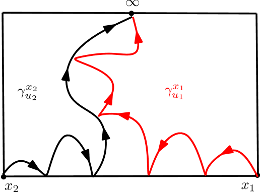
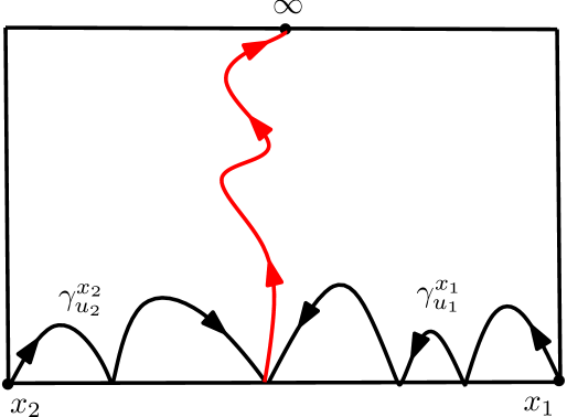
Theorem 1.1.4.
Suppose that is a on whose boundary value is piecewise constant. For each and , let be the level line of with height starting from . Fix .
-
(1)
If , then almost surely stays to the left of .
-
(2)
If , then may intersect and, upon intersecting, the two curves merge and never separate.
Remark 1.1.5.
Assume the same notations as in Theorem 1.1.4. Fix . We have the following facts about the intersection of the level lines and .
-
(1)
When , the level lines and do not intersect each other almost surely.
-
(2)
When , the Hausdorff dimension of the intersection is given by the following.
almost surely on the event .
In [MW16], the authors proved the Hausdorff dimension of the intersection of flow lines which corresponds to . The same proof works for the intersection of level lines.
The following theorem tells the reversibility of the level lines of .
Theorem 1.1.6.
Suppose that is a on whose boundary value is piecewise constant. Let be the level line of starting from 0 targeted at ; and be the level line of staring from targeted at 0. Then, on the event that the two paths do not hit the continuation thresholds before they reach the target points, the two paths and are equal (viewed as sets) almost surely.
This implies the reversibility of process. Suppose that is an process in starting from 0 targeted at . Then, conditioned on the event that the continuation threshold is not hit before reaches , we have that the time-reversal of has the law of process starting from targeted at (with appropriate weights and force points) conditioned on the event that the continuation threshold is not hit before it reaches . In particular, fix . Suppose that is an process in starting from 0 targeted at with two force points next to the starting point. Then the time-reversal of has the law of process in starting from targeted at 0 with two force points next to the starting point.
Finally, we state the result which is called the “target-independent” property of the level lines of .
Theorem 1.1.7.
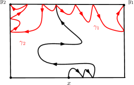
Suppose that is a on whose boundary value is piecewise constant. Fix three distinct boundary points . For , let be the level line of starting from targeted at ; define to be the first disconnecting time: is the inf of such that and are not on the boundary of the same connected component of . See Figure 1.1.3. Then, almost surely, the paths and coincide up to and including the first disconnecting time (modulo time-change); given , the two paths continue towards their target points independently.
1.2 Couplings between and
Note that paths can be viewed as level lines of GFF; and that is a collection of -type loops. It is natural to expect that the collections of level loops of correspond to . In this section, we will describe two couplings between and . Before this, we first recall a standard result about Brownian motion. Consider a one-dimensional standard Brownian motion . We take the reflected Brownian motion and it is well known that , if we decompose this at zero set of the Brownian motion , then this reflected Brownian motion can be decomposed into countably many Brownian excursions (a Brownian excursion is a Brownian path with and for ). Consider the local time process of the Brownian motion, it is increasing on zero set of the Brownian motion and is constant inside each excursion. If we parameterize these Brownian excursions by the local time process, then the sequence of these Brownian excursions is a Poisson point process. We can also reverse this procedure to construct a Brownian motion from a Poisson point process of Brownian excursions. Given a Poisson point process of Brownian excursions , there are two ways to reconstruct a Brownian motion:
-
(a)
Sample i.i.d. coin tosses for each excursion , let the excursion to be positive or negative according to the sign ; then concatenate these signed excursions. The process we get is a Brownian motion.
-
(b)
Concatenate all these excursions and get the reflected Brownian motion . Define the local time process of . Then the process has the same law as a Brownian motion.
In the following of this section, we will describe somewhat analogous pair of couplings between GFF and . The first coupling between GFF and is stated by Jason Miller and Scott Sheffield in 2011 and a proof can be found as a special case in [MWW13, Theorem 1.2].
Let be a in . For each loop , sample to be or with equal probability . We also call as the orientation of , i.e. (resp. ) corresponds to being oriented clockwise (resp. counterclockwise). All these orientations are sampled in the way that, given , they are conditionally independent. The the obtained sample is called with symmetric orientations.
Theorem 1.2.1.
Suppose that is a zero-boundary on and that is a with symmetric orientations in . There exists a coupling between and such that the following is true. Given , for each loop , the conditional law of restricted to the interior of , denoted by , is the same as with boundary value ; for different loops, the restrictions of the field are conditionally independent.
We refer to the coupling between GFF and CLE4 with symmetric orientations in Theorem 1.2.1 as the first coupling between and . As we can see, it can be viewed as the analog of the first reconstruction of Brownian motion from Brownian excursions.
In the current paper, we focus on another coupling between GFF and : the coupling between GFF and CLE4 with time parameter, which can be viewed as the analog of the second reconstruction of Brownian motion. with time parameter is a where each loop has a time parameter (precise construction will be recalled in Section 3.2). Roughly speaking, the time parameter for each loop is the counterpart of the local time for each excursion in the second reconstruction of Brownian motion. The main theorem is the following.
Theorem 1.2.2.
Suppose that is a zero-boundary on and that is a with time parameter in . There exists a coupling between and such that the following is true. Given , for each loop , the conditional law of restricted to the interior of , denoted by , is the same as with boundary value ; for different loops, the restrictions of the field are conditionally independent.
The second coupling between GFF and is stated by Scott Sheffield, Samuel Watson, and Hao Wu in 2012. The authors thank Scott Sheffield and Samuel Watson for allowing us to write up the details of the proof.
1.3 Relation to previous works and outline
We prove Theorems 1.1.1 to 1.1.7 in Section 2. Following is the outline of Section 2.
-
•
Section 2.1 is an introduction to chordal process.
- •
-
•
Sections 2.3 to 2.5 complete the proofs of Theorems 1.1.2 and 1.1.3. The proofs in these sections are similar to those in [MS16a, Section 4, Section 5, Section 6], whereas some part of the reasoning in [MS16a] does not apply to case. Thus, even though similar, we choose to rewrite and reorganize these proofs to treat case.
-
•
Section 2.6 completes the proof of Theorem 1.1.4. In [MS16a, Section 7.2], the authors prove a similar merging and monotonicity result for flow lines (i.e. for with ). In the current paper, we give a different proof for level line merging and monotonicity result based on the special property of the level lines: reversibility.
-
•
Section 2.7 completes the proofs of Theorems 1.1.6 and 1.1.7. The discussion about the reversibility of level lines of can be found in [SS13] for the setting that the curves are standard paths. We generalize this result to process. The discussion about reversibility for SLE paths can also be found in [Zha08, Zha10, Dub09b, MS16b, MS12] for different settings.
We prove Theorem 1.2.2 in Section 3. Following is the outline of Section 3.
-
•
Section 3.1 is an introduction to radial process.
- •
-
•
In Section 3.3, we introduce level lines of targeted at interior points (in contrast with the level lines targeted at boundary points studied in Section 2). We explain the monotonicity property and the target-independent property of the level lines targeted at interior points, which are analogous to Theorems 1.1.4 and 1.1.7 for the level lines targeted at boundary points.
- •
Our contribution in the current paper.
-
•
We summarize various properties of level lines of that start from boundary points and are targeted at boundary points (Section 2).
- •
-
•
We describe the behavior of level lines of that start from boundary points and are targeted at interior points (Section 3). We give a complete proof for the existence of the coupling between and with time parameter: Theorem 1.2.2. The close study on exploration process in Section 3 is an essential ingredient in the study of the level lines of emanating from an interior point in a forthcoming paper [WW15]. All this work plays an important role in a larger program on the study of conformal invariant metric on which includes [WW13, SWW16b, WW15, SWW16a].
In this paper, we focus on with piecewise constant boundary conditions. It is natural to wonder the situation of when the boundary condition is not piecewise constant. However, the techniques in this paper and the previous papers on the level lines of GFF do not apply directly to the general case. In [PW15], the authors study the properties of level lines of whose boundary condition is regulated without continuation threshold, and the important ingredient there is [KS12]. The results in Section 2 provide the platform for further studies there. As discussed in the introduction of [PW15], the properties of the level lines of when the boundary condition is not piecewise constant and does have continuation threshold is still open.
Acknowledgements. We thank Richard Kenyon, Jason Miller, Scott Sheffield, Samuel Watson, and Wendelin Werner for helpful discussions. H. Wu’s work is funded by NSF DMS-1406411.
2 Boundary emanating Level Lines of
2.1 Chordal
Suppose that is a continuous real function with . For each , define the function as the solution to Chordal Loewner Equation
This is well-defined as long as does not hit 0. Define
This is the largest time up to which is well-defined. Set
We can check that is a conformal map from onto normalized at and that, for each , as . The family is called the Loewner chain driven by . Here we collect some general results about chordal Loewner chain.
Proposition 2.1.1.
Suppose that is a continuous curve in from to with a continuous Loewner driving function . Then the set has Lebesgue measure zero.
Proof.
[MS16a, Lemma 2.5] ∎
Proposition 2.1.2.
Suppose that . Let be a continuous, non-crossing curve with . Assume that satisfies the following:
-
(1)
is contained in the closure of the unbounded connected component of ;
-
(2)
has empty interior in .
For each , let be the conformal map from the unbounded connected component of onto with . After reparameterization, solves the Loewner equation
with continuous driving function .
Chordal for is the Loewner chain driven by where is a 1-dimensional Brownian motion. Here are several basic properties of chordal SLE:
-
•
It is scale-invariant: For any , the process has the same law as itself.
-
•
It satisfies domain Markov property: For any finite stopping time , the process has the same law as itself where .
Proposition 2.1.3.
For all , chordal is almost surely generated by a simple continuous curve, i.e. there exists a simple continuous curve such that for all . Moreover, the curve is almost surely transient: .
Proof.
[RS05, Theorem 5.1] ∎
Fix and
Take the convention
Define
Definition 2.1.4.
Let be a standard Brownian motion. We will say that the process describe an process with force points if they are adapted to the filtration of and the following hold:
-
(1)
The processes and satisfy the following SDE on the time intervals on which does not collide with any of .
-
(2)
We have instantaneous reflection of off of the , i.e. it is almost surely the case that for Lebesgue almost all times we have that for each .
-
(3)
We also have almost surely that, for each ,
We define the continuation threshold to be the infimum of the values for which
Proposition 2.1.5.
Definition 2.1.4 uniquely determines a joint law for –each defined for all up to the continuation threshold. Under this law, the process is a continuous multidimensional Markovian process indexed by .
Proof.
[MS16a, Theorem 2.2]. ∎
Proposition 2.1.6.
Assume that
Then process is a continuous curve.
Proof.
Under the assumption that , for all , the curve can not hit the boundary and thus it is absolutely continuous with respect to , and then it is almost surely continuous. ∎
Proposition 2.1.7.
Suppose we are given a random continuous curve in from to whose Loewner driving function is almost surely continuous. Suppose is the corresponding Loewner chain and is the corresponding sequence of conformal maps. Set . Suppose that is the image of under . Let be the function defined in Theorem 1.1.1. Then and can be coupled with a standard Brownian motion to describe an process with force points up to the continuation threshold if and only if evolves as a Brownian motion when parameterized by the log of the conformal radius of seen from , for each fixed , until the time that is swallowed by .
Proof.
[MS16a, Theorem 2.6]. ∎
The following two propositions are results about the interacting behavior of SLE process with the boundary that we will use later in the paper.
Proposition 2.1.8.
Fix . Suppose that is an process with force points where . Set
Let be the first time that swallows .
-
(1)
Assume that, for some , we have that for ; and for . Then almost surely, as , accumulates at without hitting any other point in .
-
(2)
Assume that, for some , we have that for ; ; and for . Then almost surely, as , accumulates at a point in without hitting any other point in .
Proof.
[Dub09a, Lemma 15]. ∎
Proposition 2.1.9.
Fix . Suppose that is an process with force points where . Set
Assume that, for some stopping time , is almost surely generated by a continuous curve . Then almost surely does not intersect any interval such that
Proof.
[MS16a, Lemma 5.2 and Remark 5.3]. ∎
2.2 The Zero-Boundary
Suppose that is a proper domain with harmonically non-trivial boundary (i.e. a Brownian motion started at a point in hits almost surely.) For , we denote by the inner product of :
where is the Lebesgue area measure. Denote by the space of real-valued smooth functions which are compactly supported in . This space has a Dirichlet inner product defined by
Denote by the Hilbert space completion of .
The zero-boundary on is a random sum of the form , where the are i.i.d. one-dimensional standard Gaussians (with mean zero and variance 1) and the are an orthonormal basis for . This sum almost surely does not converge within ; however, it does converge almost surely within the space of distributions— that is, the limit almost surely exists for all , and the limiting values, denoted by , as a function of is almost surely a continuous functional on . For any , let , and define
Then is a mean-zero Gaussian with variance
The zero-boundary on is the only random distribution on with the property that, for each , is a mean-zero Gaussian with variance .
When is fixed, let be the harmonic extension to of the function of on given by . Then the Green’s function in the domain is given by
| (2.2.1) |
For any , define on by
This is a smooth function in whose Laplacian is and whose boundary value is zero on . We point out that the Green’s function is conformally invariant: if is a conformal map on , then, for any , we have
| (2.2.2) |
Note that, for any , we have that
For any deterministic open subset , there is a natural inclusion of into by . We can see that admits the -orthogonal decomposition
| (2.2.3) |
where is the space of functions in that are harmonic in . The reason is the following. For any , let be the function that equals on and be harmonic in and let . Then , and .
The decomposition in Equation (2.2.3) leads to a decomposition of the on :
| (2.2.4) |
where and are distributions on such that, for any ,
Clearly, and are independent.
For any distribution on , we define the restriction of to , denoted by , to be restricted to the functions that are compactly supported in . If is a zero-boundary on , then is a zero-boundary on and is almost surely harmonic. Thus, the conditional law of given is that of the zero-boundary on plus the harmonic extension of to . This is called “domain Markov property” of the .
Suppose that is a piecewise continuous function on , and that is the harmonic extension of to . We define the on with mean to be the sum of a zero-boundary plus . Sometimes, we use the term “the with boundary value ” to refer to the with mean .
Proposition 2.2.1.
Suppose that are simply connected domains with . For , let be a zero-boundary on and be harmonic on . Fix a simply connected open domain .
-
(1)
If for , then the law of
are mutually absolutely continuous.
-
(2)
Suppose that there is a neighborhood of the closure such that , and that tends to zero as one approaches points in the sets . Then the laws of
are mutually absolutely continuous.
Proof.
[MS16a, Proposition 3.2]. ∎
Suppose that is a simply connected domain, and that is a random closed subset of . For , let denote the closed set containing all points in whose distance from is at most . Let be the smallest -algebra in which and the restriction of to the interior of are measurable. Let . Intuitively, this is the smallest -algebra in which and the values of in an infinitesimal neighborhood of are measurable.
Proposition 2.2.2.
Suppose that is a random variable which is a coupling of an instance of the and a random closed subset . Then the following are equivalent:
-
(1)
For any deterministic open set , we have that, given the orthogonal projection of onto , the event is independent of the orthogonal projection of onto . In other words, the conditional probability of given is a measurable function of the orthogonal projection of onto .
-
(2)
Given , the conditional law of is that of where is a zero-boundary on and is an -measurable random distribution which is almost surely harmonic on .
Proof.
[SS13, Lemma 3.9]. ∎
We say a random closed set coupled with an instance of is a local set for if one of the equivalent items in Proposition 2.2.2 holds. For any coupling of and , we use the notation to describe the conditional expectation of given . When is local, is the described in Item (2) in Proposition 2.2.2. We use the notation to refer to and also say that is the conditional expectation of given and . By convention, we write the mean of .
Proposition 2.2.3.
Suppose that is a and are random closed subsets of and that and are couplings for which are local. Let denote the random closed subset of which is given by first sampling , then sampling conditionally independent given , and then taking the union of and . Then is also local for . Moreover, given , the conditional law of is given by plus an instance of zero-boundary on .
Proof.
[SS13, Lemma 3.10]. ∎
Proposition 2.2.4.
Let be connected local sets which are conditionally independent and . Then is almost surely a harmonic function in that tends to zero along all sequences of points in that tend to a limit in a connected component of (which consists of more than a single point) or that tend to a limit on a connected component of (which consists of more than a single point) at a point that is a positive distance from either or .
Proposition 2.2.5.
Let be connected local sets which are conditionally independent and . Suppose that is a -measurable connected component of such that almost surely. Then almost surely, given . In particular, is independent of the pair given .
Proof.
[MS16a, Proposition 3.7]. ∎
Proposition 2.2.6.
Let be a on and suppose that is an increasing family of closed sets such that is local for for every -stopping time ; and, for a fixed , that is almost surely continuous and monotonic in . Then has a modification which is a Brownian motion when parameterized by
up until the first time that accumulates at . In particular, has a modification which is almost surely continuous in .
Proof.
[MS16a, Proposition 6.5]. ∎
We close this section by the proof of Theorem 1.1.1. To simplify the notations, we only prove the conclusion for the case when there is only one right force point and one left force point. The general case can be proved similarly. We state it as a proposition.


Proposition 2.2.7.
Fix and . Suppose that the process describe an process with force points . Let be the corresponding Loewner chain and let be the corresponding sequence of conformal maps, and set . There exists a coupling where is a zero-boundary on such that the following domain Markov property is true. Suppose that is any finite stopping time less than the continuation threshold for . Let be the function which is harmonic in with boundary values
Define, for ,
Then, given , the conditional law of is equal to the law of .
Proof.
For , define
where is the continuation threshold. From Proposition 2.1.6, when , we know that is generated by a continuous curve, and is exactly this continuous curve. We will prove that, for general and , the process is also generated by a continuous curve up to and including the continuation threshold. But we do not assume the continuity of SLE process in the proof of Theorem 1.1.1. In fact, the proof of the continuity for general , that we will show later, based on the coupling between and the Loewner chain of in Theorem 1.1.1.
First, we analyze the function . It is well-defined when , and when is swallowed by , we define to be the limiting value of as approaches the first time at which is swallowed by . Note that, for fixed , the function is harmonic in , and it is also harmonic in the finite connected component of with certain boundary value, see Figure 2.2.1. From Proposition 2.1.7, we know that is a continuous martingale up to the first time that is swallowed by . Suppose that is a Möbius transformation of such that is a conformal map from onto that preserves . Define
which is the log of the conformal radius of seen from . We have that
Second, we analyze the product for . Recall that the Green’s function of the upper-half plane is given by
Fix , define
and when at least of one of is swallowed by , we define to be the limiting value of when approaches the first time at which at least one of is swallowed. Note that, when , is the Green’s function of the domain ; when are not in the same connected component of , becomes zero; and when are in the same connected component of , is just the Green’s function of that connected component.
We will show that is a continuous martingale up to the first time that at least one of is swallowed. Note that
By Itô’s formula,
Thus and is a local martingale. Note that and are continuous and bounded, and that is continuous and non-increasing in . These imply that is a continuous martingale.
Third, for any test function , define
and we will explain that is a continuous martingale and
| (2.2.5) |
Since is a continuous martingale and is bounded uniformly over , by Fubini’s theorem, the integral is also a bounded continuous martingale. To show Equation (2.2.5), it suffices to show that is a martingale. Note that
| (2.2.6) |
We know that is a continuous martingale; and that are bounded (uniformly over ); and that is non-increasing in . Thus, by Fubini’s theorem again, the right-hand side of Equation (2.2.6) is a continuous martingale.
Finally, we will explain how to construct the coupling that satisfies the domain Markov property. Define, for ,
The limit exists almost surely for fixed since is a bounded martingale. Define, for and which is non-negative,
The limits exist because that and are non-increasing functions in . Let equal to plus a sum of independent zero-boundary ’s, one in each connected component of . The marginal law of is the same as a zero-boundary and the reason is the following. For any test function which is non-negative, and any , we have that
where the last equality is due to the fact that is a continuous bounded martingale with mean and quadratic variation . To complete the proof, we need to explain that the coupling satisfies the domain Markov property. In fact, for any test function , the conditional law of given is the same as a Gaussian with mean and variance . ∎
If and a are coupled as in Theorem 1.1.1, we say that the path , where is the continuation threshold of , is the level line of . Generally, for any simply connected domain with two distinct boundary points and and a fixed number , we say that the path is the level line of a with height in starting from targeted at if is the level line of where is any conformal map from onto that sends to and to .
2.3 Proof of Theorems 1.1.2-1.1.6—non-boundary-intersecting case
In this section, we mostly work in the horizontal strip:
Write the upper-boundary and the lower-boundary of in the following way:
Lemma 2.3.1.
Suppose that is a on the strip whose boundary value is as in Figure 2.3.1(a) and let be the level line of starting from . If , then almost surely accumulates at ; if , then almost surely accumulates at . In both cases, almost surely does not hit . If , then almost surely accumulates in ; and after it accumulates in , can be continued when it is targeted to or —i.e. the continuation threshold is not hit when first accumulates in .
Proof.
Case 1: . Let be the conformal map from onto which sends 0 to 0, to , and to . Then has the law of with force point at where . From Proposition 2.1.8, we know that accumulates at without hitting the boundary.
Case 2: . This case can be proved similarly.
Case 3: . We have the following two observations:
-
(a)
Let be the conformal map from onto that sends 0 to 0, to 1, to . Then has the law of process with force point 1 where . From Proposition 2.1.8, we know that accumulates in . This implies that accumulates in or before reaches .
-
(b)
Let be the conformal map from onto that sends 0 to 0, to , to . Then has the law of process with force point where . From Proposition 2.1.8, we know that accumulates in . This implies that accumulates in or before reaches .
Combining these two facts, we know that almost surely accumulates in before reaches . ∎


Remark 2.3.2.
The conclusions in Lemma 2.3.1 hold more generally when the boundary data of on is piecewise constant, and is at least to the right of 0 and is at most to the left of 0. Furthermore, the level line is almost surely a continuous curve until it first accumulates in .
Proof.
From Proposition 2.1.8, we know that almost surely does not hit after time 0. Thus, up to the first time that accumulates in , the law of is absolutely continuous with respect to the law of . Therefore is continuous up to . ∎
Lemma 2.3.3.
Suppose that is a on the strip whose boundary value is as in Figure 2.3.1(b) and let be the level line of starting from . If , then almost surely exits at without otherwise hitting .
Proof.
Let be the conformal map from onto that sends 0 to 0, to 1, and to . Put . Then has the law of with force points where
From Proposition 2.1.8, we know that almost surely accumulates at without otherwise hitting the boundary. ∎
Remark 2.3.4.
The conclusion in Lemma 2.3.3 holds more generally when the boundary data of is piecewise constant, and is
Furthermore, the level line is almost surely a continuous curve from 0 to .
Lemma 2.3.5.
Suppose that is a on the strip whose boundary value is as in Figure 2.3.1(c) and let be the level line of starting from . If and , then almost surely exits in without otherwise hitting .
Proof.
Let be the conformal map from onto that sends 0 to 0, to 1, and to . Put
Then has the law of with force points where
Thus will first accumulates in without hitting other boundary points by Proposition 2.1.8. ∎
Remark 2.3.6.
The conclusion in Lemma 2.3.5 holds more generally when the boundary data of is piecewise constant, and is
Furthermore, the level line is almost surely a continuous curve until it first accumulates in .
Proposition 2.3.7.
Suppose that is a on the strip whose boundary value is as in Figure 2.3.2(a). Let be the level line of starting from 0 and be the level line of starting from , and assume that the triple are coupled so that and are conditionally independent given . Then almost surely and (viewed as sets) are equal. In particular, the level line is almost surely determined by .

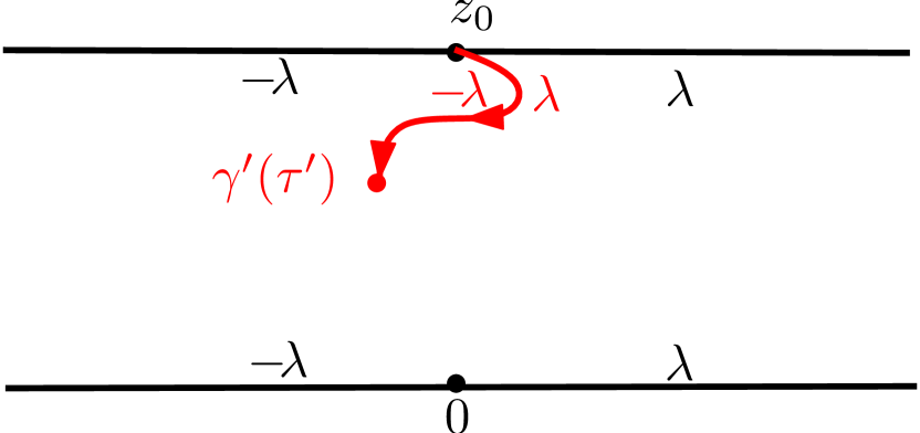
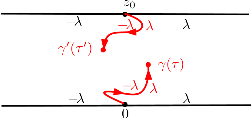
To prove Proposition 2.3.7, we first prove the following lemma.
Lemma 2.3.8.
Suppose the same assumption as in Proposition 2.3.7. Let be any -stopping time. Then, given , the level line almost surely first exits at .
Proof.
Given , denote by the restriction of to . Since and are coupled as in Theorem 1.1.1, we know that the conditional law of given is the same as a on with boundary data as in Figure 2.3.2(b).
We argue that, given , the path and the field are coupled so that is the level line of . Assuming this is true, then, from Lemma 2.3.3, we know that almost surely exits at which implies the conclusion. Thus we only need to show that, given , the path and the field are coupled so that is the level line of .
Suppose is any -stopping time. We know that is a local set for , that is a local set for , and that and are conditionally independent given . From Proposition 2.2.3, we know that the union is also a local set for ; furthermore, given and , and on the event , the conditional law of is the same as a in with boundary data as in Figure 2.3.2(c). This implies that, given , the path and the field are coupled so that is the level line of up until the first time that hits . This completes the proof. ∎
Proof of Proposition 2.3.7.
From Lemma 2.3.8, we have almost surely that hits for the first time at . Since this holds for any -stopping time , we know that hits a dense countable set of points along (in reverse chronological order). By symmetry, hits a dense countable set of points along . Since both and are continuous simple curves, the two paths (viewed as sets) are equal. ∎
Remark 2.3.9.
From Proposition 2.3.7 and Remark 2.3.9, we finish the proof of Theorems 1.1.2 to 1.1.6 for the case that the level lines are non-boundary-intersecting. We record these results in the following proposition.
Proposition 2.3.10.
Suppose that is a on whose boundary value is piecewise constant, and is
Let be the level line of starting from 0 targeted at and be the level line of starting from targeted at 0. Then we have the following conclusions.
-
(1)
The level line is almost surely determined by .
-
(2)
The level line is almost surely continuous and transient.
-
(3)
The level lines and are equal.
Proof.
We only need to explain the transience. Let be any -stopping time that is positive and finite. From Remark 2.3.9, we know that, given , the level line first exits at and then merges with afterwards. Therefore is transient by the continuity of at time . ∎
In this section, we will consider the relation between two level lines of the same . Suppose that is a , for any , we define the level line of with height to be the level line of . We will show that the level lines of enjoy the same monotonicity property as if were a smooth function. Namely, if and is the level line of with height for . Then almost surely lies to the right of .
Proposition 2.3.11.
Suppose that is a on with boundary data as in Figure 2.3.4(a). Assume that and let be the level line of starting from . Fix such that
| (2.3.1) |
and let be the level line of with height starting from 0 and stopped at the first time that it accumulates in . If , then almost surely passes to the left of ; if , then almost surely passes to the right of .
To prove the proposition, we need the following lemma.
Lemma 2.3.12.
Suppose that is a on whose boundary data is as in Figure 2.3.3. Let be the level line of starting from 0. If is almost surely continuous for some -stopping time , then almost surely.
Proof.
This is a direct consequence of Proposition 2.1.9. ∎


Proof of Proposition 2.3.11.
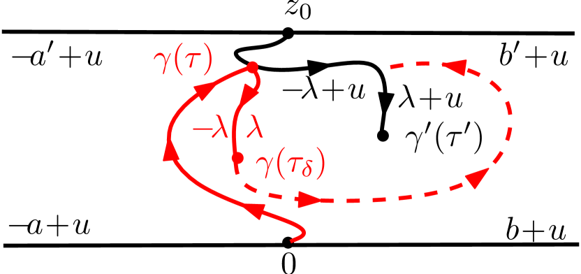
We only need to show the result for . Let be the level line of starting from , and be the level line of with height starting from 0. The hypothesis that implies that almost surely first exits at 0 without hitting any other boundary point (except and ) and is almost surely continuous. The hypothesis in Equation (2.3.1) implies that almost surely accumulates in or tends to before hitting after time 0 and is almost surely continuous up to the first time that it hits . Let be any -stopping time before it hits 0. Let be restricted to . Then, given , the conditional law of is the same as a with boundary data as in Figure 2.3.4(b). Furthermore, is the level line of .
We say the left (resp. right) side of the union of the left (resp. right) side of and the part of that is to the left (resp. right) of . From Lemma 2.3.5 and Remark 2.3.6, we know that almost surely exits on the left side of , say at time , or does not hit .
We will argue that is almost surely to the right of . If is in the part of that is to the left of , then we are done. If this does not hold, then is to the left of , and therefore hits the left side of at time and, after time , the path wraps around and then hits the right side of . See Figure 2.3.4(c). Let be the first time after that is in the right connected component of and (set if this never happens). Then for small enough, the probability of the event is positive. Given , the conditional law of restricted to the right connected component of is the same as a with boundary value as in Figure 2.3.4(c). Furthermore, is the level line of this field. From Lemma 2.3.12, will never hits the right side of , contradiction. ∎
Proposition 2.3.13.
Suppose that is a on with boundary data as in Figure 2.3.4(a). Assume that . Fix such that
For , let be the level line of with height starting from 0 and let be the first time that accumulates in . Then, almost surely, lies to the left of . We emphasize that there is no restriction for the boundary data of on .
Proof.
We first assume that and . By replacing with , we may assume that . Let be the level line of starting from . From Proposition 2.3.11, we know that almost surely stays to the left of . We also know that the range of is the same as the range of . These imply the conclusion.
Now we treat the case when the boundary data of on is general. Fix , for , let be the first time that gets within distance of . It suffices to show that almost surely lies to the left of for every .
Let be a on whose boundary data is the same as on and, on , is at most to the left of and is at least to the right of . For , let be the level line of with height starting from 0. On the one hand, from the above analysis, almost surely lies to the left of . On the other hand, the laws of and are mutually absolutely continuous, see Proposition 2.2.1. Combining these two facts, we know that almost surely lies to the left of . ∎
Corollary 2.3.14.
Suppose that is a on whose boundary data is on and on . Assume that . Fix such that
For , let be the level line of with height starting from 0. Then almost surely lies to the left of .
Suppose that is a on whose boundary value is as in Figure 2.3.5(a). For each , let be the level line of with height starting from 0. Fix and assume that are large enough so that Corollary 2.3.14 is applicable to and . We know from Corollary 2.3.14 that almost surely lies to the right of . The purpose of the rest of this section is to calculate the conditional mean of given both and , and to show that the Loewner driving function of , viewed as a path in the right connected component of , exists and is continuous, and likewise when the roles of and are swapped. We emphasize that, in this section, the results will be for paths which do not intersect the boundary where we have the almost sure continuity of the level lines at this point.
Lemma 2.3.15.
Suppose that are continuous paths such that, for each , we have that
-
(1)
is a local set for for any -stopping time ;
-
(2)
is almost surely determined by .
Suppose that is a stopping time for and, for each , inductively, let be a stopping time for the filtration generated by and . Then is a local set for and is almost surely determined by .
Proof.
For , set . Fix open. We are going to prove that the event is almost surely determined by and that, on the event , the set is almost surely determined by . We will prove this by induction on the number of the paths. The hypotheses for imply that this is true for . Suppose the result holds for paths for fixed. We will show that it holds for paths.
Let be the first time that hits . The hypotheses of imply that is almost surely determined by . Note that
-
(a)
;
-
(b)
the event is almost surely determined by and (since is a -stopping time);
-
(c)
the event is determined by , and on the event , the set is almost surely determined by .
Combining these three facts, we have that, on the event , the event is almost surely determined by . Therefore, the event is almost surely determined by ; moreover, on the event , since and are almost surely determined by , is also almost surely determined by . This completes the proof of the induction step. ∎
In the rest of this section, we set
Proposition 2.3.16.
Suppose that is a on whose boundary value is as in Figure 2.3.5(a). Fix an -stopping time . Let be any connected component of . Then, given , the conditional law of is the same as a with mean which is harmonic in with certain boundary value that will be described in the following. There are three types of and we will describe the boundary value of one by one, see Figure 2.3.5(b).
-
(1)
is the connected component that stays to the left of . Then is on and to the left of .
-
(2)
is any connected component between and . Then is to the right of and to the left of .
-
(3)
is the connected component whose boundary contains . Then is to the right of , to the left of , to the right of , and on .

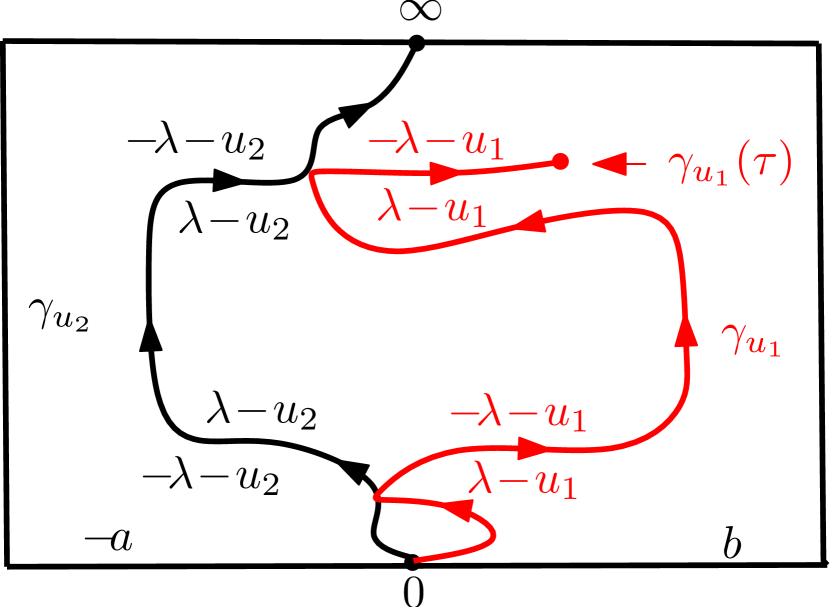
.
Proof.
From Lemma 2.3.15, we know that is a local set for . Since and are continuous, the connected components of and of consist of more than a single point. For , let be the range of , and set .
First, assume that and is the connected component to the left of or the connected component to the right of . We only need to explain the result for that is the connected component to the left of . Note that and are local sets determined by . Apply Proposition 2.2.5 to and , we have that almost surely given . Therefore, given , the conditional mean agrees with almost surely.
Second, assume that and is any connected component between and . Then has two special points, say and , which are contained in . For any fixed point (resp. ) other than , from Proposition 2.2.4, we know that (resp. ) tends to zero along any sequence in which converges to . Thus agrees with on . Then we need to show that also agrees with at and .
Assume and with . Proposition 2.2.6 implies that has a continuous modification in since that is local for any -stopping time and that is continuous. The continuity of in implies that has the same boundary behavior as near since that the boundary data of agrees with as . This leaves us to deal with the boundary behavior near .
Let be the level line of with height starting from , and let be the range of . Then almost surely . Apply Proposition 2.2.5 to the sets and , we have that almost surely given . An analogous continuity argument implies that has the same boundary behavior as near . Consequently, also has the same boundary behavior as near .
Third, assume that and is the connected component to the left of . Apply Proposition 2.2.5 to and , which are local and are determined by , we have that given . This implies that agrees with .
Fourth, assume that and is any connected component between and . Apply Proposition 2.2.5 to and , we have that given . Since agrees with , also agrees with .
Finally, assume that and is the connected component whose boundary contains , see Figure 2.3.5(c). Take a point on . If is at positive distance from , by applying Proposition 2.2.4 to the sets and , we know that tends to zero along any sequence in that converges to , thus agrees with at . If is at positive distance from , by applying Proposition 2.2.4 to the sets and , we know that tends to zero along any sequence in that converges to , thus agrees with at . If is not in the previous two cases, then a similar continuity argument as above will imply that agrees with at . ∎
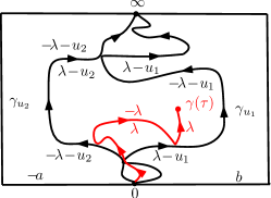
Remark 2.3.17.
The rest of this section is to establish the existence and continuity of the Loewner driving function for viewed as a path in the right connected component of . We will use Proposition 2.1.2.
Proposition 2.3.18.
Let be a conformal map from the right connected component of onto with and . Then has a continuous Loewner driving function as a path in from to .
Proof.
Since is continuous, the right connected component of , denoted by , is almost surely a Jordan domain. Thus extends as a homeomorphism from onto , and is almost surely a continuous curve in from 0 to . We will check the two criteria in Proposition 2.1.2.
Proof of Condition (1). The only way this could fail is if the following occurs. After intersecting , say at time , enters a bounded connected component of , denoted by . Since lies to the right of , this would force to have a self-intersecting upon exiting . This contradicts with the fact that is simple.
Proof of Condition (2). It suffices to show that the set of times such that is contained in the range of is nowhere dense in almost surely. Since is closed, we only need to show that the event has probability zero. We prove by contradiction. Suppose that . Let , and let be an -measurable random variable taking values in such that, on the event , is almost surely contained in an open interval of . On the event , since and are simple, we can find a sequence in the connected component that is to the left of converging to . Since that is connected and contains more than a single point, and that is at positive distance from , from Proposition 2.2.4, we know that converges to both and , contradiction. ∎
Remark 2.3.19.
[Three level lines] Suppose that , and . A statement analogous to Proposition 2.3.18 also holds for the path given and . Let be any connected component of which lies between and and let be the first and the last points on traced by . Let be a conformal map from onto with and . Then almost surely has a continuous Loewner driving function as a curve in .
2.4 Proof of Theorem 1.1.2—general case
In this section, we will first prove Theorems 1.1.2 to 1.1.6 in the special case of two force points and with weights . Then by an induction argument, we will complete the proof of Theorem 1.1.2 for multiple force points case.


We will work in the setting of Remark 2.3.17 and Remark 2.3.19. Suppose that is a on whose boundary data is as depicted in Figure 2.4.1(a) and assume that are large enough so that all the level lines we will consider do not intersect the boundary. Fix . For , let be the level line of with height starting from 0 and let be the level line of starting from 0. From Proposition 2.3.7 and Corollary 2.3.14, we know that , , are all almost surely continuous and are determined by , that stays to the right of , and that stays to the right of . Fix a connected component of which lies between and . Let be the first point in traced by and be the last point. Let be the restriction of to and let be the restriction of to the time interval in which it takes values in . Let be any conformal map from onto that sends to 0, to . Note that, by the continuity of and , the map can be extended as a homeomorphism from onto , and is almost surely a continuous curve in from to with continuous Loewner driving function, see Figure 2.4.1(b). Define
Lemma 2.4.1.
We have that has the law of process with force points where
Moreover, is almost surely continuous with and are coupled as in Theorem 1.1.1.
Proof.
First, we show that is a local set for for every -stopping time . Let be the time that , and define
From Remark 2.3.17, we know that is a local set for and is determined by ; and that, given , the conditional law of is the same as a on whose boundary data is as depicted in Figure 2.3.6. Thus, the conditional expectation restricted to given is harmonic with boundary data as depicted in Figure 2.3.6. Define
The above analysis implies that and are coupled so that, given , the conditional law of is the same as a on with mean which is harmonic in . This implies that is a local set for . This also implies that are coupled as in Theorem 1.1.1.
Second, we show the law of . Define, for and ,
By the continuity of , we know that the conformal radius is almost surely continuous. From Proposition 2.2.6, has a modification which is a Brownian motion when parameterized by minus the log of the conformal radius. Then Proposition 2.1.7 implies the law of . ∎
Lemma 2.4.2.
Almost surely, is determined by .
Proof.
Let (resp. ) be the restriction of to the connected component of that lies to the right of (resp. lies to the left of ). For the connected components of that lie between and , we can put an ordering by saying that for two connected components if and only if intersects before . Let (resp. ) be the restriction of to the connected components which come strictly before (resp. strictly after) in this ordering. We summarize the facts that we know in the following.
-
(a)
Given , the field is determined by .
- (b)
-
(c)
From Lemma 2.4.1, we know that is independent of .
Combining these three facts, to show the conclusion, we only need to show that, given , the couple is independent of . Assume and for .
First, we show that, given , the multiple is independent of . This can be obtained by applying Proposition 2.2.5 to the sets and .
Second, we show that, given , the triple is independent of . Applying Proposition 2.2.5 to the sets and , we know that, given , the triple is independent of . In particular, given , the triple is independent of .
Finally, we show that, given , the couple is independent of . By a similar analysis as in the second step, we know that, given , the triple is independent of (by considering the level line of starting from which merges with almost surely.) In particular, the couple is independent of . This completes the proof. ∎
By combining Lemma 2.4.1 and Lemma 2.4.2, we have obtained Theorems 1.1.2 to 1.1.6 in the special case of process with force points . We record it in the following proposition.
Proposition 2.4.3.
Suppose that is a on whose boundary value is on and is on . Assume that
Let be the level line of starting from 0 targeted at and let be the level line of starting from targeted at . Then we have the following conclusions.
-
(1)
The level line is almost surely determined by .
-
(2)
The level line is continuous and transient.
-
(3)
The level lines and are equal.
Proof.
We only need to show that and are equal. Suppose that is a on whose boundary data is on and on . Assume that and satisfy
Set
For , let be the level line of with height starting from 0. Let be the level line of starting from 0 and be the level line of starting from . We know that stays to the right of and that stays to the right of . From Proposition 2.3.7, almost surely merges with .
Given , let be any connected component of that lies between and and let be the first point on traced by and be the last point. Let be any conformal map from onto that sends to and to . Define
From Lemma 2.4.1, we know that is the level line of starting from 0 and that is the level line of starting from . From the above analysis, merges with . This completes the proof. ∎
Remark 2.4.4.
The conclusions in Proposition 2.4.3 also hold when the boundary value of the is on and is piecewise constant, and is at most on .
The technique we use to prove Proposition 2.4.3 can be applied to multiple level lines, we obtain as a consequence the following proposition.
Proposition 2.4.5.
Suppose that is a on whose boundary data is as depicted in Figure 2.4.1(a). Fix heights and assume that
For , let be the level line of with height starting from 0. Then almost surely lies to the right of . Moreover, given , the curve has the law of independently in each connected component of that lie to the right of . Similarly, given , the curve has the law of independently in each connected component of that lie to the left of .
Remark 2.4.6.
The conclusion in Proposition 2.3.13 also holds when we replace the restriction on by the following:
Proof of Theorem 1.1.2.
We will now complete the proof of Theorem 1.1.2. Namely, we will show that level line , whose law is , of the is almost surely determined by .
Write
We are going to prove the result by induction on and . We may assume by possibly adding zero weight force points. By Proposition 2.4.3, the conclusion holds when . Let be the Loewner chain of and be the sequence of centered conformal maps . Assume that the conclusion holds for some . We are going to prove that the conclusion holds for left force points and right force points. Let be the first time that accumulates in (set if this never happens).
First, we explain that is almost surely determined by . Let be the on whose boundary data is the same as on and is on ; and let be the Loewner chain of the level line of . Note that has left force points and right force points. For , let (resp. ) be the first time that (resp. ) gets within distance of . Define to be the open set obtained by removing from the points that are within distance of . It suffices to show that is almost surely determined by . Note that
-
(a)
From the induction hypothesis, we have that is almost surely determined by .
-
(b)
From Proposition 2.2.1, we have that and are mutually absolutely continuous.
Combining these two facts, the set is almost surely determined by as desired.
Note that if is the continuation threshold, then we are done.
Next, we assume that is not the continuation threshold and we explain that is almost surely determined by . Suppose that the rightmost point of is contained in . Then the conditional law of given is an process in from 0 to where
By the induction hypothesis, we know that is almost surely determined by , hence it is determined by given . This implies the conclusion. ∎
2.5 Proof of Theorem 1.1.3—general case
We will complete the proof of Theorem 1.1.3—the continuity of process—by extending the special case proved in Proposition 2.4.3.
Remark 2.5.1.
Suppose that is an process, we have the following observations.
-
(1)
is almost surely continuous when it is away from the boundary .
-
(2)
When hits , say at time , between force points before the continuation threshold is hit, from the absolute continuity in Proposition 2.2.1, we know that locally evolves like an process with one force point of weight (since is not the continuation threshold). Therefore, is continuous at time .
Combining these two facts, to get the continuity of , we need to rule out pathological behavior when interacts with a force point or hits the continuation threshold.
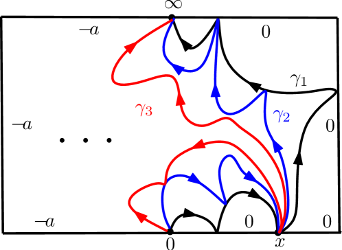
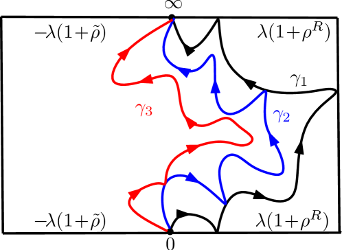
Lemma 2.5.2.
Suppose that is an process with force points where . Then the Lebesgue measure of is almost surely zero. In particular, for any , the probability that hits is zero.
Proof.
Fix . We only need to show that the probability that hits is zero.
First, we show that there exists some such that the probability that hits is zero. Suppose that is a on whose boundary data is on and on , see Figure 2.5.1(a). Since , we can pick so that
Fix . For , set and let be the level line of with height starting from 0. For , set
From Proposition 2.4.5, we have the following facts.
-
(a)
For , the marginal law of is .
-
(b)
For , given , the conditional law of is .
From the scale-invariance of process, we know that, for any fixed on the right part of the boundary, the probability that process hits is which is independent of . Thus
By the choice of , we know that , therefore . Thus there exists some such that where .
Next, we show the conclusion for general . Fix . Suppose that is a on whose boundary value is on and is on , see Figure 2.5.1(b). Set
For , let be the level line of with height starting from 0. From Proposition 2.4.5, we have the following facts.
-
(a)
Given , the conditional law of is .
-
(b)
Given , the conditional law of is .
-
(c)
The marginal law of is .
Since , we know that the probability that hits is zero. From the choice of , we know that, given , the probability that hits is zero. Combining these two facts, we know that the probability that hits is zero. Consequently, given , the probability that hits is also zero. This completes the proof. ∎
Suppose that is a on whose boundary value is on and on . Fix heights and assume that
| (2.5.1) | ||||
| (2.5.2) |
Let be the level line of with height starting from 0 and let be a -stopping time. For each , we inductively let be the level line of given with height starting from and let be a -stopping time. The restriction in Equation (2.5.1) guarantees that does not hit the continuation threshold when it hits and the restriction in Equation (2.5.2) guarantees that does not hit the continuation threshold when it hits itself. We call a height-varying level line of starting from 0 with heights with respect to the height change times . By Theorem 1.1.2 and an induction argument, we know that is almost surely determined by .
Lemma 2.5.3.
Suppose that is a on whose boundary data is on and on . Fix heights and assume that
For , let be the level line of with height starting from 0. Let be the height-varying level line of with height change time . Then we have the following conclusions.
-
(1)
is almost surely continuous and .
-
(2)
almost surely passes to the right of and almost surely passes to the left of .
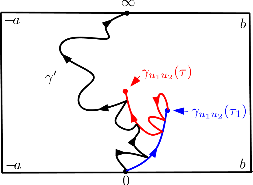
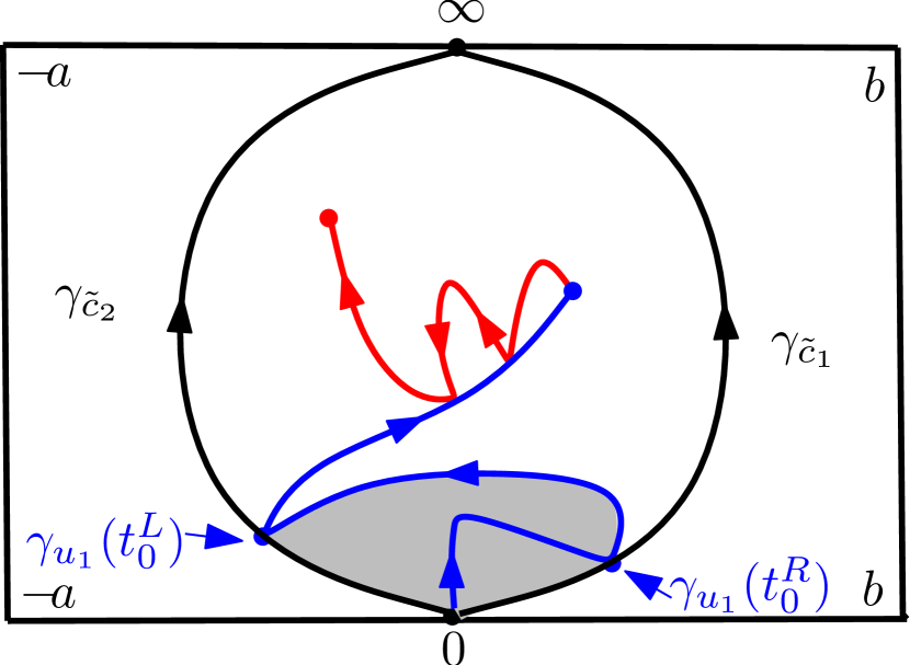
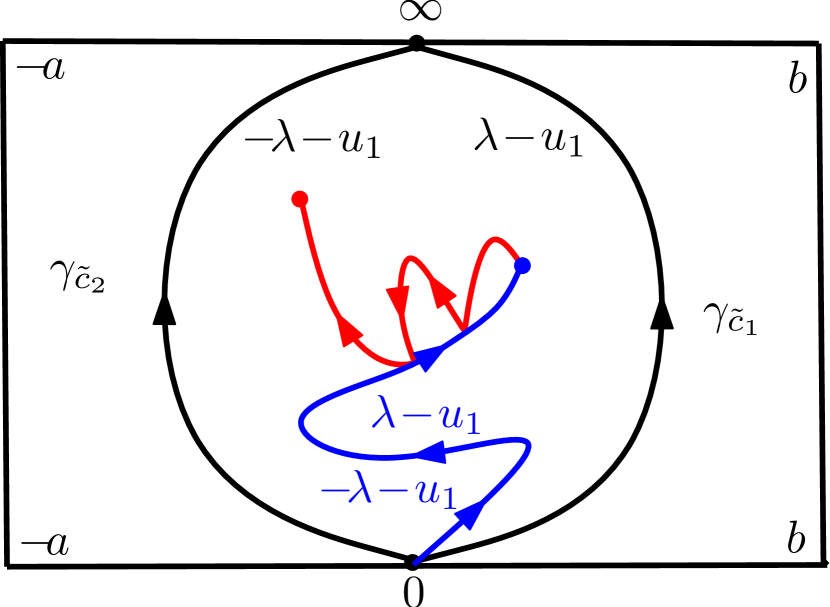
Proof.
We start by explaining that we only need to show the conclusions for large . Suppose that the conclusions hold for large , then we could apply the same argument used to prove Proposition 2.4.3 by conditioning on level lines with appropriately chosen heights and use the results of for large .
In the rest of the proof, we suppose that are large enough so that none of level lines that we use later hits the boundary (except at 0 and ). For , let be the first time after that gets within distance of the origin.
First, we explain that is continuous. Since that is the level line of with height , it is almost surely continuous. Given , let be the restriction of to , then the conditional law of is the same as a on whose boundary value is consistent with on , is to the right of and is to the left of . Furthermore, given , is the level line of with height . From Remark 2.5.1, it is continuous up to .
Second, we explain that almost surely passes to the right of . Symmetrically, we will have that almost surely passes to the left of . Suppose that is any -stopping time such that . Let be the level line of with height starting from . From Lemma 2.3.5 and Remark 2.3.6, we know that, given , the level line first exits through the left side of . Since that and are continuous, we can use the similar proof as the proof of Proposition 2.3.11 to show that stays to the right of , see Figure 2.5.2(a). Since the range of coincides with the range of , this implies the conclusion.
Third, we explain that does not hit the origin after time 0 and hence it is continuous by Remark 2.5.1. Choose constants satisfying
The restriction that guarantees that we are able to choose such . For , let be the level line of with height starting from 0. Note that stays between and , and that, given and , the conditional law of is with force points next to the starting point where
Define (resp. ) to be the sup of the times such that (resp. ) with the conventions that . By the choice of , we have that , see Figure 2.5.2(b). From the above analysis, we know that, stays between and for any . Thus, the path can not enter the bounded domain which is bounded by , and . This implies that the distance is strictly positive. Thus never hits the origin after time 0.
Fourth, we explain that almost surely stays between and . We have the following facts.
-
(a)
almost surely stays between and .
-
(b)
The distance is strictly positive.
Combining these two facts, we have that almost surely stays between and .
Finally, we explain the transience of , namely . Choose
For , let be the level line of with height starting from 0. We know that stays between and , see Figure 2.5.2(c); furthermore, given , the conditional law of is with force points next to the starting point where
From Proposition 2.4.3, we have the desired transience. ∎
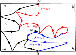
Lemma 2.5.4.
Suppose that is a on whose boundary data is on and on . Fix heights and assume that
Let be the level line of with height starting from 0. Let be the height-varying level line of starting from 0 with heights and height change time . Then, given , the conditional law of is process in the left connected component of where
Proof.
From Lemma 2.5.3, we know that is almost surely continuous and that almost surely stays to the left of . Define to be if and to be the last point in that is contained in if . Let be the conformal map from the left connected component of , denoted by , onto such that sends 0 to 0, to 1, and to . By the continuity of , the map can be extended as a homeomorphism from onto , and is almost surely a continuous curve in from 0 to with continuous Loewner driving function (by a similar argument as in the proof of Proposition 2.3.18). We can then use a similar argument as in the proof of Lemma 2.4.1 to show that the law of is in from 0 to with force points . ∎
Lemma 2.5.5.
Suppose that is a on whose boundary value is on , is on , and is on . Assume that
Let be the level line of starting from 0 targeted at and be the level line of starting from targeted at 0. Then we have the following conclusions.
-
(1)
The level line is almost surely continuous and transient; moreover, does not hit 1.
-
(2)
The level lines and are equal.
Proof.
Suppose that is a GFF on whose boundary value is on and is on . Assume that is large enough so that the level lines we will use later are non-boundary-intersecting. Set
Let be the level line of starting from 0 and be the level line of starting from . Let be the height-varying level line of starting from 0 with heights and height change time 1. Define to be if and to be the last point in that is contained in if . We summarize the relations between , and as follows.
-
(a)
By Proposition 2.3.10, the level line is continuous and transient; moreover, the paths and are equal.
-
(b)
By Lemma 2.5.3, the level line stays to the left of . Define to be the connected component of that has on the boundary. Let be the conformal map from onto that sends to , to , and to . Define which has the same boundary value as the in the statement of this lemma.
-
(c)
By Lemma 2.5.4, given , the path is the level line of and the path is the level line of .
Combining these three facts, given , we have that the level line is continuous and transient; moreover, the paths and are equal. Finally, we only need to show that does not hit . Take another level line of with height starting from 0. Then almost surely stays between and . If does not hit , neither does , then we are done. If hits , since the conditional law of given is an process with , we can use Lemma 2.5.2 to explain that almost surely does not hit . ∎
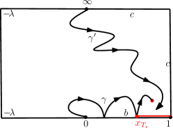
Lemma 2.5.6.
Suppose that is a on whose boundary value is on , is on , and is on . Assume that
Let be the level line of starting from 0 targeted at . Then, almost surely, does not hit 1 and is continuous and transient.
Proof.
If , the curve never hits the boundary after time 0, and we are done. In the following, we assume , then accumulates in by Proposition 2.1.8.
First, we show that does not hit 1 which implies the continuity by Remark 2.5.1. Let be the conformal map from onto that sends 0 to 0, to and to . Then the boundary value on is . By Lemma 2.3.1 and Remark 2.3.2, we know that accumulates in before reaches . This implies that first accumulates in the open interval .
Next, we show that is transient. Define to be the first time that accumulates in . Then, given , the conditional law of is with , which is transient by Proposition 2.4.3. This completes the proof. ∎
Lemma 2.5.7.
Suppose that is a on whose boundary value is on , is on , and is on . Assume that
Let be the level line of starting from 0 targeted at . Then, almost surely, does not hit 1 and is continuous.
Proof.
We only need to show that does not hit 1. We prove by contradiction. Assume that hits with positive probability, and, on this event, define to be the first time that gets within distance of 1. We have that is continuous up to . Let be the rightmost point of . Note that . Let be the level line of starting from . From Lemma 2.5.6, we know that is almost surely continuous and does not hit 1. By Lemma 2.3.12, we know that, given , the curve has to accumulate at or accumulate in , see Figure 2.5.4. This implies that has to get within distance of 1. Since that this holds for any and that is continuous, the curve will hits 1 with positive probability, contradiction. ∎


Lemma 2.5.8.
Suppose that is a on whose boundary value is as depicted in Figure 2.5.5(a). Assume that
Let be the level line of starting from 0 targeted at . Then, almost surely, is continuous, accumulates at before reaches , and does not hit other points in .
Proof.
Let be the conformal map from onto that sends 0 to 0, to 1, and to . Then is absolutely continuous with respect to process with force points where
Thus, by Lemma 2.5.7, we know that is continuous and does not hit which implies the conclusion. ∎
Lemma 2.5.9.
Suppose that is a on whose boundary value is as depicted in Figure 2.5.5(b). Assume that
Let be the level line of starting from 0 targeted at . Then, almost surely, accumulates in before reaches , is continuous up to the first time that it hits , and does not hit points in .
Proof.
Let be the first time that gets within distance of . Let be a on whose boundary value is the same as except that it is on . Let be the open set obtained by removing from all points that are within distance of . We have the following two observations.
-
(a)
The restriction of to is absolutely continuous with respect to the restriction of to by Proposition 2.2.1.
-
(b)
Let be the level line of starting from 0. From Lemma 2.5.8, we know that is continuous, it accumulates at , and it does not hit other points on .
Combining these two facts, we know that is continuous up to , does not reach before , and does not hit before . This is true for any and we could complete the proof by letting . ∎


Lemma 2.5.10.
Suppose that is a on whose boundary value is on , is on , and is on . Assume that
Let be the level line of starting from 0 targeted at and be the level line of starting from targeted at 0. Then, almost surely, the curves and are equal. In particular, is transient.
Proof.
Set . Let be the level line of with height starting from targeted at 1. We list the properties of and as follows.
- (a)
-
(b)
From Lemma 2.5.7, we know that is continuous and does not hit 1.
Combining these two facts and Lemma 2.5.9, we could apply a similar proof as the proof of Proposition 2.3.11 to show that almost surely stays to the left of . Furthermore, a similar proof as the proofs of Proposition 2.3.18 and Proposition 2.4.5 would show that the conditional law of given is where , see Figure 2.5.6(b). Define to be the left connected component of . We list the relations between , and as follows.
-
(a)
The curve stays to the left of and is the level line of given .
-
(b)
From Remark 2.4.6, we know that stays to the left of and is the level line of given .
Combining these two facts and Proposition 2.4.3, we know that, given , the curves and are equal. This implies the conclusion. ∎
We summarize several consequences of Lemmas 2.5.5 to 2.5.10. Suppose that is a on whose boundary data is on , is on , and is on . Assume that
Let be the level line of starting from 0, then the law of is with force points where
If and , the curve is continuous by Lemma 2.5.6; if , and , the curve is continuous by Lemma 2.5.7; if , and , then , thus is continuous by Lemma 2.5.5. In conclusion, we have the continuity of for all cases where . In fact, we have completed the proof of Theorems 1.1.3 and 1.1.6 for the case that there are two right force points with weights and satisfying
We record these conclusions in the following proposition.
Proposition 2.5.11.
Suppose that is a on whose boundary value is on , is on , and is on . Assume that
Let be the level line of starting from 0 targeted at and be the level line of starting from targeted at 0. The we have the following conclusions.
-
(1)
The level line is almost surely continuous and transient; moreover, it does not hit .
-
(2)
The level lines and are equal.
Remark 2.5.12.
The conclusions in Proposition 2.5.11 hold more generally when the boundary value of on is piecewise constant, and is at most .

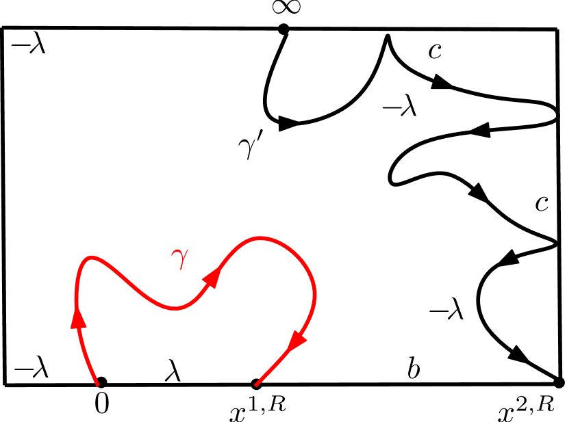
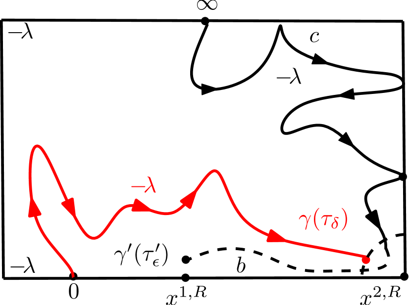
Lemma 2.5.13.
Suppose that or . Let be an process in from 0 to with force points where . Then is almost surely continuous up to and including the continuation threshold.
Proof.
Suppose that is a on whose boundary value is on , is on , is on , and is on , see Figure 2.5.7(a). Let be the level line of starting from 0, then its law is where
First, assume that . Let be the Möbius transformation of that sends 0 to 0, to , and to . Then has the law of with force points where
Thus is continuous and is transient by Proposition 2.3.10. This implies that is continuous up to and including the continuation threshold when it accumulates at .
Second, assume that . Let be the Möbius transformation of that sends 0 to 0, to , and to . Then has the law of with force points where
From Proposition 2.5.11 and Remark 2.5.12, we have that is continuous and transient. This implies that is continuous up to and including the continuation threshold when it accumulates at .
Finally, assume that . Define to be the first time that hits . By Remark 2.5.1, we know that is continuous. There are three cases for : case 1. ; case 2. ; case 3. . We analyze case by case.
Case 1. Suppose that . By Remark 2.5.1, we know that is continuous up to and including . Moreover, continues towards after . Thus the distance between and is positive and therefore the law of is absolutely continuous with respect to with force point where . By Proposition 2.5.11, we know that is continuous and transient.
Case 2. Suppose that . In this case, arrives its continuation threshold at and stops. We can prove that the distance between and is positive and the law of is then absolutely continuous with respect to the law of with force point where . By the first step, we know that is continuous up to and including the continuation threshold when it accumulates at .
Case 3. Suppose that and, in fact, we will show that this is impossible (or this happens with zero probability). Let be the level line of starting from targeted at . There are two possibilities: either reaches without hitting or it hits its continuation threshold when it accumulates in . In the former case, we can show that the distance between and is positive, therefore the law of is absolutely continuous with respect to SLE where . Thus is continuous and transient. Moreover, the path stays to the left of and the conditional law of given is SLE with force points where , see Figure 2.5.7(b). By the first step, we know that, given , the level line is continuous up to and including the continuation threshold when it accumulates at . This contradicts with . In the latter case, for , define to be the first time that gets within distance of and define to be the first time that gets within distance of . We have the following observations.
-
(a)
The path is continuous up to for any ; the path is continuous up to for any .
-
(b)
Given , the conditional law of is the level line of restricted to ; therefore can not hit the union of and the left side of . See Figure 2.5.7(c). Thus, given , the path has to get within distance of in order to get close to the interval .
Combining these two facts and letting go to zero, we have that accumulates at before hits , contradiction. ∎
Lemma 2.5.14.
Let be an process in from 0 to with force points where
Then is almost surely continuous up to and including the continuation threshold.
Proof.
From Proposition 2.5.11 and Lemma 2.5.13, we know that the conclusion holds when there are at most two force points. We prove the conclusion by induction. Suppose that the conclusion holds when there are at most force points, and we prove the continuity when there are force points:
Suppose that is a GFF on whose boundary value is on , is on , and is on for where
Let be the level line of starting from 0 targeted at , then the law of is with force points. Let be the first time that hits ; and set if this never happens. If , then the law of is absolutely continuous with respect to process with force points which is continuous up to and including the continuation threshold. Thus is continuous up to and including the continuation threshold.
In the following we suppose . For , define to be the first time that gets within distance of the interval .
First, we explain that is continuous up to . Let be the open set obtained by removing from all points that are within distance of . Let be the GFF on whose boundary value is consistent with outside and is on . Let be the level line of starting from 0 targeted at . Then has at most force points. We have the following two observations.
-
(a)
From Proposition 2.2.1, we know that the law of restricted to is absolutely continuous with respect to the law of restricted to .
-
(b)
From induction hypothesis, we know that is continuous.
Combining these two facts, we know that is continuous up to .
Second, we explain that, given , the conditional law of is continuous. Note that, given , the conditional law of is process with at most force points. Thus, given , the curve is continuous by induction hypothesis.
Finally, we explain the continuity of up to and including . Define
From the above analysis, we know that is continuous on the event . We only need to analyze the behavior of on the event . Note that, for , the event implies that has to accumulate in as . This holds for all on . The only possibility is that and accumulates at as . Let be the Möbius transformation of that sends 0 to 0, to , and to . Then has the law of SLE process with force points . On the event , from the above analysis, we have that does not hit the interval ; therefore it is absolutely continuous with respect to SLE which is continuous and transient. This implies that, on , the curve is continuous up to and including the time . This completes the proof. ∎
Proof of Theorem 1.1.3.
We could apply a similar proof as the proof of Lemma 2.5.14 to show the conclusion. ∎
Remark 2.5.15.
Suppose that is a on with piecewise constant boundary data. Let be the level line of with height starting from targeted at . From the analysis in this section, we have the following observations.
-
(1)
Suppose that has boundary value to the right of and to the left of . To have non-trivial (i.e. has strictly positive length), we must have
-
(2)
Suppose that has boundary value to the right of and to the left of . Then the probability of to reach is zero if one of the following two conditions holds:
-
•
and ;
-
•
and .
-
•
-
(3)
Suppose that has boundary value on some open interval which does neither contain nor . If hits with strictly positive probability, then .
Combining Theorems 1.1.2 and 1.1.3, we can get the following properties of the height-varying level line.
Corollary 2.5.16.
Suppose that is a on with piecewise constant boundary data. Fix heights such that,
Let be the height-varying level line of with heights . Then, almost surely, is determined by and is continuous up to and including the continuation threshold.
Proof.
Prove by induction on . ∎
2.6 Proof of Theorem 1.1.4—general case
We start by the generalizations of previous conclusions in the non-boundary-intersecting case to the case when the level lines can hit the boundary.


Lemma 2.6.1.
[Generalization of Lemma 2.3.3] Suppose that is a on . Assume that the boundary value of is piecewise constant, and is
Let be the level line of starting from 0 targeted at . Then, almost surely, either hits the continuation threshold before reaches , or hits at without otherwise hitting .
Proof.
We prove the conclusion by induction on the number of changes in on . Suppose that
and that the boundary value of on is for and assume that . Lemma 2.5.8 implies that the conclusion holds for . Suppose that the conclusion holds for for some and we will prove that the conclusion also holds for . Let be the first time that hits and set if hits before hits .
If , then the law of is absolutely continuous with respect to the level line of the GFF on whose boundary value is consistent with outside and is on . Therefore the conclusion holds by Lemma 2.5.8. In the following, we assume that . If is the continuation threshold, then we are done. If not, define to be the connected component of that has on the boundary and let be the conformal map from onto that sends to 0, to , and to . Then, given , the curve is the level line of the GFF on whose boundary value changes at most times on . Thus the conclusion holds by induction hypothesis.
∎
Lemma 2.6.2.
[Generalization of Lemma 2.3.5] Suppose that is a on . Assume that the boundary value of is piecewise constant, and is in on and is
Let be the level line of starting from 0 targeted at . Then, almost surely, either hits its continuation threshold before reaches , or first hits in without otherwise hitting .
Proof.
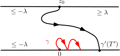
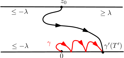
Lemma 2.6.3.
[Generalization of Lemma 2.3.8] Suppose the same the setting as in Lemma 2.6.1. Let be the level line of starting from and define to be the first time that hits . Let be the level line of starting from 0 targeted at . Then, given , almost surely, either hits the continuation threshold before hits , or hits at and merges with afterwards. See Figure 2.6.2.
Proof.
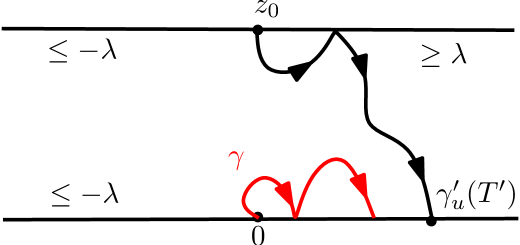
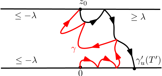
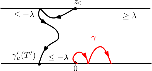
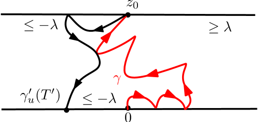
Lemma 2.6.4.
[Generalization of Proposition 2.3.11] Suppose the same the setting as in Lemma 2.6.1. Fix and let be the level line of with height starting from . Assume that does not hit its continuation threshold before reaches and define to be the first time that hits . Let be the level line of starting from 0 targeted at . See Figure 2.6.3.
-
(1)
If , then almost surely stays to the left of .
-
(2)
If , define to be the event that is to the left of 0. Then, on , the level line almost surely stays to the right of .
Proof.
Lemma 2.6.5.
[Generalization of Proposition 2.3.13] Fix . Suppose that is a on whose boundary value is piecewise constant, and is at most to the left of on . For , let be the level line of with height starting from 0 and let be the first time that accumulates in . Define to be the event that does not hit on . Then, almost surely on , lies to the left of . We emphasize that there is no restriction for the boundary data of on .
Proof.
From the proof of Proposition 2.3.13, we know that the conclusion holds if we can prove the monotonicity for one properly chosen boundary value of on . Thus it suffices to prove the monotonicity when the boundary value of is to the left of and is to the right of on where
Let be the level line of with height starting from targeted at 0. By the choice of boundary value of , we know that can neither hit nor on except at points and . Define to be the event that does not hit on . Then we have the following observations.
-
(a)
By Lemma 2.6.4, we know that, on , the path stays to the left of .
-
(b)
On , both and are non-boundary-intersecting, therefore the paths and are equal.
Combining these two facts, we obtain the conclusion. ∎
Lemma 2.6.6.
Fix two starting points . Let
be a sequence of points in . Suppose that is a on whose boundary value is on , is on , and is on for . Assume that
For , let be the level line of starting from targeted at . Then, almost surely, either or hits the continuation threshold before they hit each other, or and merge upon intersecting.
Proof.
Let be the level line of starting from and define to be the first time that hits . From Lemma 2.6.3, we have the following two observations.
-
(a)
Given , either hits its continuation threshold before hits , or hits at and merges with afterwards.
-
(b)
Given , either hits its continuation threshold before hits , or hits at and merges with afterwards.
Combining these two facts, we obtain the conclusion.∎
Lemma 2.6.7.
Fix two starting points and two heights . Let
be a sequence of points in . Suppose that is a on whose boundary value is on , is on , and is on for . Assume that
For , let be the level line of with height starting from targeted at . Then almost surely stays to the left of .
Proof.
Pick and let be the level line of with height starting from . Define to be the first time that hits . From Lemma 2.6.4, we have that stays to the left of and that stays to the right of . This implies the conclusion. ∎
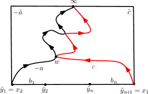
Lemma 2.6.8.
The conclusion in Lemma 2.6.7 also holds when we replace the restriction on by the following:
Proof.
Suppose that
is a sequence of points on the interval . Suppose that is a GFF on whose boundary value is on , is on , and is on for . Assume that
Set
For , let be the level line of with height starting from targeted at . For , let be the level line of with height starting from targeted at . For , define to be the event that does not hit the open interval . The restriction guarantees that has positive probability, and the restriction guarantees that has positive probability. We summarize the relations between , and as follows.
-
(a)
By Lemma 2.6.5, we know that, on , the path stays to the left of ; and that, on , the path stays to the right of .
- (b)
-
(c)
By Lemma 2.6.7, we know that stays to the left of .
Combining these three facts, given and on , we have that stays to the left of . For , define
Clearly, the event depends on the pair , and we can properly choose the sequence so that the event has positive probability. From the above analysis, we know that, given and on , the level lines of satisfy the desired monotonicity and note that the boundary value of is on , is on , and is on for where . This implies the conclusion, see Remark 2.6.9. ∎
Remark 2.6.9.
Fix two starting points and two heights . Let
be a sequence of points in . Suppose that is a on whose boundary value is on , is on , and is on for . For , let be the level line of with height starting from targeted at .
Assume that, for any , there exists a sequence
such that the following is true. Let be a on whose boundary value is on , is on , and is on for . For , let be the level line of with height starting from targeted at ; then almost surely stays to the left of .
Then we have that almost surely stays to the left of .
Proof.
For , define to be the first time of to get within distance of . We have the following observations.
-
(a)
The restriction of to is absolutely continuous with respect to the restriction of to the same domain.
-
(b)
The path stays to the left of by the assumption.
Combining these two facts, we know that almost surely stays to the left of . This holds for any , therefore almost surely stays to the left of . ∎
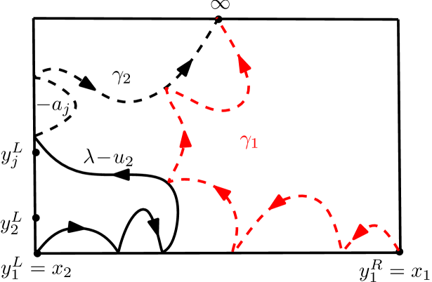
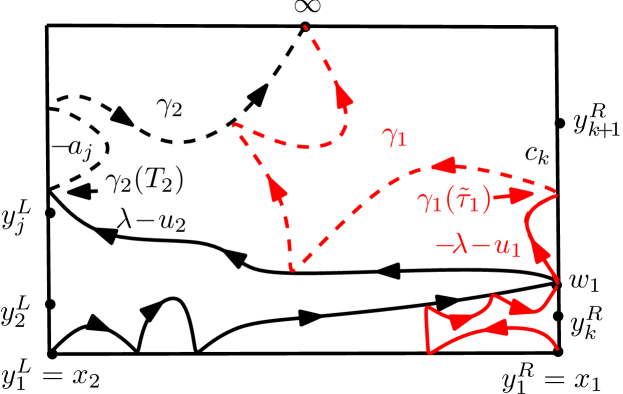
Lemma 2.6.10.
Fix two starting points and two heights . Let
be three sequences of points on the boundary of . Suppose that is a on whose boundary value is
Assume that
For , let be the level line of with height starting from targeted at . Then almost surely stays to the left of .
Proof.
We will prove the conclusion by induction on . Lemma 2.6.8 implies that the conclusion holds for . We assume that the conclusion holds for for some and we will prove that the conclusion holds for and . Define to be the first time that hits .
First, we argue that almost surely stays to the right of . For , let be the first time that gets within distance of . By induction hpothesis, we know that stays to the right of . This holds for any and we know that and are continuous, thus stays to the right of up to the first time that hits . Since is targeted at , it continues towards in the connected component of that has on the boundary. Therefore stays to the right of .
Next, we show that almost surely stays to the right of given . If is or the continuation threshold of , we are done. In the following of the proof, we assume that is finite and it is not the continuation threshold of . Suppose that . Since is not the continuation threshold, we have that . Define to be the connected component of that has on the boundary. We only need to show that stays to the right of given . There are two cases: Case 1. does not hit , see Figure 2.6.5(a); Case 2. hits , see Figure 2.6.5(b). We treat the two cases separately.
Case 1. In this case, given , the path is the level line with height starting from and the path is the level line with height starting from . By induction hypothesis (note that the conditions and guarantee that the induction hypothesis is applicable), we have that stays to the right of .
Case 2. In this case, define to be the last point of that is contained in . If hits its continuation threshold before enters , then we are done. In the following of the proof, we assume that enters , say at time . Suppose that , then . We run up to a stopping time so that and (the condition guarantees that we are able to find such a time ). Define to be the connected component of that has on the boundary. Given and , the curve is the level line of with height starting from and the curve is the level line of with height starting from . By induction hypothesis (note that the conditions and guarantee that the induction hypothesis is applicable), we know that stays to the right of given and . This completes the proof. ∎
Remark 2.6.11.
The conclusion in Lemma 2.6.10 also holds when we replace the restriction on by the following:
Proof.
The conditions on guarantee that and exist for a positive time. Pick so that exist up to time and they do not hit each other up to . We run both curves up to time . To show the conclusion, we only need to show that, given , the level line of (restricted to ) with height starting from targeted at stays to the right of the level line of (restricted to ) with height starting from targeted at . Note that, given , the field has boundary value where
This implies that we can apply Lemma 2.6.10 to show the conclusion given . ∎
Proof of Theorem 1.1.4.
Lemma 2.6.10 implies the conclusion for and . The conclusion for and can be proved by starting from Lemma 2.6.6 and then using similar proofs of Lemmas 2.6.8 and 2.6.10.
Finally, we explain the conclusion for and . Suppose that, in a small neighborhood of , the boundary value of the field is to the left of and is to the right of . In order to get the two curves and started, we must have
Take small so that and are contained in this neighborhood of . By Remark 2.4.6, we know that stays to the left of . Given , the remaining of is the level line of the field with height starting from and the remaining of is the level line of the field with height starting from . Therefore we could use the conclusion for to show the monotonicity. This completes the proof. ∎
Corollary 2.6.12.
Suppose that is a on whose boundary value is piecewise constant. Fix and two sequences of heights
satisfying
For , let be the height-varying level line of starting from targeted at with heights . Assume that
Then stays to the left of almost surely.
2.7 Proof of Theorems 1.1.6 and 1.1.7—general case
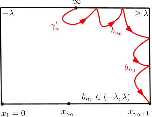
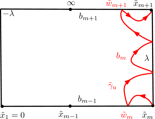
Lemma 2.7.1.
Suppose that
is a sequence of points along . Suppose that is a on whose boundary value is on and is on for . Assume that
Let be the level line of starting from 0 targeted at and let be the level line of starting from targeted at 0. Then and are equal almost surely.
Proof.
We prove by induction on . Proposition 2.5.11 implies that the conclusion holds for . Assume that the conclusion holds for for some , we will show that the conclusion holds for . If all , then Proposition 2.3.7 and Remark 2.3.9 prove the conclusion. In the following, we assume that there exists some .
First, we assume that . Define to be the number so that for and . Set . Let be the level line of with height starting from targeted at . See Figure 2.7.1(a). We summarize the relations between and as follows.
-
(a)
By Theorem 1.1.4, the path stays to the left of .
-
(b)
By Lemma 2.6.4, the path stays to the left of .
-
(c)
Define to be the connected component of that has on the boundary, and let be any conformal map from onto that sends to and to . Given , the law of is the same as a GFF on whose boundary value is on , is greater than on , and changes at most times on .
Combining these three facts with the induction hypothesis, we know that, given , the paths and are equal which implies that and are equal.
From the first step and symmetry, we know that the conclusion also holds for . In the following we assume that and .
Second, we assume that there exists some such that . For any define to be the open set obtained by removing from all points that are within distance of . Define to be the event that the distance between and is at least . Let be a GFF on whose boundary value is consistent with except on and is on . Let be the level line of starting from 0 targeted at and let be the level line of starting from targeted at 0. Then we have the following facts.
-
(a)
By the induction hypothesis, we have that and are equal.
-
(b)
The law of restricted to is absolutely continuous with respect to the law of restricted .
Combining these two facts, we know that, on , the curves and are equal. Since that the boundary value on is at least , the union has positive distance from almost surely. Therefore as , this implies the conclusion.
Finally, we assume that for all . Suppose that
is a sequence of points on . Suppose that is a GFF on whose boundary value is on , is on for except for , and is on . Let be the level line of starting from 0 targeted at and be the level line of starting from targeted at . Set , and let be the level line of with height starting from targeted at . See Figure 2.7.1(b). We summarize the relations between and in the following.
-
(a)
By the second step, we have that and are equal.
-
(b)
By Theorem 1.1.4, we have that stays to the left of .
-
(c)
Define to be the event that reaches before hits the continuation threshold and does not hit the union . The conditions
guarantee that has positive probability. On , let be the connected component of that has on the boundary and let by any conformal map from onto that fixes and . On , define to be the last point of that is contained in and to be the first point of that is contained in .
Combining these three facts, we have that, given and on , the paths and are equal. For , define
Clearly, the event depends on , and we can properly choose the sequence so that the event has positive probability. From the above analysis, we know that, given and on , the level line of starting from 0 targeted at coincides with the level line of starting from targeted at 0. Note that, on , the boundary value of is on , and is on for , is on , is on , and is on . This implies the conclusion, see Remark 2.7.2. ∎
Remark 2.7.2.
Suppose that
is a sequence of points along . Suppose that is a on whose boundary value is on and is on for where for . Let be the level line of starting from 0 targeted at and let be the level line of starting from targeted at 0.
Assume that, for any , there exists a sequence
such that the following is true. Let be a on whose boundary value is on and is on for . Let be the level line of starting from 0 targeted at and let be the level line of starting from targeted at 0, then and are equal almost surely.
Then and are equal almost surely.
Proof.
Define (resp. ) to be the event that the distance between (resp. ) and is at least . We have the following observations.
-
(a)
The restriction of to is absolutely continuous with respect to the restriction of to the same domain.
-
(b)
The paths and are equal by the assumption.
Combining these two facts, we know that, on the event , the paths and are equal. This holds for any . Note that, since , the points are not continuation thresholds for and . Therefore, the distance between and is almost surely positive. This implies the conclusion. ∎
Remark 2.7.3.
The conclusion in Lemma 2.7.1 holds more generally when the boundary value of is piecewise constant, and is at most on .
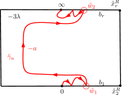
Lemma 2.7.4.
The conclusion in Lemma 2.7.1 also holds when we replace the restriction on by the following: .
Proof.
We may assume that . Suppose that
is a sequence of points on . Suppose that is a GFF on whose boundary value is on , is on for . Let be the level line of starting from 0 targeted at and be the level line of starting from targeted at . Set , and let be the level line of with height starting from targeted at . See Figure 2.7.2. We summarize the relations between and in the following.
-
(a)
By Lemma 2.7.1, we have that and are equal.
-
(b)
By Theorem 1.1.4, we have that stays to the left of .
-
(c)
Define to be the event that does not hit the interval . The conditions
guarantee that has positive probability. On , define to be the connected component of that has on the boundary, define to be the last point of that is contained in and to be the first point of that is contained in , and let be any conformal map from onto that sends to and to .
Combining these three facts, we have that, given and on , the paths and are equal. For , define
Clearly, the event depends on , and we can properly choose the sequence so that the event has positive probability. From the above analysis, we know that, given and on , the level line of starting from 0 targeted at coincides with the level line of starting from targeted at 0. Note that, on , the boundary value of is on , and is on for where . By a similar analysis as in Remark 2.7.2, we obtain the conclusion.∎
Proposition 2.7.5.
Suppose that
are two sequences of points along . Suppose that is a on whose boundary value is
Assume that
Let be the level line of starting from 0 targeted at and be the level line of starting from targeted at . Then and are equal almost surely.
By Lemma 2.7.4, we know that the conclusion in Proposition 2.7.5 holds for . Before we prove Proposition 2.7.5, we first prove that the conclusion holds for and .
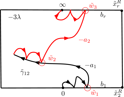
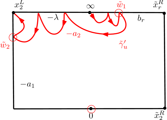
Lemma 2.7.6.
The conclusion in Proposition 2.7.5 holds when .
Proof.
If and , the conclusion holds by Remark 2.7.3. In the following, we assume that .
First, we assume that and . Suppose that
is a sequence of points along . Suppose that is a GFF on whose boundary value is on , is on for . Let be the level line of starting from 0 targeted at and be the level line of starting from targeted at 0. Set
Let be the height-varying level line of starting from 0 targeted at with heights and height change time . We summarize the relations between , , and in the following. See Figure 2.7.3(a).
-
(a)
By Lemma 2.7.1, we know that and are equal.
-
(b)
By Corollary 2.6.12, we know that stays to the left of .
-
(c)
Define to be the event that does not hit the interval and that does not hit the interval . The conditions
guarantee that has positive probability. On , define to be the last point of that is contained in ; define to be the last point of that is contained in if and to be if ; define to be the first point of that is contained in . On , define to be the connected component of that has on the boundary, and define to be the conformal map from onto that sends to 0, to , and to .
Combining these three facts, we know that, given and on , the paths and are equal. For , define
We can properly choose the sequence so that has positive probability. From the above analysis, we know that, given and on , the level line of starting from 0 targeted at coincides with the level line of starting from targeted at 0. Note that, on , the boundary value of is on , is on , is on for where . By a similar analysis as in Remark 2.7.2, we obtain the conclusion.
Next, we assume that and . Suppose that
is a sequence of points along . Suppose that is a GFF on whose boundary value is on , is on , and is on for . Let be the level line of starting from 0 targeted at and be the level line of starting from targeted at 0. Set
Let be the level line of with height starting from targeted at . We summarize the relations between , , and in the following. See Figure 2.7.3(b).
-
(a)
By Remark 2.7.3, we know that and are equal.
-
(b)
By Theorem 1.1.4, we know that stays to the left of .
-
(c)
Define to be the event that reaches before hits its continuation threshold and that does not hit the interval . The conditions
guarantee that has positive probability. On , define to be the connected component of that has on the boundary, define to be the last point of that is contained in and to be the first point of that is contained in , and let be the conformal map from onto that sends to , to , and to .
Combining these three facts, we know that, given and on , the paths and are equal. For , define
We can properly choose the sequence so that has positive probability. From the above analysis, we know that, given and on , the level line of starting from 0 targeted at coincides with the level line of starting from targeted at 0. Note that, on , the boundary value of is on , is on , is on for where . By a similar analysis as in Remark 2.7.2, we obtain the conclusion. ∎
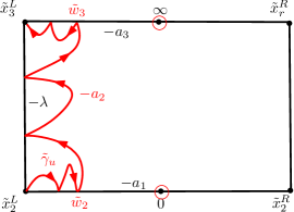
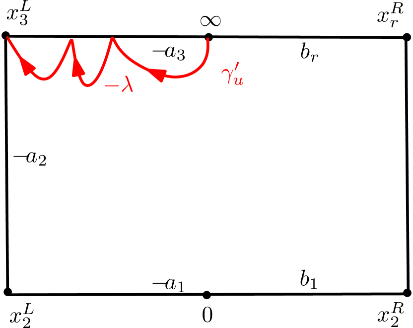
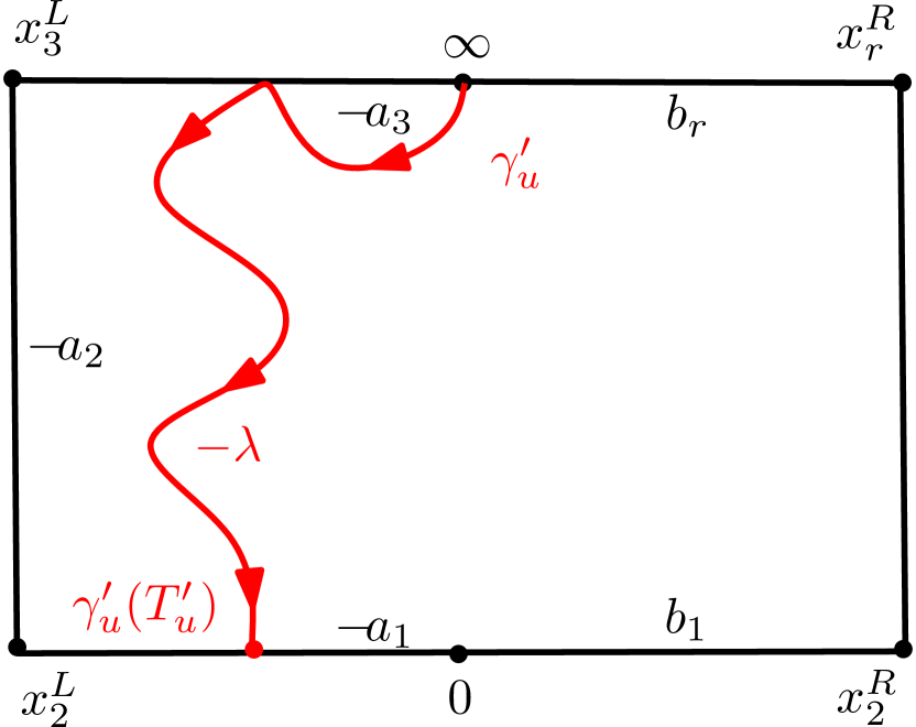
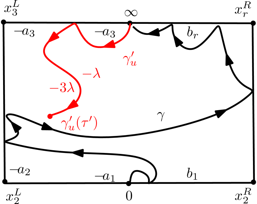
Lemma 2.7.7.
The conclusion in Proposition 2.7.5 holds when .
Proof.
We divide the proof into three cases according to the boundary value: Case 1. ; Case 2. ; Case 3. and . We treat these three cases separately.
Case 1. We assume that . By a similar proof as the second step in the proof of Lemma 2.7.1, we have that the conclusion holds by Lemma 2.7.6.
Case 2. We assume that and . Suppose that
are two sequences of points along . Suppose that is a GFF on whose boundary value is
and is
Let be the level line of starting from 0 targeted at and be the level line of starting from targeted at 0. Set
Let be the level line of with height starting from targeted at . See Figure 2.7.4. We summarize the relations between , , and in the following.
-
(a)
By Case 1, we have that and are equal.
-
(b)
By Theorem 1.1.4, we have that stays to the right of .
-
(c)
Define to be the event that reaches before hits the continuation threshold and that does not hit the union of the intervals . The conditions
guarantee that has positive probability. On , define to be the connected component of that has on the boundary, define to be the last point of that is contained in and to be the first point of that is contained in , and let be any conformal map from onto that sends to , to .
Combining these three facts, we know that, given and on , the paths and are equal. For , define
We can properly choose the sequences so that has positive probability. From the above analysis, we know that, given and on , the level line of starting from 0 targeted at coincides with the level line of starting from targeted at 0. Note that, on , the boundary value of is on , is on , is on , and is on for where , and . By a similar analysis as in Remark 2.7.2, we obtain the conclusion.
Case 3. We assume that . Set and let be the level line of with height starting from targeted at .
First, we analyze the behavior of . The conditions
guarantee the existence of . The conditions
guarantee that can not hit the union . There are two possibilities: either reaches without hitting , see Figure 2.7.5(a); or hits , see Figure 2.7.5(b). In the former case, define to be ; and in the latter case, define to be the first time that hits .
Second, we argue that stays to the left of . Suppose that is any -stopping time such that . Given , the conditional law of is the same as the level line of restricted to whose boundary value is as depicted in Figure 2.7.5(c). Therefore, given , the path can not hit the union . This implies that stays to the left of . This holds for any . By the continuity of and , we know that stays to the left of .
Finally, we show that and are equal. We summarize the relation between and as follows.
-
(a)
By Theorem 1.1.4, we have that stays to the right of .
-
(b)
By the above analysis, we have that stays to the right of .
-
(c)
Define to be the connected component of that has on the boundary. Given , the boundary value of is as depicted in Figure 2.7.5(a) and (b).
Combining these three facts, given , in the case that does not hit (Figure 2.7.5(a)), the paths and are equal by Case 2.; in the case that hits (Figure 2.7.5(b)), the paths and are equal by Lemma 2.7.6. This completes the proof. ∎
Proof of Proposition 2.7.5.
We will prove by induction on . Lemmas 2.7.4, 2.7.6 and 2.7.7 imply that the conclusion holds for . Assume that the conclusion holds for for some , we will show that the conclusion holds for .
First, we assume that there exists some such that . By a similar proof as the second step in the proof of Lemma 2.7.1, we have that the conclusion holds by induction hypothesis.
Second, we assume that there exists such that
By a similar proof of Case 2 in the proof of Lemma 2.7.7, we have that the conclusion holds.
Finally, we point out that, if we are not in the case of the first step, then we have that which implies that , therefore we are in the case of the second step. Thus, the above two steps address all cases and complete the proof. ∎
Proof of Theorem 1.1.7.
First, we assume that the boundary value of is at most on , is at least on , and is in on . For , let be the level line of starting from targeted at . We summarize the relations between and in the following.
-
(a)
By Lemma 2.7.1, we have that and are equal and that and are equal.
-
(b)
By Lemma 2.6.3, we have that, given , the path first hits at and merges with afterwards.
Combining these two facts, we obtain the conclusion.
3 The coupling between and with time parameter
3.1 Radial
The radial Loewner equation describes the evolution of hulls growing from the boundary of the unit disc towards the origin. Suppose that is a continuous function from to . For each , define the function to be the solution to Radial Loewner Equation
This is well-defined as long as does not hit . Define
This is the largest time up to which is well-defined. Set
Then is the unique conformal map from onto such that and . In fact, . In other words, the time is parameterized by minus the log conformal radius of seen from the origin.
The family is called the radial Loewner chain driven by . Radial for is the radial Loewner chain driven by where is one-dimensional Brownian motion.
Proposition 3.1.1.
For all , radial is almost surely generated by a simple continuous curve , i.e. there exists a simple continuous curve such that for all .
Proof.
[LSW01, Proposition 4.2]. ∎
Define
| (3.1.1) |
Suppose , , and . Radial with force point is the Loewner chain driven by which is the solution to the following SDE:
| (3.1.2) |
where
| (3.1.3) |
Note that the processes and take values in . We say that the process describes the radial process with force point and weight .
We first explain the existence of the solution to Equation (3.1.2) for . Set , and assume that , then satisfies the SDE:
| (3.1.4) |
The process is well defined up to . Note that, as , we have . Hence, when is close to 0, the evolution of is absolutely continuous with respect to times a Bessel process of dimension . Similarly, when is close to , the process is absolutely continuous with respect to times a Bessel process of the same dimension.
Note that
Thus the existence and uniqueness of the solution to Equation (3.1.4) guarantees the existence and uniqueness of the solution to Equation (3.1.2).
Next we explain the geometric meaning of the process : is the image of the tip of under . For , there are two different cases: if , then is the image of under ; if , then is the image of the last point on the boundary that hits by time under . See Figure 3.1.1.
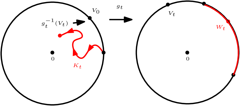
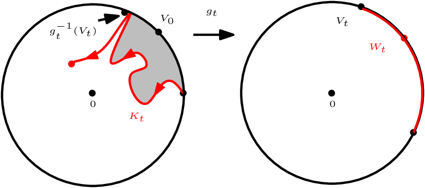
The relation between radial for different ’s is as follows: Suppose that , , , . Let be the radial Loewner chain corresponding to the radial process with force point , and be the corresponding family of conformal maps. Define
Then is well-defined up to the first time collides with , and is a local martingale. The law of weighted by is the same as that of a radial process with force point as long as one stops at a bounded stopping time that occurs before gets within some fixed distance of .
One can also consider the radial with two boundary force points .
Definition 3.1.2.
Fix , , and three boundary points which are located on in counterclockwise order. Let be a standard Brownian motion. We will say that the process describes a radial process with force points if they are adapted to the filtration of and the following hold:
- (1)
-
(2)
We have instantaneous reflection of off of the and .
-
(3)
We also have almost surely that
Define the continuation threshold for the process :
-
•
if , the continuation threshold is the infimum of for which ;
-
•
if , the continuation threshold is the infimum of for which ;
-
•
if , the continuation threshold is the infimum of for which either or ;
-
•
if , , the continuation threshold is the infimum of for which ;
-
•
if , the continuation threshold is never reached.
Lemma 3.1.3.
In the setting of Definition 3.1.2, the joint law of is uniquely determined up to the continuation threshold. Under this law, is a continuous multidimensional Markovian process indexed by .
Proof.
This can be proved by a similar proof as the proof of Proposition 2.1.5. ∎
There is a close relation between radial and chordal . To describe this relation, we need to introduce chordal with interior force point. We will not address the most general case, we only introduce the process that we will use in the current paper: chordal with two boundary force points and one interior force point.
Definition 3.1.4.
Fix , , and , . Chordal with force points is the chordal Loewner chain driven by which is the solution to the following SDE:
We can define chordal in the unit disc via conformal transformations. Fix four boundary points along which are located in counterclockwise order. Define to be the conformal map from onto such that . Define chordal in starting from targeted at with force points to be the image of chordal in with force points under the conformal map . Chordal with interior force point and radial SLE are closely related.
Lemma 3.1.5.
Fix , . Fix four boundary points along which are located in counterclockwise order. Let be the chordal process in starting from targeted at with force points . Define to be the first time that and the origin are disconnected by . Let be the radial starting from with force points . Define be the first time that and the origin are disconnected by . Assume that
Then the path stopped at has the same law as the path stopped at (up to time change).
3.2 Conformal Loop Ensemble
3.2.1 Carathéodory topology
We say that a sequence of functions on a domain converges to uniformly on compact sets if, for any compact , the functions converge to uniformly on .
Suppose that is a sequence of simply connected domains other than containing the origin, and let be the conformal map from onto such that . We define convergence in Carathéodory topology as follows:
-
(1)
converges to if .
-
(2)
converges to if .
-
(3)
converges to (which is simply connected other than ) if converges to uniformly on compact sets where is the conformal transformation from onto such that .
If is a sequence of simply connected domains other than containing some fixed . We say that converges to in Carathéodory topology seen from if converges to in the above sense.
Lemma 3.2.1.
Suppose that and are simply connected domains other than containing the origin. Assume that is decreasing:
and that
Then converges to in Carathéodory topology if and only if the sequence of conformal radius converges to .
Proof.
We only need to show that the convergence in conformal radii implies the convergence in Carathéodory topology. Let be the conformal map from onto such that , and be the conformal map from onto such that .
From [Law05, Proposition 3.61], we know that there exist a conformal map from onto some and a subsequence such that converges to uniformly on compact sets. Therefore, the sequence converges to in Carathéodory topology. Furthermore . We have the following observations.
-
(a)
Since for all , we have that .
-
(b)
Since as , we have that .
Combining these two facts, we have that . Therefore, converges to in Carathéodory topology. Since the sequence is decreasing, we have that converges to in Carathéodory topology. ∎
3.2.2 and the exploration process
In this section, we recall some features of CLE and we refer to [SW12] for details and proofs of the statements. CLE in is a collection of non-nested disjoint simple loops in that possesses the following two properties.
-
(1)
[Conformal Invariance] For any Möbius transformation of onto itself, the laws of and are the same. This makes it possible to define, for any non-trivial simply connected domain (that can therefore be viewed as the conformal image of via some map ), the law of CLE in as the distribution of (because this distribution does not depend on the actual choice of conformal map from onto ).
-
(2)
[Domain Markov Property] For any non-trivial simply connected domain , define the set obtained by removing from all the loops (and their interiors) of that do not entirely lie in . Then, conditionally on , and for each connected component of , the law of those loops of that do stay in is exactly that of a CLE in .
The loops in CLE are -type loops for some . In fact, for each such value of , there exists exactly one CLE distribution that has -type loops. We denote the corresponding CLE by for .
We call a bubble in if is homeomorphic to the unit circle and contains exactly one point; we call the point in the root of , denoted by .
In [SW12], the authors introduce a discrete exploration process of CLE loop configuration. The conformal invariance and the domain Markov property make the discrete exploration easy to control. Consider a CLE in , draw a small disc with center , let be the loop that intersects with largest radius. Define the quantity
In fact, as goes to zero where .
Lemma 3.2.2.
The law of normalized by converges towards a limit measure, denoted by .
Proof.
[SW12, Section 4]. ∎
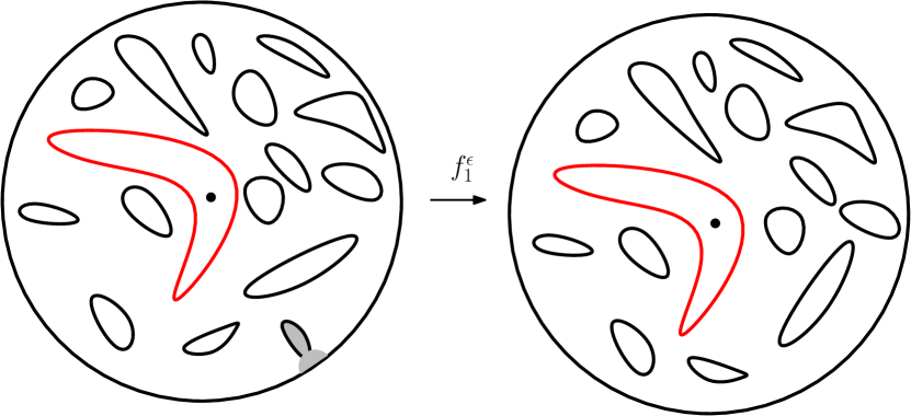
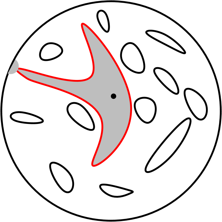
Because of the conformal invariance and the domain Markov property, we can repeat the “small semi-disc exploration” until we discover the loop containing the origin: Suppose we have a CLE loop configuration in the unit disc . We draw a small semi-disc of radius whose center is uniformly chosen on the unit circle. The loops that intersect this small semi-disc are the loops discovered. If we do not discover the loop surrounding the origin, we refer to the connected component of the remaining domain that contains the origin as the to-be-explored domain. Let be the conformal map from the to-be-explored domain onto such that . We also define to be the loop discovered with largest radius. Because of the conformal invariance and the domain Markov property of CLE, the image of the loops in the to-be-explored domain under the conformal map has the same law as simple CLE in the unit disc. Thus we can repeat the same procedure for the image of the loops under . We draw a small semi-disc of radius whose center is uniformly chosen on the unit circle. The loops that intersect the small semi-disc are the loops discovered at the second step. If we do not discover the loop surrounding the origin, define the conformal map from the to-be-explored domain onto such that . The image of the loops in the to-be-explored domain under has the same law as CLE in the unit disc, etc. At some finite step , we discover the loop surrounding the origin, we define to be the loop surrounding the origin discovered at this step and stop the exploration. We summarize the properties and notations in this discrete exploration below. See Figure 3.2.1.
-
(a)
Before , all steps of discrete exploration are i.i.d.
-
(b)
The number of the step , when we discover the loop surrounding the origin, has the geometric distribution:
-
(c)
Define the conformal map
As goes to zero, the discrete exploration will converge to a Poisson point process of bubbles with intensity measure given by
where is Lebesgue length measure on .
Now we can reconstruct CLE loops from the Poisson point process of SLE bubbles. Let be a Poisson point process with intensity . Namely, let be a Poisson point process with intensity , and then arrange the bubble according to the time , i.e. denote as the bubble if , and is empty set if there is no that equals . Clearly, there are only countably many bubbles in that are not empty set. Define
For each , the bubble does not surround the origin. Define to be the conformal map from the connected component of containing the origin onto the unit disc such that . For this Poisson point process, we have the following properties:
-
(a)
has the exponential law: .
-
(b)
For small, let be the times before at which the bubble has radius greater than . Define . Then almost surely converges towards some conformal map in Carathéodory topology seen from the origin as goes to zero. Therefore can be interpreted as .
-
(c)
Generally, for each , we can define . Then
is a collection of loops in the unit disc and is a loop surrounding the origin.
The relation between this Poisson point process of bubbles and the discrete exploration process we described above is given via the following result.
Proposition 3.2.3.
converges in distribution to in Carathéodory topology seen from the origin. Moreover, the loop has the same law as the loop of in that surrounds the origin.
Proof.
[SW12, Section 7]. ∎
The results in this section hold for all . In the next section, we will point out a particular property that only holds for .
3.2.3 with time parameter
In this section, we will introduce with time parameter. We refer to [WW13] for the details and proofs of the statements. Throughout this section, we fix . Recall that is the SLE bubble measure rooted at defined in Lemma 3.2.2, and is defined by
The following property only holds for and it is the most important ingredient in the construction of with time parameter.
Lemma 3.2.4.
When , the bubble measure is conformally invariant: for any Möbius transformation of , we have
Proof.
[WW13, Lemma 6]. ∎
We call the bubble measure uniformly rooted over the boundary. Let be a Poisson point process with intensity . The sequence of loops is obtained from by targeting at the origin described in Section 3.2.2. In fact, we can construct a sequence of loops from by targeting at any interior point . Given , define
For each , let be the conformal map from the connected component of that contains onto such that . For each , define . Then
is a collection of loops in the unit disc and has the same law as the loop in CLE that surrounds .
The conformal invariance in leads to the following “target-independent property”. Suppose that we have two distinct target points , the process and the process , up to the first time that and are disconnected, have the same law [WW13, Lemma 8]. Therefore, we can couple the two processes in the following way: up to the first time that and are disconnected, the two processes of loops coincide; and after the disconnecting time, the two processes evolve independently towards their target points respectively. Consequently, it is possible to couple for all simultaneously in the way that, for any two points , the previous statement holds. This is the conformal invariant growing mechanism in constructed in [WW13]. From this growing process, we obtain a collection of loops and, moreover, each loop has a time parameter: . We call with time parameter. It satisfies conformal invariance in the following sense.
Proposition 3.2.5.
For , let be the domain obtained by removing from all the loops with . Then, for any Möbius transformation of , the process has the same law as the process .
Proof.
[WW13, Proposition 9]. ∎
3.3 Level lines targeted at interior points
In Section 2, we studied the level line of GFF starting from a boundary point and targeted at a distinct boundary point. In this section, we will study the level line of GFF starting from a boundary point and targeted at an interior point.
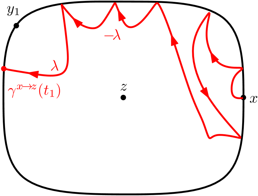
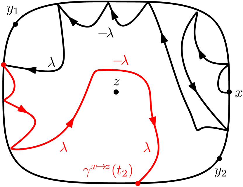
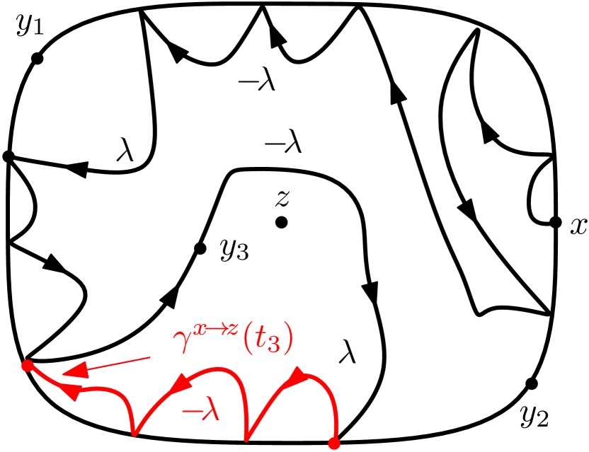
Suppose that is a GFF on whose boundary value is piecewise constant. Fix a boundary point and an interior point . We define the level line of starting from targeted at , denoted by , in the following way. See Figure 3.3.1.
Pick a point different from . We start by the level line of starting from targeted at . We parameterize the curve by minus the log of the conformal radius of seen from . Namely, the curve is parameterized so that
Define to be the first disconnecting time: the first time that is not on the boundary of the connected component of that contains . Denote by the connected component of that contains . Generally, when and are defined for some , we pick on the boundary of different from . Given , we continue the curve by the level line of restricted to starting from targeted at and parameterize the curve by minus the log of the conformal radius seen from . Define to be the first disconnecting time: the first time that is not on the boundary of the connected component of that contains . Denote by the connected component of that contains . We continue this procedure until the curve hits the continuation threshold . We summarize some basic properties of in the following.
-
(a)
The curve is parameterized by minus the log of the conformal radius:
-
(b)
By the target-independent property of the level lines in Theorem 1.1.7, we have that the curve is independent of the choice of the sequence .
-
(c)
The curve is almost surely determined by the field and is almost surely continuous up to and including the continuation threshold.
Generally, for , the level line of with height starting from targeted at , denoted by , is the level line of starting from targeted at .

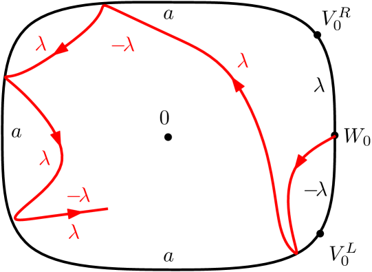
By Lemma 3.1.5, the level line targeted at interior point is radial process and we record this fact in the following proposition.
Proposition 3.3.1.
Fix and three boundary points that are located on in counterclockwise order. Suppose that is a on whose boundary value is on , is on , and is on (the intervals are counterclockwise). See Figure 3.3.2(a).
Suppose that is a radial process starting from with two force points and the corresponding weights
Note that the continuation threshold of is hit at the following time
which is almost surely finite.
There exists a coupling between and so that the following is true. Suppose that is any -stopping time less than the continuation threshold for . Then, given , the conditional law of restricted to is in each connected component whose boundary value is consistent with on and is to the right of and is to the left of . See Figure 3.3.2(b).
Furthermore, in this coupling, the path is almost surely determined by and is continuous up to and including the continuation threshold.
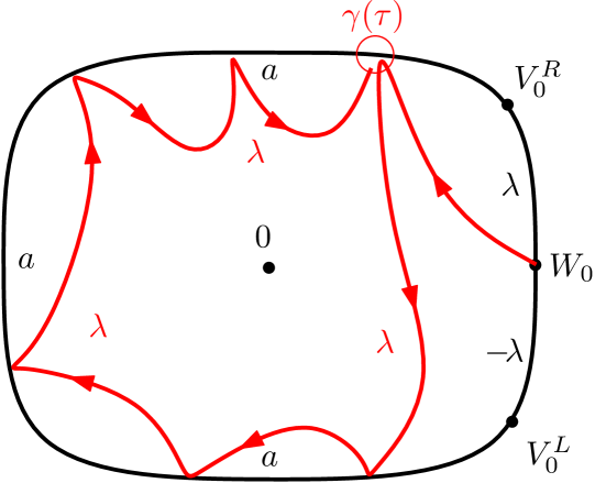
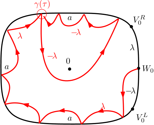
Corollary 3.3.2.
Proof.
For small, recall that the average of in , denoted by , is defined through Equation (LABEL:eqn::gff_localmean). We have the following.
-
(a)
The variable is a Gaussian with mean and variance .
-
(b)
Given and on the event , the variable is a Gaussian with mean and variance (recall that is minus the log of the conformal radius of ).
Combining these two facts and letting go to zero, we have that
This implies the conclusion. ∎
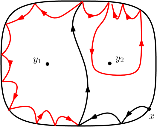
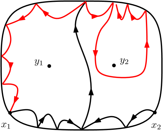
By the construction of the level lines targeted at interior points, we have that these level lines also satisfy target-independent property.
Proposition 3.3.3.
[Generalization of Theorem 1.1.7] Suppose that is a on whose boundary value is piecewise constant. Fix three points and . For , let be the level line of starting from targeted at ; define to be the first disconnecting time: is the inf of time such that are not in the same connected component of . See Figure 3.3.4(a). Then, almost surely, the paths and coincide up to and including the first disconnecting time (up to time change); given , the two paths continue towards their target points independently.
Furthermore, the same conclusion holds when one or two of the target points are on the boundary.
Remark 3.3.4.
A similar conclusion as in Proposition 3.3.3 also holds when the two starting points are distinct. Suppose that is a on whose boundary value is piecewise constant. Fix two distinct starting points and two distinct target points . For , let be the level line of starting from targeted at . On the event that the two paths hit each other, the two paths will merge upon intersecting, continue together until the first disconnecting time after which the two paths continue towards their own target points independently. See Figure 3.3.4(b).
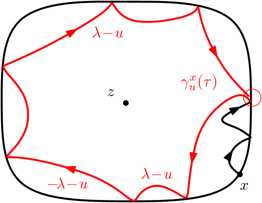
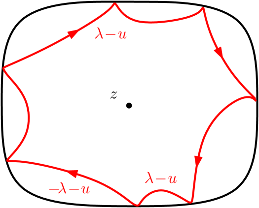
Suppose that is a zero-boundary GFF on . Fix a height and a target point . Let be the level line of with height starting from targeted at , and define to be its continuation threshold. Let be the connected component of that contains , and let be the oriented boundary of . By Remark 3.3.4, we know that is independent of the starting point . In other words, the level line depends on but does not. We call the level loop of starting from the boundary targeted at . We denote by the connected component of that contains . We record some basic properties of the level loop in the following lemma.
Lemma 3.3.5.
Suppose that is a zero-boundary on . Fix a height and a target point . Let be the level loop of starting from the boundary targeted at . Then we have the following.
-
(1)
is oriented either clockwise or counterclockwise and is homeomorphic to the unit disc.
-
(2)
.
-
(3)
Given , the conditional law of restricted to each connected component of is the same as ’s whose boundary value is zero on , is to the right of , and is to the left of . See Figure 3.3.5. In particular, the conditional law of restricted to is the same as a whose boundary value is
Moreover, the loop is almost surely determined by and
In fact, the three properties in Lemma 3.3.5 characterize the level loop of .
Lemma 3.3.6.
Suppose that is a zero-boundary on . Fix a height and a target point . Let be the level loop of starting from the boundary targeted at . Assume that is an oriented loop in satisfying the three properties in Lemma 3.3.5. Then almost surely and are equal.
Proof.
For , let be the level line of with height starting from targeted at . We have the following observations.
-
(a)
On the event that hits , the level line will merge with (since satisfies the third property in Lemma 3.3.5) upon intersecting; therefore, and are equal.
-
(b)
.
Combining these two facts, we obtain the conclusion. ∎

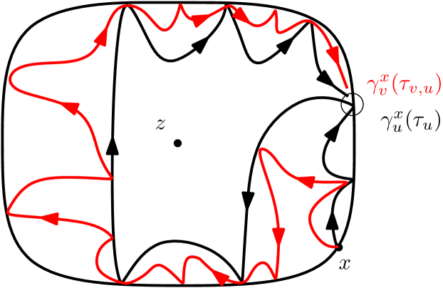
The following proposition addresses the interaction between two level loops.
Proposition 3.3.7.
Suppose that is a zero-boundary on . Fix a target point . For , denote by the level loop of with height starting from the boundary targeted at . Fix .
If is clockwise, then, for any , the loop is outside of and is also clockwise. Moreover, given , the conditional law of is the same as the level loop of a zero-boundary on with height starting from the boundary targeted at , conditioned on the event that the loop is clockwise.
If is counterclockwise, then, for any , the loop is outside of and is also counterclockwise. Moreover, given , the conditional law of is the same as the level loop of a zero-boundary on with height starting from the boundary targeted at , conditioned on the event that the loop is counterclockwise.
Proof.
We only need to prove the conclusion when is clockwise. Let (resp. ) be the level line of with height (resp. height ) starting from targeted at and (resp. ) be its continuation threshold. By the construction of level lines targeted at interior point and Theorem 1.1.4, we know that stays to the left of until the time that reaches , say at time . See Figure 3.3.6. This implies that is outside of . This holds for any and we know that is independent of , thus is outside of . ∎
Suppose that is a zero-boundary GFF on and . Fix a target point . Let be the level loop of with height starting from the boundary targeted at . The rest of this section is devoted to the study of the asymptotic behavior of the level loop as .
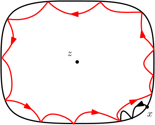
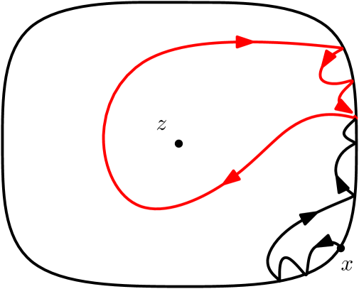
There are two possibilities for the orientation of : counterclockwise (with probability ) or clockwise (with probability ). Lemma 3.3.8 addresses the first case: when is counterclockwise, the loop will converge to as . See Figure 3.3.7(a). Lemma 3.3.9 addresses the second case: when (conditioned on) is clockwise, the loop will converge to some bubble as . See Figure 3.3.7(b).
Lemma 3.3.8.
Suppose that is a zero-boundary on . Fix a target point . Let be the level loop of with height starting from the boundary targeted at . Then, almost surely,
Moreover, there exists a universal constant such that
| (3.3.1) |
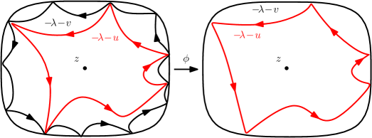
Proof.
First, we show that is almost surely monotone as . For , suppose that is counterclockwise. By Proposition 3.3.7, we know that, for , the loops and are counterclockwise and that is outside of . Therefore,
Thus, on the event , the sequence is monotone. Note that the event has probability . Letting , we obtain the conclusion.
Second, we have the following observations.
-
(a)
The sequence is almost surely monotone as .
-
(b)
The sequence converges to 1 in distribution as .
Combining these two facts, we have that, almost surely, as .
Finally, we show Equation (3.3.1). For , suppose that is counterclockwise. Then, for , the loop is counterclockwise; define
Let be small and set , . We have the following observations.
-
(a)
The loops are counterclockwise and is outside of . Define to be the conformal map from onto such that . Then
-
(b)
Given , the loop has the same law as the level loop of zero-boundary GFF in with height . See Figure 3.3.8. Thus
Combining these two facts, we have that
where is a copy of and is independent of . Therefore, there exists a universal constant such that
∎
Lemma 3.3.9.
Suppose that is a zero-boundary on . Fix a target point . Let be the level loop of with height starting from the boundary targeted at . Denote by the law of conditioned on the event . Then, as , the measure converges to some limit measure, denoted by , in Carathéodory topology seen from .
Moreover, the limit measure is conformal invariant: for any Möbius transformation of , we have that
Proof.
For , on the event , we know that is also clockwise and that is inside of . By Lemma 3.2.1, to show the convergence in Carathéodory topology, we only need to show the convergence in .
Suppose that is any bounded Lipschitz function.
Given and , the conditional law of is the same as the level loop of a zero-boundary GFF with height . Define to be the conformal map from onto such that . Then we have that
This implies the convergence.
The conformal invariance in the limit measure is inherited from the conformal invariance in the level loops: for any Möbius transformation of , the loop has the same law as the level loop with height targeted at . ∎
We give some properties of the limit measure defined in Lemma 3.3.9. Recall that is a bubble in if is homeomorphic to the unit circle and contains exactly one point; and the point in is called the root of , denoted by . The (probability) measure is supported on clockwise bubbles in . For any , let be a bubble with law . By the conformal invariance in , we know that, for any Möbius transformation , we have
In particular, the root is uniform over .
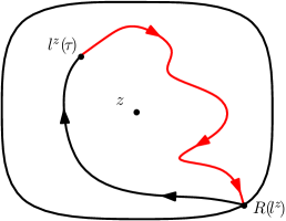
The measure inherits the “domain Markov property” from the level loop in the following sense. Suppose that is a bubble with law . We parameterize clockwise by minus the log of the conformal radius seen from :
Then the bubble satisfies the following property. For any stopping time , given , the conditional law of is the same as chordal (up to time change) in from to conditioned on the event that is to the right of the path. See Figure 3.3.9.
We can define an infinite measure on bubbles: it is the measure on bubbles such that, for any , it coincides with on the set of bubbles that surround .
First, we explain that is well-defined. For any two points , we need to show that the two measures and coincide on the set of bubbles that surround both and . To this end, we only need to show that, for any , the two measures and coincide on the set of loops that surround both and . Suppose that is a zero-boundary GFF on and that (resp. ) is the level loop of with height starting from the boundary targeted at (resp. targeted at ). Then, when restricted to the set of loops that surround both and , we have that
This implies that and coincide on the set of loops that surround both and .
Furthermore, the requirement that coincides with the ’s full determines . Thus is well-defined.
Next, we explain that is the same as the measure of bubble measure defined in Section 3.2.3. We record this in the following lemma.
Lemma 3.3.10.
The infinite measure equals , bubble measure (oriented to be clockwise) uniformly rooted over the boundary.
Proof.
By the conformal invariance of , we also have the conformal invariance of : for any Möbius transformation of , we have that
To show that equals , we only need to show that , which is restricted to the bubbles that surround the origin, equals , which is restricted to the bubbles that surround the origin. In fact, the domain Markov property of characterizes the bubble measure [SW12, Section 6]. Therefore is a multiple of . Since the total mass of is 1 and the total mass of is also 1, we have that equals . ∎
3.4 Upward height-varying level lines
We will introduce height-varying level lines targeted at interior points. We do not plan to address the general case, we only focus on one particular type of height-varying level lines: upward height-varying level lines. Suppose that is a zero-boundary on . Fix , a boundary point and a target point . We define the upward height-varying level line of starting from targeted at with height difference , denoted by or , in the following way.
For , set
We start by the level line of with height starting from targeted at , and define to be its continuation threshold. Let be the connected component of that contains . By Corollary 3.3.2, we know that, given , the conditional mean of restricted to is either or ; moreover,
By Proposition 3.3.1, we know that the law of is the same as radial . Denote by the corresponding radial Loewner evolution. Note that
Assume , then, as , we have that
If , we stop and set , . If , we continue.
Generally, given and for some , we continue by the level line with height starting from targeted at , and define to be its continuation threshold. Let be the connected component of that contains . Given , the conditional mean of restricted to is either (with chance ) or (with chance ). Denote by the corresponding radial Loewner evolution. Note that
Assume , then, as , we have that
If , we stop and set and . If , we continue.
At each step, we have chance to stop. Therefore, we will stop at some finite step almost surely. When we stop, we have and
Moreover, when , we have that
This path is called the upward height-varying level line of with height difference starting from targeted at . We call the transition step and the transition time. We summarize some basic properties of in the following.
-
(a)
The path is parameterized by minus the log of the conformal radius:
-
(b)
The path is almost surely determined by and is almost surely continuous up to and including the transition time.
-
(c)
The transition step satisfies geometric distribution:
-
(d)
Suppose that is the sequence of height change times and that is the corresponding Loewner evolution. Then, for , the process satisfies the SDE for radial .
Suppose that is a zero-boundary GFF. Fix and a target point . Let be the upward height-varying level line of with height difference starting from some targeted at . Let be the transition step, be the transition time, and be the sequence of height change times. Let be the level loop of with height starting from targeted at . We know that is part of . Denote by the connected component of that contains . Generally, given for some , let be the level loop of restricted to with height starting from targeted at . Denote by the connected component of that contains . We know that is part of .
In this way, we obtain a sequence of level loops which we call the upward height-varying sequence of level loops of with height difference starting from targeted at ; and we call the transition step. We summarize some basic properties of the upward height-varying sequence of level loops in the following.
-
(a)
The sequence is almost surely determined by . The loops are counterclockwise and the loop is clockwise.
-
(b)
For , the loop is contained in the closure of and .
-
(c)
Given for , the conditional law of restricted to is the same as a GFF with boundary value .
-
(d)
Given , the conditional law of restricted to is the same as a GFF with boundary value .
The following lemma addresses the interaction between two upward height-varying sequences of level loops.
Lemma 3.4.1.
Suppose that is a zero-boundary on . Fix and a target point . Let be the upward height-varying sequence of level loops of with height difference where is the transition step. Let be the upward height-varying sequence of level loops of with height difference where is the transition step. Then, almost surely, we have that
Moreover, there are two possibilities for : clockwise or counterclockwise.
If is clockwise, then
If is counterclockwise, then
Proof.
First, we show that for . Suppose that . We will explain the conclusion for . We have the following observations.
-
(a)
The loop is the level loop of with height and it is counterclockwise.
-
(b)
The loop is the level loop of with height .
-
(c)
Given , the loop is the level loop of restricted to with height . By Lemma 3.3.6, we know that is the level loop of with height (without conditioning on ).
Combining these three facts and Proposition 3.3.7, we have that, given and on the event , the loop is outside of and . Iterating the same proof, we have that for .
Next, we discuss the relation between and . Given , we know that , and that is clockwise. Then there are two possibilities for : clockwise or counterclockwise.
Case 1. Assume that is clockwise. Then we have that . We have the following observations.
-
(a)
Given , the loop is the level loop of restricted to with height and it is clockwise.
-
(b)
Given , the loop is the level loop of restricted to with height and it is clockwise.
Combining these two facts and Proposition 3.3.7, we have that is outside of .
Case 2. Assume that is counterclockwise. We have the following observations.
-
(a)
Given , the loop is the level loop of restricted to with height .
-
(b)
Given , the loop is the level loop of restricted to with height .
Combining these two facts, we have that . In particular, is clockwise and . ∎
Proposition 3.4.2.
Suppose that is a zero-boundary on and that is a fixed target point. For , let be the upward height-varying sequence of level loops of with height difference where is the transition step. Define to be the last loop in the sequence:
Then we have the following.
-
(1)
The sequence converges almost surely to some quantity denoted by ; moreover, the quantity is almost surely determined by and satisfies the exponential distribution:
-
(2)
The sequence converges almost surely to some loop denoted by in Carathéodory topology seen from ; moreover, the loop is almost surely determined by and has the same law as the loop in that surrounds .
-
(3)
Given for all , the conditional law of restricted to is the same as with boundary value .
Proof.
First, we show the convergence of the sequence . By Lemma 3.4.1, for any , we have that, almost surely,
Therefore, almost surely,
This implies the almost sure convergence of the sequence. Since that satisfies the geometric distribution
we know that the limit quantity satisfies the exponential distribution.
Second, we show the convergence in distribution of the sequence . Consider the sequence , define to be the conformal map from onto , where , such that . Note that the sequence is decreasing.
Let be the Poisson point process with intensity . Define
For each , let be the conformal map from the connected component of that contains onto such that . From Section 3.2.2, we know that the iterated conformal map is well-defined.
We can show that converges in distribution to in Carathéodory topology as . Therefore, the loop converges in distribution to which has the same law as the loop in that surrounds . This implies the conclusion.
Third, we have the following observations.
-
(a)
By the second step, we know that converges in law to the loop in that surrounds .
-
(b)
By Lemma 3.4.1, we know that, almost surely for all ,
Combining these two facts, we have that converges in Carathéodory topology almost surely to some limit which has the same law as the loop in that surrounds .
Finally, we explain the conditional law of restricted to . Given for , we know that the conditional law of restricted to is a GFF with boundary value . This holds for any . Combining this with the almost sure convergence of and , we obtain the conclusion. ∎
3.5 Upward height-varying exploration trees
In this section, we start by analyzing the relation between two level loops with the same height targeted at distinct target points. Suppose that is a zero-boundary on . Fix two interior points .
For , let be the level line of with height starting from targeted at , and let be its continuation threshold. From Proposition 3.3.3, we know that the two paths coincide up to and including the first disconnecting time after which the two paths continue towards their target points independently until they reach their continuation thresholds respectively.
For , let be the level loop of with height starting from the boundary targeted at ; we know that is the boundary of the connected component of that contains . From the relation between and , we know that there are two possibilities for the relation between and : either (this happens when and hit their continuation threshold before the first disconnecting time, see Figure 3.5.1(a)) or (this happens when and hit the first disconnecting time before the continuation thresholds, see Figure 3.5.1(b)(c)).

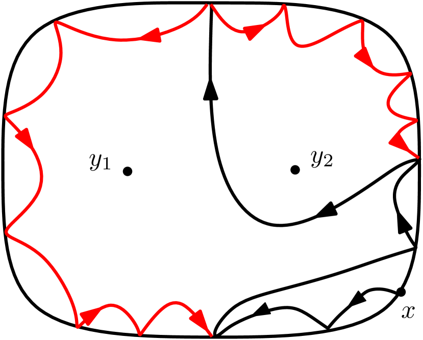

Fix . For , let be the upward height-varying sequence of level loops of with height difference starting from the boundary targeted at where is the transition step. From the above analysis, we know that there exists a number such that
(If for all , then we set .) Given , the two sequences continue towards their target points independently. We call the first disconnecting step for the two sequences and .
Fix , let be a fixed countable dense subset of . For , let be the upward height-varying sequence of level loops of with height difference targeted at . We call the union of all loops for all the upward height-varying exploration tree of with height difference , denoted by . We summarize some basic properties of the exploration tree .
-
(a)
The tree is almost surely independent of the choice of . Furthermore, it is almost surely determined by .
-
(b)
The tree is conformal-invariant: for any Möbius transformation of , we have
-
(c)
For any two points , the two upward height-varying sequences of level loops and satisfy the following property: the level loops coincide up to the first disconnecting step, after which the two sequences continue towards their target points independently.
-
(d)
For any , we denote by the connected component of that contains , or equivalently where . For any , given , the conditional law of restricted to is the same as GFF with boundary value
For any , given and on the event that , the restrictions of to and to are conditionally independent.
Now, we are ready to complete the proof of Theorem 1.2.2.
Proof of Theorem 1.2.2.
Suppose that is a zero-boundary GFF on . Fix a countable dense subset of . For , let be the upward height-varying exploration tree of with height difference . For , let be the connected component of that contains , and let be the number such that, given , the restriction of to has boundary value . From Proposition 3.4.2, we have the following observations.
-
(a)
For all , the sequence converges almost surely to some quantity, denoted by .
-
(b)
For all , the sequence converges almost surely to some loop, denoted by , in Carathéodory topology seen from .
-
(c)
For any , given , the conditional law of restricted to is the same as GFF with boundary value .
-
(d)
For any , given and on the event that , the restrictions of to and to are conditionally independent.
Combining these four facts, we have that and are coupled in the way described in Theorem 1.2.2. From Proposition 3.4.2, the collection has the same law as with time parameter. This implies the existence of the coupling. ∎
References
- [CDCH+14] Dmitry Chelkak, Hugo Duminil-Copin, Clément Hongler, Antti Kemppainen, and Stanislav Smirnov. Convergence of ising interfaces to schrammʼs sle curves. Comptes Rendus Mathematique, 352(2):157–161, 2014.
- [CS12] Dmitry Chelkak and Stanislav Smirnov. Universality in the 2D Ising model and conformal invariance of fermionic observables. Invent. Math., 189(3):515–580, 2012.
- [Dub09a] Julien Dubédat. Duality of Schramm-Loewner evolutions. Ann. Sci. Éc. Norm. Supér. (4), 42(5):697–724, 2009.
- [Dub09b] Julien Dubédat. SLE and the free field: partition functions and couplings. J. Amer. Math. Soc., 22(4):995–1054, 2009.
- [Ken08] Richard Kenyon. Height fluctuations in the honeycomb dimer model. Comm. Math. Phys., 281(3):675–709, 2008.
- [KS12] Antti Kemppainen and Stanislav Smirnov. Random curves, scaling limits and loewner evolutions. arXiv preprint arXiv:1212.6215, 2012.
- [Law05] Gregory F. Lawler. Conformally invariant processes in the plane, volume 114 of Mathematical Surveys and Monographs. American Mathematical Society, Providence, RI, 2005.
- [LSW01] Gregory F. Lawler, Oded Schramm, and Wendelin Werner. Values of Brownian intersection exponents. II. Plane exponents. Acta Math., 187(2):275–308, 2001.
- [LSW04] Gregory F. Lawler, Oded Schramm, and Wendelin Werner. Conformal invariance of planar loop-erased random walks and uniform spanning trees. Ann. Probab., 32(1B):939–995, 2004.
- [MS12] Jason Miller and Scott Sheffield. Imaginary Geometry III: Reversibility of SLEκ for . 2012.
- [MS13] Jason Miller and Scott Sheffield. Imaginary Geometry IV: Interior Rays, Whole-plane Reversibility, and Space-filling Trees. 2013.
- [MS16a] Jason Miller and Scott Sheffield. Imaginary geometry I: interacting SLEs. Probab. Theory Related Fields, 164(3-4):553–705, 2016.
- [MS16b] Jason Miller and Scott Sheffield. Imaginary geometry II: Reversibility of for . Ann. Probab., 44(3):1647–1722, 2016.
- [MW16] Jason Miller and Hao Wu. Intersections of SLE Paths: the double and cut point dimension of SLE. Probability Theory and Related Fields, pages 1–61, 2016.
- [MWW13] Jason Miller, Samuel S Watson, and David B Wilson. The conformal loop ensemble nesting field. Probability Theory and Related Fields, pages 1–33, 2013.
- [PW15] Ellen Powell and Hao Wu. Level lines of the gaussian free field with general boundary data, 2015.
- [RS05] Steffen Rohde and Oded Schramm. Basic properties of SLE. Ann. of Math. (2), 161(2):883–924, 2005.
- [Sch00] Oded Schramm. Scaling limits of loop-erased random walks and uniform spanning trees. Israel J. Math., 118:221–288, 2000.
- [She07] Scott Sheffield. Gaussian free fields for mathematicians. Probab. Theory Related Fields, 139(3-4):521–541, 2007.
- [She09] Scott Sheffield. Exploration trees and conformal loop ensembles. Duke Math. J., 147(1):79–129, 2009.
- [SS09] Oded Schramm and Scott Sheffield. Contour lines of the two-dimensional discrete Gaussian free field. Acta Math., 202(1):21–137, 2009.
- [SS13] Oded Schramm and Scott Sheffield. A contour line of the continuum Gaussian free field. Probab. Theory Related Fields, 157(1-2):47–80, 2013.
- [SW05] Oded Schramm and David B. Wilson. SLE coordinate changes. New York J. Math., 11:659–669 (electronic), 2005.
- [SW12] Scott Sheffield and Wendelin Werner. Conformal loop ensembles: the Markovian characterization and the loop-soup construction. Ann. of Math. (2), 176(3):1827–1917, 2012.
- [SWW16a] Scott Sheffield, Samuel Watson, and Hao Wu. A conformally invariant metric on cle(4), 2016.
- [SWW16b] Scott Sheffield, Samuel Watson, and Hao Wu. Simple cle in doubly connected domains, 2016.
- [WW13] Wendelin Werner and Hao Wu. On Conformally Invariant CLE Explorations. Comm. Math. Phys., 320(3):637–661, 2013.
- [WW15] Menglu Wang and Hao Wu. Level Lines of Gaussian Free Field II: Whole-Plane GFF. 2015.
- [Zha08] Dapeng Zhan. Reversibility of chordal SLE. Ann. Probab., 36(4):1472–1494, 2008.
- [Zha10] Dapeng Zhan. Reversibility of some chordal traces. J. Stat. Phys., 139(6):1013–1032, 2010.