The return of the merging galaxy subclusters of El Gordo?

Abstract

Merging galaxy clusters with radio relics provide rare insights to the merger dynamics as the relics are created by the violent merger process. We demonstrate one of the first uses of the properties of the radio relic to reduce the uncertainties of the dynamical variables and determine the 3D configuration of a cluster merger, ACT-CL J0102-4915, nicknamed El Gordo. From the double radio relic observation and the X-ray observation of a comet-like gas morphology induced by motion of the cool core, it is widely believed that El Gordo is observed shortly after the first core-passage of the subclusters. We employ a Monte Carlo simulation to investigate the three-dimensional (3D) configuration and dynamics of El Gordo. Using the polarization fraction of the radio relic, we constrain the estimate of the angle between the plane of the sky and the merger axis to be $\alpha=21\mathrm{\SIUnitSymbolDegree}\pm^{9}_{11}$. We find the relative 3D merger speed of El Gordo to be $2400\pm^{400}_{200}~{}\mathrm{k}\mathrm{m}~{}\mathrm{s}^{-1}$ at pericenter. The two possible estimates of the time-since-pericenter are $0.46\pm^{0.09}_{0.16}$ Gyr and $0.91\pm^{0.22}_{0.39}$ Gyr for the outgoing and returning scenario respectively. We put our estimates of the time-since-pericenter into context by showing that if the time-averaged shock velocity is approximately equal to or smaller than the pericenter velocity of the corresponding subcluster in the center of mass frame, the two subclusters are more likely to be moving towards, rather than away, from each other, post apocenter. We compare and contrast the merger scenario of El Gordo with that of the Bullet Cluster, and show that this late-stage merging scenario explains why the southeast dark matter lensing peak of El Gordo is closer to the merger center than the southeast cool core.

1 Introduction

Mergers of dark-matter-dominated galaxy clusters probe properties of the cluster components like no other systems. In terms of mass content, dark matter makes up $\sim 80\%$ of the mass of clusters of galaxies, a smaller portion of the mass consist of intercluster gas($\sim 15\%$ in mass content), and sparsely spaced galaxies ($\sim 2\%$ in mass content). During a merger of clusters of the high mass range of $10^{14}M_{\sun}$ to the low mass end of $10^{15}M_{\sun}$, the subclusters are accelerated to high speeds of $\sim 2000-3000~{}\mathrm{k}\mathrm{m}~{}\mathrm{s}^{-1}$ (Lage & Farrar 2014, Dawson et al. 2012). The offsets of different components of the subclusters reflect the differences in the strengths of interactions between various components. Galaxies are expected to lead the gas due to their negligible interaction cross sections with other components. The intracluster medium (ICM) is expected to lose momentum through electromagnetic interactions. On the other hand, offsets between dark matter and galaxies may suggest dark matter self-interaction (Kahlhoefer et al. 2013, Randall et al. 2008).

The galaxy cluster ACT-CL J0102-4915, (nicknamed “El Gordo”, at z=0.87), was discovered via its Sunyaev-Zel’dovich (SZ) effect by the Atacama Cosmology Telescope (ACT; Menanteau et al. 2010; Marriage et al. 2011); it has the strongest SZ effect of the full ACT survey (Hasselfield et al., 2013), and was discovered to be undergoing a major merger approximately in the plane of the sky (Menanteau et al. 2012, hereafter M12). El Gordo possesses a range of noteworthy features that allow us to constrain the merger dynamics in multiple ways.

Figure 1: Configuration of El Gordo showing overlay of dark matter distribution in blue, and X-ray emission in red. (Image credit: NASA, ESA and Jee et al. 2014). The cross markers show the positions of the northwest (NW) and southeast (SE) dark matter density peaks, and the center of mass (CM) locations respectively. Note that the mass ratio of the NW subcluster to the SE subcluster is $\sim 2:1$ (Jee et al., 2014). The dashed white lines indicate the approximate location and extent of the northwest radio relic (NW relic), the east radio relic (E relic) and the southeast radio relic (SE relic) (Lindner et al., 2014).

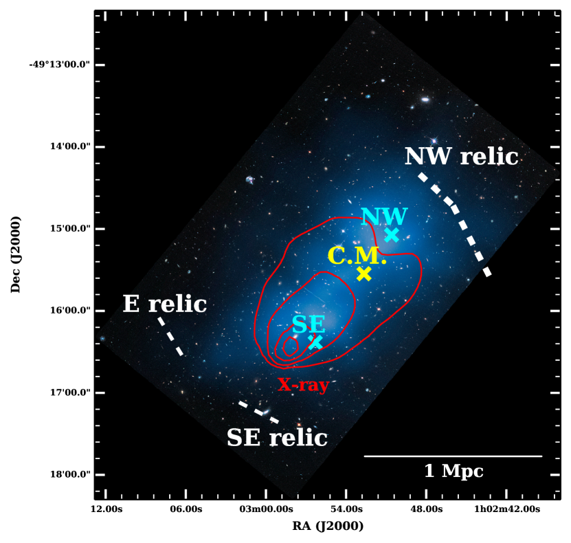
From the spectroscopy and Dressler-Schectman test for the member galaxies in Sifón et al. (2013), it is shown that El Gordo does not have complicated substructures in its galaxy velocity distribution. El Gordo is further confirmed to be a binary merger from the weak lensing analysis by Jee et al. (2014). The weak lensing analysis shows a mass ratio of $\sim$2:1 between the two main subclusters, named according to their location as the northwest (NW) and southeast (SE) subclusters respectively (See Figure 1). A bimodal distribution of cluster member galaxies is also observed (Menanteau et al., 2012). In addition, El Gordo has an interesting X-ray morphology. In the northwest, it shows a wake feature, i.e., turbulent flow due to object of higher density moving through fluids, while in the southeast, it shows the highest X-ray emissivity indicative of a cool gas core at the head of the wake. The most straightforward explanation for this morphology is that the cool gas core has passed from the northwest to the southeast (Menanteau et al., 2012). The high mass of El Gordo also makes it a good gravitational lens. Zitrin et al. (2013) have found multiple strong gravitationally lensed images around the center region of El Gordo. On the outskirts, strong radio emission is detected in the NW and the SE respectively. These radio emitting regions show steep spectral index gradients and are identified as radio relics associated with shock waves created from the merger (Lindner et al., 2014). El Gordo is one of $\sim 50$ galaxy clusters that have been associated with a radio relic and show dissociation between the X-ray gas and the DM subclusters.

Figure 2: Illustration of the spatial location of different components of El Gordo at different stages of the merger. Earlier stages (with a smaller TSP) are on the left side of later stages. The rightmost returning scenario is preferred from our simulation.

In this paper, we combined most of the available information of El Gordo with the main goal of giving estimates of the dynamical parameters after taking into account all constraints and uncertainties due to the missing variables. Since mergers of clusters proceed on the time-scale of many millions of years, one of the most important missing variables to infer is the time-since-pericenter (TSP)^†, which is defined to be the time when the mass peaks of the DM subclusters are at minimum separation. Determining the TSP of similar clusters helps us reconstruct different stages and recover the physics of a cluster merger. In particular there is a degeneracy between the following two possible scenarios: We call the scenario for which the subclusters are moving apart after pericenter to be “outgoing”, and the alternative scenario “returning” for which the subclusters are approaching each other after turning around from the apocenter for the first time (See Fig. 2).

Another crucial, missing piece of information is the 3D configuration, i.e. the angle between the plane of the sky and the merger axis called the projection angle $\alpha$. Since most of the dynamical observables are projected quantities while the modelling of physics requires 3D variables, the deprojection contributes the largest amount of uncertainty to the dynamical variables (Dawson 2013, hereafter D13). The morphology of the double relic of El Gordo suggests that $\alpha$ should be small. For mergers with a large projection angle, the radio emission would be projected towards the center of the merger, which inhibits detection (Vazza et al., 2012). However, the only quantitative constraint on $\alpha$ for El Gordo is from the analysis of the radio relic from Lindner et al. (2014) with a lower bound of $\alpha\geq 11.6\mathrm{\SIUnitSymbolDegree}$. A tighter constraint on $\alpha$ is needed for us to reduce uncertainty of the dynamical variables.

We employed a data-driven approach that thoroughly probes parameter space by directly drawing samples from the probability density functions (PDFs) of the observables. This work based on Monte Carlo simulation is particularly important since the phase space of possible merger scenarios is large. Previous attempts at modeling El Gordo with hydrodynamical simulations such as Donnert (2014) and Molnar & Broadhurst (2015) provided only in total a dozen possible configurations of El Gordo, which do not reflect the range of input uncertainties. Another approach for estimating dynamical parameters would be to look for multiple analogs of El Gordo in cosmological simulations. However, under the hierarchical picture of structure formation in the $\Lambda$CDM model, there is a rare chance for massive clusters like El Gordo to have formed at a redshift of $z=0.87$. The number density of analogs with mass comparable to El Gordo in a cosmological simulation is as low as $10^{-11}\mathrm{M}\text{pc}^{-3}$ (M12).

In the following sections, we adopt the following conventions: (1) we assume the standard $\Lambda$CDM cosmology with $\Omega_{m}=0.3$, $\Omega_{\Lambda}=0.7$ and $H_{0}=70~{}\mathrm{k}\mathrm{m}/\mathrm{s}/\mathrm{M}{\rm pc}$. (2) All confidence intervals are quoted at the 68% level unless otherwise stated. (3) All quoted masses ($M_{200c}$) are based on mass contained within $r_{200}$ where the mass density is 200 times the critical density of the universe at the cluster redshift of $z=0.87$.

Figure 3: Points showing the locations of the member galaxies and the division of the member galaxies among the two subclusters of El Gordo by a spatial cut (black line). The color of the points shows the corresponding spectroscopic redshift of the member galaxies (see color bar for matching of spectroscopic values), with the redder end indicating higher redshift. The galaxy number density contours in the background in green indicate a bimodal distribution.

2 DATA

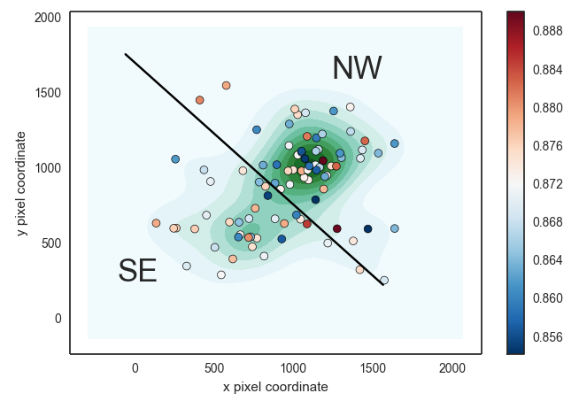
We gathered and analyzed data from multiple sources. See Table 1 for descriptions of the PDFs of the input variables. We examined the spectroscopic data obtained from the Very Large Telescope (VLT) as described in M12 and Sifón et al. (2013) for estimating the relative velocity differences between the subclusters. We adopted the identification of galaxy membership of El Gordo given by Sifón et al. (2013) with a total count of 89 galaxies. To further distinguish member galaxies of each subcluster, we adopted the spatial cut from M12. The adopted spatial cut is approximately perpendicular to the 2D merger axis (M12) and is consistent with the bimodal number density contours (See Fig. 3). There are 51 members identified in the NW subcluster and 35 members in the SE subcluster.

For the weak-lensing mass estimation, we used the Monte Carlo Markov Chains (MCMC) mass estimates from J13. The Hubble Space Telescope data used in J13 were obtained from two programs PROP 12755 and PROP 12477. PROP 12755 consisted of two pointings in the F625W, F775W, and F850LP. F850LP for a 6’ x 3’ strip, while PROP 12477 provided a $2\times 2$ mosaic pattern with F606W and a single pointing in F814W.

In order to further constrain our parameter space, we referred to the properties of the radio relics from Lindner et al. (2014). El Gordo shows radio emission on the periphery of both subclusters (M12). The two radio relics, the northwest (NW) relic and the southeast (SE) relic, of El Gordo were tentatively identified in the Sydney University Molonglo Sky Survey (SUMSS) data in low resolution at 843 MHz (Mauch et al., 2003) as shown in M12. Higher resolution radio observations conducted by Lindner et al. (2014) at 610 M Hz and 2.1 G Hz later confirmed the identities of the NW and the SE relic, and found another extended source of radio relic in the east (E) (See Fig. 1). Among the radio relics, the NW relic possesses the most extended geometry (0.56 Mpc in length), and its physics, including the polarization and Mach number, were studied in the greatest detail. Such information allows us to constrain $\alpha$ and the merger scenario. The E relic was also reported to have a resolved length of 0.27 Mpc, while the SE relic was found to overlap with a point source (Lindner et al., 2014). Both the E and SE relic are closer to the SE DM subcluster, so we considered them to originate from the same merger shock in the following work.

3 METHOD – Monte Carlo simulation

We used the collisionless dark-matter-only Monte Carlo modeling code written by D13, to model the dynamics of the DM subclusters of their first core-passage. In the D13 code, the time evolution of the head-on merger was computed based on an analytical, dissipationless model assuming that the only dominant force is the gravitational attraction from the masses of two Navarro-Frenk-White (hereafter NFW) DM halos (Navarro et al., 1996). The gravitational attraction was evaluated and summed at 10 000 fixed grid points of each of the analytic NFW halo profiles out to the respective $r_{200c}$.

In the simulation, many realizations of the collision are computed by drawing random realizations of the PDFs of the inputs. Most input variables are obtained from previous observations ($\vec{D}$). One unknown model variable, which is the projection angle between the plane of the sky and the merger axis, $\alpha$, is drawn from the PDF of $\alpha$ being observed:

$$\alpha^{(j)}\sim f(\alpha)=\cos\alpha.$$ (1)

and the calculation of the output variables of the $j$-th realization can be denoted as:

$$(\vec{\theta}^{\prime})^{(j)}=g(\alpha^{(j)},\vec{D}^{(j)}),$$ (2)

for a suitable function $g$ that describes conservation of energy during the collision of the two NFW halos due to the mutual gravitational attraction. In particular, the required $\vec{D}$ includes the masses ($M_{200_{NW}},M_{200_{SE}}$) the redshifts ($z_{NW},z_{SE}$) and the projected separation of the two subclusters ($d_{\rm proj}$). See Table 1 for quantitative descriptions of the sample PDFs, and the outputs with physical importance are described in detail in Section 3.2.

Finally, we excluded realizations that produce any unphysical output values, such as realizations with time-since-pericenter larger than the age of universe at the cluster redshift. We refer to this process of excluding unphysical realizations as applying weights. To ensure convergence of the output PDFs, in total, 2 million realizations were computed. However, the estimates would agree up to 1% just from 20 000 runs (D13). Even though we describe the weights for one variable at a time (See Appendix A), the correlations between different variables are properly taken into account since we discarded all the variables of the problematic realizations.

Table 1: Properties of the input sampling PDFs ($\vec{D}$) of the Monte Carlo simulation. We obtained estimates of the inputs via different methods. ^aWe made used of the MCMC chains from J13 for mass-related estimates (See Section 3.1.2 ). ^bThe redshift distributions were obtained from bootstrapping (See Section 3.1.1). ^cWe approximated the positions of the centroids with 2D Gaussians before we calculated the projected separations of the subclusters (See Section 3.1.3). Even though the distributions of the mass estimates and the redshift were not estimated via parametric methods (e.g. fitting mean and variances of Gaussians), they resemble Gaussian distributions due to the Central Limit Theorem.

Data	Units	Location	Scale	Ref
$M_{200c_{\mathrm{NW}}}$	$10^{14}h_{70}^{-1}$ M⊙	13.0	1.6	J13a
cNW		2.50	0.02	a
$M_{200c_{\mathrm{SE}}}$	$10^{14}h_{70}^{-1}$ M⊙	7.6	1.2	J13a
$c_{\mathrm{SE}}$		2.70	0.04	J13a
$z_{\mathrm{NW}}$		0.86842	0.00109	M12b
$z_{\mathrm{SE}}$		0.87110	0.00117	M12b
dproj	Mpc	0.74	0.007	J13c

The system of El Gordo satisfies several major assumptions in the Monte Carlo simulation. One of the strongest assumptions is that all realizations correspond to gravitationally bound systems. The simulation excludes all realizations that would result in relative pericenter velocities of the subclusters higher than the free-fall velocity. We justify our assumption of modeling only gravitationally bound systems by noting that the relative escape velocity of the subclusters for El Gordo is $4500~{}\mathrm{k}\mathrm{m}~{}\mathrm{s}^{-1}$ (based on the mass estimates of Jee et al. (2014)). Studies from cosmological simulations giving the PDFs of the pairwise velocities of massive merging clusters ($>10^{15}M_{\sun}$) indicate that it is highly unlikely that the pairwise velocities would be $>3000~{}\mathrm{k}\mathrm{m}~{}\mathrm{s}^{-1}$ under $\Lambda$CDM (Thompson & Nagamine 2012, Lee & Komatsu 2010).

Other major assumptions for modeling systems with this code include negligible impact parameter. Several papers have noted that the X-ray morphology of a bimodal merger is sensitive to the impact parameter (Springel & Farrar 2007, Ricker 1998, Mastropietro & Burkert 2008); an impact parameter as small as 0.1 Mpc can result in substantial asymmetry. The X-ray morphology of El Gordo is approximately symmetric about the merger axis. On the other hand, the dynamics of the merger is not as sensitive to the impact parameter as the X-ray morphology. The simulations of Ricker (1998) of bimodal mergers of $10^{15}M_{\sun}$ halos, showed that the resulting relative velocity would be approximately $2000\text{ km s}^{-1}$, relatively insensitive to impact parameters between 0 to 5 times the scale radius ($5~{}r_{s}=3.5$ Mpc). Mastropietro & Burkert (2008) also reported that an impact parameter of $0.1~{}r_{200}=0.14$ Mpc affected merger dynamics only at the $\sim$10% level. Molnar & Broadhurst 2015 indicated that the impact parameter of El Gordo may be as large as $40\%~{}r_{s}\approx 0.3$ Mpc, where $r_{s}$ is the corresponding characteristic core radius of the NFW halo with the mass of the SE subcluster. We attribute the result from Molnar & Broadhurst 2015 to incomplete exploration of the parameter space, and note that other impact parameter values may also match the X-ray observables of El Gordo.

Other assumptions in this simulation include negligible dynamical friction during the merger, negligible mass accretion and negligible self-interaction of dark matter. Discussion of the effects of each of these assumptions is included in D13.

3.1 Inputs of the Monte Carlo simulation

3.1.1 Membership selection and redshift estimation of subclusters

After identifying members of each subcluster, we performed 10, 000 bootstrap realizations to estimate the biweight locations of the spectroscopic redshifts of the respective members in order to obtain the samples of the PDFs of the redshifts of each subcluster. The spectroscopic redshift of the subclusters were determined to be $z_{\mathrm{NW}}=0.86842\pm 0.0011$ and $z_{\mathrm{SE}}=0.87131\pm 0.0012$, where the quoted numbers represent the biweight location and 1$\sigma$ bias-corrected confidence level respectively (Beers et al., 1990). Both the estimated redshifts of the subclusters and the uncertainties are consistent with estimates of $z=0.8701\pm 0.0009$ for El Gordo given by Sifón et al. 2013, and the fact that the member galaxies of El Gordo shows large velocity dispersion, i.e. the largest velocity dispersion among all the ACT galaxy clusters, as reported by M12.

Figure 4: Bootstrapped location of the redshift estimates and $v_{rad}$ estimates for each subcluster using the selected spectroscopic members. The shaded histograms represent the bootstrapped samples.

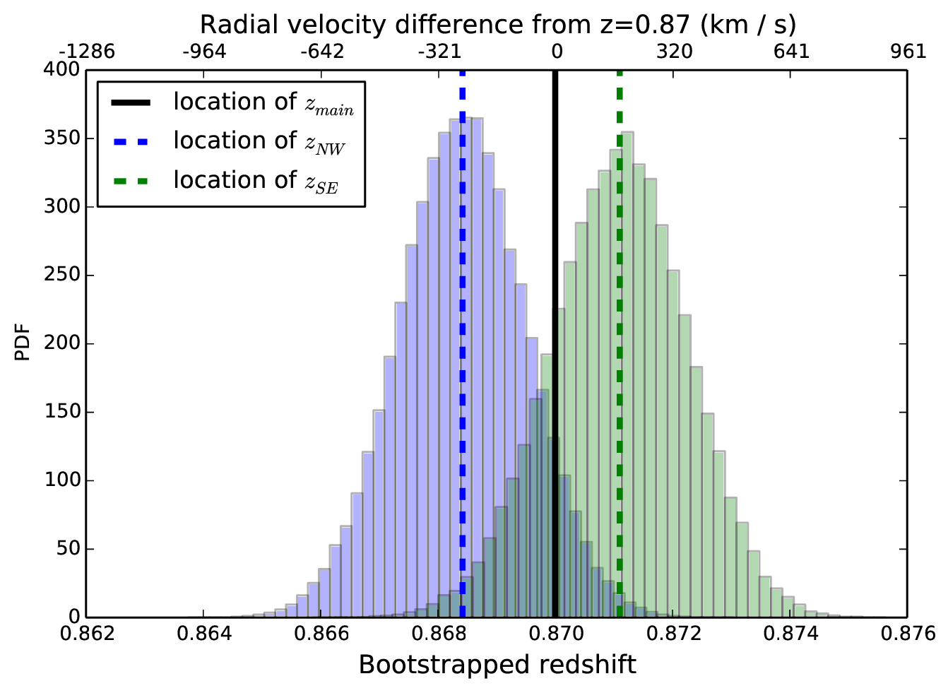
We estimated the radial velocity differences of the subclusters by first calculating the velocity of each subcluster with respect to us, using

$$v_{i}=\left[\frac{(1+z_{i})^{2}-1}{(1+z_{i})^{2}+1}\right]c,$$ (3)

where $i=1,2$ represents the two subclusters, and $c$ is the speed of light. The relative radial velocity was calculated by:

$$\Delta v_{rad}(t_{obs})=\frac{|v_{2}-v_{1}|}{1-\frac{v_{1}v_{2}}{c^{2}}}.$$ (4)

We obtained a low radial velocity difference of the two subclusters to be $476~{}\pm~{}242~{}\mathrm{k}\mathrm{m}~{}\mathrm{s}^{-1}$ (See Fig. 4). The radial velocity difference of $586~{}\mathrm{k}\mathrm{m}~{}\mathrm{s}^{-1}$ reported by M12 is higher than our estimates but within the 68% bias-corrected confidence interval.

3.1.2 Weak lensing mass estimation

We obtained 40, 000 samples of the joint PDFs of the masses of the two dark matter halos as the outputs of the Monte Carlo Markov Chain (MCMC) procedure from Jee et al. 2014. Discussion of the handling of the weak lensing source galaxies and the details of the MCMC procedure for mass estimation can be found in Jee et al. 2014.

3.1.3 Estimation of projected separation ($d_{\rm proj}$)

To be consistent with our MCMC mass inference, our Monte Carlo simulation takes the projected separation of the NFW halos to be those of the inferred DM centroid locations in Jee et al. 2014. We drew random samples of the location of centroids from two 2D Gaussians centered at R.A.$=$01:02:50.601, Decl.=$-$49:15:04.48 for the NW subcluster and R.A. = 01:02:56.312, Decl.=$-$49:16:23.15 for the SE subcluster, with a 1” standard deviation each as estimated from the convergence map of Jee et al. (2014). The inferred centroid locations correspond to a mean projected separation ($d_{\rm proj}$) of $0.74\pm{0.007}$ Mpc.

3.2 Outputs of the Monte Carlo simulation

We outline the outputs of the simulation here to facilitate the discussion of the design of the weights used in the simulation. The simulation provides PDF estimates for 8 output variables. Variables of the highest interest include the time-since-pericenter and the angle $\alpha$, which is defined to be the projection angle between the plane of the sky and the merger axis. Other output variables are dependent on $\alpha$ and time. Specifically, the simulation denotes the time dependence by providing several characteristic time-scales, including the time elapsed between consecutive collisions ($T$) and the time-since-pericenter of the observed state ($TSP$), with the time of pericenter defined to be when the centers of the two NFW halos coincide.

We provide two versions of the time-since-pericenter variables $TSP_{\rm out}$ and $TSP_{\rm ret}$ to denote different possible merger scenarios. 1) The TSP for the“outgoing” scenario corresponds to the smaller $TSP_{\rm out}$ value, and 2) the “returning” scenario corresponds to the larger $TSP_{\rm ret}$. We describe how we make use of properties of the radio relic to evaluate which scenario is more likely in section 3.4. Evolution of the merger after the second passage is not considered. Outputs from our dissipationless simulation for a “second” passage will not differ from the first passage, and the predicted relic position would be so far for us to rule this out.

The simulation also outputs estimates of variables that describe the dynamics and the characteristic distances of the merger. The relative 3D velocities of the subclusters, both at the time of the pericenter ($v_{3D}(t_{\rm per})$) and at the time of observation ($v_{3D}(t_{obs})$) are provided. The characteristic distances included in the outputs are the maximum 3D separation ($d_{max}$), which is the distance between the subclusters at the apocenter and the 3D separation of the subclusters at observation ($d_{3D}$).

3.3 Design and application of weights

One of the strengths of the Monte Carlo simulation by D13 is its ability to detect and rule out extreme input values that would result in unphysical realizations via the application of weights. Our default weights are described in D13 and we include them in Appendix 10 for the convenience of the readers. In addition, we have devised a new type of weights of the projection angle $\alpha$ based on the polarization fraction of the radio relic.

3.3.1 Monte Carlo weights based on the polarization fraction of the radio relic

We can relate the polarization fraction of the radio relic to the projection angle by examining the generating mechanism of the radio relic. The observed radio relic was generated by synchrotron emission of free electrons in a magnetic field. If the magnetic field was uniform, the observed polarization fraction of the synchrotron emission of the electrons depends on the viewing angle (or equivalently the projection angle) with respect to the alignment of the magnetic field. Synchrotron emission from electrons inside unorganized magnetic field is randomly polarized. The high reported integrated polarization fraction from Lindner et al. (2014) can be explained by a highly aligned magnetic field, compressed along with the ICM during a merger (Ensslin et al. 1998, van Weeren et al. 2010, Feretti et al. 2012).

We designed the weights to reflect how $\alpha$ decreases monotonically as the maximum observable integrated polarization fraction ($\langle P\rangle$).

Figure 5: Predictions of polarization percentage of the radio relic at a given projection angle from different models, reproduced from (Ensslin et al., 1998) or equation 5. Each model assumes electrons producing the radio emission to be accelerated inside uniform magnetic field of various strengths (strong or weak). The curves are plotted with spectral index of the radio emission ($\alpha_{radio}$), spectral index of the electrons ($\gamma$) and compression ratio of the magnetic field ($R$) corresponding to the estimated values from Lindner et al. (2014). We highlight the observed polarization percentage of the main NW radio relic of El Gordo by the dotted vertical line with the greyed out region indicating the uncertainty (Lindner et al., 2014).

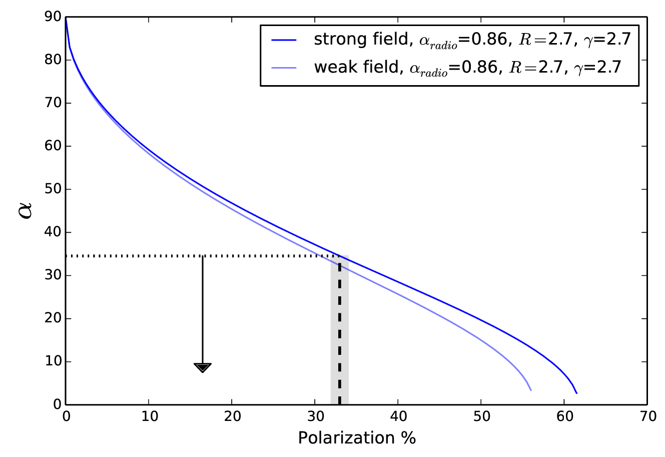
This assumption is based on the class of models given by Ensslin et al. (1998)(See Figure 5). In particular, we refer to a model from Ensslin et al. (1998) that would give the most conservative estimate on the upper bound of $\alpha$:

$$\alpha=90\mathrm{\SIUnitSymbolDegree}-\arcsin\left(\sqrt{\frac{\frac{2}{15}\frac{13R-7}{R-1}\frac{\gamma+7/3}{\gamma+1}\langle P_{strong}\rangle}{1+\frac{\gamma+7/3}{\gamma+1}\langle P_{strong}\rangle}}\right),$$ (5)

This model corresponds to the case of a strong field with the relic being supported by magnetic pressure only, with the spectral index of the radio emission being $\alpha_{radio}=0.86$, the compression ratio of the magnetic field being $R=2.7$ and the spectral index of the electrons being $\gamma=2.7$ (Lindner et al., 2014). This model predicts a maximum integrated polarization fraction of $\sim 60\%$ when $\alpha\rightarrow 0$. This polarization fraction of $\sim 60\%$ predicted by (Ensslin et al., 1998) is consistent with the upper bound of relic polarization fraction in cosmological simulations (Skillman et al., 2013). From this model, the observed integrated polarization fraction of $33\%\pm 1\%$ corresponds to an estimated value of $\alpha=35\mathrm{\SIUnitSymbolDegree}$. No other model of the magnetic field should predict a higher polarization fraction, thus it is highly unlikely that we see 33% integrated polarization at $\alpha>35\mathrm{\SIUnitSymbolDegree}$.

We cannot rule out $\alpha\leq 35\mathrm{\SIUnitSymbolDegree}$ because magnetic field nonuniformities can lower the polarization below the Ensslin model value. Ensslin et al. (1998) assumes an isotropic distribution of electrons in an isotropic magnetic field. Cosmological simulations of radio relics from Skillman et al. (2013) show varying polarization fraction across and along the relic assuming $\alpha=0$, resulting in a lower integrated polarization fraction. For example, it is possible to see an edge-on radio relic ($\alpha=0$) with integrated polarization fraction of 33%. Furthermore, Skillman et al. (2013) shows that after convolving the simulated polarization signal with a Gaussian kernel of 4 ′ to illustrate effects of non-zero beam size, the polarization fraction drops to between 30% to 65% even when $\alpha=0$. We examined the effects of perturbing the cutoff value of this weight to ensure the uncertainties do not introduce significant bias in the estimated output variables in section 4.2. To summarize, we used a conservative uniform weight to encapsulate the information from the polarization fraction of the radio relic as:

$$w(\alpha)=\begin{cases}&\text{const. for }\alpha<35\mathrm{\SIUnitSymbolDegree}\\ &0\text{ otherwise,}.\end{cases}$$ (6)

We refer to equation 6 as the polarization weights. Unless otherwise stated, the main results of the paper are obtained after applying this polarization weight in addition to the default weights.

3.4 Extension to the Monte Carlo simulation - Determining merger scenario with radio relic position by model comparison

Table 2: List of variables that provide quantitative constraints for the merger scenario. For details of the distribution of each variable see the corresponding ^†Section. Calculations were done with all available realizations instead of the best estimate value listed here.

Variable	Best estimate value	Unit	Section†
Time averaged speed of SE relic in the CM frame ($\langle v_{relic}\rangle$)	530	km s-1	4.1
Time averaged speed of NW relic in the CM frame ($\langle v_{relic}\rangle$)	310	km s-1	4.1
Projected separation of SE relic from the CM ($s_{proj}$)	1.1	Mpc	3.4
Projected separation of NW relic from the CM ($s_{proj}$)	0.63	Mpc	3.4
Outgoing time-since-pericenter ($TSP_{out}$)	0.61	Gyr	3.2, 4.1
Returning time-since-pericenter ($TSP_{ret}$)	1.0	Gyr	3.2, 4.1
Age of the universe at z = 0.87	6.30	Gyr
Free fall velocity of subclusters	4500	km s-1	3
Polarization fraction of NW relic ($\langle P_{strong}\rangle$)	33%		3.3.1

One of the biggest questions involving the merger is whether El Gordo is observed during a returning or outgoing phase. We compared the two merger scenarios by making use of the observed projected separation of the relic from the center of mass. Simulations of cluster mergers such as the work of Paul et al. (2011), Van Weeren et al. (2011), and Springel & Farrar (2007) showed that merger shock fronts that may correspond to the radio relics 1) are generated near the center of mass of the subclusters close to the time of the first core-passage, 2) propagate outward with the shock speed decreasing only slightly. The propagation speed of the shock wave with respect to the center-of-mass is reported to drop between $\sim 10\%$ from Springel & Farrar (2007) and 10% to 30% from Paul et al. (2011) (note that the time resolution is 0.6 Gyr for the simulation in Paul et al. 2011).

To capture the monotonically decreasing trend of the propagation speed of the shock fronts with respect to the center of mass, we expressed the possible time-averaged shock speeds as a factor of the inferred pericenter speed of the corresponding subcluster in the center of mass frame. Then we calculated how far the shock would have propagated for our inferred $TSP_{\rm out}$ and $TSP_{\rm ret}$ values. We worked in the center of mass frame where the shock speed is expected to drop slightly with TSP. The projected separation of the shock is approximated as:

$$s^{j}_{proj}\approx\langle v_{relic}\rangle^{j}(t^{j}_{obs}-t^{j}_{per})\cos(\alpha^{j}),$$ (7)

where the superscript $j$ of any variable denotes the value of the variable from the j-th realization of the simulation, and $s_{proj}$ is the estimated projected separation. We estimated the upper and lower bounds of the time-averaged velocity $\langle v_{relic}\rangle$ of the shock between the pericenter of the subclusters and the observed time as:

$$\langle v_{NWrelic}\rangle^{j} =\beta~{}v^{j}_{3D,NW}(t_{\rm per})$$ (8)

$$=\beta~{}v^{j}_{3D}(t_{\rm per})\frac{m^{j}_{SE}}{m^{j}_{SE}+m^{j}_{NW}},$$ (9)

where $\beta$ is a factor that we introduce to represent the uncertainty of the velocity of the relic shock wave, $v_{3D,NW}(t_{\rm per})$ refers to the pericenter velocity of the NW subcluster in the center-of-mass frame as a comparison, and $m$ represents the mass within $r_{200c}$ of each subcluster as denoted by the labels in the subscripts. Likewise, we have also computed the expected projected separation of the SE relic using:

$$\langle v_{SErelic}\rangle^{j}=\beta~{}v^{j}_{3D}(t_{\rm per})\frac{m^{j}_{NW}}{m^{j}_{SE}+m^{j}_{NW}}.$$ (10)

Figure 6: The marginalized output PDF of the returning time-since-pericenter ($TSP_{\rm ret}$) vs. the 3D velocity at the time of pericenter for El Gordo. The grey set of contours show the confidence regions before applying the polarization weight and the colored contours correspond to the confidence regions after applying the weights. The contours represent the 95% and 68% confidence regions respectively.

Table 3: Table of the output PDF properties of the model variables and output variables from Monte Carlo simulation

				Default weights				Default + polarization weights
Variables	Units		Location	68$\%$ CI †	95$\%$ CI		Location	68$\%$ CI	95$\%$ CI
$\alpha$	(degree)		43	19-69	6-80		21	10-30	3-34
$d_{\rm proj}$	Mpc		0.74	0.74-0.75	0.73-0.76		0.74	0.74-0.75	0.73-0.76
$d_{\rm max}$	Mpc		1.2	0.90-2.2	0.77-4.6		0.93	0.81-1.2	0.75-1.9
$d_{\rm 3D}$	Mpc		1.0	0.79-2.1	0.75-4.3		0.80	0.76-0.88	0.74-0.91
$TSP_{\rm out}$	Gyr		0.61	0.4-0.95	0.26-2.4		0.46	0.30-0.55	0.21-0.64
$TSP_{\rm ret}$	Gyr		1.0	0.77-1.7	0.63-4.4		0.91	0.69-1.3	0.59-2.3
$T$	Gyr		1.6	1.3-2.4	1.2-6.4		1.4	1.2-1.6	1.2-2.2
$v_{\rm 3D}(t_{\rm obs})$	k m   s -1		580	260-1200	59-2400		940	360-1800	62-2900
$v_{\rm rad}(t_{\rm obs})$	k m   s -1		360	140-630	27-880		310	110-590	8-840
$v_{\rm 3D}(t_{\rm per})$	k m   s -1		2800	2400-3700	2100-4200		2400	2200-2800	2100-3500

$\dagger$ CI stands for confidence interval

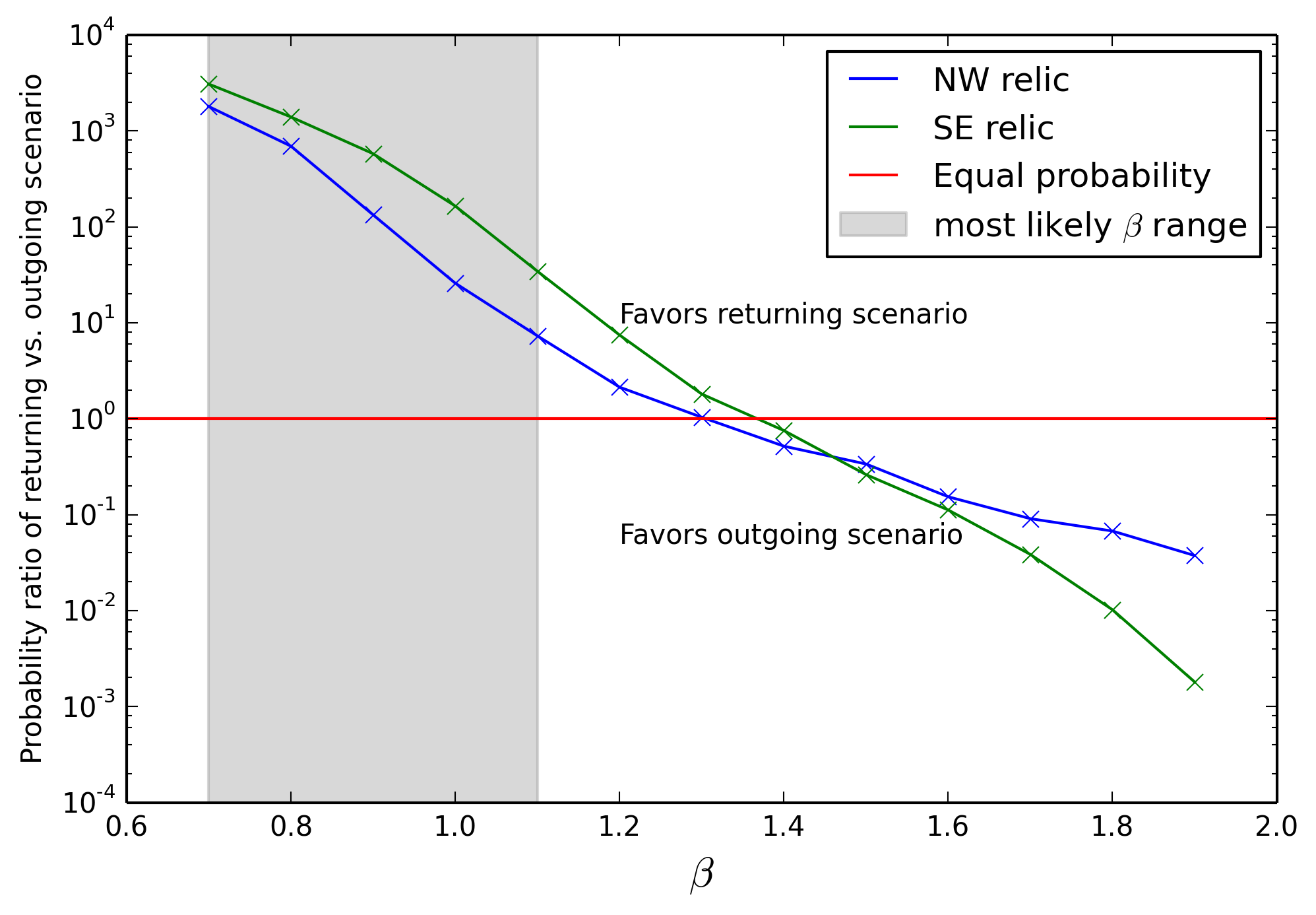
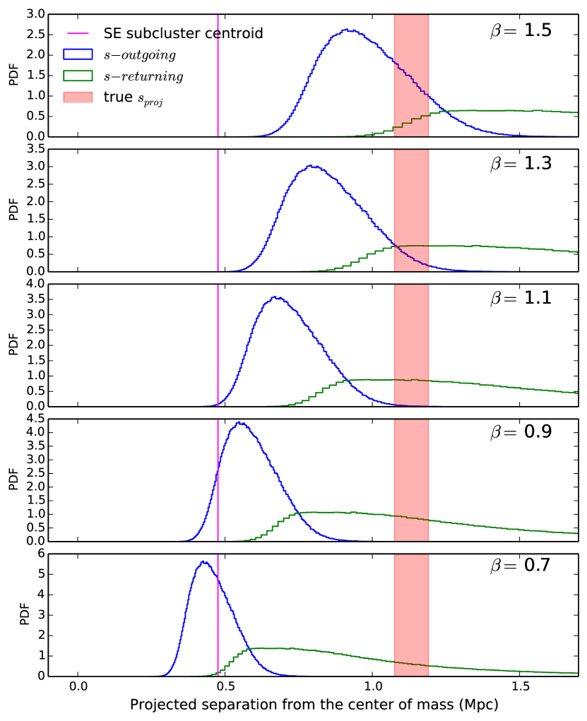
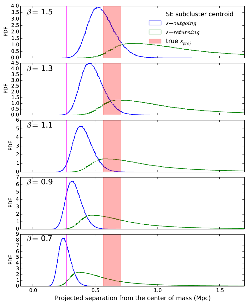
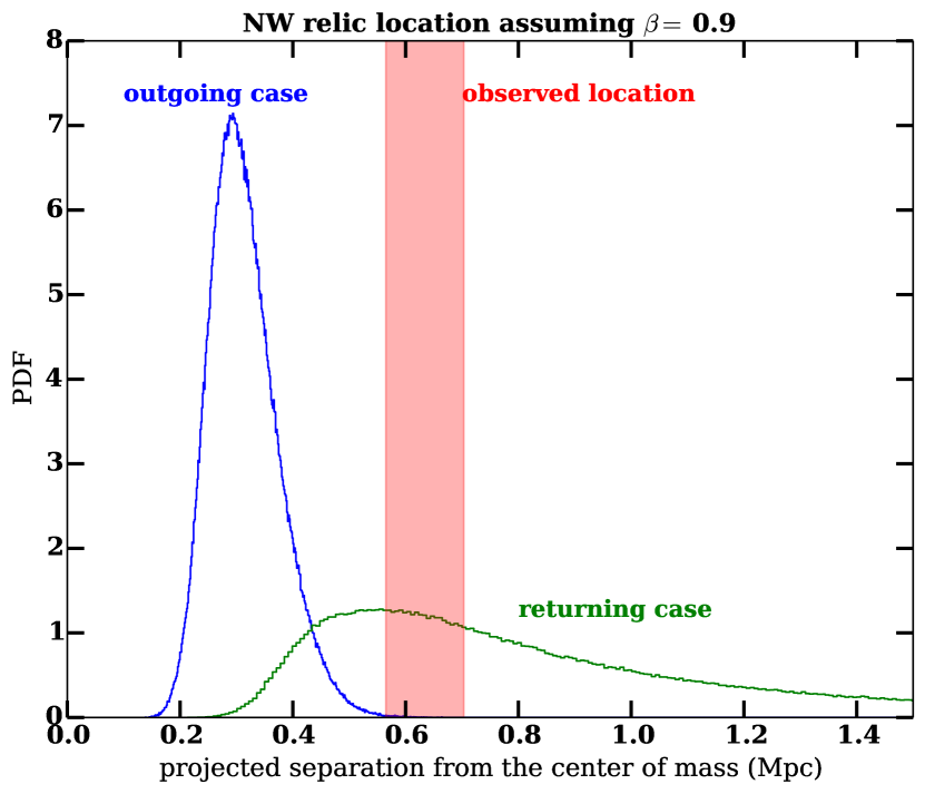
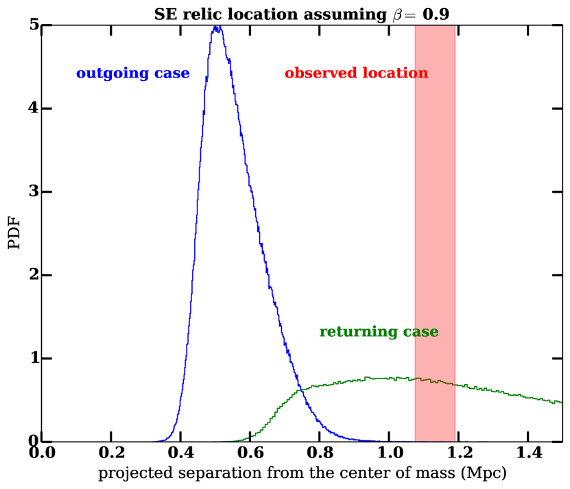
For the most likely range of $\beta$, we refer to the simulations of cluster mergers by both Springel & Farrar (2007) and Paul et al. (2011) because those are some of the few simulations available that quote shock propagation speeds in the center-of-mass frame of the cluster, rather than the ICM frame. The simulation of the Bullet Cluster by Springel & Farrar (2007), indicates that the propagation velocity of the shock evolves such that $\beta\approx 0.95$ within $\sim 0.4~{}\mathrm{G}$yr after the pericenter. For the analysis of El Gordo, we suggest $\beta\approx 0.9$ to be the most likely value given that the $TSP$ of El Gordo is longer. To include the possible range of valid $\beta$ values, we examined $0.7\leq\beta\leq 1.5$. This range of $\beta\approx 1$ allows us to use equations 8 and 10 to reflect that the shock is driven by the merger. We note that the propagation speed of the shock is also determined by the temperature, density and other details of the gas medium (Prokhorov & Durret 2007, Springel & Farrar 2007, Milosavljević et al. 2007), so it is physically possible for the shock to propagate with $\beta>1$. An example of merging clusters (Merger F) with $\beta\approx 2.0$ has been reported by the cosmological simulations in Paul et al. 2011. However, we note that Merger F from Paul et al. 2011 has a lower mass of $\sim 1.1\times 10^{14}M_{\sun}$ in total, and that the coarse time resolution in Paul et al. 2011 likely underestimates the pericenter velocity and overestimates $\beta$. We therefore suggest a most likely range, closer to the value of $\beta$ inferred from Springel & Farrar (2007), as $0.7\leq\beta\leq 1.5$. In section 4.1, we demonstrate that $\beta$ has to be larger than $1.5$ to avoid the returning model, and in Appendix  C, we show the full range of possibilities up to $\beta=2.0$. In fig. 7 and 8, we compared our estimates of the projected locations of the relics to the observed location given by Table 3 of L13. The given NW relic and E relic locations are R.A.=01:02:46, Decl.=$-$49:14:43 and R.A.=01:03:07, Decl.=$-$49:16:16 respectively. These locations correspond to a projected separation of 0.63 Mpc (NW relic) and 1.1 Mpc (E relic) from the center of mass.

4 RESULTS

We present an overview of all the estimated variables in Table 3, with results only applying the default weights on the left hand side of the table and those also applied with the polarization weight on the right hand side. Furthermore, we include the plots of all the marginalized PDFs with the polarization weight in Appendix 10.

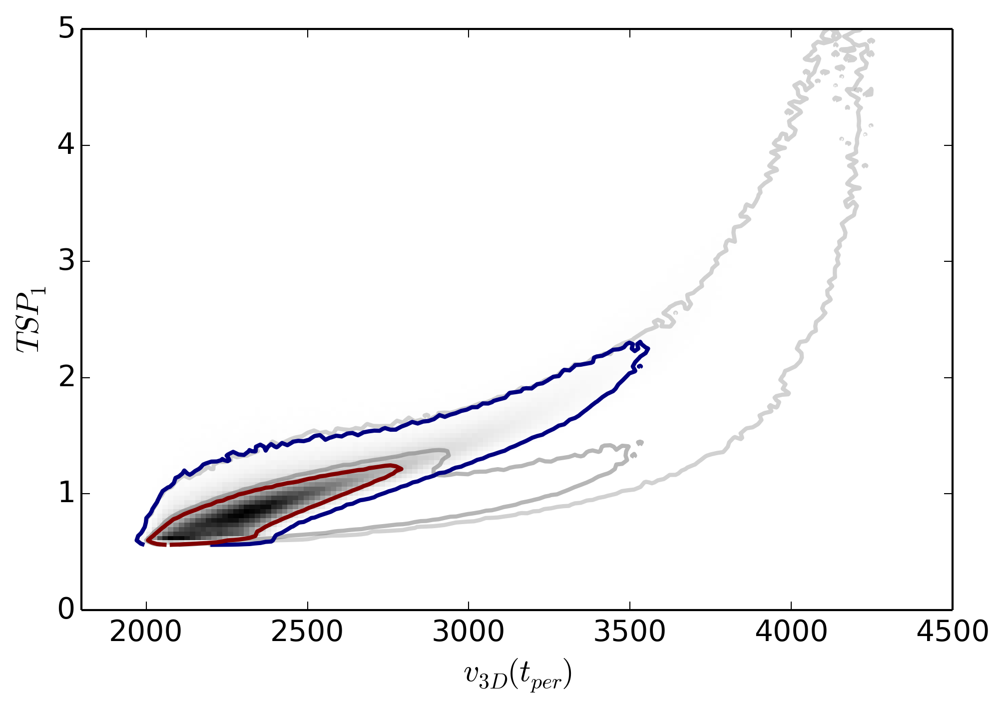
We found that the two subclusters collided with a relative velocity of $2400\pm^{900}_{400}~{}\mathrm{k}\mathrm{m}~{}\mathrm{s}^{-1}$, at an estimated projection angle of $\alpha=21\mathrm{\SIUnitSymbolDegree}\pm^{9}_{11}$. From our analysis of the two scenarios, we found that El Gordo is more likely to be observed at a returning phase with an estimate of $TSP_{\rm ret}=0.91\pm^{0.22}_{0.39}$ Gyr (See section 4.1 and Appendix C for a full discussion of the assumed relic propagation speed). This returning scenario puts the estimate of the time of pericenter to be when the age of the universe was $\sim 5.4$ Gyr. Our estimate of $v_{3D}(t_{obs})$ is $940\pm^{860}_{580}~{}\mathrm{k}\mathrm{m}~{}\mathrm{s}^{-1}$. (See Fig. 6) This fits comfortably within the upper limit of $2500\pm^{400}_{300}\mathrm{k}\mathrm{m}~{}\mathrm{s}^{-1}$ reported by Lindner et al. (2014), which was obtained by making use of the Mach number of the NW radio relic.

4.1 Time-since-pericenter (TSP) and the merger scenario

The simulation gives two estimates for the time-since-pericenter, with $TSP_{\rm out}=0.46\pm^{0.09}_{0.16}~{}\mathrm{G}\text{yr}$ and $TSP_{\rm ret}=0.91\pm^{0.39}_{0.22}~{}\mathrm{G}\text{yr}$ for the returning model. Both the estimates of $TSP_{\rm out}$ and $TSP_{\rm ret}$ fit within the observable time scale of the radio relics, which is on the scale of $\sim 1~{}\mathrm{G}$yr.

Based on section 3.4, we present the PDF of $d_{\rm proj}$ using the most likely value of $\beta=0.9$ in Fig. 7 and  8 to show that the returning model is preferred for both the calculations of the NW and the SE relic. This conclusion favoring the returning model ($M_{ret}$) holds true for the relevant range of $\beta<1.1$, which corresponds to the time-averaged velocity of the relics at $\langle v_{NWrelic}\rangle<1000~{}\mathrm{k}\mathrm{m}~{}\mathrm{s}^{-1}$ and $\langle v_{SErelic}\rangle<1800~{}\mathrm{k}\mathrm{m}~{}\mathrm{s}^{-1}$ in the center of mass frame. For comparison, we found that an extreme, and unlikely range of $\beta>1.5$ would be needed for the outgoing scenario($M_{out}$) to be preferred. (See Appendix C for plots of the range of $\beta$ that we examined). We marginalized $\beta$ to compute the probability of the simulated relic location being compatible with the observed location $P(S_{proj}\cap S_{obs}|M)$. We then computed $P(S_{proj}\cap S_{obs}|M_{ret})/P(S_{proj}\cap S_{obs}|M_{out})$. The ratio of the two probabilities is found to be $\approx 2.1$ for the NW relic and a relative probability of $\approx 460$ for the SE relic, favoring the returning scenario despite the uncertainties. (See appendix C). This scenario is further supported by the position of the cool core in the southeast as discussed in Section 5.

Finally, we note that the estimate of NW shock velocity at $2500\pm^{400}_{300}~{}\mathrm{k}\mathrm{m}~{}\mathrm{s}^{-1}$ by Lindner et al. (2014) was inferred from the Mach number, thus, this velocity is measured in the reference frame of the turbulent ICM, not the velocity with respect to center of mass. Due to the difference that could arise from the different frame of references, we have not made use of the Mach number estimate of Lindner et al. (2014) in this calculation. If there are radio data in more frequency bands than the radio data available now (Lindner et al., 2014), an alternative constraint of the TSP can be constructed from the spectral aging of the electrons that were involved in the generation of the radio relics, such as shown in Stroe et al. (2014).

Figure 7: Comparison of the PDFs of the observed position of the NW relic (red bar includes the 95% confidence interval of location of the NW radio relic in the center of mass frame) with the predicted position from the two simulated merger scenarios (blue for outgoing and green for the returning scenario). We made use of the polarization weight for producing this figure. The rationale of picking $\beta=0.9$ can be found in the last paragraph of section 3.4.

Figure 8: Comparison of the PDFs of the observed position of the SE relic (red bar includes the 95% confidence interval of location of the radio relic in the center of mass frame). We made use of the polarization weight for producing this figure. The rationale of picking $\beta=0.9$ can be found in the last paragraph of section 3.4.

4.2 Sensitivity analysis of the polarization weight

We performed tests of how the output variables vary according to the choice of the cutoff of the polarization weight between $\alpha_{\text{cutoff}}=29\mathrm{\SIUnitSymbolDegree}$ to $49\mathrm{\SIUnitSymbolDegree}$ instead of $35\mathrm{\SIUnitSymbolDegree}$, that is, shown as the horizontal cut off in Fig. 5. We found that in the most extreme case, choosing the cutoff values as $29\mathrm{\SIUnitSymbolDegree}$, the location of the $v_{3D}(t_{obs})$, is increased by $16\%$. While the $95\%$ CI of $d_{max}$ is the most sensitive to the weight and it changes by $\sim 20\%$ when $\alpha_{\text{cutoff}}=49\mathrm{\SIUnitSymbolDegree}$. This shows that the exact choice of the cut off value for $\alpha$ for the polarization weight does not change our estimates drastically.

5 DISCUSSION

5.1 Comparison of our study with other studies of El Gordo

We outline the qualitative agreement and disagreement between our simulations and hydrodynamical simulations of El Gordo such as Donnert (2014) and Molnar & Broadhurst (2015). Our simulation focuses on giving PDF estimates of particular dynamical and kinematic variables, whereas the hydrodynamical simulations focused on understanding the detailed gas dynamics required to reproduce the X-ray observables and SZ observables of El Gordo. The goals, assumptions, and initial conditions of Donnert (2014) and Molnar & Broadhurst (2015) differ substantially with ours. However, our approach has the advantage of considering a much wider range of geometries and dynamical parameters, and is based on recently measured lensing masses.

Both hydrodynamical simulations were based on a few sets of initial conditions, instead of thorough sampling of the inputs. For example, both simulations made use of the mass estimates from the dynamics analysis of M12 at $m_{NW}=1.9\times 10^{15}M_{\sun}$, which is larger than the upper 95% CI of the mass that we used based on the weak lensing estimate. Furthermore, Molnar & Broadhurst (2015) initialized the relative infall velocity (velocity when the separation of subclusters equals the sum of the two virial radii) to be $2250~{}\mathrm{k}\mathrm{m}~{}\mathrm{s}^{-1}$. This corresponds to $v_{3D}(t_{\rm per})\gtrsim 4700~{}\mathrm{k}\mathrm{m}~{}\mathrm{s}^{-1}$, which is close to the escape velocity of the subclusters. Our simulation shows a negligible number of realizations with $v_{3D}(t_{\rm per})>3000~{}\mathrm{k}\mathrm{m}~{}\mathrm{s}^{-1}$. The range of projection angles suggested by Molnar & Broadhurst (2015) of $\alpha\gtrsim 45\mathrm{\SIUnitSymbolDegree}$ is also excluded by our polarization weight, whereas we are unable to find information concerning the projection angle of the simulation from Donnert (2014).

With a time resolution of 0.25 $\mathrm{G}$yr, Donnert (2014) gave an estimate of $T\approx 2~{}\mathrm{G}$yr between the first and second core-passage in Fig. 6 of their work, while our estimate gives $T=1.4\pm{0.2}~{}\mathrm{G}$yr. By matching the simulated X-ray luminosity and the projected separation of $0.69$ Mpc to the corresponding observables, Donnert (2014) also reported their simulated work to best match observations at $\sim 0.15~{}\mathrm{G}$yr after pericenter. The $TSP_{\rm out}$ from Donnert (2014) is below the estimated 95% CI of $TSP_{\rm out}$ from our work. On the other hand, Donnert (2014) obtained a relative pericenter velocity between the subclusters at $\sim 2600~{}\mathrm{k}\mathrm{m}~{}\mathrm{s}^{-1}$, which is compatible with our estimate of $2400\pm^{400}_{200}~{}\mathrm{k}\mathrm{m}~{}\mathrm{s}^{-1}$. This agreement might be due to the similar assumptions of a low energy orbit and a small impact parameter as the initial conditions in the work of Donnert (2014) and our work. Ideally, the hydrodynamic and Monte Carlo dynamical approaches should be combined, with new hydrodynamic simulations seeded with initial conditions motivated by the results presented here.

5.2 Comparison to the merger scenarios of other merging clusters of galaxies

Figure 9: Schematic evolution of cool core gas and DM displacements relative to the merger center of mass as a function of the phase ($TSP/T$), based on simulations of a bimodal cluster merger by Mathis et al. (2005). During and shortly after core passage, ram pressure ($=\rho v^{2}$) exerts substantial force on the cool core, which then lags the DM. (This corresponds to the outgoing scenario of $TSP_{\rm out}/T$ indicated by the grey dotted line). Ram pressure then declines dramatically as the cool core enters regions of lower density. The cool core can then fall into (and past the center of) the gravitational potential of the corresponding DM subcluster as what is described as the slingshot effect (Markevitch & Vikhlinin, 2007). The Bullet Cluster is seen at a phase of $TSP_{\rm out}/T\approx~{}0.4\text{ Gyr}/~{}1.6\text{ Gyr}$ after core passage according to (D13) and indeed the cool core is closest to the center of mass. We found that El Gordo is more likely to be seen at a later stage (as indicated by $TSP_{\rm ret}/T$ rather than $TSP_{\rm out}/T$), explaining why the DM of El Gordo is closer to the center of mass than the cool core.

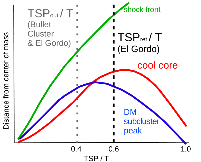
The hypothesis of El Gordo being in the returning phase is more plausible when we compare the details of the observables of El Gordo to the Bullet Cluster (Bradač et al. 2006, Springel & Farrar 2007, Mastropietro & Burkert 2008). Many inferred properties are similar between the two clusters and both clusters were observed in similar wavelengths. Both clusters are bimodal major mergers of subclusters of substantial masses. The inferred merger velocities are comparable at around $2600~{}\mathrm{k}\mathrm{m}~{}\mathrm{s}^{-1}$ and $\alpha$ of both clusters are around $20\mathrm{\SIUnitSymbolDegree}$. In particular, the inferred outbound $TSP_{\rm out}/T\sim 0.3$ of the Bullet Cluster and El Gordo are similar. If instead, the El Gordo is in the returning phase of the merger (i.e. $TSP_{\rm out}$ for El Gordo is invalid) while the Bullet Cluster is in the outgoing phase, the differences in the observables of El Gordo and the Bullet Cluster can be explained.

First, the merger shock front of the Bullet Cluster is observed only in the X-ray, but not via the radio relic, meaning that the shock may not have the time to propagate to the outskirts of the cluster (Brüggen et al. 2011, Markevitch & Vikhlinin 2007), and this bow shock is indeed observed to closely lead the corresponding less massive subcluster by $\sim 0.08~{}\mathrm{M}$pc, assuming they are propagating outward. On the other hand, indirect observables of the merger shocks of El Gordo can only be detected through the radio relic, and the shock is further offset from the corresponding subcluster ($\sim 0.5~{}\mathrm{M}$pc) and the cool core ($\sim 0.4~{}\mathrm{M}$pc).

Second, for the Bullet Cluster, the cool core (or the bullet) is closer to the interior of the system than the corresponding less massive DM subcluster mass peak, whereas the cool core of El Gordo is further offset from the center of mass than the corresponding SE subcluster (See Fig. 1 for the observed positions). Both configurations of cool core relative to the subcluster mass peak are mentioned in Markevitch & Vikhlinin (2007), with the case of the Bullet Cluster explained by the ram pressure stripping effect, and the case of El Gordo explained by the ram pressure slingshot effect, which only occurs at a later stage of a merger (See Fig. 9 for a schema depicting this conjectured scenario).

Simulation of a major merger by Mathis et al. (2005) with comparable mass ($1.4\times 10^{15}M_{\sun}$) and mass ratio (1:1) as El Gordo supports our proposed scenario: it shows the turn-around of the cool core can occur after the apocenter of the DM component, resulting in the cool core being further away from the center of mass than the dark matter by as much as $\sim 0.2~{}\mathrm{M}$pc. The gas northwest of the cool core of El Gordo shows a comet-like morphology with two tails that suggests outbound motion of the cool core, which may seem contradictory to the returning scenario. However, from our proposed merger scenario of El Gordo in Figure 9, it is possible that the cool core and the DM are observed to be moving in opposite directions, with the DM subcluster started returning for a second core-passage. If the returning scenario is true, El Gordo would be one of the first clusters shown to be observed at a returning phase of the merger, after another bimodal cluster merger A168 with a cool front leading the corresponding DM subcluster (Hallman & Markevitch, 2004).

5.3 El Gordo as a probe of dark matter self-interaction

El Gordo possesses a range of special properties that make it a promising probe of self-interaction of DM. Its high mass ensures high DM particle density for interactions during the high-speed core-passage. Its bimodal configuration makes it relatively simple to interpret the offset and dynamics of the different components. The observation of the radio relic has enabled us to constrain the projection angle and reduce uncertainties of other dynamical parameters. Furthermore, El Gordo is likely to be a late-stage merger unlike other well studied clusters such as the Bullet Cluster. This gives us a better picture of how a bimodal merger would behave at a later stage of a merger.

This special merger scenario of El Gordo also raises a question: what phase of a merger or what type of mergers would allow the most stringent constraints on the self-interaction cross section of DM ($\sigma_{\text{SIDM}}$)? The use of merging clusters as probes of $\sigma_{\text{SIDM}}$ has been proposed and used in various papers. (Markevitch et al. 2004, Randall et al. 2008, Merten et al. 2011, Dawson et al. 2012). One common theme among such work is to make use of the observed offsets of the different components of the merging clusters for the estimation. One of the most popular methods proposed by Markevitch et al. 2004 (method 1 in the paper) assumes the gas component would lag behind the corresponding DM subcluster along the direction of motion due to ram pressure stripping. For El Gordo, since the cool core is further away from the center of mass than the SE DM centroid, it is apparent that this particular method does not apply.

Alternative methods for determining the self-interaction cross sections, such as from the galaxy-DM offset, are yet to be perfected. Future work is required to investigate how to best characterize the spatial distribution of the galaxies. One pending question is to investigate if the luminosity density peak or number density peaks would better represent the galaxy distributions. The galaxy number density map of El Gordo (J13) shows a noteworthy $\sim 0.2~{}\mathrm{M}$pc offset between the SE galaxy number density peak and the SE DM centroid, while there is almost no offset between the corresponding luminosity peak and DM centroid. The discrepancy between the number density peak and the luminosity peak is due to a very bright brightest-cluster-galaxy (BCG) located close to the corresponding DM peak. The BCGs tend to mark the bottom of the potential, so this further supports the ram-pressure slingshot scenario outlined here. At the same time, this illustrates the need for further understanding of the behavior of the galaxy number and luminosity densities in dynamic situations before galaxy-DM offsets can be used to infer DM properties.

5.4 Improving constraints of merger scenario using prior knowledge from simulations

This work has allowed us to examine what information would be needed to better understand the merger dynamics and scenario. Before this work, simulations of merger shocks have focused on providing estimates of the local conditions of the physics responsible for the generation of the radio relic or the gas physics. In this work, we demonstrated that the global properties of the shocks, are also important for understanding the merger scenario. Important questions concerning merging galaxy clusters pending for answers include:

• What are the typical propagation velocities of the shock wave that corresponds to the radio relic in the center of mass (CM) frame of the cluster?

• What physical properties of the DM subclusters would correlate the best with the time-evolution of the propagation velocity of the shock wave (in the CM frame)?

• What is the typical duration after the merger for which radio relics are observable in terms of the merger core-passage time-scales?

• How generalizable is the merger scenario in Figure  9?

• How would the galaxy-DM offset evolve if we were to add that information to Fig. 9?

• For how long do transcient X-ray features in merging clusters (such as the wake in El Gordo) persist?

We urge simulators to narrow the gap between simulations and data by investigating these issues.

6 SUMMARY

We provide estimates of the dynamical parameters of El Gordo using Dawson’s Monte Carlo simulation, in particular, we

1. demonstrated the first use of polarization fraction information from the radio relics to reduce our estimates of the projection angle from $43\mathrm{\SIUnitSymbolDegree}\pm^{26}_{24}$ to $21\mathrm{\SIUnitSymbolDegree}\pm^{9}_{11}$ (See Fig. 12). By performing sensitivity analysis, we showed that this weighting function helps reduce uncertainty for the dynamical variables without changing the dynamical variable estimates drastically ($<20\%$).
   

2. inferred the relative pericenter velocity between the subclusters of El Gordo as $2400\pm^{400}_{200}~{}\mathrm{k}\mathrm{m}~{}\mathrm{s}^{-1}$
   

3. showed that a returning scenario is favored if $\langle v_{NWrelic}\rangle\leq 1000~{}\mathrm{k}\mathrm{m}~{}\mathrm{s}^{-1}$ and $\langle v_{SErelic}\rangle\leq 1800~{}\mathrm{k}\mathrm{m}~{}\mathrm{s}^{-1}$ where the velocities are in the CM frame and angle brackets denote averaging over the time since pericenter It takes an unlikely high speed of $\langle v_{relic}\rangle\gg 1.5~{}v_{3D,sub}(t_{\rm per})$ for the outgoing scenario to be favored.
   

4. showed how our inferred returning scenario may explain the unexpected location of the cool core, namely, the cool core being close to the center of mass of the cluster, and still be consistent with the wake / gas-tail morphology of the cool core.

As large scale sky surveys come online, more cluster mergers at late stages of their merger will be discovered. El Gordo will serve as one of the best studied examples of a bimodal cluster merger for comparison.

7 ACKNOWLEDGEMENTS

We thank Franco Vazza, Marcus Brüggen and Surajit Paul for sharing their knowledge on the simulated properties of radio relic and merger shocks. We extend our gratitude to Reinout Van Weeren for first proposing the use of radio relic to weight the Monte Carlo realizations. We appreciate the comments from Maruša Bradač about using the position of the relic to break degeneracy of the merger scenario. KN is grateful to Paul Baines and Tom Loredo for discussion of the use of prior information and sensitivity tests. Part of this work was performed under the auspices of the U.S. DOE by LLNL under Contract DE-AC52-07NA27344. JPH gratefully acknowledges support from Chandra (grant number GO2-13156X) and Hubble (grant number HST-GO-12755.01-A). We would also like to thank GitHub for providing free repository for version control for our data and analyses. This research made use of APLpy, an open-source plotting package for Python hosted at http://aplpy.github.com; Astropy, a community-developed core Python package for Astronomy (Robitaille et al., 2013); AstroML, a machine learning library for astrophysics (VanderPlas et al., 2012), and IPython, a system for interactive scientific computing, computing in science and engineering (Perez & Granger, 2007).

Note: The authors have made the Python code for most of the analyses openly available at https://github.com/karenyyng/ElGordo_paper1.

Appendix A DEFAULT WEIGHTS USED FOR DAWSON’S MONTE CARLO SIMULATION

The default weight that we employed can be summarized as follows for most of the output variables:

$$w(v_{3D}(t_{\rm per}))=0\text{ if }v_{3D}(t_{\rm per})>v_{\text{free fall}}.$$ (11)

$$w(TSP_{\rm out})=\begin{cases}&\text{const}~{}\text{if }TSP_{\rm out}<\text{age of universe at }z=0.87\\ &0~{}\text{otherwise}.\end{cases}$$ (12)

In addition, we apply the following weight on $TSP_{\rm ret}$:

$$w(TSP_{\rm ret})=\begin{cases}&\text{const}~{}\text{if }TSP_{\rm ret}<\text{age of universe at }z=0.87\\ &0~{}\text{otherwise}.\end{cases}$$ (13)

To correct for observational limitations, we further convolved the posterior probabilities of the different realizations with

$$w(TSP_{\rm out}|T)=2\frac{TSP_{\rm out}}{T},$$ (14)

to account for how the subclusters move faster at lower $TSP$ and thus it is more probable to observe the subclusters at a stage with a larger $TSP$.

Appendix B PLOTS OF OUTPUTS OF THE MONTE CARLO SIMULATION

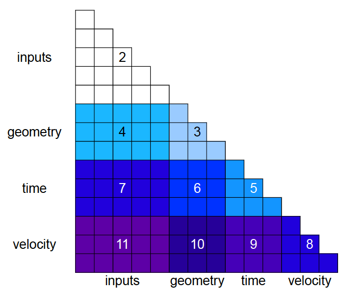
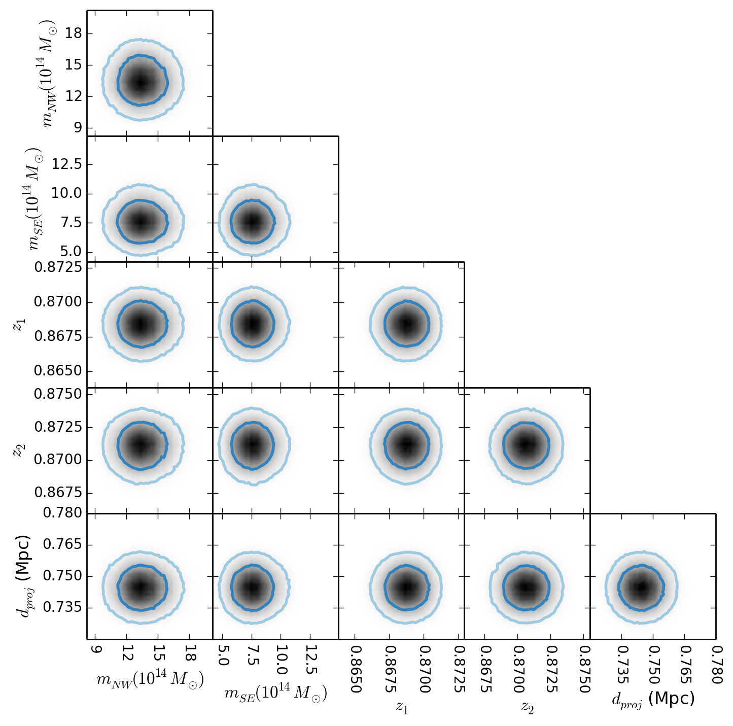
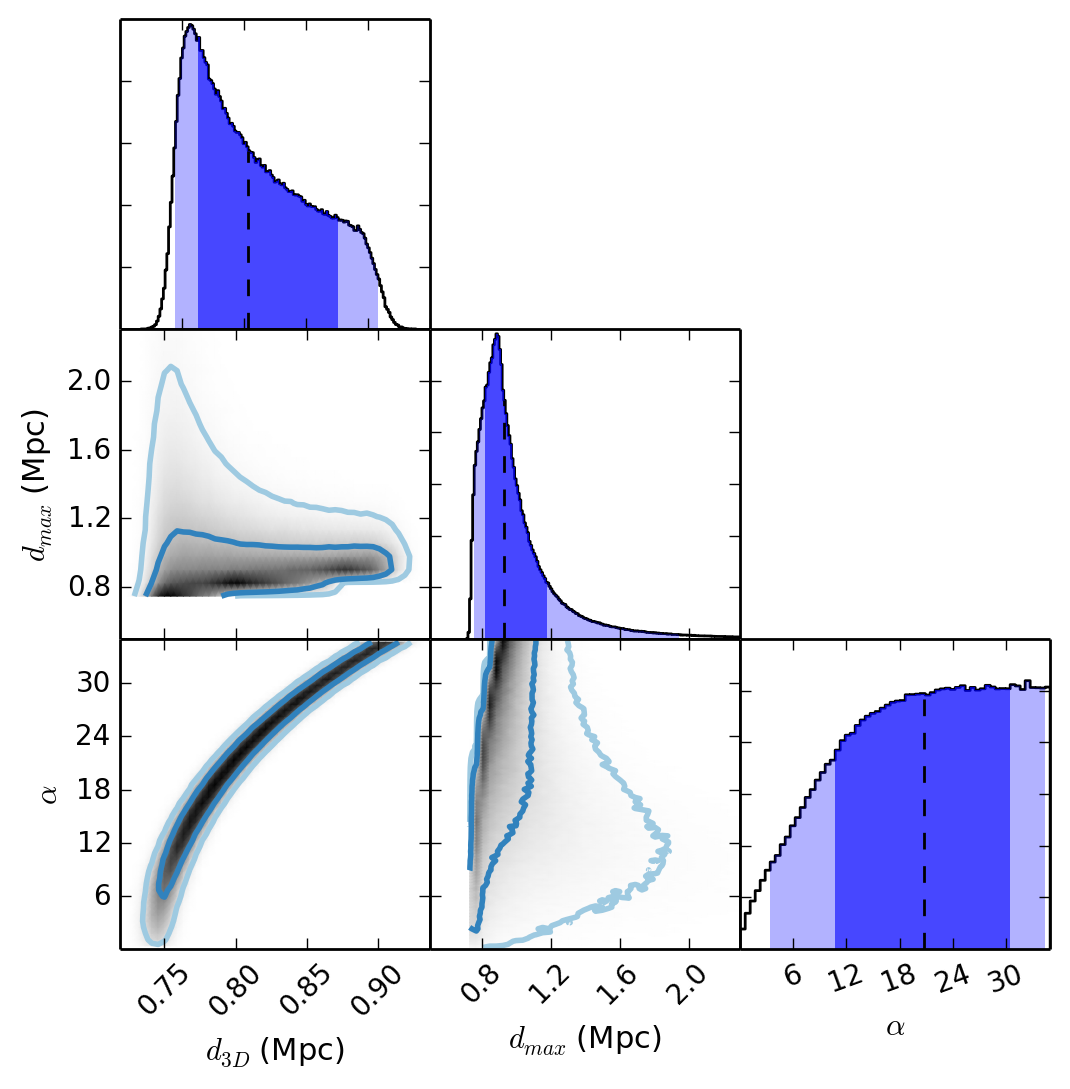
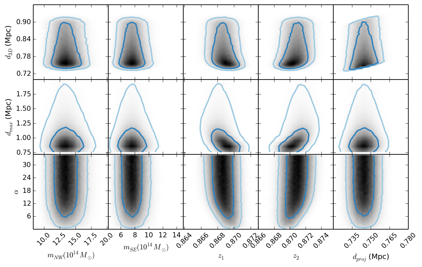
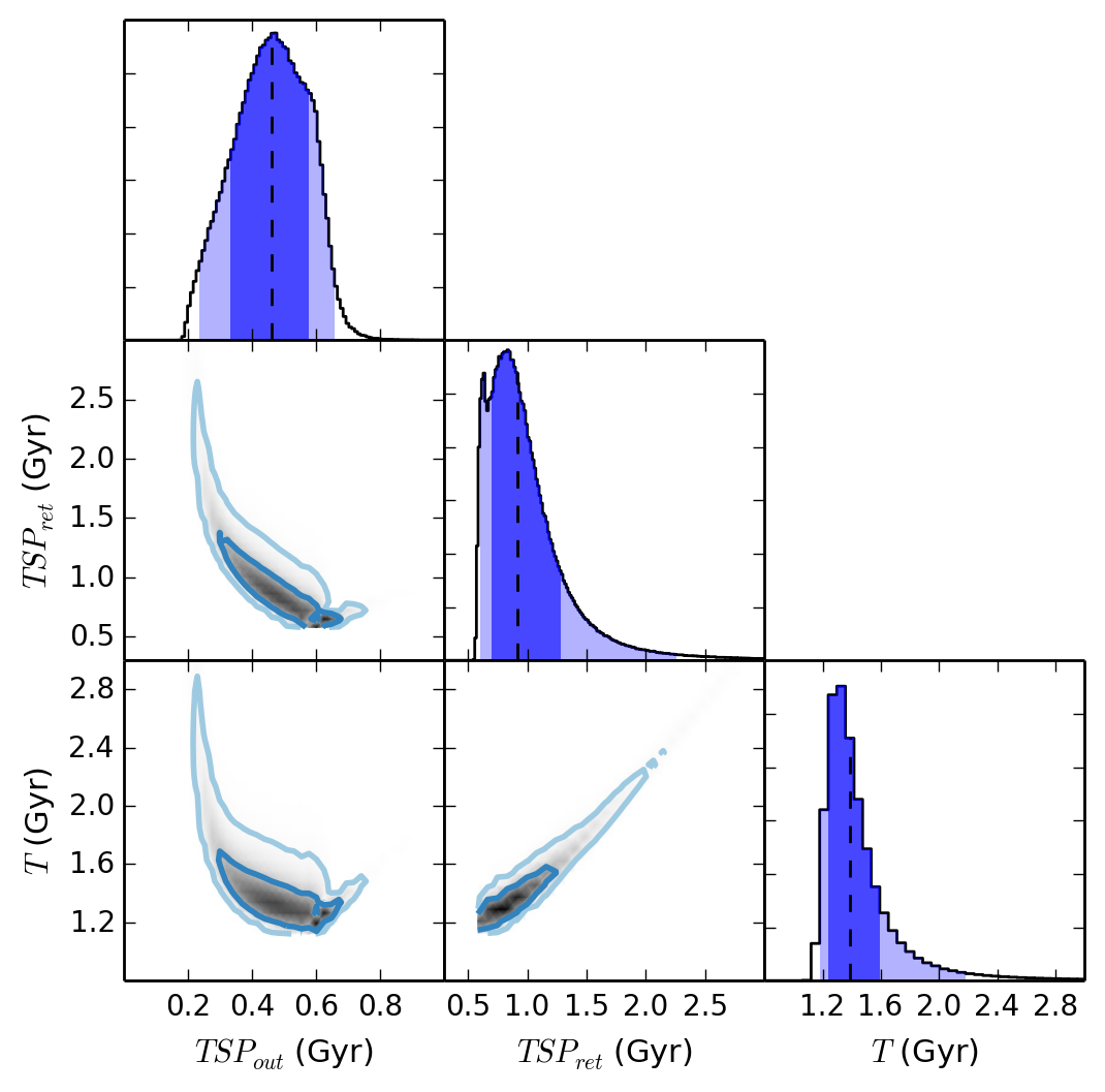
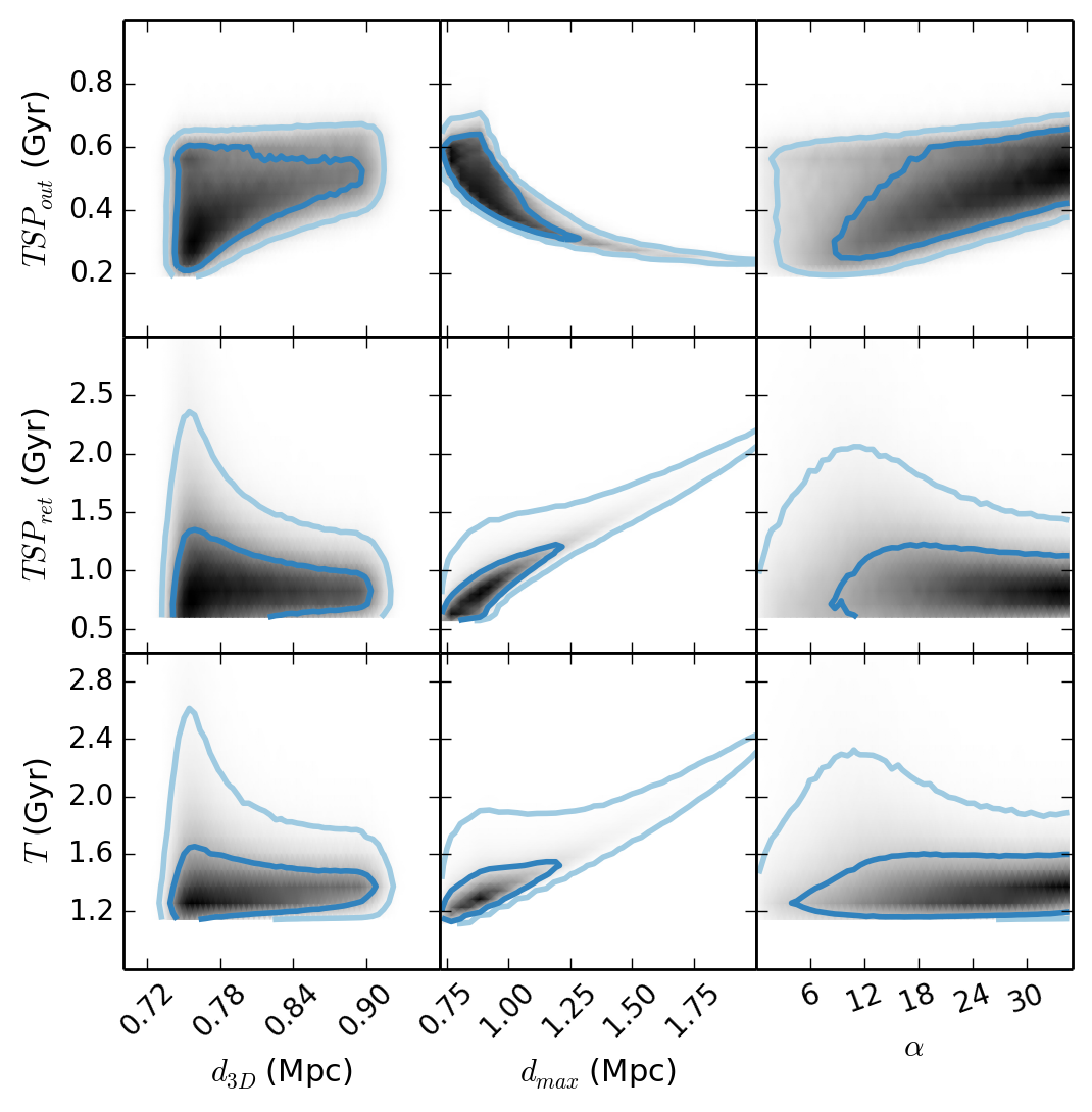
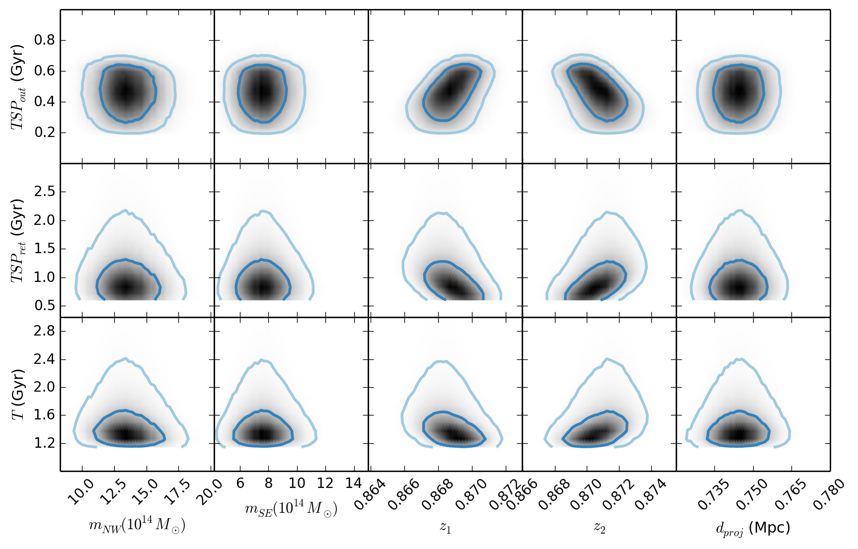
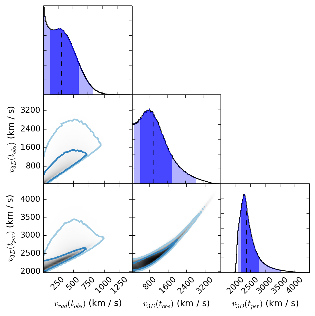
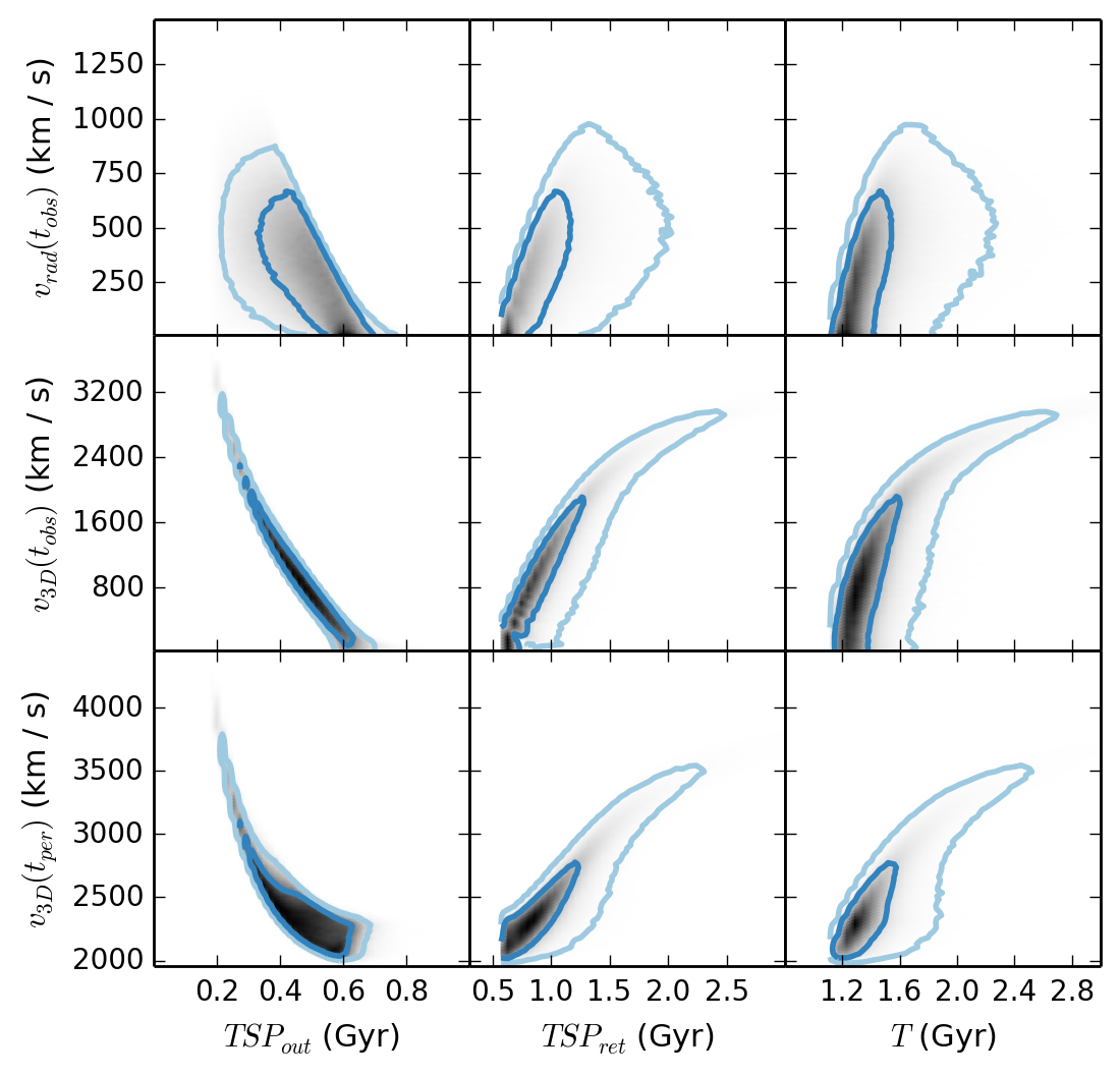
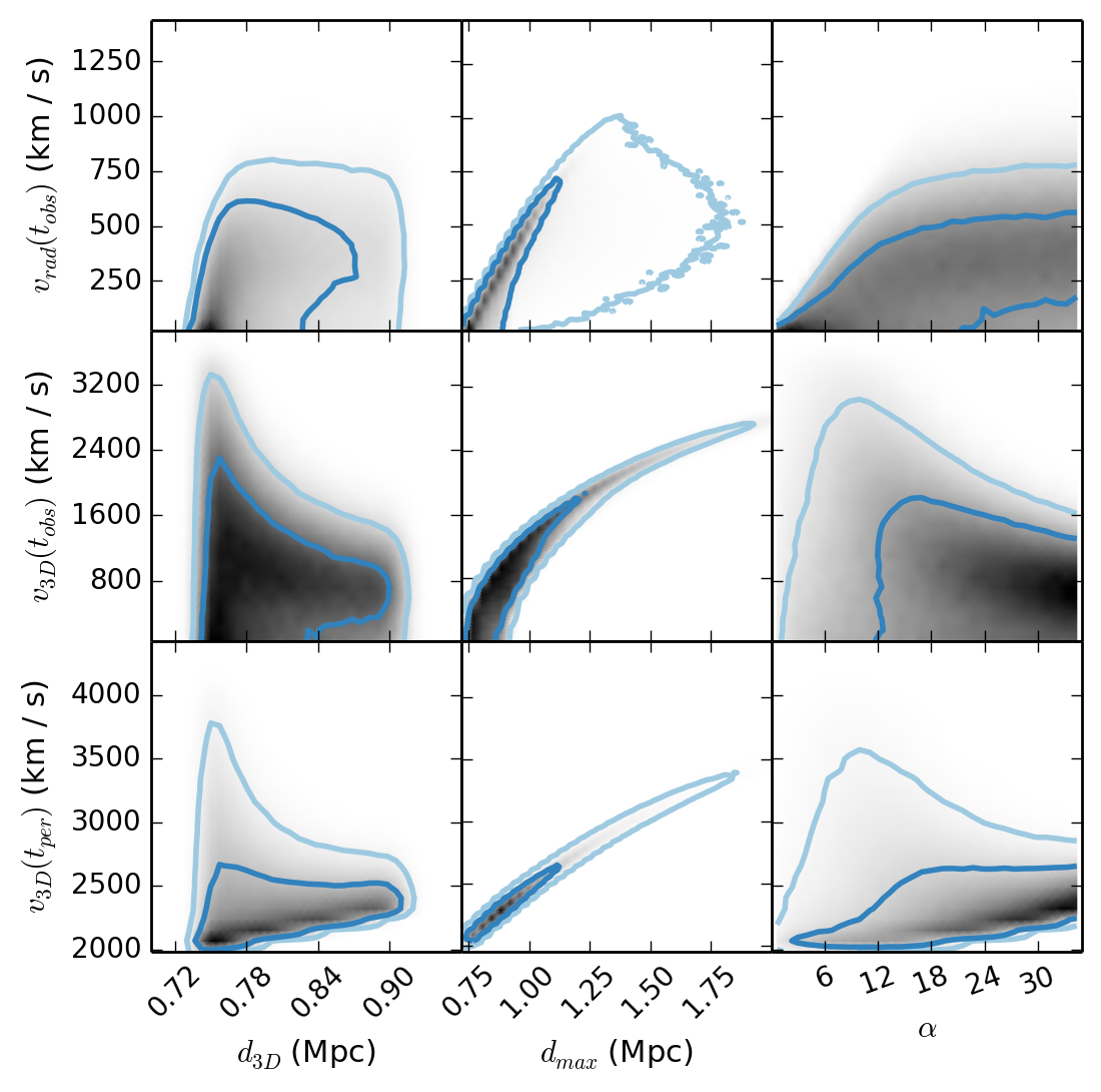
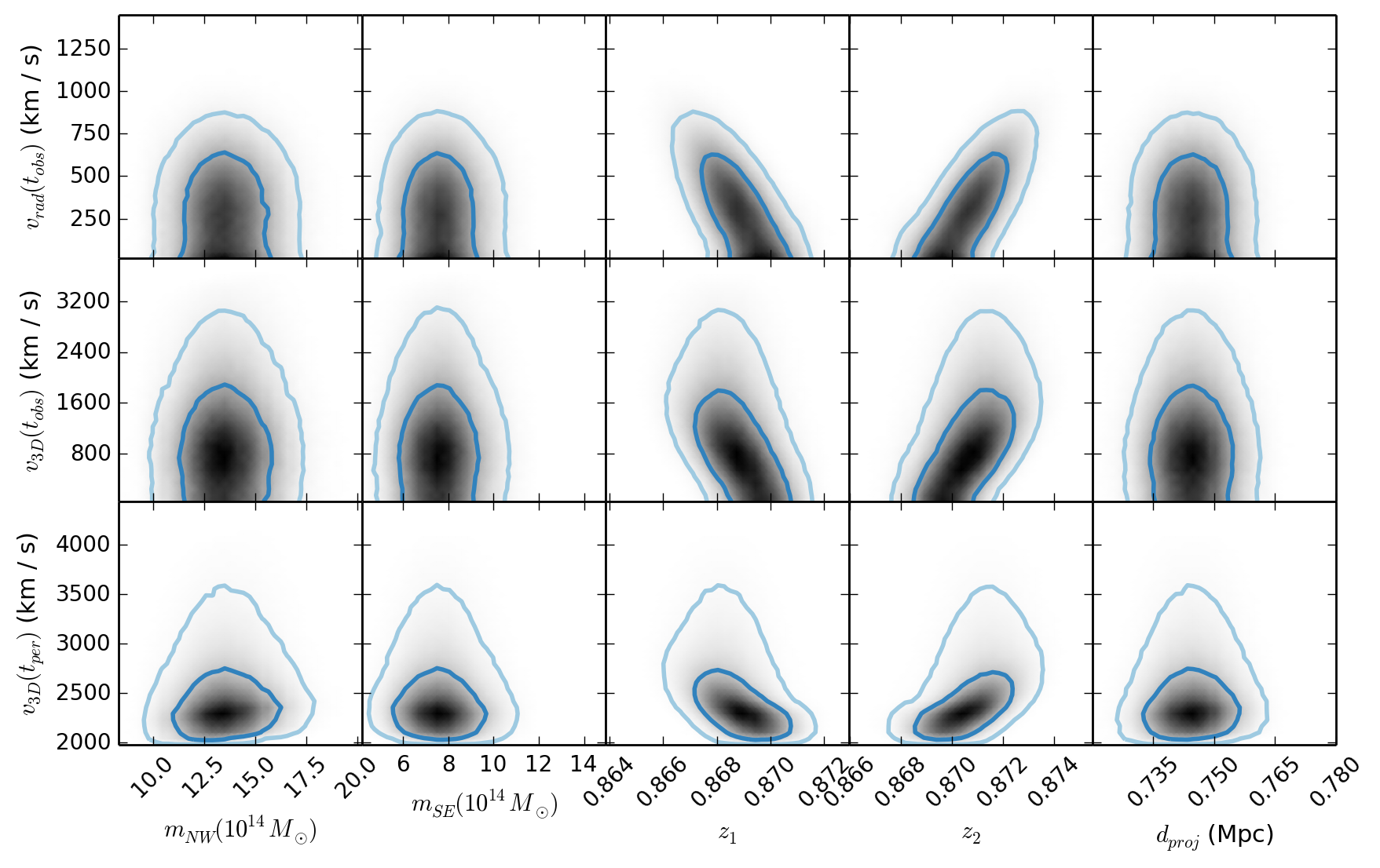
We present the PDFs of the inputs of the dynamical simulation and the marginalized PDFs of the outputs after applying the polarization weight in addition to the default weights. See Fig. 10 for explanations of the order that we present the figures containing the PDFs .

Figure 10: Matrix of variables used in the simulations. We present them in 4 categories, including, inputs, geometry, time and velocity. Regions of the same color represent one plot and the number indicates the corresponding figure number in this appendix.

Figure 11: Marginalized 2-dimensional PDFs of original inputs (vertical axis) and the inputs after applying polarization weight and default weights (horizontal axis). The inner and outer contour denote the central 68% and 95% confidence regions respectively. The circular contours show that the application of weights did not introduce uneven sampling of inputs.

Figure 12: One-dimensional marginalized PDFs (panels on the diagonal) and two-dimensional marginalized PDFs of variables denoting characteristic distances and projection angle of the mergers.

Figure 13: Marginalized PDFs of characteristic distances and projection angle of the merger and the inputs of the simulation.

Figure 14: One-dimensional PDFs of characteristic timescales of the simulation (panels on the diagonal) and the marginalized PDFs of different timescales. Note that there is a default weight for constraining $TSP_{\rm out}$ but not for $TSP_{\rm ret}$ and $T$, so $TSP_{\rm out}$ spans a smaller range.

Figure 15: Marginalized PDFs of characteristic timescales of the simulation and the characteristic distances and the projection angle of the merger.

Figure 16: Marginalized PDFs of characteristic timescales of the simulation and the inputs.

Figure 17: One-dimensional marginalized PDFs of velocities at characteristic times (panels on the diagonal) and marginalized PDFs of different velocities.

Figure 18: Marginalized PDFs velocities and the characteristic timescales of the simulation against the inputs.

Figure 19: Marginalized PDFs of the velocities at characteristic timescales and the characteristic distances and the projection angle of the merger.

Figure 20: Marginalized PDFs of relative velocities characteristic timescales of the simulation and the inputs.

Appendix C COMPARISON OF THE OUTGOING AND RETURNING SCENARIO

Here, we compare the different merger scenarios using the two relics independently and show that they consistently give the conclusion that the returning scenario is favored for the plausible range of $\beta$. For each merger scenario, we compute the (marginalized) probability of producing simulated values ($s_{proj}$) compatible with the observed location of the radio relic ($s_{obs}$).

Quantitatively, we want to compute and compare the probability:

$$P(s_{proj}\text{ compatible with }s_{obs}|M)$$ (15)

$$=\iint f(S_{proj}\cap S_{obs}|M,\beta)f(\beta|M)ds_{proj}d\beta$$ (16)

$$=\iint f(s_{proj}|M,\beta)f(s_{obs})f(\beta|M)ds_{proj}d\beta,$$ (17)

where $f$ indicates the corresponding PDF, $M$ represents one of the merger scenarios, and $\beta$ is defined in equation  8, $s_{proj}\in S_{proj}$ and $s_{obs}\in S_{obs}$. We set our priors set to be uniform for the marginalization:

$$f(\beta|M_{ret})=f(\beta|M_{out})=\begin{cases}&\text{const}~{}\text{if }0.7\leq\beta\leq 1.5\\ &0~{}\text{otherwise}.\end{cases}$$ (18)

which is more conservative than the most likely range of $\beta$, which is $0.7<\beta<1.1$. We found:

$$P(S_{proj}\cap S_{obs}|M_{ret})/P(S_{proj}\cap S_{obs}|M_{out})$$ (19)

$$=\begin{cases}2.1\text{ for the NW relic},\\ 460\text{ for the SE relic},\end{cases}$$ (20)

which shows that the returning scenario is favored over the outgoing scenario.

This test quantity differs from the traditional hypothesis testing or model comparison in several ways:

1. we did not compute a likelihood function. We have adopted non-parametric PDFs in our Monte Carlo simulation,i.e. there is no well-known functional form of the likelihood in our context. We make use of $f(S_{proj}\cap S_{obs})$ to penalize the simulated values being different from our observed data

2. with this quantity, we are not asking whether the expected value of the radio relic such as the mean or median from each model match the observation best. Those estimators take into account the values that do not match the observed location of the radio relic.

3. we marginalized the uncertainty in $\beta$ to be as conservative as possible, instead of assuming a fixed value of $\beta$.

Figure 21: Probability ratio between the returning model (numerator) and the outgoing model at given $\beta$. We remind readers $\beta$ is a factor relating the time-averaged shock velocity and the pericenter velocity of the corresponding subcluster.

Figure 22: Comparison of the PDFs of the observed position of the SE relic (red bar includes 95% confidence interval of location of relic in the center of mass frame) with the predicted position from the two simulated merger scenarios (blue for outgoing and green for the returning scenario). For the plausible values of $\beta<1.1$, the returning scenario is preferred. We obtained similar conclusion about the merger scenario as for the NW relic calculation.

Figure 23: Comparison of the PDFs of the observed position of the NW relic (red bar includes 95% confidence interval of location of relic in the center of mass frame) with the predicted position from the two simulated merger scenarios (blue for outgoing and green for the returning scenario). For the plausible values of $\beta<1.1$, the returning model is preferred. For comparison purpose, we also show that $\beta>1.3$ (top panel) for the outgoing scenario to be favored. Note that we made use of the polarization weight for producing this figure.

References

- Beers et al. (1990) Beers T. C., Flynn K., Gebhardt K., 1990, AJ, 100, 32, doi:10.1086/115487
- Bradač et al. (2006) Bradač M. et al., 2006, ApJ, 652, 937, 0608408, doi:10.1086/508601
- Brüggen et al. (2011) Brüggen M. et al., 2011, Space Sci. Rev., 166, 187, 1107.5223, doi:10.1007/s11214-011-9785-9
- Dawson (2013) Dawson W. a., 2013, ApJ, 772, 131, 1210.0014, doi:10.1088/0004-637X/772/2/131
- Dawson et al. (2012) Dawson W. a. et al., 2012, ApJ, 747, L42, 1110.4391, doi:10.1088/2041-8205/747/2/L42
- Donnert (2014) Donnert J. M. F., 2014, MNRAS, 438, 1971, 1311.7066, doi:10.1093/mnras/stt2291
- Ensslin et al. (1998) Ensslin T. a., Biermann P. L., Klein U., Kohle S., 1998, A&A, 332, 395, 9712293
- Feretti et al. (2012) Feretti L., Giovannini G., Govoni F., Murgia M., 2012, aapr, 20, 54, 1205.1919, doi:10.1007/s00159-012-0054-z
- Hallman & Markevitch (2004) Hallman E. J., Markevitch M., 2004, ApJ, 610, L81, doi:10.1086/423449
- Hasselfield et al. (2013) Hasselfield M. et al., 2013, J. Cosmol. Astropart. Phys., 2013, 008, doi:10.1088/1475-7516/2013/07/008
- Jee et al. (2014) Jee M. J., Hughes J. P., Menanteau F., Sifón C., Mandelbaum R., Barrientos L. F., Infante L., Ng K. Y., 2014, ApJ, 785, 20, 1309.5097, doi:10.1088/0004-637X/785/1/20
- Kahlhoefer et al. (2013) Kahlhoefer F., Schmidt-Hoberg K., Frandsen M. T., Sarkar S., 2013, MNRAS, 437, 2865, 1308.3419, doi:10.1093/mnras/stt2097
- Lage & Farrar (2014) Lage C., Farrar G. R., 2014, arXiv Prepr. arXiv1406.6703, p. 7, 1406.6703, doi:10.1088/1475-7516/2015/02/038
- Lee & Komatsu (2010) Lee J., Komatsu E., 2010, ApJ, 718, 60, doi:10.1088/0004-637X/718/1/60
- Lindner et al. (2014) Lindner R. R. et al., 2014, ApJ, 786, 49, 1310.6786, doi:10.1088/0004-637X/786/1/49
- Markevitch et al. (2004) Markevitch M., Gonzalez A. H., Clowe D., Vikhlinin A., Forman W., Jones C., Murray S., Tucker W., 2004, ApJ, 606, 819, doi:10.1086/383178
- Markevitch & Vikhlinin (2007) Markevitch M., Vikhlinin A., 2007, Phys. Rep., 443, 1, doi:10.1016/j.physrep.2007.01.001
- Marriage et al. (2011) Marriage T. a. et al., 2011, ApJ, 737, 61, doi:10.1088/0004-637X/737/2/61
- Mastropietro & Burkert (2008) Mastropietro C., Burkert A., 2008, MNRAS, 389, 967, doi:10.1111/j.1365-2966.2008.13626.x
- Mathis et al. (2005) Mathis H., Lavaux G., Diego J. M., Silk J., 2005, MNRAS, 357, 801, doi:10.1111/j.1365-2966.2004.08589.x
- Mauch et al. (2003) Mauch T., Murphy T., Buttery H. J., Curran J., Hunstead R. W., Piestrzynski B., Robertson J. G., Sadler E. M., 2003, MNRAS, 342, 1117, doi:10.1046/j.1365-8711.2003.06605.x
- Menanteau et al. (2010) Menanteau F. et al., 2010, ApJ, 723, 1523, doi:10.1088/0004-637X/723/2/1523
- Menanteau et al. (2012) Menanteau F. et al., 2012, ApJ, 748, 7, 1109.0953, doi:10.1088/0004-637X/748/1/7
- Merten et al. (2011) Merten J. et al., 2011, MNRAS, 417, 333, 1103.2772, doi:10.1111/j.1365-2966.2011.19266.x
- Milosavljević et al. (2007) Milosavljević M., Koda J., Nagai D., Nakar E., Shapiro P. R., 2007, ApJ, 661, L131, doi:10.1086/518960
- Molnar & Broadhurst (2015) Molnar S. M., Broadhurst T., 2015, ApJ, 800, 37, 1405.2617, doi:10.1088/0004-637X/800/1/37
- Navarro et al. (1996) Navarro J. F., Frenk C. S., White S. D. M., 1996, ApJ, 462, 563, doi:10.1086/177173
- Paul et al. (2011) Paul S., Iapichino L., Miniati F., Bagchi J., Mannheim K., 2011, ApJ, 726, 17, doi:10.1088/0004-637X/726/1/17
- Perez & Granger (2007) Perez F., Granger B. E., 2007, Comput. Sci. Eng., 9, 21, doi:10.1109/MCSE.2007.53
- Prokhorov & Durret (2007) Prokhorov D. a., Durret F., 2007, A&A, 474, 375, doi:10.1051/0004-6361:20077542
- Randall et al. (2008) Randall S. W., Markevitch M., Clowe D., Gonzalez A. H., Bradač M., Bradac M., 2008, ApJ, 679, 1173, doi:10.1086/587859
- Ricker (1998) Ricker P. M., 1998, ApJ, 496, 670, doi:10.1086/305393
- Robitaille et al. (2013) Robitaille T. P. et al., 2013, A&A, 558, A33, doi:10.1051/0004-6361/201322068
- Sifón et al. (2013) Sifón C. et al., 2013, ApJ, 772, 25, 1201.0991, doi:10.1088/0004-637X/772/1/25
- Skillman et al. (2013) Skillman S. W., Xu H., Hallman E. J., O’Shea B. W., Burns J. O., Li H., Collins D. C., Norman M. L., 2013, ApJ, 765, 21, doi:10.1088/0004-637X/765/1/21
- Springel & Farrar (2007) Springel V., Farrar G. R., 2007, MNRAS, 380, 911, doi:10.1111/j.1365-2966.2007.12159.x
- Stroe et al. (2014) Stroe A., Harwood J. J., Hardcastle M. J., Rottgering H. J. A., 2014, MNRAS, 445, 1213, 1409.1579, doi:10.1093/mnras/stu1839
- Thompson & Nagamine (2012) Thompson R., Nagamine K., 2012, MNRAS, 419, 3560, arXiv:1107.4645v2, doi:10.1111/j.1365-2966.2011.20000.x
- Van Weeren et al. (2011) Van Weeren R. J., Brüggen M., Röttgering H. J. A., Hoeft M., 2011, MNRAS, 418, 230, 1108.1398v1, doi:10.1111/j.1365-2966.2011.19478.x
- van Weeren et al. (2010) van Weeren R. J., Rottgering H. J. A., Bruggen M., Hoeft M., 2010, Science (80-. )., 330, 1, 1010.4306, doi:10.1126/science.1194293
- VanderPlas et al. (2012) VanderPlas J., Connolly A. J., Ivezic Z., Gray A., 2012, in 2012 Conf. Intell. Data Underst.. IEEE, pp 47–54, doi:10.1109/CIDU.2012.6382200
- Vazza et al. (2012) Vazza F. et al., 2012, MNRAS, 421, 1868, 1111.1720, doi:10.1111/j.1365-2966.2011.20160.x
- Zitrin et al. (2013) Zitrin A., Menanteau F., Hughes J. P., Coe D., Barrientos L. F., Infante L., Mandelbaum R., 2013, ApJ, 770, L15, arXiv:1304.0455v1, doi:10.1088/2041-8205/770/1/L15