Abstract

In theory, Bayesian nonparametric (BNP) models are well suited to streaming data scenarios due to their ability to adapt model complexity with the observed data. Unfortunately, such benefits have not been fully realized in practice; existing inference algorithms are either not applicable to streaming applications or not extensible to BNP models. For the special case of Dirichlet processes, streaming inference has been considered. However, there is growing interest in more flexible BNP models building on the class of normalized random measures (NRMs). We work within this general framework and present a streaming variational inference algorithm for NRM mixture models. Our algorithm is based on assumed density filtering (ADF), leading straightforwardly to expectation propagation (EP) for large-scale batch inference as well. We demonstrate the efficacy of the algorithm on clustering documents in large, streaming text corpora.

1 Introduction

Often, data arrive sequentially in time and we are tasked with performing unsupervised learning as the data stream in, without revisiting past data. For example, consider the task of assigning a topic to a news article based on a history of previously assigned documents. The articles arrive daily—or more frequently—with no bound on the total number in the corpus. In clustering such streaming data, Bayesian nonparametric (BNP) models are natural as they allow the number of clusters to grow as data arrive. A challenge, however, is that it is infeasible to store the past cluster assignments, and instead inference algorithms must rely solely on summary statistics of these variables.

Stochastic variational inference (SVI) [1] has become a popular method for scaling posterior inference in Bayesian latent variable models. Although SVI has been extended to BNP models, SVI requires specifying the size of the data set a priori, an inappropriate assumption for streaming data. In contrast, streaming variational Bayes (SVB) [2] handles unbounded data sets by exploiting the sequential nature of Bayes theorem to recursively update an approximation of the posterior. Specifically, the variational approximation of the current posterior becomes the prior when considering new observations. While SVB is appropriate for parametric models, it does not directly generalize to the BNP setting that is essential for streaming data.

For BNP models, streaming inference has been limited to algorithms hand-tailored to specific models. For example, a streaming variational inference algorithm for Dirichlet process (DP) mixture models was recently proposed based on heuristic approximations to the Chinese restaurant process (CRP) predictive distribution associated with the DP [3].

We seek a method for streaming inference in BNP models that is more generally extensible. We are motivated by the recent focus on a broader class of BNP priors—normalized random measures (NRMs)—that enable greater control of various properties than the DP permits. For example, in clustering tasks, there is interest in having flexibility in the distribution of cluster sizes. Throughout the paper, we focus on the specific case of the normalized generalized gamma process (NGGP), though our methods are more general. Recently, NGGP mixture models have been shown to outperform the DP [4, 5], but inference has relied on Markov chain Monte Carlo (MCMC). Due to the limitations of MCMC, such demonstrations have been limited to small data sets. Importantly, NGGPs and the DP differ mainly in their asymptotic scaling properties and the use of NGGPs may be more appropriate in large data sets where the logarithmic cluster growth rate of the DP is not appropriate.

To address the challenge of streaming inference in NRM mixture models, we develop a variational algorithm based on assumed density filtering (ADF) [6]. Our algorithm uses infinite-dimensional approximations to the mixture model posterior and allows general BNP predictive distributions to be used by leveraging an auxiliary variable representation. As a byproduct of the ADF construction, a multi-pass variant straightforwardly yields an expectation propagation (EP) algorithm for batch inference in BNP models. This provides a new approach to scalable BNP batch inference.

In the special case of DPs, our algorithm reduces to that of [3]. As such, our framework forms a theoretically justified and general-purpose scheme for BNP streaming inference, encompassing previous heuristic and model-specific approaches, and with a structure that enables insight into BNP inference via EP.

We demonstrate our algorithm on clustering documents from text corpora using an NRM mixture model based on the NGGP [5]. After a single pass through a modest-sized data set, our streaming variational inference algorithm achieves performance nearly on par with that of a batch sampling-based algorithm that iterates through the data set hundreds of times. We likewise examine a New York Times corpus of 300,000 documents to which the batch algorithm simply does not scale (nor would it be applicable in a truly streaming setting). In these experiments, we justify the importance of considering the flexible class of NRM-based models. Our work represents the first application of non-DP-based NRMs to such large-scale applications.

2 Background

2.1 Completely Random Measures

A completely random measure (CRM) [7] is a distribution over measures $G$ on $\Theta$ such that for disjoint $A_{k}\subset\Theta$, $G(A_{k})$ are independent random variables and

$$G=\sum_{k=1}^{\infty}\pi_{k}\delta_{\theta_{k}}.$$ (1)

The masses $\pi_{k}$ and locations $\theta_{k}$ are characterized by a Poisson process on $\Theta\times\mathbb{R}_{+}$ with Lévy measure $\mu(d\theta,d\pi)$ [7, 8]. We restrict our attention to homogeneous CRMs where $\mu(d\theta,d\pi)=H_{0}(d\theta)\lambda(d\pi)$, a common assumption in the literature  [9, 10, 11]. We denote a draw from a homogeneous CRM as

$$G\sim\mathrm{CRM}(\lambda,H_{0}).$$ (2)

The total mass $T=G(\Theta)=\sum_{k=1}^{\infty}\pi_{k}$ is almost surely finite [12]. However, since $T\neq 1$ in general, CRMs cannot directly be used as priors for mixture models.

2.2 Normalized Random Measures

One can normalize a CRM by its finite total mass to construct a BNP prior for mixture models. Specifically, define the normalized random measure (NRM) $P=\sum_{k=1}^{\infty}\frac{\pi_{k}}{T}\delta_{\theta_{k}}$. The Dirichlet process (DP) is an NRM which arises from normalizing the masses of a gamma process [9]. However, more flexible NRMs can be constructed by starting with different CRMs.

In the mixture model setting, we observe data $\{x_{i}\in\mathbb{R}^{d}\}$ with $x_{i}$ generated from mixture component $\theta^{z_{i}}$. Here, we assume the assignment variables, $z_{i}$, are 1-of-$K$ coded so that $\sum_{k}z_{ik}=1$ and $z_{ik}=1$ implies that observation $i$ is assigned to component $\theta_{k}$ via $\theta^{z_{i}}$. The resulting NRM mixture model can be written as:

$$G\;|\;\lambda,H_{0} \sim\mathrm{CRM}(\lambda,H_{0})$$ (3)

$$z_{i}\;|\;G \sim\sum_{k=1}^{\infty}\frac{\pi_{k}}{T}\delta_{k}$$

$$x_{i}\;|\;z_{i},\theta \sim F(x_{i}|\theta^{z_{i}}),$$

where $F(\cdot|\cdot)$ is an observation model.

For our running example of the normalized generalized gamma process (NGGP), the GGP Lévy measure is

$$\lambda(d\pi)=\frac{a}{\Gamma(1-\sigma)}\pi^{-\sigma-1}e^{-\tau\pi}d\pi,$$ (4)

where $\tau\in[0,\infty)$, $a\in(0,\infty)$, and $\sigma\in[0,1)$. Notable special cases of the NGGP are $\sigma=0$, where we obtain the DP, and $\sigma=0.5$, where we obtain the normalized inverse-Gaussian (IG) process. The NGGP with $\sigma\neq 0$ provides greater control over model properties, such as the distribution of cluster sizes [4].

For any NRM mixture model, by introducing an auxiliary variable $U_{n}\sim\Gamma(n,T)$, we can integrate out the NRM $P$ and define a partial urn scheme [5, 11]. In the case of the NGGP we have:

$$p(z_{{(n+1)}k}|U_{n},z_{1:n}){\propto}\left\{\begin{array}[]{ll}\displaystyle n_{k}-\sigma,\,\,\,\,\,\,\,\,\,\,\,\,\,\,k\leq K\\ a(U_{n}+\tau)^{\sigma},\,\,k=K+1,\end{array}\right.$$ (5)

where $K$ is the number of instantiated clusters in $z_{1:n}$. When $\sigma=0$, Eq. (5) reduces to the well known Chinese restaurant process (CRP) corresponding to the DP. The posterior distribution of $U_{n}$ is given by [11]:

$$p(U_{n}|z_{1:n})\propto\frac{U^{n}_{n}}{(U_{n}+\tau)^{n-aK}}e^{-\frac{a}{\sigma}(U_{n}+\tau)^{\sigma}}.$$ (6)

Together, Eqs. (5) and (6) can be used to define MCMC samplers for NGGP mixture models [5, 13]; our streaming algorithm also exploits the use of $U_{n}$.

2.3 Assumed Density Filtering

Assumed density filtering (ADF) was first developed as a sequential procedure for inference in dynamic models that iteratively projects an intractable distribution onto a simpler family of distributions. Let $z_{1:n}=(z_{1},z_{2},\ldots,z_{n})$ be a sequence of random variables with joint distribution $p_{n}(z_{1:n})$. We can write the joint distribution as a product of factors,

$$p_{n}(z_{1:n})\propto\prod_{i=1}^{n}f_{i}(z_{1:i}).$$ (7)

ADF approximates the sequence of distributions $p_{n}(z_{1:n})$ with a sequence $\hat{q}_{n}(z_{1:n})\in\mathcal{Q}_{n}$, where $\mathcal{Q}_{n}$ is a family of simpler distributions. Based on the current $\hat{q}_{n}(z_{1:n})$, the approximation to $p_{n+1}(z_{1:n+1})$ is formed as follows. The $(n+1)$st factor is incorporated to form $\hat{p}_{n+1}(z_{1:n})\stackrel{{\scriptstyle\triangle}}{{\propto}}f_{n+1}(z_{1:n+1})\hat{q}_{n}(z_{1:n})$, which is then projected onto $\mathcal{Q}_{n+1}$ by minimizing the KL divergence:

$$\hat{q}_{n+1}(z_{1:n+1})=\\ \operatorname*{arg\,min}_{q_{n+1}\in\mathcal{Q}_{n+1}}\mathrm{KL}\Big{(}\hat{p}_{n+1}(z_{1:n+1})||q_{n+1}(z_{1:n+1})\Big{)}.$$ (8)

When $\mathcal{Q}_{n}$ factorizes as $q_{n}(z_{1:n})=\prod_{i=1}^{n}q_{n}(z_{i})$, the optimal distribution for each factor is given by the marginal distribution, $\hat{q}_{n+1}(z_{i})\propto\int f_{n+1}(z_{1:n+1})\hat{q}_{n}(z_{1:n})dz_{\backslash i}$, where $z_{\backslash i}$ denotes the set $\{z_{j},j\neq i\}$. The tractability of this integral for certain families of factors $f_{n}$ and $\hat{q}_{n}$ motivates ADF, and in particular, the recursive projection onto $\{\mathcal{Q}_{n}\}$.

2.4 Expectation Propagation

ADF can be generalized to perform batch inference in static models resulting in the well known expectation propagation (EP) algorithm [6]. In EP, one approximates an intractable, factorized distribution over a fixed set of model parameters, $\theta$, with a tractable distribution, $q\in\mathcal{Q}$. In place of Eq. (7), we have

$$p(\theta)\propto\prod_{i=1}^{n}f_{i}(\theta).$$ (9)

An EP iteration begins with both a posterior approximation, $\hat{q}(\theta)$, and stored local contributions, $\bar{q}_{j}(\theta)$, associated with each factor $f_{j}(\theta)$. To refine the posterior approximation, a local contribution is removed to form a normalized approximation to the remaining $n-1$ factors, $\hat{q}_{\setminus j}(\theta)\propto\frac{q_{\theta)}}{\bar{q}_{j}(\theta)}$. As in ADF, the $j$th factor is then appended to the approximation $\hat{q}_{\setminus j}$ and projected back onto $\mathcal{Q}$ to obtain a refined $\hat{q}(\theta)$:

$$\hat{q}(\theta)=\operatorname*{arg\,min}_{q\in\mathcal{Q}}\mathrm{KL}\Big{(}\hat{p}(\theta)\propto f_{j}(\theta)\hat{q}_{\setminus j}(\theta)\Big{|}\Big{|}q(\theta)\Big{)}.$$ (10)

The $j$th local contribution is then updated to

$$\bar{q}_{j}(\theta)\propto\frac{\hat{q}(\theta)}{\hat{q}_{\setminus j}(\theta)}.$$ (11)

When $\hat{q},\bar{q}_{j},\hat{q}_{\setminus j}$ are in the exponential family with the same type of sufficient statistics, $\hat{\nu},\bar{\nu}_{j},\hat{\nu}_{\setminus j}\in\mathbb{R}^{m}$, respectively, then $\bar{\nu}_{j}=\hat{\nu}-\hat{\nu}_{\setminus j}$. This process of removing local statistics from the approximation, adding in the respective factor, and re-projecting onto $\mathcal{Q}$ is repeated for all factors until convergence.

The link between ADF and EP, comparing Eqs. (8) and (10), allows us to extend our streaming BNP algorithm of Sec. 3 to EP for batch inference (Sec. 3.4). EP is easily parallelized [14], allowing these methods to scale to massive batch data sets, though we leave the parallel extension of our method to future work.

3 Streaming Variational Inference for BNP Mixture Models

We now turn to deriving a streaming inference algorithm for the NRM mixture model of Eq. (3). Here, our goal is joint inference of the growing set of local cluster indicators, $z_{1:n}$, and the static set of global cluster parameters, $\theta=\{\theta_{k}\}_{k=1}^{\infty}$. The method is derived from the ADF algorithm of Sec. 2.3 and boils down to: (1) a local update of cluster soft assignments for the current data point and (2) a global update of cluster variational parameters. The local update follows directly from ADF. Embedded in this step is computing the NRM predictive probability on cluster assignments, for which we use the auxiliary variable representation of Eq. (5) combined with an additional variational approximation to compute an intractable integral. For computational tractability, the global step uses an approximation similar to that proposed in [15], though an exact ADF update is possible.

To start, note that the posterior for the first $n$ assignments, $z_{1:n}$, and cluster parameters, $\theta$, factorizes as:

$$p_{n}(z_{1:n},\theta|x_{1:n}) \propto p(x_{n}|z_{n},\theta)p(z_{n}|z_{1:n-1})$$ (12)

$$\hskip 1.00006pt\times p(z_{1:n-1},\theta|x_{1:n-1})$$

$$\propto p(\theta)\prod_{i=1}^{n}p(x_{i}|z_{i},\theta)p(z_{i}|z_{1:i-1}).$$ (13)

Eq. (12) emphasizes the sequential decomposition of the posterior while Eq. (13) concretely links our derivation with ADF. We set the first factor to $p(x_{1}|z_{1},\theta)p(z_{1})\prod_{k=1}^{\infty}p(\theta_{k})$, where $p(z_{11}=1)=1$ so that $p(x_{1}|z_{1},\theta)p(z_{1})=p(x_{1}|\theta_{1})p(z_{1})$. For $i>1$, we define $p(z_{i}|z_{1:i-1})$ as the $i$th predictive factor and $p(x_{i}|z_{i},\theta)$ as the $i$th likelihood factor. We then apply ADF to this sequence of factors in Eq. (13) to obtain a sequence of factorized variational approximations of the form $\hat{q}_{n}(z_{1:n},\theta)=\prod_{k=1}^{\infty}\hat{q}_{n}(\theta_{k})\prod_{i=1}^{n}\hat{q}_{n}(z_{i})$. Since the first factor takes this factorized form, we have $\hat{q}_{1}(z_{1},\theta)\propto p(z_{1})p(x_{1}|\theta_{1})p(\theta_{1})\prod_{k=2}^{\infty}p(\theta_{k})$; algorithmically we only update $\hat{q}_{1}(z_{1})$ and $\hat{q}_{1}(\theta_{1})$. For subsequent factors, assume the posterior $p(z_{1:n-1},\theta|x_{1:n-1})$ is approximated by a factorized $\hat{q}_{n-1}(z_{1:n-1},\theta)$. For $n>2$, we add $p(z_{n}|z_{1:n-1})$, perform an ADF step, and then add $p(x_{n}|z_{n},\theta)$ and perform another ADF step.

Predictive factors

To approximate the posterior after adding the $p(z_{n}|z_{1:n-1})$ factor, we use Eq. (8):

$$q^{\mathrm{pr}}(z_{1:n},\theta)=\operatorname*{arg\,min}_{q_{n}\in\mathcal{Q}_{n}}\mathrm{KL}\Big{(}\hat{p}_{n}(z_{1:n},\theta|x_{1:n-1})||q_{n}(z_{1:n},\theta)\Big{)}.$$

where $\hat{p}_{n}(z_{1:n},\theta|x_{1:n-1})\stackrel{{\scriptstyle\triangle}}{{\propto}}p(z_{n}|z_{1:n-1})\hat{q}_{n-1}(z_{1:n-1},\theta)$ is the propagated variational distribution and $q^{\mathrm{pr}}$ its projection back to $Q_{n}$. For $i<n$, the optimal approximation for the local variables, $z_{i}$, is $q^{\mathrm{pr}}(z_{i})=\hat{q}_{n-1}(z_{i})$, while for the $n$th local variable we have

$$q^{\mathrm{pr}}(z_{n})=\sum_{z_{1:n-1}}p(z_{n}|z_{1:n-1})\prod_{i=1}^{n-1}\hat{q}_{n-1}(z_{i}).$$ (14)

The combinatorial sum over $z_{1:n-1}$ embedded in evaluating $q^{\mathrm{pr}}(z_{n})$ appears to be a daunting barrier to efficient streaming inference. However, as we show in Sec. 3.1, for the models we consider the resulting $q^{\mathrm{pr}}$ can be written in terms of sums of local soft assignments, $\sum_{i=1}^{n-1}\hat{q}_{n-1}(z_{i})$. Since these past soft assignments remain unchanged, the sum—instead of past assignment histories—can be stored as a sufficient statistic. Furthermore, since $p(z_{n}|z_{1:n-1})$ places mass on $z_{n}$ taking a previously unseen component, the approximation $q^{\mathrm{pr}}(z_{n})$ inherits this ability and allows our algorithm to introduce new components when needed. This is a crucial feature of our approach that enables our approximate inference scheme to maintain the benefits of nonparametric modeling, and is in contrast to approaches based on truncations to the underlying NRM or on heuristics for creating new clusters.

Since the predictive factor does not depend on $\theta$, the approximation for $\theta$ is retained: $q^{\mathrm{pr}}(\theta_{j})=\hat{q}_{n-1}(\theta_{j})$.

Likelihood factors

We apply Eq. (8) to obtain the approximation after adding the $p(x_{n}|z_{n},\theta)$ factor

$$\hat{q}_{n}(z_{1:n},\theta)=\operatorname*{arg\,min}_{q_{n}\in\mathcal{Q}_{n}}\mathrm{KL}\Big{(}\hat{p}_{n}(z_{1:n},\theta|x_{1:n})||q_{n}(z_{1:n},\theta)\Big{)},$$

where $\hat{p}_{n}(z_{1:n},\theta|x_{1:n})\stackrel{{\scriptstyle\triangle}}{{\propto}}p(x_{n}|z_{n},\theta)q^{\mathrm{pr}}(z_{1:n},\theta)$ is the updated variational distribution. Projecting back to $Q_{n}$, for $i<n$ the optimal distributions for the $z_{i}$ are retained: $\hat{q}_{n}(z_{i})=\hat{q}_{n-1}(z_{i})$. For $z_{n}$, we have

$$\hat{q}_{n}(z_{nk}) \propto q^{\mathrm{pr}}(z_{nk})\int p(x_{n}|z_{nk},\theta)\hat{q}_{n-1}(\theta_{k})d\theta_{k},$$ (15)

where $q^{\mathrm{pr}}(z_{nk})$ mirrors the role of the predictive rule, $p(z_{n}|z_{1:n-1})$, when assignments are fully observed. We consider conjugate exponential family models so that $\hat{q}_{n-1}(\theta_{k})$ is in the same family as $p(\theta_{k})$, allowing the integral in Eq. (15) to be given in closed form.

The update in Eq. (15) has appeared previously in both batch [15] and streaming [3] inference algorithms for DP mixtures (without being derived from the ADF framework). In the batch case, $q^{\mathrm{pr}}(z_{n})$ was evaluated by sampling, and in the latter case a heuristic approximation was used. We instead use a principled variational approximation to evaluate Eq. (15), which extends to a large class of NRMs. See Sec. 3.1.

As in EP [6], the optimal update for the global parameters, $\theta_{k}$, after addition of the likelihood factor is proportional to the marginal:

$$\hat{q}_{n}(\theta_{k})\propto\sum_{z_{1:n}}\int p(x_{n}|z_{n},\theta)q^{\mathrm{pr}}(z_{1:n},\theta)d\theta_{\backslash k}.$$ (16)

Eq. (16) is often intractable so we use the conjugate variational Bayes update for $\theta_{k}$ as in [15], giving:

$$\log\hat{q}_{n}(\theta_{k}) \approx\mathbb{E}_{\theta_{\backslash k},z_{n}}\log[p(x_{n}|z_{n},\theta)\hat{q}_{n-1}(\theta)]+C,$$ (17)

where $C$ is a constant. See the Supplement for details. The expectation is with respect to the distributions $\hat{q}_{n}(z_{n})$ and $\hat{q}_{n}(\theta_{\backslash k})=\prod_{j\neq k}\hat{q}_{n}(\theta_{j})$. This implies that

$$\log\hat{q}_{n}(\theta_{k})\approx\hat{q}_{n}(z_{nk})\log p(x_{n}|z_{nk},\theta)+\log\hat{q}_{n-1}(\theta_{k})+C^{\prime}.$$ (18)

For the conjugate models we consider, Eq. (18) leads to tractable updates. Our streaming algorithm, which we refer to as ADF-NRM, proceeds at each step by first computing the local update in Eq. (15), and then the global update in Eq. (18). See Alg. 1.

3.1 Predictive Rule for NGGPs

A key part of the streaming algorithm is efficiently computing $q^{\mathrm{pr}}(z_{n})$. When a DP prior is used, $q^{\mathrm{pr}}(z_{n})$ admits a simple form similar to the CRP:

$$q^{\mathrm{pr}}(z_{nk}){\propto}\left\{\begin{array}[]{ll}\displaystyle\sum_{i=1}^{n-1}\hat{q}_{i}(z_{ik}),&k\leq K_{n-1}\\ a,&k=K_{n-1}+1,\end{array}\right.$$ (19)

where $K_{n-1}$ is the number of considered components in $x_{1:n-1}$ (see Sec. 3.3). Unfortunately, NRMs do not admit such a straightforward expression for $q^{\mathrm{pr}}(z_{n})$ since in general $p(z_{n}|z_{1:n-1})$ is not known in closed form and for NGGPs it is given by a computationally demanding and numerically unstable expression [16] unsuitable for large, streaming data.

Instead, as in Eq. (5), we can introduce an auxiliary variable, $U_{n}$, to obtain a tractable variational approximation for NRMs, as detailed in the Supplement. We focus on the popular case of the NGGP here.

We rewrite $q^{\mathrm{pr}}(z_{n})$ in terms of $U_{n-1}$ and the unnormalized masses, $\pi$, and integrate over these variables:

$$q^{\mathrm{pr}}(z_{n})= \sum_{z_{1:n-1}}\iint\Bigg{[}p(z_{n}|\pi)p(\pi|U_{n-1},z_{1:n-1})$$ (20)

$$\times p(U_{n-1}|z_{1:n-1})\prod_{i=1}^{n-1}\hat{q}_{n-1}(z_{i})\Bigg{]}dU_{n-1}d\pi.$$

The term $p(\pi|U_{n},z_{1:n-1})$ is stated in the Supplement and $p(U_{n-1}|z_{1:n-1})$ is shown in Eq. (6). The random measure $\pi$ consists of a set of instantiated atoms, $\pi_{1},\ldots,\pi_{K}$, and a Poisson process $\pi^{*}$ representing the remaining mass. Since the integral in Eq. (2.1) is intractable, we introduce a partially factorized approximation: $p(\pi|U_{n-1},z_{1:n-1})p(U_{n-1}|z_{1:n-1})\approx q(\pi|U_{n-1})q(U_{n-1})\in\mathcal{Q}_{\pi\times U}$ and solve

$$\operatorname*{arg\,min}_{q\in\mathcal{Q}_{\pi\times U}}\mathrm{KL}\Big{(} q(\pi|U_{n-1})q(U_{n-1})\hat{q}(z_{1:n-1})||$$

$$p(\pi|U_{n-1},z_{1:n-1})p(U_{n-1}|z_{1:n-1})\hat{q}(z_{1:n-1})\Big{)}.$$

The optimal distributions are given by:

$$q(U_{n-1}) \propto e^{-\frac{a}{\sigma}(U_{n-1}+\tau)^{\sigma}}\frac{U^{n-1}_{n-1}}{(U_{n-1}+\tau)^{n-1-a\mathbb{E}_{\hat{q}}[K_{n-1}]}}$$ (21)

$$q(\pi_{k}|U_{n-1}) \propto\pi_{k}^{\mathbb{E}_{\hat{q}}[n_{k}]}e^{-U_{n-1}\pi_{k}}\lambda(d\pi_{k}),$$ (22)

where $\mathbb{E}_{\hat{q}_{n-1}}[K_{n-1}]$ is the expected number of clusters observed so far, which can be recursively computed as described in the Supplement, and $\mathbb{E}_{\hat{q}_{n-1}}[n_{k}]=\sum_{i=1}^{n-1}\hat{q}_{n-1}(z_{ik})$ is the expected number of assignments to component $k$. The variational distribution of $\pi^{*}$ is a Poisson process with tilted Lévy measure $e^{U_{n-1}\pi}\lambda(d\pi)$. As detailed in the Supplement, using these variational approximations in Eq. (2.1) combined with a delta function approximation to $q(U_{m-1})$ yields:

$$q^{\mathrm{pr}}(z_{nk}){\propto}\left\{\begin{array}[]{ll}\displaystyle\max\left(\sum_{i=1}^{n-1}\hat{q}_{i}(z_{ik})-\sigma,0\right),k\leq K_{n-1}\\ a(\hat{U}_{n-1}+\tau)^{\sigma},\,\,\,\,\,\,\,\,\,\,\,\,\,\,\,\,\,\,\,\ k=K_{n-1}+1,\end{array}\right.$$ (23)

where $\hat{U}_{n-1}=\operatorname*{arg\,max}q(U_{n-1})$. For the DP ($\sigma=0$), Eq. (23) reduces to Eq. (19) and the resulting algorithm reduces to that of [3]. Note the differences between Eqs. (23) and (5) and between Eqs. (21) and (6). In both cases, hard assignments are replaced by soft assignments. As previously noted, the sum of these past soft assignments serve as sufficient statistics, and since they do not change between iterations, can be stored in place of individual assignments. Furthermore, the recursive computation of $\mathbb{E}_{\hat{q}_{n-1}}[K_{n-1}]$ in Eq. (21) allows past assignments to be discarded.

  Initialize: $K=1,S_{1}=1$

  $\hat{q}_{1}(\theta_{1})\propto p(x_{1}|\theta_{1})p(\theta_{1})$, $\hat{q}_{1}(z_{11})=1$

  for $n=1$ to $\infty$  do

     $\hat{U}_{n}=\operatorname*{arg\,max}q(U_{n})\mbox{ with $q(U_{n})$ in Eq. \eqref{eqn:u_var}}$

     for $k=1$ to K do

        $q^{\mathrm{pr}}(z_{nk})\propto\max(S_{k}-\sigma,0)$

        $\hat{q}_{n}(z_{nk})\propto q^{\mathrm{pr}}(z_{nk})\int p(x_{n}|z_{nk},\theta_{k})\hat{q}_{n-1}(\theta_{k})d\theta_{k}$

     end for

     $q^{\mathrm{pr}}(z_{n,K+1})\propto a(\hat{U}_{n}+\tau)^{\sigma}$

     $\hat{q}_{n}(z_{n,K+1})\propto q^{\mathrm{pr}}(z_{n,K+1})$

     $\,\,\,\,\,\,\,\,\,\,\,\,\,\,\,\,\,\,\,\,\,\,\,\,\,\,\,\,\,\,\,\,\,\,\,\,\,\,\,\,\,\,\,\times\int p(x_{n}|z_{n,K+1},\theta)p(\theta_{K+1})d\theta_{K+1}$

     normalize $\hat{q}_{n}(z_{n,1:K+1})$

     if $\hat{q}_{n}(z_{n,K+1})>\epsilon$ then

        $S_{K+1}=0$, $\hat{q}_{n-1}(\theta_{K+1})=p(\theta_{K+1}),K=K+1$

     else

        normalize $\hat{q}_{n}(z_{n,1:K})$

     end if

     for $k=1$ to $K$ do

        $\hat{q}_{n}(\theta_{k})\propto p(x_{n}|z_{nk},\theta_{k})^{\hat{q}_{n}(z_{nk})}\hat{q}_{n-1}(\theta_{k})$

        $S_{k}=S_{k}+\hat{q}_{n}(z_{nk})$

     end for

  end for

Algorithm 1 ADF for NRM mixture models

3.2 Computational Complexity

Due to the streaming nature of the ADF-NRM algorithm, we analyze the per-observation complexity. As seen in Alg. 1, for each observation we compute a finite dimensional probability vector with $K_{n}+1$ elements, which is $O(K_{n})$. Additionally, we need to compute $\hat{U}_{n}$ via numerical optimization of $q(U_{n})$, which is a univariate and unimodal function so can be maximized efficiently with complexity denoted $O(\mathcal{U})$. Thus, the per-iteration complexity of ADF-NRM is $O(K_{n}+\mathcal{U})$. In practice the runtime is dominated by the $O(K_{n})$ term due to the NGGP introducing many clusters; the optimization of $\hat{U}_{n}$ terminates in a few iterations (independent of $K_{n}$) and so does not limit the scalability. It is known that $\mathbb{E}[K_{n}]\simeq a\log n$ for the DP and follows a power-law with index $\sigma\in(0,1)$ for the NGGP [17]. This implies that for large $n$ the complexity of ADF-NRM with a NGGP is larger than that with a DP, but is sub-linear in $n$, remaing computationally feasible. Of course, a posteriori $K_{n}$ can grow much more slowly when the data has a compact representation.

3.3 Efficiently Coping with New Clusters

While the probability that a data point belongs to a new cluster, $\hat{q}_{n}(z_{n,K+1})$, is always greater than zero, it is computationally infeasible to introduce a new component at each iteration since the per iteration complexity of ADF-NRM is $O(K_{n})$. In practice, new components are added only if $\hat{q}_{n}(z_{n,K_{n}+1})>\epsilon$ for $\epsilon\geq\sigma$ a threshold. The restriction $\epsilon\geq\sigma$ is natural: if $\hat{q}_{n}(z_{n,K_{n}+1})<\sigma$ then $K_{n}+1$ will be assigned zero prior probability at step $n+1$ in Eq. (23) and will be effectively removed. The threshold parameter explicitly controls the trade off between accuracy and speed; a larger threshold introduces fewer clusters leading to a worse variational approximation but faster run times. One can view our thresholding as an adaptive truncation of the posterior, in contrast to the common approach of truncating the component prior.

During execution of ADF-NRM and EP-NRM of Sec. 3.4, redundant clusters can be created due to the order of observations processed. As in [3], we introduce merge steps to combine distinct clusters that explain similar observations. Since a benefit of the NGGP over the DP is the addition of many small but important clusters (see Sec. 4), we found that frequent merging degrades predictive performance of NGGP models by prematurely removing these clusters. In our experiments, we only merge clusters whose similarity exceeds a conservatively large merge threshold.

3.4 Extension to EP

For data sets of fixed size, $N$, ADF-NRM can be extended to EP-NRM for batch inference analogously to Sec. 2.4. Assume we have both an approximation to the batch posterior $\hat{q}(\theta,z_{1:N})$ and local contributions $\bar{q}_{j}(\theta,z_{j})$ for $j=1,\dots,N$, both of which can be computed using ADF. In particular, $\hat{q}(\theta,z_{1:N})=\hat{q}_{N}(\theta,z_{1:N})$, the final ADF posterior approximation, and $\bar{q}_{j}(\theta,z_{j})\propto\frac{\hat{q}_{j}(\theta,z_{1:j})}{\hat{q}_{j-1}(\theta,z_{1:(j-1)})}$, the ratio between successive ADF approximations. Now define

$$\hat{q}_{\backslash j}(\theta,z_{\setminus j})\propto\frac{\hat{q}(\theta,z_{1:N})}{\bar{q}_{j}(\theta,z_{j})}$$ (24)

to be the approximate posterior with $x_{j}$ removed. We refine $\hat{q}(\theta,z_{1:N})$ using the two step approach outlined in Section 3, first appending the predictive factor, $p(z_{j}|z_{\setminus j})$, to $\hat{q}_{\backslash j}(\theta,z_{\setminus j})$, followed by a projection step, and then adding the likelihood factor, $p(x_{j}|z_{j},\theta)$, again followed by a projection step. Similar to ADF, the updated soft assignment for $z_{j}$ is given by $\hat{q}(z_{jk})\propto q^{\mathrm{pr}}_{\setminus j}(z_{jk})\int p(x_{j}|z_{jk},\theta)\hat{q}_{\setminus j}(\theta_{k})d\theta_{k}$ where $q^{\mathrm{pr}}_{\setminus j}$ is the approximate predictive distribution given all other soft assignments. The global update is given by $\hat{q}(\theta_{k})\propto p(x_{j}|z_{jk},\theta)^{\hat{q}(z_{jk})}\hat{q}_{\setminus j}(\theta_{k})$. The $j$th local contribution is

$$\bar{q}_{j}(\theta,z_{j})\propto\frac{\hat{q}(\theta,z_{1:N})}{\hat{q}_{\backslash j}(\theta,z_{\backslash j})}.$$ (25)

We cycle through the data set repeatedly, applying the steps above, until convergence.

For conjugate exponential families, the computations required for the global cluster parameters, $\theta$, in Eq. (24) and Eq. (25) reduce to updating sufficient statistics as in Sec. 2.4. $q^{\mathrm{pr}}_{\setminus j}$ for NGGPs may similarly be updated on each round by letting $S_{k}=\sum_{i=1}^{N}\hat{q}(z_{ik})$ and $S_{k,\setminus j}=S_{k}-\hat{q}(z_{jk})$, where $\hat{q}(z_{ik})$ are the current soft assignments. Under the same logic as Eq. (23), $q^{\mathrm{pr}}_{\setminus j}$ for instantiated clusters is approximated by

$$q^{\mathrm{pr}}_{\backslash j}(z_{jk}) \propto\max(S_{k,\setminus j}-\sigma,0),$$ (26)

and $q^{\mathrm{pr}}_{\backslash j}(z_{j,K+1})$ follows analogously (see Supplement). After computing the refined soft assignment, $\hat{q}(z_{jk})$, we update $S_{k}=S_{k,\setminus j}+\hat{q}(z_{jk})$. As a consequence of this approach, the total weight on an instantiated cluster $k$, $S_{k}$, can become small upon revisits of the data assignments. In practice, we remove cluster $k$ if $S_{k}<\epsilon$, where $\epsilon$ is as in Sec. 3.3.

4 Experiments

We evaluate ADF-NRM on both real and synthetic data using the task of document clustering. Each document is represented by a vector of word counts, $x_{d}\in\mathbb{R}_{+}^{V}$, where $V$ is the size of the vocabulary, and $x_{dw}$ is the number of occurrences of word $w$ in document $d$. We then model the corpus as a NGGP mixture of multinomials; that is, our data are generated as in Eq. (3) with $x_{d}\sim\mathrm{Mult}(N_{d},\theta^{z_{d}})$, where $N_{d}$ is the number of words in document $d$ and $\theta_{k}$ is a vector of word probabilities in cluster $k$. We take $H_{0}$ to be Dirichlet such that $\theta_{k}\sim\mathrm{Dir}(\alpha)$. We then use our proposed algorithms to perform inference over $\{z_{d}\}$ and $\{\theta_{k}\}$.

We focus on comparing the IG ($\sigma=0.5$) to the DP ($\sigma=0$). The choice of $\alpha$ for the Dirichlet base measure in our experiments are discussed in the Supplement. To select the NRM hyperparameters $a$ and $\tau$, we adapt a grid-search method used for the batch sampling procedure of [4] to our streaming setting. As detailed in the Supplement, we perform a preliminary analysis on a small subset of the data. Our algorithm is then let loose on the remaining data with these values fixed.

4.1 Synthetic Bars

Figure 1: ADF-NRM posterior mean mixture components for the bars data with (top) and without (bottom) merge.

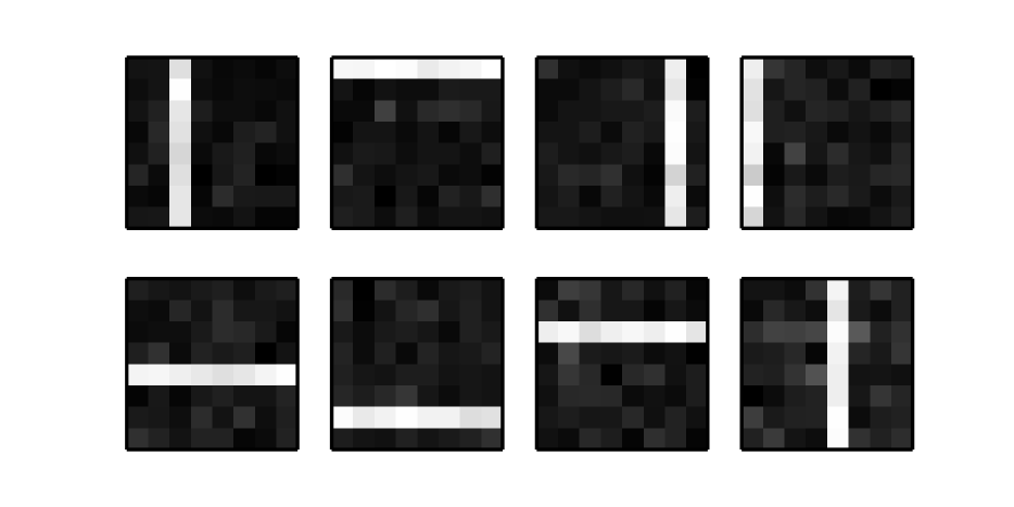
First, we perform clustering on a synthetic data set of $8\times 8$ images to show that ADF-NRM can recover the correct component distributions. Each image is represented by a vector of positive integer pixel intensities, which we interpret as a document over a vocabulary with $64$ terms. The clusters correspond to horizontal and vertical bars with an additive baseline to ensure cluster overlap. Each of 200 images is generated by first choosing a cluster, $z_{d}$, and then sampling pixel intensities $x_{d}\sim\mathrm{Mult}(50,\theta^{z_{d}})$. Fig. 1 depicts the resulting ADF-NRM posterior mean mixture components under the learned variational distribution, $\mathbb{E}_{\hat{q}_{N}}[\theta_{k}]$, based on an IG prior ($\sigma=0.5$), both with and without merge moves. We see that in both cases the algorithm learns the correct clusters, but merge moves remove redundant and extraneous clusters.

4.2 Synthetic Power-Law Clusters

To explore the benefit of the additional flexibility of IGs over DPs, we generated 10,000 synthetic documents, $x_{d}$, from a Pitman-Yor$(.75,1)$ mixture of multinomials. The Pitman-Yor prior is another commonly used BNP prior famous for its ability to model clusters whose sizes follow certain power-law distributions [18].

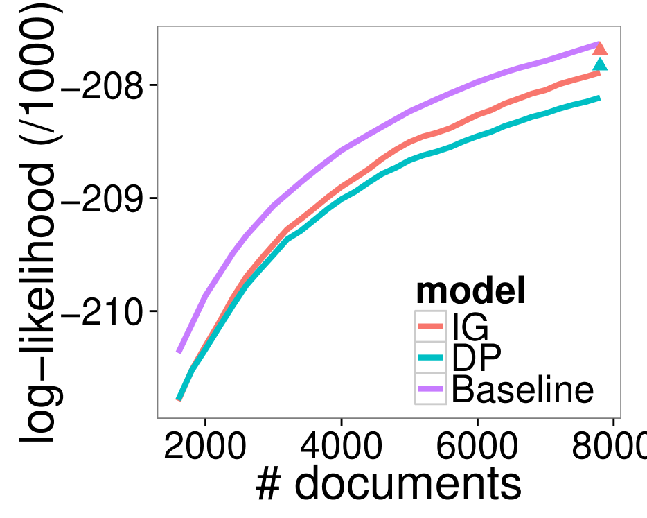
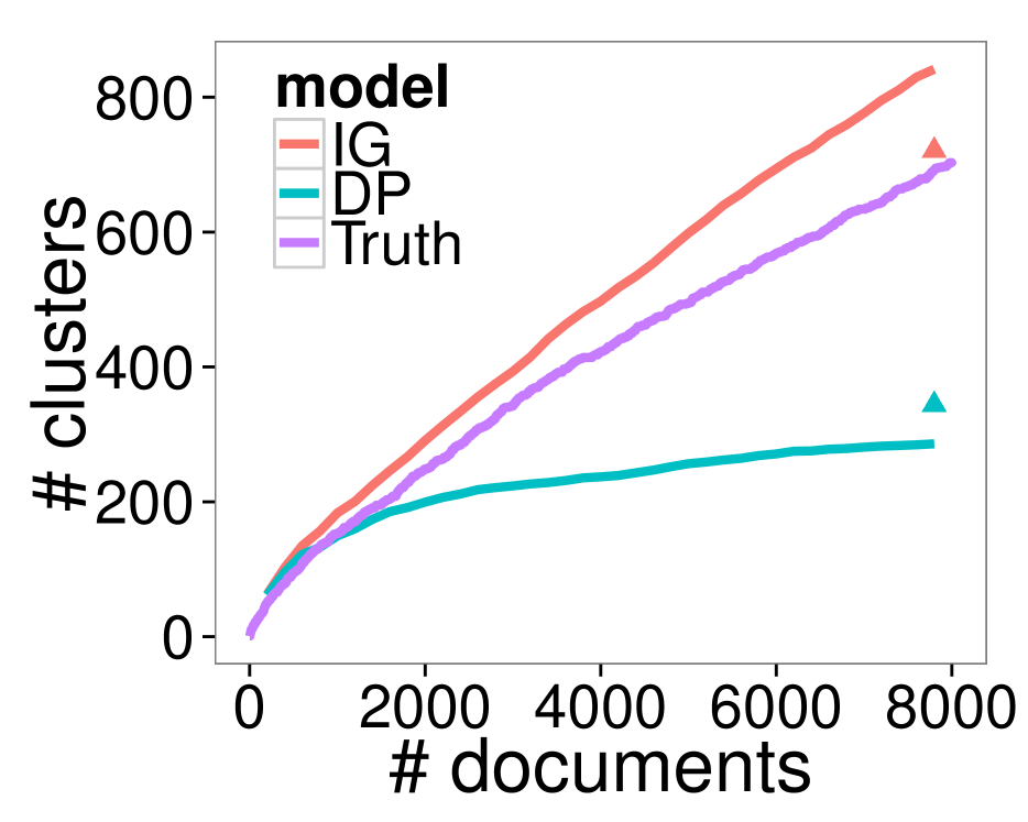
We assess the ADF-NRM predictive log-likelihood and inferred number of clusters versus number of observed documents. For each model, we selected hyperparameters based on a randomly selected set of $1,000$ documents. We then continue our algorithm on $7,000$ training documents and use the remaining $2,000$ for evaluation. Mean predictive log-likelihoods, number of clusters, and error estimates were obtained by permuting the order of the training documents 5 times. We compare our ADF-NRM performance to that of a baseline model where the cluster parameters are inferred based on ground-truth-labeled training data. Lastly, after the completion of ADF, we performed 49 additional passes through the data using EP-NRM to obtain refined predictions and number of clusters.

We see in Fig. 2 that both the IG and DP models perform similarly for small $n$, but as the amount of data increases, the IG provides an increasingly better fit in terms of both predictive log-likelihood and number of clusters. This substantiates the importance of our streaming algorithm being able to handle a broad class of NRMs. Furthermore, after a single data pass, ADF-NRM comes close to reaching the baseline model even with the IG/Pitman-Yor model mismatch. It is also evident in Fig. 2 that additional EP iterations both improve predictions and the match between inferred and true number of clusters for both prior specifications.

Figure 2: Mean predictive log-likelihood (left) and number of clusters (right) for the DP (cyan) and IG (red) priors on the synthetic power-law data set using ADF-NRM. Triangles indicate final values for EP-NRM after 50 epochs. The ground-truth model is shown in purple. Error bars are omitted due to their small size relative to the plot scale.

4.3 KOS Blog Corpus

Table 1: Mean predictive performance and number of clusters ($\pm$ 1 std. err.) for ADF-NRM, EP-NRM, and a collapsed Gibbs sampler on the KOS corpus.

Method	Pred. log-lik	#Clusters	Epochs
ADF-DP	-346023 $\pm$ 165	80 $\pm$ .17	1
ADF-IG	-345588 $\pm$ 159	92 $\pm$ .18	1
EP-DP	-342535 $\pm$ 181	104 $\pm$ 2.4	50
EP-IG	-342195 $\pm$ 161	114 $\pm$ 1.5	50
Gibbs-DP	-342164 $\pm$ 11	119 $\pm$ 0.3	215
Gibbs-IG	-341468 $\pm$ 338	128 $\pm$ 1.3	215

We also applied ADF-NRM to cluster the KOS corpus of 3,430 blog posts [19]. The fact that the corpus is small enough to use non-streaming (batch) inference algorithms allows us to compare ADF-NRM, EP-NRM, and the collapsed Gibbs sampler for NGGP mixture models presented in [5]. Importantly, we only compare to Gibbs, which is not suited to the streaming setting, in an attempt to form a gold standard. (Recall that Gibbs targets the exact posterior in contrast to our variational-based approach, and we do not expect mixing to be an issue in this modest-sized data set.)

We evaluated performance as in Sec. 4.2. Here, we held out $20\%$ of the entire corpus as a test set and trained (given the hyperparameters determined via grid search) on the remaining $80\%$ of documents. The ADF-NRM predictive log-likelihoods for the IG and DP were computed after a single pass through the data set while those for EP-NRM were computed by cycling through the data set 50 times. Error estimates were obtained by permuting the order of the documents 20 times. Predictions for the collapsed Gibbs sampler were computed by running 5 chains for 215 passes through the data and averaging the predictive log-likelihood for the last 50 samples across chains.

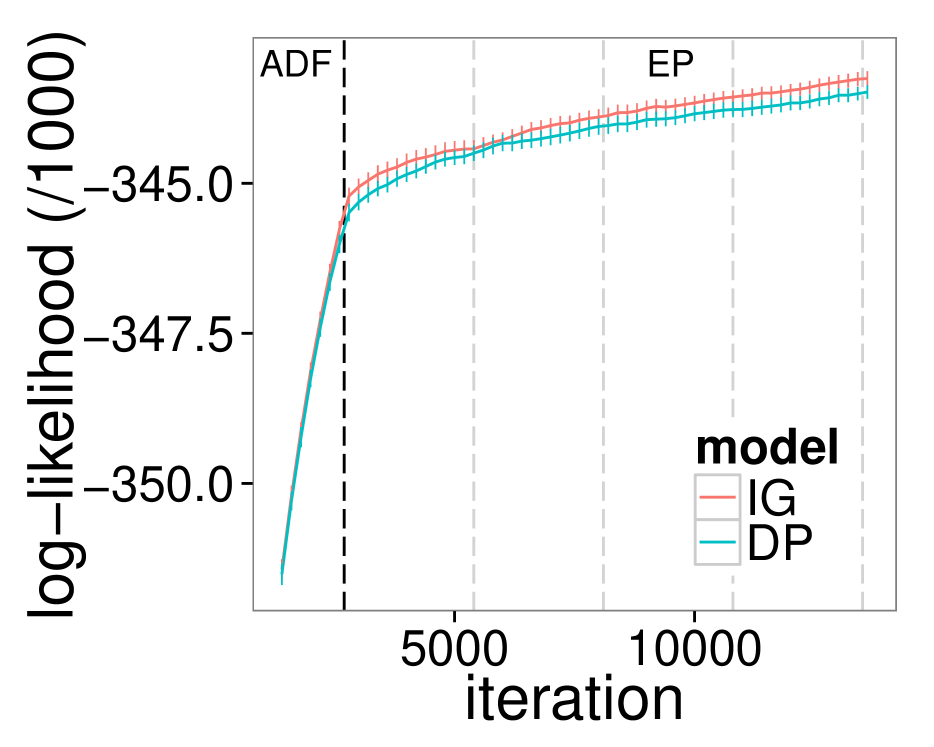
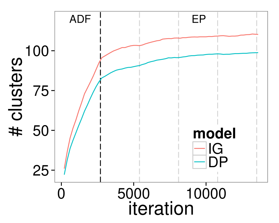
The comparisons between all methods are depicted in Table 1. For all algorithms (ADF, EP, and Gibbs) the added flexibility of the IG provides a better fit in terms of predictive log-likelihood. The extra $\approx 10$ clusters associated with the IG for all algorithms correspond to small clusters which seem to capture finer-scale latent structure important for prediction. Although performance increases moving from the one-pass ADF-NRM to multi-pass EP-NRM, Fig. 3 shows that the most gains occur in the first epoch. In fact, after one epoch ADF performs significantly better than a single epoch of Gibbs; it takes about three Gibbs epochs to reach comparative performance (see Supplement). Finally, while the IG Gibbs sampler leads to the best performance, EP-NRM with the IG prior is competitive and reaches similar performance to the DP using Gibbs.

In summary, ADF-NRM provides competitive performance with only a single pass through the data; refined approximations nearly matching the computationally intensive samplers can be computed via EP-NRM if it is feasible to save and cycle through the data.

Figure 3: Predictive log-likelihood (left) and mean number of clusters (right) using EP-NRM on KOS corpus. Vertical lines indicate epochs and error bars $\pm$ 1 st. dev..

4.4 New York Times Corpus

We performed streaming inference on a corpus of 300,000 New York Times articles [19]. We first identified a vocabulary of $7,841$ unique words by removing words occurring in fewer than 20 and more than $90\%$ of documents, as well as terms resulting from obvious errors in data acquisition. Then, we removed documents containing fewer than 20 words in our vocabulary, resulting in a corpus of 266,000 documents. The corpus is too large for batch algorithms, so we focus on ADF-NRM comparing the DP and IG priors.

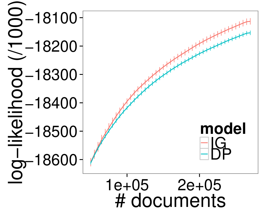
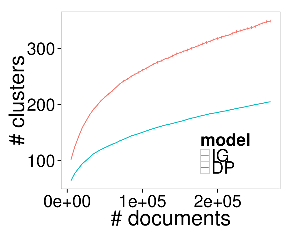
We determined hyperparameters as before and held out $5,000$ documents as a test set, evaluating the predictive log-likelihood and number of clusters after every $5,000$ training documents were processed. See Fig. 4. As before, the IG obtains superior predictive log-likelihood and introduces many additional small clusters compared to the DP, suggesting that the IG may be capturing nuanced latent structure in the corpus that the DP cannot (see the Supplement for details). Reassuringly, the recovered clusters with highest weights correspond to interpretable topics (Fig. 5). Again, we see the benefits of considering NRMs beyond the DP, which has been the most used BNP prior due to the computational tools developed for it.

Figure 4: Comparison of (left) predictive log-likelihood and (right) number of clusters using ADF-NRM on the New York Times corpus for the IG and DP priors.

Figure 5: Most probable words and their respective contributions (in %) for the $4$ most prevalent topics.

5 Discussion

We introduced the ADF-NRM algorithm, a variational approach to streaming approximate posterior inference in NRM-based mixture models. Our algorithm leverages the efficient sequential updates of ADF while importantly maintaining the infinite-dimensional nature of the BNP model. The key to tractability is focusing on approximating a partial-urn characterization of the NRM predictive distribution of cluster assignments. We also showed how to adapt the single-pass ADF-NRM algorithm to a multiple-pass EP-NRM variant for batch inference. Our empirical results demonstrated the effectiveness of our algorithms, and the importance of considering NRMs beyond the DP.

A potential drawback of the EP-NRM scheme is that each observation needs to store its variational distribution over cluster assignments. An interesting question is if the local distributions can be grouped and memoized [20] to save computation and perform data-driven split-merge moves. This combined with parallel EP [14, 21] would scale EP-NRM to massive data sets.

Instead of using predictive distributions and exploiting the NRM partial-urn scheme, a natural question is if similar algorithms can be developed that do not integrate out the underlying measure. Such algorithms would be applicable to hierarchical BNP models such as topic models and hidden Markov models [22].

Acknowledgements: This work was supported in part by DARPA Grant FA9550-12-1-0406 negotiated by AFOSR, ONR Grant N00014-10-1-0746, and the TerraSwarm Research Center sponsored by MARCO and DARPA. AT was partially funded by an IGERT fellowship.

 

Supplemental Information: Streaming Variational Inference for Bayesian Nonparametric Mixture Models

 

1 Derivation of Global Update

This section motivates the use of the mean field update for the global variables, given in Eq. (18) of the main text, as an approximation to the optimal update for ADF after adding in the likelihood factor. The presentation adapts that of [15] for ADF-NRM.

Let $\hat{p}(\theta,z_{1:n}|x_{1:n})\propto p(x_{n}|\theta,z_{n})q^{\text{pr}}(z_{1:n},\theta)$ denote the approximate posterior under the past variational updates after adding in the $n$th observation/likelihood factor. The optimal $q(\theta_{k})$ under ADF is given by the marginal distribution of $\hat{p}$:

$$\hat{q}_{n}(\theta_{k})\propto \int\sum_{z_{1:n}}\hat{p}(\theta_{k}|\theta_{\setminus k},z_{1:n},x_{1:n})\times$$ (1)

$$\hat{p}(\theta_{\setminus k}|z_{1:n},x_{1:n})\hat{p}(z_{1:n}|x_{1:n})d\theta_{\setminus k}.$$

Both the sums and integrals are intractable so we use the approximations: $\hat{p}(\theta_{\setminus k}|z_{1:n},x_{1:n})\approx\hat{q}_{n}(\theta_{\setminus k})$ and $\hat{p}(z_{1:n}|x_{1:n})\approx\hat{q}_{n}(z_{1:n})=\prod_{i=1}^{n}\hat{q}_{n}(z_{i})$ which yields:

$$\hat{q}_{n}(\theta_{k}) \stackrel{{\scriptstyle\approx}}{{\propto}}\int\sum_{z_{1:n}}\hat{p}(\theta_{k}|\theta_{\setminus k},z_{1:n},x_{1:n})\hat{q}_{n}(\theta_{\setminus k})\hat{q}_{n}(z_{1:n})d\theta_{\setminus k}$$

$$=E_{\hat{q}_{n}(z_{1:n}),\hat{q}_{n}(\theta_{\setminus k})}[\hat{p}(\theta_{k}|\theta_{\setminus k},z_{1:n},x_{1:n})]$$

$$=\exp\{\log E_{\hat{q}_{n}(z_{1:n}),\hat{q}_{n}(\theta_{\setminus k})}[\hat{p}(\theta_{k}|\theta_{\setminus k},z_{1:n},x_{1:n})]\}$$

$$\leq\exp\{E_{\hat{q}_{n}(z_{1:n}),\hat{q}_{n}(\theta_{\setminus k})}[\log\hat{p}(\theta_{k}|\theta_{\setminus k},z_{1:n},x_{1:n})]\}$$

$$\propto\exp\{E_{\hat{q}_{n}(z_{1:n}),\hat{q}_{n}(\theta_{\setminus k})}[\log\hat{p}(\theta,z_{1:n}|x_{1:n})]\}$$ (2)

where the inequality follows by Jensen’s inequality [15]. The approximation is tight when $\hat{q}(z_{1:n})$ and $\hat{q}(\theta_{\setminus k})$ approach Dirac measures. Eq. (2) is that of the standard mean field update for $\hat{q}(\theta_{k})$ [23]. Since the $q(\theta_{k})$ distributions are unknown for all $k$, we could perform coordinate ascent and cycle through these updates for each of the $\theta_{k}$ given the other $\theta_{\setminus k}$ and $\hat{q}(z_{1:n})$. Conveniently, since the $\hat{q}(z_{1:n})$ is already optimized by its tractable marginal, the $\theta_{k}$s are conditionally independent given the assignments in the mixture model, and $q^{\text{pr}}(z_{1:n},\theta)=q^{\text{pr}}(z_{n})\prod_{i=1}^{n-1}\hat{q}_{i}(z_{i})\prod_{k=1}^{\infty}\hat{q}_{n-1}(\theta_{k})$, we can perform a single mean field update for each $\theta_{k}$ given by,

$$\hat{q}_{n}(\theta_{k})\propto p(x_{n}|z_{nk},\theta)^{\hat{q}_{n}(z_{nk})}\hat{q}_{n-1}(\theta_{k}).$$ (3)

2 Derivation of approximate NRM predictive rule

In this section we provide the derivation of $q^{\mathrm{pr}}(z_{n})$ for NRMs given in Eq. (25) of the main text. We start by presenting the derivation for general NRMs and then demonstrate how to apply ideas to NGGPs. The presentation in this section is adapted from [5, 11].

2.1 General NRMs

We assume the mixture model specification in Eq. (3) from the main text. In particular we note that the unnormalized mixture weights $\pi=(\pi_{1},\pi_{2},\ldots)$ are drawn from a completely random measure with Lévy measure $\lambda(d\pi)$. We also introduce the exponentially tilted Lévy measure as $e^{-U\pi}\lambda(d\pi)$ which will appear below.

First, we expand the sum in the approximate predictive distribution, $q^{\mathrm{pr}}(z_{n})$, to include the unnormalized masses, $\pi$, and the auxiliary variable $U_{n-1}$:

$$q^{\mathrm{pr}}(z_{n}) =\sum_{z_{1:n-1}}p(z_{n}|z_{1:n-1})\prod_{i=1}^{n-1}\hat{q}_{n-1}(z_{i})$$ (4)

$$=\sum_{z_{1:n-1}}\iint p(z_{n}|\pi)p(\pi|U_{n-1},z_{1:n-1})$$ (5)

$$\times p(U_{n-1}|z_{1:n-1})dU_{n-1}d\pi\prod_{i=1}^{n-1}\hat{q}_{n-1}(z_{i})$$

where the conditional distribution of the auxiliary variables $U_{n-1}$ given the past assignments is given by:

$$p(U_{n-1}|z_{1:n-1})=U_{n-1}^{n-1}e^{-\phi(U_{n-1})}\prod_{k=1}^{K_{n-1}}\kappa_{n_{k}}(U_{n-1})$$ (6)

where $\phi(U)$ is the Laplace exponent of the underlying CRM, $\phi(U)=\int(1-e^{-Us})\lambda(ds)$, and $\kappa_{m}(U)$ denotes the $m$th moment of the exponentially tilted Lévy measure, $\kappa_{m}=\int s^{m}e^{-Us}\lambda(ds)$.

Let $K_{n-1}$ denote the number of components considered for the observations $z_{1:n-1}$. The conditional distribution of the random measure, $\pi=(\pi^{*},\pi_{1},\ldots,\pi_{K_{n-1}})$, given $U_{n-1}$ and the assignments, $z_{1:n-1}$, is:

$$p(\pi|U_{n-1},z_{1:n-1}) =p(\pi^{*}|U_{n-1})\prod_{k=1}^{K_{n-1}}p(\pi_{k}|z_{1:n-1},U_{n-1}).$$ (7)

where $\pi_{1:K_{n-1}}$ are the masses of all the instantiated components and $\pi^{*}$ denotes the mass assigned to the uninstantiated components. The distribution of $\pi_{k}$ is given by

$$p(\pi_{k}|z_{1:n-1},U_{n-1})\propto\pi_{k}^{n_{k}}e^{-U_{n-1}\pi_{k}}\lambda(d\pi_{k}),$$ (8)

where $n_{k}$ is the number of observations assigned to component $k$ in $z_{1:n-1}$ and $\pi^{*}$ follows a Poisson process (PP) with exponentially tilted Lévy measure, $\pi^{*}\sim\mathrm{PP}(e^{-U_{n-1}\pi^{*}}\lambda(d\pi^{*}))$, where again $\lambda(ds)$ is the Lévy measure of the unnormalized masses. Since the integral in Eq (2.1) is intractable, we introduce a variational approximation for $\pi$ and $U_{n-1}$. In particular, we use a partially factorized approximation

$$p(\pi|U_{n-1},z_{1:n-1})p(U_{n-1}|z_{1:n-1})\hat{q}(z_{1:n-1})\approx$$ (9)

$$q(\pi|U_{n-1})q(U_{n-1})\hat{q}(z_{1:n-1}),$$

where $\hat{q}(z_{1:n-1})=\prod_{i=1}^{n-1}\hat{q}_{n-1}(z_{i})$ is fixed and given from previous iterations. We perform a mean field step to minimize the KL divergence between the left and right hand sides of Eq (9). Specifically, we compute the optimal $q(U_{n-1})$ and then given that we compute the optimal $q(\pi|U_{n-1})$. Because of the factorization given in the left hand of Eq. (9) this procedure gives the optimal distributions. According to standard mean field updates the optimal distribution for $q(U_{n-1})$ is given by:

$$\log q(U_{n-1})=E_{\hat{q}(z_{1:n-1})}\log p(U_{n-1}|z_{1:n-1})+C$$ (10)

where $p(U_{n-1}|z_{1:n-1})$ is given in Eq. (6). The tractability of this variational approximation for $U_{n-1}$ will depend on the NRM under consideration. For the NGGP it is conveniently given in closed form, as detailed below in Section 2.2. However, efficient numerical algorithms can be used to compute the necessary integrals for general NRMs.

Given the optimal $q(U_{n-1})$, the optimal variational approximations to the masses, $q(\pi|U_{n-1})=q(\pi^{*}|U_{n-1})\prod_{i=1}^{K_{n-1}}q(\pi_{j}|U_{n-1})$, are given by

$$q(\pi_{k}|U_{n-1})\propto\pi_{k}^{\mathbb{E}_{\hat{q}}[n_{k}]}e^{-U\pi_{k}}\lambda(d\pi_{k})\mbox{ for $k=1\ldots K_{n-1}$},$$ (11)

where $\mathbb{E}_{\hat{q}}[n_{k}]$ is the expected number of assignments to component $k$ and is given by:

$$\mathbb{E}_{\hat{q}}[n_{k}]=\sum_{i=1}^{n-1}\hat{q}(z_{ik}).$$ (12)

Under $q(\pi^{*}|U_{n-1})$, $\pi^{*}$ is still drawn from $\mathrm{PP}(e^{-U_{n-1}w}\lambda(dw))$. Using these approximations Eq. (2.1) becomes

$$q^{\mathrm{pr}}(z_{n}) =\sum_{z_{1:n-1}}\iint p(z_{n}|\pi)p(\pi|U,z_{1:n-1})$$ (13)

$$\times p(U_{n-1}|z_{1:n-1})dU_{n-1}d\pi\prod_{i=1}^{n-1}\hat{q}_{n-1}(z_{i})$$

$$\approx\iint p(z_{n}|\pi)q(\pi|U_{n-1})q(U_{n-1})d\pi dU_{n-1}$$ (14)

$$=\int q(z_{n}|U_{n-1})q(U_{n-1})dU_{n-1}$$ (15)

where

$$q(z_{nk}|U_{n-1})\propto\begin{cases}\max\left(\frac{\kappa_{E_{\hat{q}}[n_{k}]+1}(U_{n-1})}{\kappa_{\mathbb{E}_{\hat{q}}[n_{k}]}(U_{n-1})},0\right),\,\text{$k\leq K_{n-1}$}\\ \kappa_{1}(U_{n-1}),\,\,\,\,\,\,\,\,\,\,\,\,\,\,\,\,\,\,\,\,\,\,\,\,\,\,\,\text{$k=K_{n-1}+1$}.\end{cases}$$ (16)

Eq. (15) arises from (14) by an application of Prop. 2.1 in [5]. In Eq. (16), the maximum with zero is necessary since if the expected number of clusters assigned to a cluster $k$, $\mathbb{E}_{\hat{q}}[n_{k}]$, is small then the variational distribution for $\pi_{k}$ given in Eq. (11) might be degenerate at zero and so there will be zero probability of a new observation being assigned to that cluster. More details for the NGGP case are given in Section 2.2.

2.2 Predictive Rule for the NGGP

For NGGPs, the general equations for NRMs described above reduce to simple, analytically tractable forms. In particular, the variational approximation $q(U_{n-1})$ is given by

$$q(U_{n-1})\propto\frac{U_{n-1}^{n-1}}{(U_{n-1}+\tau)^{n-1-a\mathbb{E}_{\hat{q}(z_{1:n-1})}[K_{n-1}^{\prime}]}}e^{-\frac{a}{\sigma}(U_{n-1}+\tau)^{\sigma}}$$ (17)

where $\mathbb{E}_{\hat{q}(z_{1:n-1})}[K^{\prime}_{n-1}]$ is the expected number of clusters instantiated thus far. This expectation is given by:

$$\mathbb{E}_{\hat{q}(z_{1:n-1})}[K_{n-1}^{\prime}] =K_{n-1}-\sum_{j=1}^{K_{n-1}}\left(\prod_{i=1}^{n-1}(1-\hat{q}(z_{ij}))\right)$$ (18)

$$\stackrel{{\scriptstyle n\to\infty}}{{\to}}K_{n-1}.$$ (19)

Note that Eq. (18) does not require all past soft assignments to be saved; instead, only $\prod_{i=1}^{n-1}(1-\hat{q}(z_{ij}))$ must be stored for each component and updated after each observation. In practice we find that using $\mathbb{E}_{\hat{q}(z_{1:n-1})}[K_{n-1}^{\prime}]\approx K_{n-1}$ leads to comparable performance to evaluating the complete expectation. This occurs because, given our thresholding scheme for mixture components, each component has a few $\hat{q}(z_{ik})$ that are close to one, making the product close to zero.

Additionally, in the case of the NGGP the $\kappa_{m}(U)$ functions needed in Eq. (15) are given by

$$\kappa_{m}(U)=\frac{a}{(U+\tau)^{m-\sigma}}\frac{\Gamma(m-\sigma)}{\Gamma(1-\sigma)},$$ (20)

which when plugged into Eq. (16) yields

$$q(z_{nk}|U_{n-1})\propto\begin{cases}\max\left(\sum_{i=1}^{n-1}\hat{q}(z_{ik})-\sigma,0\right),\,\text{$k\leq K_{n-1}$}\\ a(U_{n-1}+\tau)^{\sigma},\,\,\,\,\,\,\,\,\,\,\,\,\,\,\,\,\,\,\,\,\,\,\text{$k=K_{n-1}+1$}.\end{cases}$$ (21)

When we approximate the integral in Eq. (15) with a delta function about the maximum, $\hat{U}_{n-1}=\arg\max q(U_{n-1})$ we see that $q^{\mathrm{pr}}(z_{nk})\approx q(z_{nk}|\hat{U}_{n-1})$, which is exactly Eq. (25) of the main text. Alternatively, one could compute the integral in Eq. (15) numerically by first performing a change of variables, $V_{n-1}=\log U_{n-1}$, to obtain a log-convex density over $V_{n-1}$ and then use adaptive rejection sampling to sample from $V_{n-1}$, as proposed in [5]. The efficiency of this method depends on the sampling process and we leave such investigations to future work. Intuitively, $q(z_{nk}|U_{n-1})=0$ for some $k$ when $\sum_{i=1}^{n-1}\hat{q}_{i}(z_{ik})<\sigma$ since $q(\pi_{k}|U_{n-1})$ will be degenerate in Eq. (11). This means that $\sigma$ acts as a natural threshold for the instantiated clusters as clusters with mass (under the variational distribution) smaller than $\sigma$ will have zero probability of having observations assigned to it.

3 EP-NRM derivation

In this section we modify the EP derivation in [6] for our EP-NRM algorithm for batch inference. The resulting algorithm is conceptually similar to ADF-NRM, except now we also save a local contribution to the variational approximation for each data point. The algorithm cycles through the observations repeatedly, refining the variational approximations for $z_{1:N}$ and $\theta$. Due to the fact that local contributions must be saved, the algorithm is applicable to moderately sized data sets. The full EP-NRM algorithm is shown in Alg. 2.

Assume we have an approximation to the batch posterior

$$p(\theta,z_{1:N}|x_{1:N}) \approx\hat{q}(\theta,z_{1:N})$$ (22)

$$=\prod_{k=1}^{\infty}\hat{q}(\theta_{k})\prod_{i=1}^{N}\hat{q}(z_{i})$$ (23)

$$\propto\prod_{i=1}^{N}\bar{q}_{i}(\theta,z_{1:n}),$$ (24)

where $\bar{q}_{i}(\theta,z_{1:n})$ are the local contributions as described in the main text. Furthermore, assume that

$$\bar{q}_{i}(\theta,z_{1:n}) =\bar{q}_{i}(z_{i})\prod_{k=1}^{\infty}\bar{q}_{i}(\theta_{k})$$ (25)

and that $\bar{q}_{i}(z_{i})=\hat{q}(z_{i})$. This holds initially since since $\bar{q}_{i}(\theta,z_{1:n})$ is initialized during ADF to $\bar{q}_{i}(\theta,z_{1:n})\propto\frac{\hat{q}_{i}(\theta,z_{1:i})}{\hat{q}_{i-1}(\theta,z_{1:i-1})}$. Since $\bar{q}_{i}(\theta,z_{1:N})$ only depends on $z_{i}$ we henceforth refer to this quantity as $\bar{q}_{i}(\theta,z_{i})$. Under these assumptions we can rewrite the approximation to the full posterior excluding data point $i$ as

$$\hat{q}_{\setminus i}(\theta,z_{\setminus i}) \propto\frac{\hat{q}(\theta,z_{1:N})}{\bar{q}_{i}(\theta,z_{i})}$$ (26)

$$=\frac{\prod_{k=1}^{\infty}\hat{q}(\theta_{k})\prod_{j=1}^{n}\hat{q}(z_{j})}{\hat{q}(z_{i})\prod_{k=1}^{\infty}\bar{q}_{i}(\theta_{k})}$$ (27)

$$=\prod_{k=1}^{\infty}\frac{\hat{q}(\theta_{k})}{\bar{q}_{i}(\theta_{k})}\prod_{j\neq i}\hat{q}(z_{j}).$$ (28)

$$=\prod_{k=1}^{\infty}\hat{q}_{\setminus i}(\theta_{k})\prod_{j\neq i}\hat{q}(z_{j}).$$ (29)

The EP-NRM algorithm consists of the following two steps. First, update the global variational approximations, $\hat{q}(\theta_{k})$ and $\hat{q}(z_{i})$. Second, use these to refine $\bar{q}_{i}(\theta_{k})$ and $\bar{q}_{i}(z_{i})$ (see Alg. 2). The global variational approximations are themselves updated using the two step procedure specified in Section 3 of the main text. Specifically, we first form $\hat{p}(z_{1:N},\theta)|x_{\setminus i})\stackrel{{\scriptstyle\triangle}}{{\propto}}p(z_{i}|z_{\setminus i})\hat{q}_{\setminus i}(\theta,z_{\setminus i})$, and solve

$$q^{\text{pr}}(z_{1:n},\theta)=\operatorname*{arg\,min}_{q\in\mathcal{Q}}\mathrm{KL}\Big{(}\hat{p}(z_{1:N},\theta|x_{\setminus i})||q(z_{1:n},\theta)\Big{)}.$$ (30)

We then form $\hat{p}(z_{1:N},\theta)|x_{1:N})\stackrel{{\scriptstyle\triangle}}{{\propto}}p(x_{i}|z_{i},\theta)q^{\text{pr}}(z_{1:n},\theta)$ and solve

$$\hat{q}(z_{1:N},\theta)=\operatorname*{arg\,min}_{q\in\mathcal{Q}}\mathrm{KL}\Big{(}\hat{p}(z_{1:N},\theta|x_{1:N})||q(z_{1:n},\theta)\Big{)}.$$ (31)

As in ADF-NRM $\hat{q}(z_{j})$ for $j\neq i$ terms are unchanged; the optimal update for $\hat{q}(z_{i})$ is given by:

$$\hat{q}(z_{ik})\propto q^{\mathrm{pr}}(z_{ik})\int p(x_{i}|z_{ik},\theta_{k})\hat{q}(\theta_{k})d\theta_{k}\;\;\;k=1,\ldots,K+1,$$ (32)

where $K$ is the number of instantiated clusters and $\hat{q}(\theta_{K+1})=p(\theta_{K+1})$. Similar to ADF, the predictive distribution for the NGGP in Eq.(32) is given by:

$$q^{\mathrm{pr}}_{\setminus i}(z_{ik}){\propto}\begin{cases}\displaystyle\max\left(\sum_{i\neq j}\hat{q}(z_{jk})-\sigma,0\right),&k\leq K\\ a(\hat{U}_{\setminus i}+\tau)^{\sigma},&k=K+1\end{cases}$$ (33)

where $q(U_{\setminus i})$ is given by:

$$q(U_{\setminus i})\propto\frac{U_{\setminus i}^{N-1}}{(U_{\setminus i}+\tau)^{N-1-a\mathbb{E}_{\hat{q}(z_{\setminus i})}[K^{\prime}]}}e^{-\frac{a}{\sigma}(U_{\setminus i}+\tau)^{\sigma}}.$$ (34)

where $K^{\prime}$ is the number of unique assignments in $z_{\setminus i}$ and $\hat{U}_{\setminus i}=\arg\max q(U_{\setminus i})$.

Following the ADF discussion in the main text, the optimal variational distributions for the $\theta_{k}$s are given by:

$$\hat{q}(\theta_{k})\propto p(x_{i}|z_{ik},\theta_{k})^{\hat{q}(z_{ik})}\hat{q}_{\setminus i}(\theta_{k}).$$ (35)

Given updated approximations $\hat{q}(\theta_{k})$ and $\hat{q}(z_{i})$, the local contribution for observation $i$ is refined as:

$$\bar{q}_{i}(\theta,z_{i}) =\frac{\hat{q}(\theta,z_{1:N})}{\hat{q}_{\setminus i}(\theta,z_{\setminus i})}$$ (36)

$$=\hat{q}(z_{ik})\prod_{k=1}^{\infty}p(x_{i}|z_{ik},\theta_{k})^{\hat{q}(z_{ik})}$$ (37)

$$=\bar{q}_{i}(z_{i})\prod_{k=1}^{\infty}\bar{q}_{i}(\theta_{k})$$ (38)

which takes the form we assumed in Eq. (25).

When $\hat{q}(\theta_{k})$ is in the exponential family with sufficient statistics $\hat{\nu}^{k}$, then Eqs. (28) and (36) are given adding and subtracting the corresponding sufficient statistics [6].

Algorithm 2 EP-NRM algorithm

  $\hat{q}(\theta_{1:K}),S_{1:K},\bar{q}(z_{1:N}),\bar{q}_{1:N}(\theta_{1:K})\leftarrow$ ADF-NRM$(x_{1:N})$ // Initialize via ADF with data contributions.

  while $\hat{q}(\theta_{1:K})$ not converged do

     for $i=1$ to $N$ do

        $\hat{U}_{\setminus i}=\operatorname*{arg\,max}q(U_{\setminus i})$

        for $k=1$ to K do

           $S_{k}=S_{k}-\bar{q}_{i}(z_{ik})$

           $q^{\mathrm{pr}}(z_{ik})\propto\max(S_{k}-\sigma,0)$

           $\hat{q}_{\setminus i}(\theta_{k})\propto\frac{\hat{q}(\theta_{k})}{\bar{q}_{i}(\theta_{k})}$

           $\hat{q}(z_{ik})\propto q^{\mathrm{pr}}(z_{ik})\int p(x_{i}|z_{ik},\theta_{k})\hat{q}_{\setminus i}(\theta_{k})d\theta_{k}$.

        end for

        $q^{\mathrm{pr}}(z_{i,K+1})\propto a(\hat{U}_{\setminus i}+\tau)^{\sigma}$

        $\hat{q}(z_{i,K+1})\propto q^{\mathrm{pr}}(z_{i,K+1})\int p(x_{i}|z_{i,K+1},\theta)p(\theta_{K+1})d\theta_{K+1}$

        normalize $\hat{q}(z_{i(1:K+1)})$

        if $\hat{q}(z_{i,K+1})>\epsilon$ then

           $K=K+1$, $S_{K}=0$, $\hat{q}(\theta_{K})=p(\theta_{K})$

        else

           normalize $\hat{q}(z_{i(1:K)})$

        end if

        for $k=1$ to $K$ do

           $\hat{q}(\theta_{k})\propto p(x_{i}|z_{ik},\theta_{k})^{\hat{q}(z_{ik})}\hat{q}_{\setminus i}(\theta_{k})$

           $S_{k}=S_{k}+\hat{q}(z_{ik})$

           $\bar{q}_{i}(z_{ik})=\hat{q}(z_{ik})$

           $\bar{q}_{i}(\theta_{k})\propto p(x_{i}|z_{ik},\theta_{k})^{\hat{q}(z_{ik})}$

        end for

        Remove all clusters for which $S_{k}<\epsilon$

     end for

  end while

4 Experiments

In this section we provide details on how we select hyperparameter values of the IG and DP for the experiments in the main text. We also present additional experimental results regarding the convergence of EP-NRM and comparisons with the Gibbs sampler.

4.1 Selecting Hyperparameters: $a$, $\tau$, and $\alpha$

In order to compare the modeling performance of the IG and DP on the document corpora considered in the main text, we must first select the values of the hyperparameters, $a$ and $\tau$ (since $\sigma$ is known in both cases). It is well known that the hyperparameters of both the IG ($a$ and $\tau$) and the DP ($a$) strongly affect the posterior distribution over the number of inferred clusters. For all experiments where the IG and DP are compared we adapt a method to determine the hyperparameters for GGP mixture models originally developed for batch inference [4] to the streaming setting of interest. Specifically, for a given corpus, we consider a small subset of the entire corpus (5% for the NYT corpus and 10% for both the KOS and synthetic data) which we then split into a training and testing sets used to determine the hyperparameters. We run ADF-NRM on the training portion of the subset of documents (95% of the subset for NYT and 80% for both KOS and synthetic data) for a grid of parameters $a\in[1,10,100,1000]$ and $\tau\in[.1,1,10,100,1000]$. For the DP we only consider $a$ and for the IG we consider both $a$ and $\tau$. For each parameter value we compute the heldout log-likelihood of the test portion of the subset and choose the values of $a$ and $\tau$ with the largest heldout log-likelihood to use when running ADF-NRM and EP-NRM on the remainder of the corpora. This setup mimics a streaming scenario in that an initial subset of the data is collected for preliminary analysis and then the algorithm is let loose on the entire data set as it arrives.

For the Pitman-Yor data set, the grid search resulted in $a=100$ for the DP and $a=1,\tau=1000$ for the IG. The resulting parameter values for the KOS corpus were $a=100$ for the DP and $a=10,\tau=100$ for the IG. Last, on the NYT corpus we obtained the parameter values $a=1000$ for the DP and $a=100,\tau=100$ for the IG.

In the synthetic bars experiments $\alpha$ was set to $0.5$, however correct recovery of the bars was robust to values within a reasonable range, $\alpha\in[0.1,0.9]$. For the Pitman-Yor synthetic data, the cluster centers were drawn from a Dirichlet with $\alpha=0.75$ to ensure overlap between clusters; $\alpha=0.75$ was used for inference as well. For the KOS corpus $\alpha=0.1$ was used because it was found to provide the best overall fit under repeated trials. Finally, for the NYT data set $\alpha=0.5$ was used, as is common for this corpus [15].

4.2 KOS Corpus

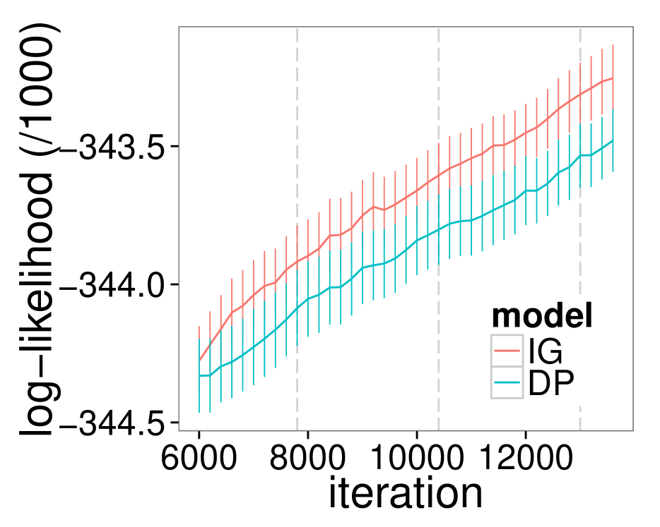
While the ADF-NRM algorithm makes a single pass through the corpus, a more accurate posterior approximation can be achieved by revisiting observations as in EP-NRM. Figure 1 shows the predictive performance for EP-NRM applied to the KOS corpus. We see a rapid increase in predictive performance in the first epoch which corresponds to ADF-NRM. Predictive performance continues to rise during subsequent epochs indicating an improved variational posterior.

Figure 1: (left) EP predictive performance on KOS corpus for both models continues to rise after the pass through the data (equivalent to ADF-NRM). The black vertical line indicates the completion of the first pass through the data. The other grey vertical lines indicate subsequent epochs. (right) Zoom in of the plot on the left.

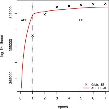
We compare the predictive performance of ADF-NRM, EP-NRM, and the Gibbs sampler for the IG model on the KOS corpus and present the results in Figure 2. In particular, we compare the predictive log-likelihood of held-out data versus the number of complete passes through the data (epochs). Both ADF-NRM and EP-NRM are initialized as in the main text and the Gibbs sampler is initialized so that all data points are assigned to a single component. We found this Gibbs initialization to outperform random cluster initialization. ADF-NRM performs significantly better than Gibbs after the first epoch and it takes three full epochs for Gibbs to outperform ADF-NRM and EP-NRM method. Both methods are implemented in Python and a per epoch timing comparison shows that ADF-NRM takes an average of 220 seconds per epoch while the Gibbs sampler takes an average of 160 seconds per epoch. The ADF-/EP-NRM methods take longer since the auxiliary variable $U$ must be updated after each data point has been processed, while in the collapsed sampler $U$ is only sampled once per epoch. Furthermore, in the Gibbs sampler, after a cluster assignment has been sampled only the sufficient statistics for the corresponding component must be updated, while in ADF-NRM, all component parameters are updated after every data point. Importantly, our goal is not to beat the Gibbs sampler, neither in performance nor compute time, but only to show that the streaming ADF-NRM reaches competitive performance to Gibbs after only a single pass through the data. Remember, Gibbs is inherently not suited to our streaming data of interest.

Figure 2: Comparison of the predictive performance of ADF-NRM, EP-NRM, and the Gibbs sampler for both the IG model. The predictive log-likelihood is plotted against the number of epochs through the KOS corpus.

4.3 New York Times

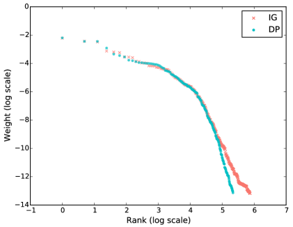
As seen in the main paper, the IG both introduces more clusters than the DP and attains superior predictive performance. To further explore the difference in the inferred clusters between the two models we plot the normalized variational cluster weights in decreasing order in Figure 3. In particular, let $S_{k}=\sum_{i=1}^{N}\hat{q}_{i}(z_{ik})$ be the total weight assigned to cluster $k$ after a full pass through the data and $\hat{p}_{k}=\frac{S_{k}}{\sum_{j=1}^{K_{N}}S_{j}}$ be the normalized weight. We can interpret $\hat{p}_{k}$ as the posterior probability of an observation being assigned to cluster $k$. We see in Figure 3 that the distribution of weights for the IG has a heavier tail than the DP. The plots are similar for the large and medium sized clusters but diverge for the small clusters, indicating that the IG emphasizes capturing structure at a finer scale.

Figure 3: Variational cluster weights in decreasing order. The IG exhibits a heavier tail than the DP.

References

- [1] M. D. Hoffman, D. M. Blei, C. Wang, and J. Paisley. Stochastic variational inference. J. Mach. Learn. Res., 14(1):1303–1347, May 2013.
- [2] T. Broderick, N. Boyd, A. Wibisono, A. C. Wilson, and M. I. Jordan. Streaming variational Bayes. In Advances in Neural Information Processing Systems, 2013.
- [3] D. Lin. Online learning of nonparametric mixture models via sequential variational approximation. In Advances in Neural Information Processing Systems. 2013.
- [4] E. Barrios, A. Lijoi, L. E. Nieto-Barajas, and I. Prünster. Modeling with normalized random measure mixture models. Statistical Science, 28(3):313–334, 2013.
- [5] S. Favaro and Y. W. Teh. MCMC for normalized random measure mixture models. Statistical Science, 28(3):335–359, August 2013.
- [6] T. Minka. Expectation propagation for approximate Bayesian inference. In Advances in Neural Information Processing Systems, 2001.
- [7] J. F. C. Kingman. Completely random measures. Pacific Journal of Mathematics, 21(1):59–78, 1967.
- [8] J. F. C. Kingman. Poisson Processes. Oxford University Press, 1993.
- [9] T. S. Ferguson. A Bayesian analysis of some nonparametric problems. Annals of Statistics, 1(2):209–230, 1973.
- [10] N. L. Hjort. Nonparametric Bayes estimators based on beta processes in models for life history data. Annals of Statistics, 18(3):1259–1294, 1990.
- [11] L. F. James, A. Lijoi, and I. Prünster. Posterior analysis for normalized random measures with independent increments. Scandinavian Journal of Statistics, 36(1):76–97, 2009.
- [12] E. Regazzini, A. Lijoi, and I. Prünster. Distributional results for means of normalized random measures with independent increments. Annals of Statistics, 31(2):560–585, 2003.
- [13] J. E. Griffin and S. G. Walker. Posterior simulation of normalized random measure mixtures. Journal of Computational and Graphical Statistics, 20(1):241–259, 2011.
- [14] A. Gelman, A. Vehtari, P. Jylänki, C. Robert, N. Chopin, and J. P. Cunningham. Expectation propagation as a way of life. arXiv: 1412.4869, 2014.
- [15] C. Wang and D. M. Blei. Truncation-free online variational inference for Bayesian nonparametric models. In Advances in Neural Information Processing Systems. 2012.
- [16] A. Lijoi, R. H. Mena, and I. Prünster. Controlling the reinforcement in Bayesian non-parametric mixture models. Journal of the Royal Statistical Society: Series B, 69(4):715–740, 2007.
- [17] S. Favaro, A. Lijoi, and I. Prünster. Asymptotics for a Bayesian nonparametric estimator of species variety. Bernoulli, 18(4):1267–1283, 11 2012.
- [18] J. Pitman and M. Yor. The two-parameter Poisson-Dirichlet distribution derived from a stable subordinator. Annals of Probability, 25(2):855–900, 04 1997.
- [19] K. Bache and M. Lichman. UCI machine learning repository, 2013.
- [20] M. C Hughes and E. Sudderth. Memoized online variational inference for Dirichlet process mixture models. In Advances in Neural Information Processing Systems. 2013.
- [21] M. Xu, Y. W. Teh, J. Zhu, and B. Zhang. Distributed context-aware Bayesian posterior sampling via expectation propagation. In Advances in Neural Information Processing Systems, 2014.
- [22] Y. W. Teh and M. I. Jordan. Hierarchical Bayesian nonparametric models with applications. In N. Hjort, C. Holmes, P. Müller, and S. Walker, editors, Bayesian Nonparametrics: Principles and Practice. Cambridge University Press, 2010.
- [23] C. M. Bishop. Pattern Recognition and Machine Learning (Information Science and Statistics). Springer-Verlag New York, Inc., 2006.