Transport Coefficients in Yang–Mills Theory and QCD

Abstract

We calculate the shear viscosity over entropy density ratio $\eta/s$ in Yang–Mills theory from the Kubo formula using an exact diagrammatic representation in terms of full propagators and vertices using gluon spectral functions as external input. We provide an analytic fit formula for the temperature dependence of $\eta/s$ over the whole temperature range from a glueball resonance gas at low temperatures, to a high-temperature regime consistent with perturbative results. Subsequently we provide a first estimate for $\eta/s$ in QCD.

Introduction - The experimental heavy-ion programs at RHIC Adcox:2004mh ; Adams:2005dq and at the LHC Aamodt:2010pa explore the physics of the quark-gluon plasma (QGP). It turns out that the dynamics of the hot plasma created in heavy-ion collisions is well-described by hydrodynamics. Therefore, the determination of transport coefficients in the QGP is of great interest. One aspect is that the inference of the initial state physics requires a precise description of the hydrodynamical evolution, which in turn depends on transport coefficients as microscopic input, Niemi:2011ix . In particular, the viscosity over entropy ratio $\eta/s$ governs the efficiency of the conversion of the initial spatial anisotropy into a momentum anisotropy of the final state.

For the determination of $\eta/s$ and its temperature dependence in the quark-gluon plasma, theoretical approaches face several challenges. The temperature regimes below and above the critical temperature $T_{c}$ are characterised by different degrees of freedom, and for temperatures $T\lesssim 2T_{c}$ non-perturbative effects become important. Of particular interest is the vicinity of $T_{c}$, where the minimum for $\eta/s$ is expected Csernai:2006zz ; Hirano:2005wx . A universal lower bound for $\eta/s$ of $1/4\pi$ was conjectured in Kovtun:2004de using the AdS/CFT correspondence. Indeed, measurements of the elliptic flow $v_{2}$ indicate a value for $\eta/s$ which is of the order of this lower bound Heinz:2013th . The bound has been tested theoretically with several methods for the QGP Haas:2013hpa ; Aarts:2002cc ; Xu:2007ns ; Meyer:2007ic ; Meyer:2009jp ; Lang:2013lla ; Marty:2013ita , but also for other potentially perfect liquids, such as ultracold atoms Gelman:2004fj ; Thomas:2009 ; Schaefer:2014awa .

The Kubo formulae relate $\eta$ to the energy-momentum tensor (EMT) Kubo:1957mj . Spectral functions are real-time quantities and cannot be obtained directly from Euclidean correlation functions. However, the direct calculation of real-time correlation functions represents a notoriously difficult problem in non-perturbative approaches to quantum field theory. Even though first computations in this direction have been performed e.g. in Kamikado:2013sia ; Strauss:2012dg , we shall utilise Euclidean correlation functions within a numerical analytic continuation.

In this work we study the shear viscosity over entropy ratio $\eta/s$ in pure $SU(3)$ Landau gauge Yang-Mills (YM) theory within the approach set-up in Haas:2013hpa . In the present work we considerably generalise the approach, also aiming at quantitative precision. We apply an exact functional relation that allows a representation of the EMT correlation function in terms of full propagators and vertices of the gluon field. The analysis covers the entire temperature range from the glueball regime below the critical temperature $T_{c}$, up to the ultraviolet where perturbation theory is applicable. In particular this resolves the non-perturbative domain at temperatures $T\lesssim 2T_{c}$. We provide a global, analytic fit formula for $\eta/s$ which extends the well-known perturbative high-temperature behaviour to the non-perturbative temperature regime. Based on this description for pure gauge theory, a first estimate for $\eta/s$ in full QCD is derived.

YM shear viscosity from gluon spectral functions - The shear viscosity is related to the spectral function $\rho_{\pi\pi}$ of the spatial traceless part $\pi_{ij}$ of the energy momentum tensor tensor via the Kubo relation

$$\eta=\lim\limits_{\omega\to 0}\frac{1}{20}\frac{\rho_{\pi\pi}(\omega,\vec{0}\,)}{\,\omega}\,,$$ (1)

where

$$\rho_{\pi\pi}(\omega,\vec{p}\,)=\int\tfrac{d^{4}x}{(2\pi)^{4}}e^{-i\omega x_{0}+i\vec{p}\vec{x}}\langle[\pi_{ij}(x),\pi_{ij}(0)]\rangle\,.$$ (2)

For the computation of (2) we use the fact that a general correlation function of composite operators can be expanded in terms of full propagators and full vertices of the elementary fields Haas:2013hpa ; Pawlowski:2005xe ,

$$\langle\pi_{ij}[\hat{A}]\pi_{ij}[\hat{A}]\rangle=\pi_{ij}[G_{A\phi_{k}}\!\cdot\!\tfrac{\delta}{\delta\phi_{k}}+A]\,\pi_{ij}[G_{A\phi_{k}}\!\cdot\!\tfrac{\delta}{\delta\phi_{k}}+A]\,,$$ (3)

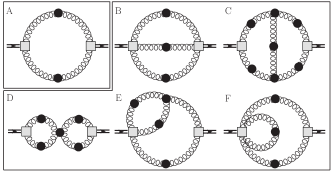
where $\phi=(A,c,\bar{c})$ denotes the expectation value of the fluctuation (super-)field $\hat{\phi}$, e.g. $A=\langle\hat{A}\rangle$, and $G_{\phi_{i}\phi_{j}}=\langle\hat{\phi}_{i}\,\hat{\phi}_{j}\rangle-\langle\hat{\phi}_{i}\rangle\,\langle\hat{\phi}_{j}\rangle$ denotes the propagator of the respective fields. This yields a diagrammatic representation in terms of a finite number of diagrams involving full propagators and vertices, see Fig. 1 for the types of diagrams appearing in the full expansion up to two-loop order. We emphasise that (3) is an exact relation whose finite diagrammatics should not be confused with a perturbative expansion in an infinite series of Feynman diagrams. The internal vertices arise from functional derivatives of the full propagator in (3) and are therefore automatically fully dressed. However, the RG-invariance of the left hand side of (3) only carries over to right hand side if also the external vertices derived from the EMT are dressed with appropriate wave-function renormalisation factors and running couplings. This argument is supported by the flow equation for the EMT itself, which can be derived from the flow equation for composite operators Pawlowski:2005xe , where full vertices are generated during the flow. More heuristically this can also be seen in a skeleton expansion. Therefore, on a diagrammatic level only up to 3-loop diagrams with dressed external vertices appear.

The natural framework for such a calculation is the real-time formalism based on the Schwinger-Keldysh closed time path. Within such a setup one never has to resort to Euclidean field theory. Here one distinguishes two branches of the time contour, conventionally denoted by $+/-$, along with separate fields and sources. Correlation functions thus become matrix valued. In thermal equilibrium the propagator can be parametrised in terms of the spectral function $\rho(\omega,\vec{p})$ only according to

$$G^{\pm\pm}(\omega,\vec{p}) = F(\omega,\vec{p})\pm\text{i}\left(n(\omega)+\tfrac{1}{2}\right)\rho(\omega,\vec{p})\,,$$

$$G^{+-}(\omega,\vec{p}) = -\text{i}\,n(\omega)\rho(\omega,\vec{p})\,,$$

$$G^{-+}(\omega,\vec{p}) = -\text{i}\left(n(\omega)+1\right)\rho(\omega,\vec{p})\,,$$ (4)

where $n(\omega)=1/(\exp(\omega/T)+1)$ denotes the Bose distribution function and $F(\omega,\vec{p})$ is given as a principal value integral,

$$F(\omega,\vec{p})=PV\int\limits_{-\infty}^{\infty}\text{d}\bar{\omega}\,\frac{\rho(\bar{\omega},\vec{p})}{\omega-\bar{\omega}}\,.$$ (5)

The spectral function is defined as

$$\rho(\omega,\vec{p})=G^{-+}(\omega,\vec{p})-G^{+-}(\omega,\vec{p})\,.$$ (6)

Moreover, in thermal equilibrium the KMS relation relates the off-diagonal parts of the propagator via

$$G^{+-}(\omega,\vec{p})=e^{-\beta\omega}G^{-+}(\omega,\vec{p})\,.$$ (7)

Hence we find for the spectral function of the energy momentum tensor

$$\rho_{\pi\pi}(\omega,\vec{p})=(1-e^{-\beta\omega})G^{-+}_{\pi\pi}(\omega,\vec{p})\,.$$ (8)

Inserting the above identity into (1), this implies

$$\eta=-\frac{\beta}{20}G^{-+}_{\pi\pi}(0,0)\,.$$ (9)

Figure 1: Types of diagrams contributing to the correlation function of the energy momentum tensor up to two-loop order; squares denote vertices derived from the EMT; all propagators and vertices are fully dressed.

In this work we present the full two-loop diagrammatics shown in Fig. 1. There are five types of two-loop diagrams arising from the expansion (3): Sunset (B), Maki-Thompson (C), Eight (D), Squint (E), one-loop with vertex correction (F). The branch indices of the external vertices are fixed by (9) as $-+$, whereas we sum over internal branch indices. Thus, unlike in the one-loop case, at two-loop level principal value parts of propagators with equal branch indices can occur. However, at two-loop level possibly divergent contributions can explicitly be shown to cancel due to a left-right symmetry after combining appropriate diagrams. This is no longer true beyond two-loop, where diagrams with divergent sub-diagrams arise.

The only nontrivial input in our calculation, apart from the running coupling $\alpha_{s}$, is the gluon spectral function obtained using MEM from Euclidean FRG data Fister:2011uw . For details about MEM and the properties of the gluon spectral functions we refer the reader to Haas:2013hpa . The running coupling $\alpha_{s}(q,T)$ extracted from the ghost-gluon vertex is calculated from the dressing functions $z_{\bar{c}Ac},Z_{c},Z_{T}$ of the ghost-gluon-vertex, the ghost propagator and the transverse gluon propagator, respectively as

$$\alpha_{s}(q,T)=\frac{z_{\bar{c}Ac}^{2}(q,T)}{4\pi Z_{T}(q,T)Z_{c}(q,T)^{2}}$$ (10)

with data taken from Fister:2011uw . Following the discussion above, all couplings that appear in the vertices are fully dressed running couplings. For each two-loop diagram we study the integrand of the viscosity integral as a function of one of the loop four-momenta $(q_{0},\vec{q})$, integrating out the other one. It turns out that all integrands are peaked in the vicinity of some diagram-dependent value $(q_{0,\rm{max}},\vec{q}_{\rm{max}})$. The running couplings $\alpha_{s}(q,T)$ are then evaluated at a momentum $q_{\mathrm{max}}(T)=\sqrt{q_{0,\rm{max}}^{2}+\vec{q}_{\rm{max}}^{2}}\approx 7\,T$ to minimise the impact of the neglected momentum dependence of the vertices. This implicitly defines a temperature-dependent vertex coupling $\alpha_{s,\text{vert}}(T)=\alpha_{s}(7\,T,T)$.

Results -

Figure 2: Full Yang-Mills result (red) for $\eta/s$ in comparison to lattice results Meyer:2007ic ; Meyer:2009jp (blue) and the AdS/CFT bound (orange). In addition, the plot shows the analytic fit given in (13) and its two components. The ratio $\eta/s$ shows a minimum at $T_{\mathrm{min}}\approx 1.26\,T_{c}$ with a value of 0.14.

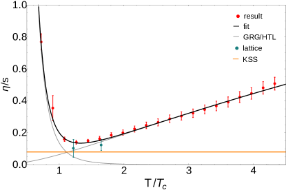
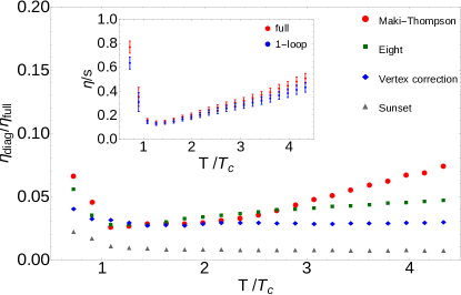
Fig. 2 shows the full two-loop result for $\eta/s$ employing the lattice entropy density from Borsanyi:2012ve including all diagrams from Fig. 1. The data shows, as expected on general grounds, a clear minimum at $T_{\mathrm{min}}\approx 1.26\,T_{c}$. The minimal value $\eta/s(T_{\mathrm{min}})=0.14$ is well above the AdS/CFT bound, where the error bars represent the combined systematic errors from MEM and the FRG calculation. The lattice data Meyer:2007ic ; Meyer:2009jp is in good agreement with our results, supporting the reliability of both methods. The inset in Fig. 3 shows the comparison to the one-loop calculation Haas:2013hpa , illustrating the very good agreement around $T_{c}$. This confirms the argument concerning the optimisation of the RG scheme around $T_{c}$, which was put forward in Haas:2013hpa . Consistent with this reasoning, only at larger temperatures the deviation between the two calculations becomes significant and the relative size of the two-loop contribution grows with temperature. For large temperatures the dominant two-loop contributions arise from the Maki-Thompson and the Eight, see Fig. 3, that resum classes of ladder diagrams. This is consistent with the conventional picture in perturbative expansions where ladder resummations are required to obtain the correct result for the viscosity Jeon:1994if ; Jeon:1995zm . Note that diagrams with overlapping loops are potentially suppressed as the spectral functions are peaked in a narrow region in momentum space. Due to the additional phase space suppression, we expect that diagrams with more than two loops are negligible. We have checked this suppression in a first assessment of three-loop diagrams.

Figure 3: Relative contributions from different diagram types to the two-loop viscosity as a function of temperature. The squint contribution is orders of magnitude smaller and not shown. The inset shows the comparison to the one-loop result Haas:2013hpa .

For understanding the physical picture underlying the temperature behaviour, we provide a global fit function for $\eta/s\,(T)$. Additionally, such an analytic fit function is well-suited for phenomenological applications. This parametrisation has to cover temperature ranges corresponding to vastly different physical situations. At large temperatures $T\gg T_{c}$ the degrees of freedom are gluons which can eventually be treated perturbatively. By contrast, at small temperatures $T\lesssim T_{c}$ YM theory can effectively be described as a glueball resonance gas (GRG). Finally, there is a transition region between these two asymptotic regimes whose description requires non-perturbative techniques.

In the high temperature regime, perturbation theory is applicable and $\eta/s$ is given as a function of the strong coupling $\alpha_{s}$ only. It turns out that the hard-thermal loop (HTL) resummed data Arnold:2003zc is well-described by the functional form

$$\frac{\eta}{s}(\alpha_{s})=\frac{a}{\alpha_{s}^{\gamma}}\,,$$ (11)

with an overall coefficient $a$ and a scaling exponent $\gamma\approx 1.6$. We aim at extracting a non-perturbative extension of the above parametrisation based on our data. In the region $T_{c}-3\,T_{c}$ strong correlations become important and perturbation theory breaks down. This raises the question of a suitable running coupling as there is no unique definition of $\alpha_{s}$ beyond two-loop. A quasi-particle picture suggests that an appropriate choice of $\alpha_{s}$ can be deduced from a heavy quark potential Richardson:1978bt ; Karbstein:2014bsa .

An analytic expression for a coupling that generates a linearly rising static quark potential at large distances is given by Nesterenko:1999np

$$\alpha_{\mbox{\tiny{s,HQ}}}(z)=\frac{1}{\beta_{0}}\frac{z^{2}-1}{z^{2}\log z^{2}}\,,$$ (12)

where $z$ denotes a dimensionless momentum variable. At large momenta it approaches the one-loop running coupling, where $\beta_{0}=33/(12\pi)$ denotes the coefficient in the one-loop beta-function of pure $SU(3)$ Yang-Mills theory. The scale identification is implemented by regarding $\alpha_{\mbox{\tiny{s,HQ}}}$ as a function of $z=c\,T/T_{c}$ with a scale identification factor $c$. By construction, the divergence of (12) at zero momentum leads to a vanishing contribution of (11) to $\eta/s$ at zero temperature. As an estimate for a lower bound for a reasonable high-temperature fit, we consider the trace anomaly as a hint from QCD thermodynamics, which starts to develop a $T^{4}$ behaviour for $T\gtrsim 2\,T_{c}$ Andersen:2011ug . Using $T>3\,T_{c}$ as a conservative estimate, our data is well-described by the scaling form (11) with the running coupling (12) and parameters $a=0.15$ and $c=0.66$. One should note that whereas the heavy quark potential coupling takes a rather large value $\alpha_{\mbox{\tiny{s,HQ}}}(cT/T_{c})|_{T=T_{c}}\approx 1.77$ at $T_{c}$, the vertex coupling $\alpha_{\mbox{\tiny{s,vert}}}(T_{c})\approx 0.76$ corresponding to a value of $\alpha^{\overline{\text{MS}}}_{\mbox{\tiny{s,vert}}}(T_{c})\approx 0.35$, after conversion to the $\overline{\text{MS}}$ scheme vonSmekal:2009ae , is comparably small. This supports the validity of resummation arguments at moderately large temperatures but also underlines the non-uniqueness of the definition of a running coupling in the nonperturbative regime around $T_{c}$. It turns out that the fit (11) can be extended to even lower temperatures $T\gtrsim 1.8T_{c}$, where it is still in very good agreement with our data, see Fig. 2. Note, that the fitting with the vertex coupling $\alpha_{s,\text{vert}}$ fails for temperatures below $3\,T_{c}$. These findings hint at the validity of a quasi-particle picture even at considerably low temperatures.

Below the critical temperature the effective degrees of freedom change from gluons to glueballs. The glueball spectrum can be calculated using the formalism put forward in this work HMP . Hence, the present YM calculation is also capable of describing glueball resonances. Therefore one expects an algebraic decay of $\eta/s$ with temperature similar to a hadron resonance gas Csernai:2006zz ; Hirano:2005wx . Due to the small number of data points and the comparably large error bars below $T_{c}$, no precise determination of the exponent $\delta$ in the power law is possible. We construct a global fit function by superposing a power law behaviour at small temperatures with the extrapolated high temperature behaviour (11), i.e. a global parametrisation of the form

$$\frac{\eta}{s}(T)=\frac{a}{\alpha_{\mbox{\tiny{s,HQ}}}^{\gamma}(c\,T/T_{c})}+\frac{b}{(T/T_{c})^{\delta}}\,.$$ (13)

With $a=0.15$, $b=0.14$, $c=0.66$ and $\delta=5.1$ this fit describes our data very well, see Fig. 2. The best-fit value $\delta=5.1$ lies in the expected range for a hadron resonance gas Hirano:2005wx , where for example a pion gas leads to an exponent of 4.

Figure 4: Estimate for $\eta/s$ in QCD which shows a minimum at $T_{\mathrm{min}}\approx 1.3\,T_{c}$ at a value of $0.17$. The inset shows the comparison to the YM results for temperatures normalised by the respective critical temperatures.

The analytic fit function (13) for $\eta/s$ in YM theory enables us to provide a first estimate of $\eta/s$ in full QCD, again based on the idea of superposing a low and a high temperature behaviour term. The procedure consists of three separate steps. Firstly, one has to take into account the difference in scales and the running couplings in YM and QCD. This involves replacing the coefficient $\beta_{0}$ in (12) by its QCD value, $\beta_{0,\text{\tiny{QCD}}}=(33-2N_{f})/(12\pi)$. Additionally, one has to set a scale by fixing the ratio of the running couplings in YM and QCD at a certain point. In our setup the characteristic scale is the critical temperature $T_{c}$. For the phase transition to the confinement phase to take place, the strong coupling usually needs to exceed a certain critical value $\alpha_{s}(T)=\alpha_{\mathrm{crit}}$. On general grounds one can argue that the critical values in YM theory and QCD are of comparable size. This argument is supported by the fact that the values of $\alpha_{\mathrm{crit}}$ for the vertex couplings tend to coincide. Consequently, we impose the condition

$$\alpha^{N_{f}=0}_{\mbox{\tiny{s,HQ}}}(cT/T_{c})\Bigr{|}_{T=T_{c}}=\alpha^{N_{f}=3}_{\mbox{\tiny{s,HQ}}}(c_{\text{\tiny QCD}}T/T_{c})\Bigr{|}_{T=T_{c}}.$$ (14)

This matching condition fixes the scale factor to the value $c_{\text{\tiny QCD}}=0.79$. Secondly, one has to take into account genuine quark contributions that are not encoded in the change of the running couplings. Denoting the quark contributions to viscosity and entropy as $\Delta\eta$ and $\Delta s$ respectively, we write

$$\begin{split}\frac{\eta}{s}\Bigr{|}_{\text{\tiny{QCD}}}&=\frac{\eta_{\text{\tiny{YM}}}+\Delta\eta}{s_{\text{\tiny{YM}}}+\Delta s}=\frac{\eta}{s}\Bigr{|}_{\text{\tiny{YM}},\alpha^{\text{\tiny YM}}_{s}\to\alpha^{\text{\tiny QCD}}_{s}}\cdot\left(\frac{1+\frac{\Delta\eta}{\eta^{\phantom{YM}}_{\text{YM}}}}{1+\frac{\Delta s}{s^{\phantom{YM}}_{\text{YM}}}}\right),\end{split}$$ (15)

and estimate the ratios $\Delta\eta/\eta_{\text{YM}}$ and $\Delta s/s_{\text{YM}}$ using leading order perturbative results. For $N_{f}=3$ we find $\Delta\eta/\eta_{\text{YM}}\approx 2.9$ Chen:2012jc ; Arnold:2000dr and $\Delta s/s_{\text{YM}}\approx\frac{21}{32}N_{f}\approx 2.0$ Arnold:1994eb ; Andersen:1999va , leading to an overall correction factor of approximately $4/3$. Finally, in the low temperature regime one has to replace the pure glueball resonance gas by a hadron resonance gas, which also decays algebraically with temperature. In this work we use the data given in Demir:2008tr . In summary, the final fit for QCD takes the form (13), but with the parameter $a_{\text{\tiny QCD}}\approx 4/3\,a$ for the high-temperature part and $b_{\text{\tiny QCD}}\approx 0.16$, $\delta_{\text{\tiny QCD}}\approx 5$ for the HRG fit, replacing the corresponding YM values. Additionally the full QCD $\alpha^{N_{f}=3}_{\mbox{\tiny{s,HQ}}}(c_{\text{\tiny QCD}}T/T_{c})$ with $c_{\text{\tiny QCD}}=0.79$ replaces the pure-glue beta-function, whereas the perturbative exponent $\gamma$ remains unchanged. Note that a continuation of the fit to very high energies requires taking into account the quark flavor thresholds appropriately.

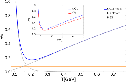
This procedure yields the final result shown in Fig. 4. Plotted in terms of temperatures normalised by the respective critical temperatures, the QCD curve is shifted slightly upwards compared to the YM result, see the inset of Fig. 4. The general shape resembles the one of the YM result and shows a minimum at $T_{\mathrm{min}}\approx 1.3\,T_{c}$ with a value $0.17$.

Summary and Conclusions - We have computed the shear viscosity over entropy density ratio in pure YM theory over a large temperature range. The setup is based on an exact functional relation for the spectral function of the energy-momentum tensor involving full gluon propagators and vertices. The only input are the gluon spectral function and the running coupling $\alpha_{s}$. As a highly non-trivial result, the global temperature behaviour of $\eta/s$ can be described as a direct sum of a glueball resonance gas contribution with an algebraic decay at small temperatures, and a high temperature contribution consistent with HTL-resummed perturbation theory. Finally we provide a first estimate for $\eta/s$ in QCD.

Acknowledgements The authors thank L. McLerran, G. Denicol, H. Niemi, and D. Rischke for discussions. This work is supported by the Helmholtz Alliance HA216/EMMI and the grant ERC-AdG-290623. NC acknowledges funding from the Heidelberg Graduate School of Fundamental Physics.

References

- (1) PHENIX Collaboration, K. Adcox et al., Nucl.Phys. A757, 184 (2005), nucl-ex/0410003.
- (2) STAR Collaboration, J. Adams et al., Nucl.Phys. A757, 102 (2005), nucl-ex/0501009.
- (3) ALICE Collaboration, K. Aamodt et al., Phys.Rev.Lett. 105, 252302 (2010), 1011.3914.
- (4) H. Niemi, G. S. Denicol, P. Huovinen, E. Molnar, and D. H. Rischke, Phys.Rev.Lett. 106, 212302 (2011), 1101.2442.
- (5) L. P. Csernai, J. Kapusta, and L. D. McLerran, Phys.Rev.Lett. 97, 152303 (2006), nucl-th/0604032.
- (6) T. Hirano and M. Gyulassy, Nucl.Phys. A769, 71 (2006), nucl-th/0506049.
- (7) P. Kovtun, D. T. Son, and A. O. Starinets, Phys.Rev.Lett. 94, 111601 (2005), hep-th/0405231.
- (8) U. Heinz and R. Snellings, Ann.Rev.Nucl.Part.Sci. 63, 123 (2013), 1301.2826.
- (9) M. Haas, L. Fister, and J. M. Pawlowski, Phys.Rev. D90, 091501 (2014), 1308.4960.
- (10) G. Aarts and J. M. Martinez Resco, JHEP 0204, 053 (2002), hep-ph/0203177.
- (11) Z. Xu and C. Greiner, Phys.Rev.Lett. 100, 172301 (2008), 0710.5719.
- (12) H. B. Meyer, Phys.Rev. D76, 101701 (2007), 0704.1801.
- (13) H. B. Meyer, Nucl.Phys. A830, 641C (2009), 0907.4095.
- (14) R. Lang and W. Weise, Eur.Phys.J. A50, 63 (2014), 1311.4628.
- (15) R. Marty, E. Bratkovskaya, W. Cassing, J. Aichelin, and H. Berrehrah, Phys.Rev. C88, 045204 (2013), 1305.7180.
- (16) B. A. Gelman, E. V. Shuryak, and I. Zahed, Phys.Rev. A72, 043601 (2005), nucl-th/0410067.
- (17) J. E. Thomas, Nuclear Physics A 830, 665 (2009), 0907.0140.
- (18) T. Schaefer, (2014), 1403.0653.
- (19) R. Kubo, J.Phys.Soc.Jap. 12, 570 (1957).
- (20) K. Kamikado, N. Strodthoff, L. von Smekal, and J. Wambach, Eur.Phys.J. C74, 2806 (2014), 1302.6199.
- (21) S. Strauss, C. S. Fischer, and C. Kellermann, Phys.Rev.Lett. 109, 252001 (2012), 1208.6239.
- (22) J. M. Pawlowski, Annals Phys. 322, 2831 (2007), hep-th/0512261.
- (23) L. Fister and J. M. Pawlowski, (2011), 1112.5440.
- (24) S. Borsanyi, G. Endrodi, Z. Fodor, S. Katz, and K. Szabo, JHEP 1207, 056 (2012), 1204.6184.
- (25) S. Jeon, Phys.Rev. D52, 3591 (1995), hep-ph/9409250.
- (26) S. Jeon and L. G. Yaffe, Phys.Rev. D53, 5799 (1996), hep-ph/9512263.
- (27) P. B. Arnold, G. D. Moore, and L. G. Yaffe, JHEP 0305, 051 (2003), hep-ph/0302165.
- (28) J. L. Richardson, Phys.Lett. B82, 272 (1979).
- (29) F. Karbstein, A. Peters, and M. Wagner, JHEP 1409, 114 (2014), 1407.7503.
- (30) A. Nesterenko, Phys.Rev. D62, 094028 (2000), hep-ph/9912351.
- (31) J. O. Andersen, L. E. Leganger, M. Strickland, and N. Su, Phys.Rev. D84, 087703 (2011), 1106.0514.
- (32) L. von Smekal, K. Maltman, and A. Sternbeck, Phys.Lett. B681, 336 (2009), 0903.1696.
- (33) M. Haas, A. Maas, and J. M. Pawlowski, in preparation (2014).
- (34) J.-W. Chen, Y.-F. Liu, Y.-K. Song, and Q. Wang, Phys.Rev. D87, 036002 (2013), 1212.5308.
- (35) P. B. Arnold, G. D. Moore, and L. G. Yaffe, JHEP 0011, 001 (2000), hep-ph/0010177.
- (36) P. B. Arnold and C.-x. Zhai, Phys.Rev. D51, 1906 (1995), hep-ph/9410360.
- (37) J. O. Andersen, E. Braaten, and M. Strickland, Phys.Rev. D61, 074016 (2000), hep-ph/9908323.
- (38) N. Demir and S. A. Bass, Phys.Rev.Lett. 102, 172302 (2009), 0812.2422.