Signal Recovery on Graphs: Variation Minimization

Abstract

We consider the problem of signal recovery on graphs. Graphs model data with complex structure as signals on a graph. Graph signal recovery recovers one or multiple smooth graph signals from noisy, corrupted, or incomplete measurements. We formulate graph signal recovery as an optimization problem, for which we provide a general solution through the alternating direction methods of multipliers. We show how signal inpainting, matrix completion, robust principal component analysis, and anomaly detection all relate to graph signal recovery and provide corresponding specific solutions and theoretical analysis. We validate the proposed methods on real-world recovery problems, including online blog classification, bridge condition identification, temperature estimation, recommender system for jokes, and expert opinion combination of online blog classification.

I Introduction

With the explosive growth of information and communication, signals are being generated at an unprecedented rate from various sources, including social networks, citation, biological, and physical infrastructures [1, 2]. Unlike time-series or images, these signals have complex, irregular structure, which requires novel processing techniques leading to the emerging field of signal processing on graphs.

Signal processing on graphs extends classical discrete signal processing for time-series to signals with an underlying complex, irregular structure [3, 4, 5, 6]. The framework models that structure by a graph and signals by graph signals, generalizing concepts and tools from classical discrete signal processing to graph signal processing. Recent work involves graph-based filtering [3, 4, 7, 8], graph-based transforms [3, 6, 9], sampling and interpolation on graphs [10, 11, 12], uncertainty principle on graphs [13], semi-supervised classification on graphs [14, 15, 16], graph dictionary learning [17, 18], and community detection on graphs [19]; for a recent review, see [20].

Two basic approaches to signal processing on graphs have been considered, both of which analyze signals with complex, irregular structure, generalizing a series of concepts and tools from classical signal processing, such as graph filters, or graph Fourier transform, to diverse graph-based applications, such as graph signal denoising, compression, classification, and clustering [5, 21, 22, 23]. The first is rooted in spectral graph theory [24, 25] and builds on the graph Laplacian matrix. Since the graph Laplacian matrix is restricted to be symmetric and positive semi-definite, this approach is applicable only to undirected graphs with real and nonnegative edge weights. The second approach, discrete signal processing on graphs ($\mbox{DSP}_{\mbox{\scriptsize G}}$) [3, 4], is rooted in the algebraic signal processing theory [26, 27] and builds on the graph shift operator, which works as the elementary filter that generates all linear shift-invariant filters for signals with a given structure. The graph shift operator is the adjacency matrix and represents the relational dependencies between each pair of nodes. Since the graph shift operator is not restricted to be symmetric, this approach is applicable to arbitrary graphs, those with undirected or directed edges, with real or complex, nonnegative or negative weights.

In this paper, we consider the classical signal processing task of signal recovery within the framework of $\mbox{DSP}_{\mbox{\scriptsize G}}$. Signal recovery problems in the current literature include image denoising [28, 29], signal inpainting [30, 31, 32], and sensing [33, 34], but are limited to signals with regular structure, such as time series. We use $\mbox{DSP}_{\mbox{\scriptsize G}}$ to deal with signals with arbitrary structure, including both undirected and directed graphs. Graph signal recovery attempts to recover one or multiple graph signals that are assumed to be smooth with respect to underlying graphs, from noisy, missing, or corrupted measurements. The smoothness constraint assumes that the signal samples at neighboring vertices are similar [4].

We propose a graph signal model, cast graph signal recovery as an optimization problem, and provide a general solution by using the alternating direction method of multipliers. We show that many classical recovery problems, such as signal inpainting [30, 31, 32], matrix completion [35, 36], and robust principal component analysis [37, 38], are related to the graph signal recovery problem. We propose theoretical solutions and new algorithms for graph signal inpainting, graph signal matrix completion, and anomaly detection of graph signals, all applicable to semi-supervised classification, regression, and matrix completion. Finally, we validate the proposed methods on real-world recovery problems, including online blog classification, bridge condition identification, temperature estimation, recommender system, and expert opinion combination.

Previous work. We now briefly review existing work related to recovery problems. Image denoising recovers an image from noisy observations. Standard techniques include Gaussian smoothing, Wiener local empirical filtering, and wavelet thresholding methods (see [29] and references therein). Signal inpainting reconstructs lost or deteriorated parts of signals, including images and videos. Standard techniques include total variation-based methods [30, 31, 32, 21], image model-based methods [39], and sparse representations [40]. Compressed sensing acquires and reconstructs signals by taking only a limited number of measurements [37, 38]. It assumes that signals are sparse and finds solutions to underdetermined linear systems by $\ell_{1}$ techniques. Matrix completion recovers the entire matrix from a subset of its entries by assuming that the matrix is of low rank. It was originally proposed in [35] and extensions include a noisy version in [36, 41] and decentralized algorithms via graphs [42].  Robust principal component analysis recovers a low-rank matrix from corrupted measurements [37, 38]; it separates an image into two parts: a smooth background and a sparse foreground. In contrast to principal component analysis, it is robust to grossly corrupted entries.

Existing work related to signal recovery based on spectral graph theory includes: 1) interpolation of bandlimited graph signals to recover bandlimited graph signals from a set with specific properties, called the uniqueness set [10, 11]. Extensions include the sampling theorem on graphs [43] and fast distributed algorithms [12]; and 2) smooth regularization on graphs to recover smooth graph signals from random samples [44, 45, 46].

Contributions. The contributions of the paper are as follows:

• a novel algorithm for the general recovery problem that unifies existing algorithms, such as signal inpainting, matrix completion, and robust principal component analysis;

• a novel graph signal inpainting algorithm with analysis of the associated estimation error;

• a novel graph signal matrix completion algorithm with analysis of a theoretical connection between graph total variation and nuclear norm; and

• novel algorithms for anomaly detection of graph signals with analysis of the associated detection accuracy, and for robust graph signal inpainting.

Outline of the paper. Section II formulates the problem and briefly reviews $\mbox{DSP}_{\mbox{\scriptsize G}}$, which lays the foundation for this paper; Section III describes the proposed solution for a graph signal recovery problem. Sections that follow study three subproblems; graph signal inpainting in Section IV, graph signal matrix completion in Section V, and anomaly detection of graph signals in Section VI. Algorithms are evaluated in Section VII on real-world recovery problems, including online blog classification, bridge condition identification, temperature estimation, recommender system for jokes and expert opinion combination. Section VIII concludes the paper and provides pointers to future directions.

II Discrete Signal Processing on Graphs

We briefly review relevant concepts from $\mbox{DSP}_{\mbox{\scriptsize G}}$; for more details, see [3, 4]. $\mbox{DSP}_{\mbox{\scriptsize G}}$ is a theoretical framework that generalizes classical discrete signal processing from regular domains, such as lines and rectangular lattices, to arbitrary, irregular domains commonly represented by graphs, with applications in signal compression, denoising and classification, semi-supervised learning and data recovery [14, 47, 22, 48].

Graph shift. In $\mbox{DSP}_{\mbox{\scriptsize G}}$, signals are represented by a graph $G=(\mathcal{V},\operatorname{A})$, where $\mathcal{V}=\{v_{0},\ldots,v_{N-1}\}$ is the set of nodes, and $\operatorname{A}\in\mathbb{C}^{N\times N}$ is the graph shift, or a weighted adjacency matrix that represents the connections of the graph $G$, either directed or undirected. The $n$th signal element corresponds to the node $v_{n}$, and the edge weight $\operatorname{A}_{n,m}$ between nodes $v_{n}$ and $v_{m}$ is a quantitative expression of the underlying relation between the $n$th and the $m$th signal samples, such as a similarity, a dependency, or a communication pattern.

Graph signal.  Given the graph representation $G=(\mathcal{V},\operatorname{A})$, a graph signal is defined as a map on the graph that assigns the signal samples $x_{n}\in\mathbb{C}$ to the node $v_{n}$. Once the node order is fixed, the graph signal can also be written as a vector

$$\mathbf{x}\ =\ \begin{bmatrix}x_{0},x_{1},\ldots,x_{N-1}\end{bmatrix}^{T}\in\mathbb{C}^{N}.$$ (1)

Graph Fourier transform. In general, a Fourier transform corresponds to the expansion of a signal into basis functions that are invariant to filtering. This invariant basis is the eigenbasis of the graph shift $\operatorname{A}$ (or, if the complete eigenbasis does not exist, the Jordan eigenbasis of $\operatorname{A}$ [3]). For simplicity, assume that $\operatorname{A}$ has a complete eigenbasis, and the spectral decomposition of $\operatorname{A}$ is [49],

$$\operatorname{A}=\operatorname{V}\operatorname{\Lambda}\operatorname{V}^{-1},$$ (2)

where the eigenvectors of $\operatorname{A}$ form the columns of matrix $\operatorname{V}$, and $\operatorname{\Lambda}\in\mathbb{C}^{N\times N}$ is the diagonal matrix of the corresponding eigenvalues $\lambda_{0},\,\lambda_{1},\,\ldots,\,\lambda_{N-1}$ of $\operatorname{A}$. The graph Fourier transform of a graph signal (1) is then

$$\widetilde{\mathbf{x}}=\begin{bmatrix}\widetilde{x}_{0}&\widetilde{x}_{1}&\ldots&\widetilde{x}_{N-1}\end{bmatrix}^{T}=\operatorname{V}^{-1}\mathbf{x},$$ (3)

where $\widetilde{x}_{n}$ in (3) represents the signal’s expansion in the eigenvector basis and forms the frequency content of the graph signal $\mathbf{x}$. The inverse graph Fourier transform reconstructs the graph signal from its frequency content by combining the graph frequency components weighted by the coefficients of the signal’s graph Fourier transform,

$$\mathbf{x}=\operatorname{V}\widetilde{\mathbf{x}}.$$

Variation on graphs. Signal smoothness is a qualitative characteristic that expresses how much signal samples vary with respect to the underlying signal representation domain. To quantify it, $\mbox{DSP}_{\mbox{\scriptsize G}}$ uses the graph total variation based on the $\ell_{p}$-norm [4],

$$\operatorname{S}_{p}(\mathbf{x})=\left|\left|\mathbf{x}-\frac{1}{|\lambda_{\max}{(\operatorname{A})}|}\operatorname{A}\mathbf{x}\right|\right|_{p}^{p},$$ (4)

where $\lambda_{\max}{(\operatorname{A})}$ denotes the eigenvalue of $\operatorname{A}$ with the largest magnitude. We normalize the graph shift to guarantee that the shifted signal is properly scaled with respect to the original one. When $p=2$, we call (4) the quadratic form of graph total variation.

We summarize the notation in Table I.

Symbol	Description	Dimension
$\mathbf{x}$	graph signal	$N$
$\operatorname{X}$	matrix of graph signal	$N\times L$
$\operatorname{A}$	graph shift	$N\times N$
$\widetilde{\operatorname{A}}$	$(\operatorname{I}-\operatorname{A})^{*}(\operatorname{I}-\operatorname{A})$	$N\times N$
$\mathcal{M}$	accessible indices
$\mathcal{U}$	inaccessible indices
$\mathbf{x}_{\mathcal{M}}$	accessible elements in $\mathbf{x}$
$\operatorname{X}_{\mathcal{M}}$	accessible elements in $\operatorname{X}$
$\operatorname{\Theta}(\cdot)$	element-wise shrinkage function defined in (14)
$\mathcal{D}(\cdot)$	singular-value shrinkage function defined in (15)

TABLE I: Key notation used in the paper.

III Graph Signal Recovery

We now formulate the general recovery problem for graph signals to unify multiple signal completion and denoising problems and generalize them to arbitrary graphs. In the sections that follow, we consider specific cases of the graph signal recovery problem, propose appropriate solutions, and discuss their implementations and properties.

Let $\mathbf{x}^{(\ell)}\in\mathbb{C}^{N}$, $1\leq\ell\leq L$, be graph signals residing on the graph $G=(\mathcal{V},\operatorname{A})$, and let $\operatorname{X}$ be the $N\times L$ matrix of graph signals,

$$\operatorname{X}=\begin{bmatrix}\mathbf{x}^{(1)}&\mathbf{x}^{(2)}&\ldots&\mathbf{x}^{(L)}\end{bmatrix}.$$ (5)

Assume that we do not know these signals exactly, but for each signal we have a corresponding measurement $\mathbf{t}^{(\ell)}$. Since each $\mathbf{t}^{(\ell)}$ can be corrupted by noise and outliers, we consider the $N\times L$ matrix of measurements to be

$$\operatorname{T}=\begin{bmatrix}\mathbf{t}^{(1)}&\mathbf{t}^{(2)}&\ldots&\mathbf{t}^{(L)}\end{bmatrix}=\operatorname{X}+\operatorname{W}+\operatorname{E},$$ (6)

where matrices $\operatorname{W}$ and $\operatorname{E}$ contain noise and outliers, respectively. Note that an outlier is an observation point that is distant from other observations, which may be due to variability in the measurement. We assume that the noise coefficients in $\operatorname{W}$ have small magnitudes, i.e., they can be upper-bounded by a small value, and that the matrix $\operatorname{E}$ is sparse, containing few non-zero coefficients of large magnitude. Furthermore, when certain nodes on a large graph are not accessible, the measurement $\mathbf{t}^{(\ell)}$ may be incomplete. To reflect this, we denote the sets of indices of accessible and inaccessible nodes as $\mathcal{M}$ and $\mathcal{U}$, respectively. Note that inaccessible nodes denote that values on those nodes are far from the ground-truth because of corruption, or because we do not have access to them.

Signal recovery from inaccessible measurements requires additional knowledge of signal properties. In this work, we make the following assumptions: (a) the signals of interest $\mathbf{x}^{(\ell)}$, are smooth with respect to the representation graph $G=(\mathcal{V},\operatorname{A})$; we express this by requiring that the variation of recovered signals be small; (b) since the signals of interest $\mathbf{x}^{(\ell)}$ are all supported on the same graph structure, we assume that these graph signals are similar and provide redundant information; we express this by requiring that the matrix of graph signals $\operatorname{X}$ has low rank; (c) the outliers happen with a small probability; we express this by requiring that the matrix $\operatorname{E}$ be sparse; and (d) the noise has small magnitude; we express this by requiring that the matrix $\operatorname{W}$ be upper-bounded. We thus formulate the problem as follows:

$$\widehat{\operatorname{X}},\widehat{\operatorname{W}},\widehat{\operatorname{E}} = \arg\min_{\operatorname{X},\operatorname{W},\operatorname{E}}\ \alpha\operatorname{S}_{2}(\operatorname{X})+\beta~{}{\rm rank}(\operatorname{X})+\gamma\left\|\operatorname{E}\right\|_{0},$$

subject to $$\left\|\operatorname{W}\right\|_{F}^{2}~{}\leq~{}\epsilon^{2},$$ (9)

$$\operatorname{T}_{\mathcal{M}}=(\operatorname{X}+\operatorname{W}+\operatorname{E})_{\mathcal{M}},$$

where $\widehat{\operatorname{X}},\widehat{\operatorname{W}},\widehat{\operatorname{E}}$ denote the optimal solutions of the graph signal matrix, the noise matrix, and the outlier matrix, respectively, $\epsilon$ controls the noise level, $\alpha,\beta,\gamma$ are tuning parameters, and

$$\operatorname{S}_{2}(\operatorname{X}) = \sum_{\ell=1}^{L}{\operatorname{S}_{2}(\mathbf{x}^{(\ell)})}=\left\|\operatorname{X}-\operatorname{A}\operatorname{X}\right\|_{F}^{2},$$ (10)

where $\left\|\cdot\right\|_{F}$ denotes the Frobenius norm and represents the cumulative quadratic form of the graph total variation (4) for all graph signals, and $\left\|\operatorname{E}\right\|_{0}$ is the $\ell_{0}$-norm that is defined as the number of nonzero entries in $\operatorname{E}$. The general problem (III) recovers the graph signal matrix (5) from the noisy measurements (6), possibly when only a subset of nodes is accessible.

Instead of using the graph total variation based on $\ell_{1}$ norm [4], we use the quadratic form of the graph total variation (4) for two reasons. First, it is computationally easier to optimize than the $\ell_{1}$-norm based graph total variation. Second, the $\ell_{1}$-norm based graph total variation, which penalizes less transient changes than the quadratic form, is good at separating smooth from non-smooth parts of graph signals; the goal here, however, is to force graph signals at each node to be smooth. We thus use the quadratic form of the graph total variation in this paper and, by a slight abuse of notation, call it graph total variation for simplicity.

The minimization problem (III) with conditions (9) and (9) reflects all of the above assumptions: (a) minimizing the graph total variation $\operatorname{S}_{2}(\operatorname{X})$ forces the recovered signals to be smooth and to lie in the subspace of “low” graph frequencies [4]; (b) minimizing the rank of $\operatorname{X}$ forces the graph signals to be similar and provides redundant information; (c) minimizing the $\ell_{0}$-norm $\left\|\operatorname{E}\right\|_{0}$ forces the outlier matrix to have few non-zero coefficients; (d) condition (9) captures the assumption that the coefficients of $\operatorname{W}$ have small magnitudes; and (e) condition (9) ensures that the solution coincides with the measurements on the accessible nodes.

Unfortunately, solving (III) is hard because of the rank and the $\ell_{0}$-norm [50, 51]. To solve it efficiently, we relax and reformulate (III) as follows:

$$\widehat{\operatorname{X}},\widehat{\operatorname{W}},\widehat{\operatorname{E}} = \arg\min_{\operatorname{X},\operatorname{W},\operatorname{E}}\ \alpha\operatorname{S}_{2}(\operatorname{X})+\beta\left\|\operatorname{X}\right\|_{*}+\gamma\left\|\operatorname{E}\right\|_{1},$$

subject to $$\left\|\operatorname{W}\right\|_{F}^{2}~{}\leq~{}\epsilon^{2},$$ (13)

$$\operatorname{T}_{\mathcal{M}}=(\operatorname{X}+\operatorname{W}+\operatorname{E})_{\mathcal{M}}.$$

In (LABEL:eq:C_Opt), we replace the rank of $\operatorname{X}$ with the nuclear norm, $\left\|\operatorname{X}\right\|_{*}$, defined as the sum of all the singular values of $\operatorname{X}$, which still promotes low rank [35, 36]. We further replace the $\ell_{0}$-norm of $\operatorname{E}$ with the $\ell_{1}$-norm, which still promotes sparsity of $\operatorname{E}$ [50, 51]. The minimization problems (III) and (LABEL:eq:C_Opt) follow the same assumptions and promote the same properties, but (III) is an ideal version, while (LABEL:eq:C_Opt) is a practically feasible version, because it is a convex problem and thus easier to solve. We call (LABEL:eq:C_Opt) the graph signal recovery (GSR) problem; see Table II.

To solve (LABEL:eq:C_Opt) efficiently, we use the alternating direction method of multipliers (ADMM) [52]. ADMM is an algorithm that is intended to take advantage of both the decomposability and the superior convergence properties of the method of multipliers. In ADMM, we first formulate an augmented function and then iteratively update each variable in an alternating or sequential fashion, ensuring the convergence of the method [52]. We leave the derivation to the Appendix, and summarize the implementation in Algorithm 1.

Algorithm 1 Graph Signal Recovery

Input	$\operatorname{T}$     matrix of measurements
Output	$\widehat{\operatorname{X}}$     matrix of graph signals
	$\widehat{\operatorname{W}}$    matrix of outliers
	$\widehat{\operatorname{E}}$     matrix of noise
Function	GSR($\operatorname{T}$)
	while the stopping criterion is not satisfied
	while the stopping criterion is not satisfied
	$\operatorname{X}\leftarrow\mathcal{D}_{\beta\eta^{-1}}{\left(\operatorname{X}+t(\operatorname{T}-\operatorname{W}-\operatorname{E}-\operatorname{C}-\eta^{-1}(\operatorname{Y}_{1}+\operatorname{Y}_{2})-\operatorname{Z})\right)}$
	end
	$\operatorname{W}\leftarrow\eta(\operatorname{T}-\operatorname{X}-\operatorname{E}-\operatorname{C}-\eta^{-1}\operatorname{Y}_{1})/(\eta+2)$
	while the stopping criterion is not satisfied
	$\operatorname{E}\leftarrow\operatorname{\Theta}_{\gamma\eta^{-1}}{\left(\operatorname{X}+t(\operatorname{T}-\operatorname{X}-\operatorname{W}-\operatorname{C}-\eta^{-1}\operatorname{Y}_{1})\right)}$
	end
	$\operatorname{Z}\leftarrow(\operatorname{I}+2\alpha\eta^{-1}(\operatorname{I}-\operatorname{A})^{*}(\operatorname{I}-\operatorname{A}))^{-1}(\operatorname{X}-\eta^{-1}\operatorname{Y}_{2})$
	$\operatorname{C}_{\mathcal{M}}\leftarrow 0,\operatorname{C}_{\mathcal{U}}\leftarrow(\operatorname{T}-\operatorname{X}-\operatorname{W}-\operatorname{E}-\eta^{-1}\operatorname{Y}_{1})_{\mathcal{U}}$,
	$\operatorname{Y}_{1}\leftarrow\operatorname{Y}_{1}-\eta(\operatorname{T}-\operatorname{X}-\operatorname{W}-\operatorname{E}-\operatorname{C})$
	$\operatorname{Y}_{2}\leftarrow\operatorname{Y}_{2}-\eta(\operatorname{X}-\operatorname{Z})$
	end
	return $\widehat{\operatorname{X}}\leftarrow\operatorname{X},~{}\widehat{\operatorname{W}}\leftarrow\operatorname{W},~{}\widehat{\operatorname{E}}\leftarrow\operatorname{E}$

Note that in Algorithm 1, $\operatorname{Y}_{1},\operatorname{Y}_{2}$ are Lagrangian multipliers, $\eta$ is pre-defined, the step size $t$ is chosen from backtracking line search [53], and operators $\operatorname{\Theta}_{\tau}$ and $\mathcal{D}_{\tau}$ are defined for $\tau\geq 0$ as follows: $\operatorname{\Theta}_{\tau}(\operatorname{X})$ “shrinks” every element of $\operatorname{X}$ by $\tau$ so that the $(n,m)$th element of $\operatorname{\Theta}_{\tau}(\operatorname{X})$ is

$$\operatorname{\Theta}_{\tau}(\operatorname{X})_{n,m}=\begin{cases}\operatorname{X}_{n,m}-\tau,&\text{when \,\,\,}\operatorname{X}_{n,m}\geq\tau,\\ \operatorname{X}_{n,m}+\tau,&\text{when \,\,\,}\operatorname{X}_{n,m}\leq-\tau,\\ 0,&\text{otherwise}.\end{cases}$$ (14)

Similarly, $\mathcal{D}_{\tau}(\operatorname{X})$ “shrinks” the singular values of $\operatorname{X}$,

$$\mathcal{D}_{\tau}(\operatorname{X})=\operatorname{U}\operatorname{\Theta}_{\tau}{(\Sigma)}\operatorname{Q}^{*},$$ (15)

where $\operatorname{X}=\operatorname{U}\Sigma\operatorname{Q}^{*}$ denotes the singular value decomposition of $\operatorname{X}$ [49] and $*$ denotes the Hermitian transpose. The following stopping criterion is used in the paper: the difference of the objective function between two consecutive iterations is smaller than $10^{-8}$. The bulk of the computational cost is in the singular value decomposition (15) when updating $\operatorname{X}$, which is also involved in the standard implementation of matrix completion.

We now review several well-known algorithms for signal recovery, including signal inpainting, matrix completion, and robust principal component analysis, and show how they can be formulated as special cases of the graph signal recovery problem (III). In Sections IV and V, we show graph counterparts of the signal inpainting and matrix completion problems by minimizing the graph total variation. In Section VI, we show anomaly detection on graphs, which is inspired by robust principal component analysis.

Signal inpainting. Signal inpainting is a process of recovering inaccessible or corrupted signal samples from accessible samples using regularization [30, 31, 32, 21], that is, minimization of the signal’s total variation. The measurement is typically modeled as

$$\mathbf{t}=\mathbf{x}+\mathbf{w}\in\mathbb{R}^{N},$$ (16)

where $\mathbf{x}$ is the true signal, and $\mathbf{w}$ is the noise. Assuming we can access a subset of indices, denoted as $\mathcal{M}$, the task is then to recover the entire true signal $\mathbf{x}$, based on the accessible measurement $\mathbf{t}_{\mathcal{M}}$. We assume that the true signal $\mathbf{x}$ is smooth, that is, its variation is small. The variation is expressed by a total variation function

$$\operatorname{TV}{(\mathbf{x})}\ =\ \sum_{i=1}^{N}|x_{i}-x_{i-1~{}{\rm mod}~{}N}|.$$ (17)

We then recover the signal $\mathbf{x}$ by solving the following optimization problem:

$$\widehat{\mathbf{x}} = \arg\min_{\mathbf{x}}\,\operatorname{TV}(\mathbf{x}),$$ (18)

subject to $$\left\|(\mathbf{x}-\mathbf{t})_{\mathcal{M}}\right\|_{2}^{2}~{}\leq~{}\epsilon^{2}.$$ (19)

The condition (19) controls how well the accessible measurements are preserved. As discussed in Section II, both the $\ell_{1}$ norm based graph total variation and the quadratic form of the graph total variation (4) are used. Thus, (18) is a special case of (LABEL:eq:C_Opt) when the graph shift is the cyclic permutation matrix, $\alpha=1$, $L=1$, $\beta=\gamma=0$, $\operatorname{E}=0$, and conditions (13) and (13) are combined into the single condition (19); see Table II.

Matrix completion. Matrix completion recovers a matrix given a subset of its elements, usually, a subset of rows or columns. Typically, the matrix has a low rank, and the missing part is recovered through rank minimization [35, 36, 41]. The matrix is modeled as

$$\operatorname{T}=\operatorname{X}+\operatorname{W}\in\mathbb{R}^{N\times L},$$ (20)

where $\operatorname{X}$ is the true matrix and $\operatorname{W}$ is the noise. Assuming we can access a subset of indices, denoted as $\mathcal{M}$, the matrix $\operatorname{X}$ is recovered from (20) as the solution with the lowest rank:

$$\widehat{\operatorname{X}} = \arg\min_{\operatorname{X}}\,\left\|\operatorname{X}\right\|_{*},$$ (21)

subject to $$\left\|(\operatorname{X}-\operatorname{T})_{\mathcal{M}}\right\|_{2}^{2}~{}\leq~{}\epsilon^{2};$$ (22)

this is a special case of (LABEL:eq:C_Opt) with $\alpha=\gamma=0$, $\beta=1$, $\operatorname{E}=0$, and conditions (13) and (13) are combined into the single condition (22); see Table II. This also means that the values in the matrix are associated with a graph that is represented by the identity matrix, that is, we do not have any prior information about the graph structure.

Robust principal component analysis. Similarly to matrix completion, robust principal component analysis is used for recovering low-rank matrices. The main difference is the assumption that all matrix elements are measurable but corrupted by outliers [37, 38]. In this setting, the matrix is modeled as

$$\operatorname{T}=\operatorname{X}+\operatorname{E}\in\mathbb{R}^{N\times L},$$ (23)

where $\operatorname{X}$ is the true matrix, and $\operatorname{E}$ is a sparse matrix of outliers.

The matrix $\operatorname{X}$ is recovered from (23) as the solution with the lowest rank and fewest outliers:

$$\widehat{\operatorname{X}},\widehat{\operatorname{E}} = \arg\min_{\operatorname{X},\operatorname{E}}\,\beta\left\|{\operatorname{X}}\right\|_{*}+\gamma\left\|\operatorname{E}\right\|_{1},$$

subject to $$\operatorname{T}=\operatorname{X}+\operatorname{E};$$

this is a special case of (LABEL:eq:C_Opt) with $\alpha=\epsilon=0$, $\operatorname{W}=0$, and $\mathcal{M}$ contains all the indices; see Table II. Like before, this also means that the matrix is associated with a graph that is represented by the identity matrix, that is, we do not have any prior information about the graph structure.

IV Graph Signal Inpainting

We now discuss in detail the problem of signal inpainting on graphs. Parts of this section have appeared in [47], and we include them here for completeness.

As discussed in Section III, signal inpainting (18) seeks to recover the missing entries of the signal $\mathbf{x}$ from incomplete and noisy measurements under the assumption that two consecutive signal samples in $\mathbf{x}$ have similar values. Here, we treat $\mathbf{x}$ as a graph signal that is smooth with respect to the corresponding graph. We thus update the signal inpainting problem (18), and formulate the graph signal inpainting problem as

$$\widehat{\mathbf{x}} = \arg\min_{\mathbf{x}}\,\operatorname{S}_{2}(\mathbf{x}),$$ (24)

subject to $$\left\|(\mathbf{x}-\mathbf{t})_{\mathcal{M}}\right\|_{2}^{2}~{}\leq~{}\epsilon^{2};$$ (25)

this is a special case of (LABEL:eq:C_Opt) with $L=1,\beta=\gamma=0$; see Table II.

Solutions. In general, graph signal inpainting (24) can be solved by using Algorithm 1. However, in special cases, there exist closed-form solutions that do not require iterative algorithms.

IV-1 Noiseless inpainting

Suppose that the measurement $\mathbf{t}$ in (16) does not contain noise. In this case, $\mathbf{w}=0$, and we solve (24) for $\epsilon=0$:

$$\widehat{\mathbf{x}} = \arg\min_{\mathbf{x}}\,\operatorname{S}_{2}(\mathbf{x}),$$ (26)

subject to $$\mathbf{x}_{\mathcal{M}}=\mathbf{t}_{\mathcal{M}}.$$

We call the problem (26) graph signal inpainting via total variation minimization (GTVM) [47].

Let $\widetilde{\operatorname{A}}=(\operatorname{I}-\operatorname{A})^{*}(\operatorname{I}-\operatorname{A})$. By reordering nodes, write $\widetilde{\operatorname{A}}$ in block form as

$$\widetilde{\operatorname{A}}=\begin{bmatrix}\widetilde{\operatorname{A}}_{\mathcal{M}\mathcal{M}}&\widetilde{\operatorname{A}}_{\mathcal{M}\mathcal{U}}\\ \widetilde{\operatorname{A}}_{\mathcal{U}\mathcal{M}}&\widetilde{\operatorname{A}}_{\mathcal{U}\mathcal{U}}\end{bmatrix},$$

and set the derivative of (26) to $0$; the closed-form solution is

$$\widehat{\mathbf{x}}=\begin{bmatrix}\mathbf{t}_{\mathcal{M}}\\ -\widetilde{\operatorname{A}}_{\mathcal{U}\mathcal{U}}^{-1}\widetilde{\operatorname{A}}_{\mathcal{U}\mathcal{M}}\mathbf{t}_{\mathcal{M}}\end{bmatrix}.$$

When $\widetilde{\operatorname{A}}_{\mathcal{U}\mathcal{U}}$ is not invertible, a pseudoinverse should be used.

IV-2 Unconstrained inpainting

The graph signal inpainting (24) can be formulated as an unconstrained problem by merging condition (25) with the objective function:

$$\widehat{\mathbf{x}}=\arg\min_{\mathbf{x}}\,\left\|(\mathbf{x}-\mathbf{t})_{\mathcal{M}}\right\|_{2}^{2}+\alpha\operatorname{S}_{2}(\mathbf{x}),$$ (27)

where the tuning parameter $\alpha$ controls the trade-off between the two parts of the objective function. We call (27) the graph signal inpainting via total variation regularization (GTVR). GTVR is a convex quadratic problem that has a closed-form solution. Setting the derivative of (27) to zero, we obtain the closed-form solution

$$\widehat{\mathbf{x}}=\left(\begin{bmatrix}\operatorname{I}_{\mathcal{M}\mathcal{M}}&0\\ 0&0\end{bmatrix}+\alpha\widetilde{\operatorname{A}}\right)^{-1}\begin{bmatrix}\mathbf{t}_{\mathcal{M}}\\ \operatorname{\mathbf{0}}\end{bmatrix},$$

where $\operatorname{I}_{\mathcal{M}\mathcal{M}}$ is an identity matrix. When the term in parentheses is not invertible, a pseudoinverse should be adopted.

Theoretical analysis. Let $\mathbf{x}^{0}$ denote the true graph signal that we are trying to recover. Assume that $\operatorname{S}_{2}{(\mathbf{x}^{0})}=\eta^{2}$ and $\mathbf{x}^{0}$ satisfies (25), so that $\left\|\mathbf{x}^{0}_{\mathcal{M}}-\mathbf{t}_{\mathcal{M}}\right\|_{2}^{2}~{}\leq~{}\epsilon^{2}.$ Similarly to (IV-1), we write $\operatorname{A}$ in a block form as

$${\operatorname{A}}\ =\ \begin{bmatrix}{\operatorname{A}}_{\mathcal{M}\mathcal{M}}&{\operatorname{A}}_{\mathcal{M}\mathcal{U}}\\ {\operatorname{A}}_{\mathcal{U}\mathcal{M}}&{\operatorname{A}}_{\mathcal{U}\mathcal{U}}\end{bmatrix}.$$

The following results, proven in [47], establish an upper bound on the error of the solution to graph signal inpainting (24).

Lemma 1.

The error $\left\|\mathbf{x}^{0}-\widehat{\mathbf{x}}\right\|_{2}$ of the solution $\widehat{\mathbf{x}}$ to the graph signal inpainting problem (24) is bounded as

$$\left\|\mathbf{x}^{0}-\widehat{\mathbf{x}}\right\|_{2} \leq \frac{q}{2}\left\|(\mathbf{x}^{0}-\widehat{\mathbf{x}})_{\mathcal{U}}\right\|_{2}+p|\epsilon|+|\eta|,$$

where

$$p=\left|\left|\begin{bmatrix}\operatorname{I}_{\mathcal{M}\mathcal{M}}+\operatorname{A}_{\mathcal{M}\mathcal{M}}\\ \operatorname{A}_{\mathcal{U}\mathcal{M}}\end{bmatrix}\right|\right|_{2},\,\,\,q=\left|\left|\begin{bmatrix}\operatorname{A}_{\mathcal{M}\mathcal{U}}\\ \operatorname{I}_{\mathcal{U}\mathcal{U}}+\operatorname{A}_{\mathcal{U}\mathcal{U}}\end{bmatrix}\right|\right|_{2},$$

and $\left\|\cdot\right\|_{2}$ for matrices denotes the spectral norm.

Theorem 1.

If $q<2$, then the error on the inaccessible part of the solution $\widehat{\mathbf{x}}$ is bounded as

$$\left\|(\mathbf{x}^{0}-\widehat{\mathbf{x}})_{\mathcal{U}}\right\|_{2} \leq \frac{2p|\epsilon|+2|\eta|}{2-q}.$$

The condition $q<2$ may not hold for some matrices; however, if $\operatorname{A}$ is symmetric, we have $q~{}\leq~{}\left\|\operatorname{I}+\operatorname{A}\right\|_{2}$ $~{}\leq~{}\left\|\operatorname{I}\right\|_{2}+\left\|\operatorname{A}\right\|_{2}=2$, since $\left\|\operatorname{A}\right\|_{2}=1$. Since $q$ is related to the size of the inaccessible part, when we take a larger number of measurements, $q$ becomes smaller, which leads to a tighter upper bound. Also, note that the upper bound is related to the smoothness of the true graph signal and the noise level of the accessible part. A central assumption of any inpainting technique is that the true signal $\mathbf{x}^{0}$ is smooth. If this assumption does not hold, then the upper bound is large and useless. When the noise level of the accessible part is smaller, the measurements from the accessible part are closer to the true values, which leads to a smaller estimation error.

V Graph Signal Matrix Completion

We now consider graph signal matrix completion—another important subproblem of the general graph signal recovery problem (III).

As discussed in Section III, matrix completion seeks to recover missing entries of matrix $\operatorname{X}$ from the incomplete and noisy measurement matrix (20) under the assumption that $\operatorname{X}$ has low rank. Since we view $\operatorname{X}$ as a matrix of graph signals (see (5)), we also assume that the columns of $\operatorname{X}$ are smooth graph signals. In this case, we update the matrix completion problem (21) and formulate the graph signal matrix completion problem as

$$\widehat{\operatorname{X}} = \arg\min_{\operatorname{X}}\,\operatorname{S}_{2}(\operatorname{X})+\beta\left\|\operatorname{X}\right\|_{*},$$ (28)

subject to $$\left\|(\operatorname{X}-\operatorname{T})_{\mathcal{M}}\right\|_{F}^{2}~{}\leq~{}\epsilon^{2};$$

this is a special case of (LABEL:eq:C_Opt) with $\alpha=1,\gamma=0$; see Table II.

Solutions. In addition to Algorithm 1 that can be used to solve the graph signal matrix completion problem (28), there exist alternative approaches that we discuss next.

V-1 Minimization

Here we consider the noise-free case. Suppose the measurement matrix $\operatorname{T}$ in (20) does not contain noise. We thus solve (28) for $\operatorname{W}=0$ and $\epsilon=0$,

$$\widehat{\operatorname{X}} = \arg\min_{\operatorname{X}}\,\operatorname{S}_{2}(\operatorname{X})+\beta\left\|\operatorname{X}\right\|_{*},$$ (29)

subject to $$\operatorname{X}_{\mathcal{M}}=\operatorname{T}_{\mathcal{M}}.$$

We call (29) graph signal matrix completion via total variation minimization (GMCM). This is a constrained convex problem that can be solved by projected generalized gradient descent [53]. We first split the objective function into two components, a convex, differential component, and a convex, nondifferential component; based on these two components, we formulate a proximity function and then solve it iteratively. In each iteration, we solve the proximity function with an updated input and project the result onto the feasible set. To be more specific, we split the objective function (29) into a convex, differentiable component $\operatorname{S}_{2}(\operatorname{X})$, and a convex, nondifferential component $\beta\left\|\operatorname{X}\right\|_{*}$. The proximity function is then defined as

$$\operatorname{prox}_{t}(\operatorname{X}) = \arg\min_{\operatorname{Z}}\frac{1}{2t}\left\|\operatorname{X}-\operatorname{Z}\right\|^{2}+\beta\left\|\operatorname{X}\right\|_{*}$$

$$= \mathcal{D}_{t\beta}(\operatorname{Z}),$$

where $\mathcal{D}(\cdot)$ is defined in (15). In each iteration, we first solve for the proximity function and project the result onto the feasible set as

$$\operatorname{X}\leftarrow{\operatorname{proj}}\left(\operatorname{prox}_{t}\left(\operatorname{X}-t\nabla\operatorname{S}_{2}(\operatorname{X})\right)\right),$$

where $t$ is the step size that is chosen from the backtracking line search [53], and $\operatorname{proj}(\operatorname{X})$ projects $\operatorname{X}$ to the feasible set so that the $(n,m)$th element of $\operatorname{proj}(\operatorname{X})$ is

$$\operatorname{proj}(\operatorname{X})_{n,m}=\begin{cases}\operatorname{T}_{n,m},&\text{when \,\,\,}(n,m)\in\mathcal{M},\\ \operatorname{X}_{n,m},&\text{when \,\,\,}(n,m)\in\mathcal{U}.\\ \end{cases}$$

For implementation details, see Algorithm 2. The bulk of the computational cost of Algorithm 2 is in the singular value decomposition (15) when updating $\operatorname{X}$, which is also involved in the standard implementation of matrix completion.

Algorithm 2 Graph Signal Matrix Completion via Total Variation Minimization

Input	$\operatorname{T}$     matrix of measurements
	$\widehat{\operatorname{X}}$     matrix of graph signals
Function	GMCM($\operatorname{T}$)
	initialize $\operatorname{X}$, such that $\operatorname{X}_{\mathcal{M}}=\operatorname{T}_{\mathcal{M}}$ holds
	while the stopping criterion is not satisfied
	Choose step size $t$ from backtracking line search
	$\operatorname{X}\leftarrow\operatorname{proj}\left(\mathcal{D}_{t\beta}(\operatorname{X}-2t\widetilde{\operatorname{A}}\operatorname{X})\right)$
	end
	return $\widehat{\operatorname{X}}\leftarrow\operatorname{X}$

V-2 Regularization

The graph signal matrix completion (28) can be formulated as an unconstrained problem,

$$\noindent\widehat{\operatorname{X}} = \arg\min_{\operatorname{X}}\,\left\|\operatorname{X}_{\mathcal{M}}-\operatorname{T}_{\mathcal{M}}\right\|_{F}^{2}+\alpha\operatorname{S}_{2}(\operatorname{X})+\beta\left\|\operatorname{X}\right\|_{*}.$$ (30)

We call (30) graph signal matrix completion via total variation regularization (GMCR). This is an unconstrained convex problem and can be solved by generalized gradient descent. Similarly to projected generalized gradient descent, generalized gradient descent also formulates and solves a proximity function. The only difference is that generalized gradient descent does not need to project the result after each iteration to a feasible set. To be more specific, we split the objective funtion (29) into a convex, differentiable component $\left\|\operatorname{X}_{\mathcal{M}}-\operatorname{T}_{\mathcal{M}}\right\|_{F}^{2}+\alpha\operatorname{S}_{2}(\operatorname{X})$, and a convex, non-differential component $\beta\left\|\operatorname{X}\right\|_{*}$. The proximity function is then defined as

$$\operatorname{prox}_{t}(\operatorname{X}) = \arg\min_{\operatorname{Z}}\frac{1}{2t}\left\|\operatorname{X}-\operatorname{Z}\right\|^{2}+\beta\left\|\operatorname{X}\right\|_{*}$$ (31)

$$= \mathcal{D}_{t\beta}(\operatorname{Z}),$$

where $\mathcal{D}(\cdot)$ is defined in (15). In each iteration, we first solve for the proximity function as

$$\operatorname{X}\leftarrow\operatorname{prox}_{t}\left(\operatorname{X}-t\nabla\left(\left\|\operatorname{X}_{\mathcal{M}}-\operatorname{T}_{\mathcal{M}}\right\|_{F}^{2}+\alpha\operatorname{S}_{2}(\operatorname{X})\right)\right),$$ (32)

where $t$ is the step size that is chosen from the backtracking line search [53]; for implementation details, see Algorithm 3.

Algorithm 3 Graph Signal Matrix Completion via Total Variation Regularization

Input	$\operatorname{T}$    matrix of measurements
	$\widehat{\operatorname{X}}$    matrix of graph signals
Function	GMCR($\operatorname{T}$)
	initialize $\operatorname{X}$
	while the stopping criterion is not satisfied
	Choose step size $t$ from backtracking line search
	$\operatorname{X}\leftarrow\mathcal{D}_{t\beta}\left(\operatorname{X}-2t(\operatorname{X}_{\mathcal{M}}-\operatorname{T}_{\mathcal{M}})-2\alpha t\widetilde{\operatorname{A}}\operatorname{X}\right)$
	end
	return $\widehat{\operatorname{X}}\leftarrow\operatorname{X}$

The bulk of the computational cost of Algorithm 3 is in the singular value decomposition (15) when updating $\operatorname{X}$, which is also involved in the standard implementation of matrix completion.

Theoretical analysis. We now discuss properties of the proposed algorithms. The key in classical matrix completion is to minimize the nuclear norm of a matrix. Instead of considering general matrices, we only focus on graph signal matrices, whose corresponding algorithm is to minimize both the graph total variation and the nuclear norm. We study the connection between graph total variation and nuclear norm of a matrix to reveal the underlying mechanism of our algorithm.

Let $\operatorname{X}$ be a $N\times L$ matrix of rank $r$ with singular value decomposition $\operatorname{X}=\operatorname{U}\Sigma\operatorname{Q}^{*}$, where $\operatorname{U}=\begin{bmatrix}\mathbf{u}_{1}&\mathbf{u}_{2}&\ldots&\mathbf{u}_{r}\end{bmatrix}$, $\operatorname{Q}=\begin{bmatrix}\mathbf{q}_{1}&\mathbf{q}_{2}&\ldots&\mathbf{q}_{r}\end{bmatrix}$, and $\Sigma$ is a diagonal matrix with $\sigma_{i}$ along the diagonal, $i=1,\cdots,r$.

Lemma 2.

$$\operatorname{S}_{2}(\operatorname{X})=\sum_{i=1}^{r}{\sigma_{i}^{2}\left\|(\operatorname{I}-\operatorname{A})\mathbf{u}_{i}\right\|_{2}^{2}}.$$

Proof.

$$\operatorname{S}_{2}(\operatorname{X}) = \left\|\operatorname{X}-\operatorname{A}\operatorname{X}\right\|_{F}^{2}\ \stackrel{{\scriptstyle(a)}}{{=}}\ \left\|(\operatorname{I}-\operatorname{A})\operatorname{U}\Sigma\operatorname{Q}^{*}\right\|_{F}^{2},$$

$$= {\rm Tr}\Biggl{(}\operatorname{Q}\Sigma\operatorname{U}^{*}(\operatorname{I}-\operatorname{A})^{*}(\operatorname{I}-\operatorname{A})\operatorname{U}\Sigma\operatorname{Q}^{*}\Biggr{)},$$

$$\stackrel{{\scriptstyle(b)}}{{=}} {\rm Tr}\Biggl{(}\Sigma\operatorname{U}^{*}(\operatorname{I}-\operatorname{A})^{*}(\operatorname{I}-\operatorname{A})\operatorname{U}\Sigma\operatorname{Q}^{*}\operatorname{Q}\Biggr{)},$$

$${=} \left\|(\operatorname{I}-\operatorname{A})\operatorname{U}\Sigma\right\|_{F}^{2}\ \stackrel{{\scriptstyle(c)}}{{=}}\ \sum_{i=1}^{r}{\sigma_{i}^{2}\left\|(\operatorname{I}-\operatorname{A})\mathbf{u}_{i}\right\|_{2}^{2}},$$

where $(a)$ follows from the singular value decomposition; $(b)$ from the cyclic property of the trace operator; and $(c)$ from $\Sigma$ being a diagonal matrix. ∎

From Lemma 2, we see that graph total variation is related to the rank of $\operatorname{X}$; in other words, lower rank naturally leads to smaller graph total variation.

Theorem 2.

$$\operatorname{S}_{2}(\operatorname{X})\leq\operatorname{S}_{2}(\operatorname{U})\left\|\operatorname{X}\right\|_{*}^{2}.$$

Proof.

From Lemma 2, we have

$$\operatorname{S}_{2}(\operatorname{X}) {=} \left\|(\operatorname{I}-\operatorname{A})\operatorname{U}\Sigma\right\|_{F}^{2}\ \stackrel{{\scriptstyle(a)}}{{\leq}}\ \left\|(\operatorname{I}-\operatorname{A})\operatorname{U}\right\|_{F}^{2}\left\|\Sigma\right\|_{F}^{2},$$

$$\stackrel{{\scriptstyle(b)}}{{\leq}} \left\|(\operatorname{I}-\operatorname{A})\operatorname{U}\right\|_{F}^{2}\left\|\Sigma\right\|_{*}^{2}\ {=}\ \left\|\operatorname{U}-\operatorname{A}\operatorname{U}\right\|_{F}^{2}\left\|\operatorname{X}\right\|_{*}^{2},$$

where $(a)$ follows from the submultiplicativity of the Frobenius norm; and $(b)$ from the norm equivalence [49]. ∎

In Theorem 2, we see that the graph total variation is related to two quantities: the nuclear norm of $\operatorname{X}$ and the graph total variation of the left singular vectors of $\operatorname{X}$. The first quantity reveals that minimizing the nuclear norm potentially leads to minimizing the graph total variation. We can thus rewrite the objective function (28) as

$$\operatorname{S}_{2}(\operatorname{X})+\beta\left\|\operatorname{X}\right\|_{*} \leq \operatorname{S}_{2}(\operatorname{U})\left\|\operatorname{X}\right\|_{*}^{2}+\beta\left\|\operatorname{X}\right\|_{*}.$$

If the graph shift is built from insufficient information, we just choose a larger $\beta$ to force the nuclear norm to be small, which causes a small graph total variation in return. The quantity $\operatorname{S}_{2}(\operatorname{U})$ measures the smoothness of the left singular vectors of $\operatorname{X}$ on a graph shift $\operatorname{A}$; in other words, when the left singular vectors are smooth, the graph signal matrix is also smooth. We can further use this quantity to bound the graph total variation of all graph signals that belong to a subspace spanned by the left singular vectors.

Theorem 3.

Let a graph signal $\mathbf{x}$ belong to the space spanned by $\operatorname{U}$, that is, $\mathbf{x}=\operatorname{U}\mathbf{a}$, where $\mathbf{a}$ is the vector of representation coefficients. Then,

$$\operatorname{S}_{2}(\mathbf{x})\leq\operatorname{S}_{2}(\operatorname{U})\left\|\mathbf{a}\right\|_{2}^{2}$$

Proof.

$$\operatorname{S}_{2}(\mathbf{x}) = \left\|\mathbf{x}-\operatorname{A}\mathbf{x}\right\|_{2}^{2}\ =\ \left\|(\operatorname{I}-\operatorname{A})\operatorname{U}\mathbf{a}\right\|_{2}^{2}$$

$$\stackrel{{\scriptstyle(a)}}{{\leq}} \left\|(\operatorname{I}-\operatorname{A})\operatorname{U}\right\|_{2}^{2}\left\|\mathbf{a}\right\|_{2}^{2}\ \stackrel{{\scriptstyle(b)}}{{\leq}}\ \left\|(\operatorname{I}-\operatorname{A})\operatorname{U}\right\|_{F}^{2}\left\|\mathbf{a}\right\|_{2}^{2}.$$

where (a) follows from the submultiplicativity of the spectral norm; and (b) from the norm equivalence [49]. ∎

Theorem 3 shows that a graph signal is smooth when it belongs to a subspace spanned by the smooth left singular vectors.

Graph signal recovery problem	$\widehat{\operatorname{X}},\widehat{\operatorname{W}},\widehat{\operatorname{E}}=\arg\min_{\operatorname{X},\operatorname{W},\operatorname{E}\in\mathbb{R}^{N\times L}}\ \alpha\operatorname{S}_{2}(\operatorname{X})+\beta\left\|\operatorname{X}\right\|_{*}+\gamma\left\|\operatorname{E}\right\|_{1},$
	subject to $\left\|\operatorname{W}\right\|_{F}^{2}~{}\leq~{}\epsilon^{2},\operatorname{T}_{\mathcal{M}}=(\operatorname{X}+\operatorname{W}+\operatorname{E})_{\mathcal{M}}.$
Signal inpainting	$L=1,\beta=0,\gamma=0,$ graph shift is the cyclic permutation matrix.
Matrix completion	$\alpha=0$, or graph shift is the identity matrix, $\gamma=0$
Robust principal component analysis	$\alpha=0$, or graph shift is the identity matrix, $\epsilon=0,\mathcal{M}$ is all the indices in $\operatorname{T}$.
Graph signal inpainting	$L=1,\beta=0,\gamma=0$
Graph signal matrix completion	$\alpha=1,\gamma=0$
Anomaly detection	$L=1,\beta=0,\mathcal{M}$ is all indices in $\operatorname{T}$
Robust graph signal inpainting	$L=1,\beta=0$

TABLE II: The table of algorithms.

VI Anomaly Detection

We now consider anomaly detection of graph signals, another important subproblem of the general recovery problem (III).

As discussed in Section III, robust principal component analysis seeks to detect outlier coefficients from a low-rank matrix. Here, anomaly detection of graph signals seeks to detect outlier coefficients from a smooth graph signal. We assume that the outlier is sparse and contains few non-zero coefficients of large magnitude. To be specific, the measurement is modeled as

$$\mathbf{t}=\mathbf{x}+\mathbf{e}\in\mathbb{R}^{N},$$ (33)

where $\mathbf{x}$ is a smooth graph signal that we seek to recover, and the outlier $\mathbf{e}$ is sparse and has large magnitude on few nonzero coefficients. The task is to detect the outlier $\mathbf{e}$ from the measurement $\mathbf{t}$. Assuming that $\mathbf{x}$ is smooth, that is, its variation is small, and $\mathbf{e}$ is sparse, we propose the ideal optimization problem as follows:

$$\widehat{\mathbf{x}},\widehat{\mathbf{e}} = \arg\min_{\mathbf{x},\mathbf{e}}\,\left\|\mathbf{e}\right\|_{0}$$ (34)

subject to $$\operatorname{S}_{2}(\mathbf{x})\leq\eta^{2},$$

$$\mathbf{t}=\mathbf{x}+\mathbf{e}.$$

To solve it efficiently, instead of dealing with the $\ell_{0}$ norm, we relax it to the $\ell_{1}$ norm and reformulate (34) as follows:

$$\widehat{\mathbf{x}},\widehat{\mathbf{e}} = \arg\min_{\mathbf{x},\mathbf{e}}\,\left\|\mathbf{e}\right\|_{1}$$ (35)

subject to $$\operatorname{S}_{2}(\mathbf{x})\leq\eta^{2},$$ (37)

$$\mathbf{t}=\mathbf{x}+\mathbf{e};$$

this is a special case of (LABEL:eq:C_Opt) with $L=1,\beta=0,\mathcal{M}$ contains all indices in $\mathbf{t}$, and choosing $\alpha$ properly to ensure that (VI) holds, see Table II. In Section 4, we show that, under these assumptions, both (34) and (35) lead to perfect outlier detection.

Solutions. The minimization problem (35) is convex, and it is numerically efficient to solve for its optimal solution.

We further formulate an unconstrained problem as follows:

$$\widehat{\mathbf{e}} = \arg\min_{\mathbf{e}}\,\operatorname{S}_{2}(\mathbf{t}-\mathbf{e})+\beta\left\|\mathbf{e}\right\|_{1}.$$ (38)

We call (38) anomaly detection via $\ell_{1}$ regularization (AD). In (38), we merge conditions (37) and (37) and move them from the constraint to the objective function. We solve (38) by using generalized gradient descent, as discussed in Section V. For implementation details, see Algorithm 4.

Algorithm 4 Anomaly detection via $\ell_{1}$ regularization

Input	$\mathbf{t}$   input graph signals
Output	$\widehat{\mathbf{e}}$   outlier signals
Function	AD$(\mathbf{x})$
	initialize $\mathbf{e}$
	while the stopping criterion is not satisfied
	Choose step size $t$ from backtracking line search
	$\mathbf{e}\leftarrow\operatorname{\Theta}_{t\beta}\left(\mathbf{e}-2t\widetilde{\operatorname{A}}(\mathbf{t}-\mathbf{e})\right)$
	end
	return $\widehat{\mathbf{e}}\leftarrow\mathbf{e}$

Theoretical analysis. Let $\mathbf{x}^{0}$ be the true graph signal, represented as $\mathbf{x}^{0}=\operatorname{V}\mathbf{a}^{0}=\sum_{i=0}^{N-1}{a_{i}^{0}\mathbf{v}_{i}}$, where $\operatorname{V}$ is defined in (2), $\mathbf{e}^{0}$ be the outliers that we are trying to detect, represented as $\mathbf{e}^{0}=\sum_{i\in\mathcal{E}}{b_{i}\boldsymbol{\delta}_{i}}$, where $\boldsymbol{\delta}_{i}$ is impulse on the $i$th node, and $\mathcal{E}$ contains the outlier indices, that is, $\mathcal{E}\subset\{0,1,2,\cdots N-1\}$, and $\mathbf{t}=\mathbf{x}^{0}+\mathbf{e}^{0}$ be the measurement.

Lemma 3.

Let $\widehat{\mathbf{x}},\widehat{\mathbf{e}}$ be the solution of  (34), and let $\widehat{\mathbf{x}}=\operatorname{V}\widehat{\mathbf{a}}=\sum_{i=0}^{N-1}{\widehat{a}_{i}\mathbf{v}_{i}}$. Then,

$$\widehat{\mathbf{e}}=\operatorname{V}(\mathbf{a}^{0}-\widehat{\mathbf{a}})+\sum_{i\in\mathcal{E}}{b_{i}\boldsymbol{\delta}_{i}}.$$

Proof.

$$\widehat{\mathbf{e}}\ \stackrel{{\scriptstyle(a)}}{{=}}\ \mathbf{t}-\widehat{\mathbf{x}}\ \stackrel{{\scriptstyle(b)}}{{=}}\ \mathbf{x}^{0}+\mathbf{e}^{0}-\widehat{\mathbf{x}}\ \stackrel{{\scriptstyle(c)}}{{=}}\ \operatorname{V}\mathbf{a}^{0}+\sum_{i\in\mathcal{E}}{b_{i}\boldsymbol{\delta}_{i}}-\operatorname{V}\widehat{\mathbf{a}},$$

where $(a)$ follows from the feasibility of $\widehat{\mathbf{x}},\widehat{\mathbf{e}}$ in (LABEL:eq:AD_Opt_cond_2); $(b)$ from the definition of $\mathbf{t}$; and $(c)$ from the definitions of $\mathbf{x}^{0}$ and $\widehat{\mathbf{x}}$. ∎

Lemma 3 provides another representation of the outliers, which is useful in the following theorem.

Let $\operatorname{K}=(\operatorname{I}-\Lambda)^{T}\operatorname{V}^{T}\operatorname{V}(\operatorname{I}-\Lambda)$, the $\operatorname{K}$ norm as $\left\|\mathbf{x}\right\|_{\operatorname{K}}=\sqrt{\mathbf{x}^{T}\operatorname{K}\mathbf{x}}$, and $\mathcal{K}_{\eta}=\{\mathbf{a}\in\mathbb{R}^{N}:\left\|\mathbf{a}\right\|_{\operatorname{K}}\leq\eta,{\rm for~{}all~{}}\mathbf{a}\neq 0\}$.

Lemma 4.

Let  $\mathbf{x}=\operatorname{V}\mathbf{a}$ satisfy (37), (37), and $\mathbf{a}\neq 0$. Then, $\mathbf{a}\in\mathcal{K}_{\eta}$.

Proof.

$$\operatorname{S}_{2}(\mathbf{x}) = \left\|\mathbf{x}-\operatorname{A}\mathbf{x}\right\|_{2}^{2}\ {=}\ \left\|\operatorname{V}\mathbf{a}-\operatorname{A}\operatorname{V}\mathbf{a}\right\|_{2}^{2},$$

$$\stackrel{{\scriptstyle(a)}}{{=}} \left\|\operatorname{V}\mathbf{a}-\operatorname{V}\Lambda\mathbf{a}\right\|_{2}^{2}\ {=}\ \mathbf{a}^{T}(\operatorname{I}-\Lambda)^{T}\operatorname{V}^{T}\operatorname{V}(\operatorname{I}-\Lambda)\mathbf{a},$$

$$\stackrel{{\scriptstyle(b)}}{{=}} \mathbf{a}^{T}\operatorname{K}\mathbf{a}\ \stackrel{{\scriptstyle(c)}}{{\leq}}\ \eta^{2},$$

where $(a)$ follows from (2); $(b)$ from the definition of the $\operatorname{K}$ norm; and $(c)$ from the feasibility of $\mathbf{x}$. ∎

Lemma 4 shows that the frequency components of the solution from (34) and (35) belong to a subspace, which is useful in the following theorem.

Theorem 4.

Let $\operatorname{S}_{2}(\mathbf{x}^{0})\leq\eta^{2}$, $\mathbf{x}^{0}\neq 0$, $\left\|\mathbf{e}^{0}\right\|_{0}\leq k$, and $\widehat{\mathbf{x}},\widehat{\mathbf{e}}$ be the solution of (34) with $\widehat{\mathbf{x}}\neq 0$. Let $\mathcal{K}_{2\eta}$ have the following property:

$$\left\|\operatorname{V}\mathbf{a}\right\|_{0}\geq 2k+1~{}~{}~{}~{}~{}{\rm for~{}all~{}}\mathbf{a}\in\mathcal{K}_{2\eta},$$

where $k\geq\left\|\mathbf{e}^{0}\right\|_{0}$. Then, perfect recovery is achieved,

$$\widehat{\mathbf{x}}\ =\ \mathbf{x}^{0},\widehat{\mathbf{e}}\ =\ \mathbf{e}^{0}.$$

Proof.

Since both $\mathbf{x}^{0}=\operatorname{V}\mathbf{a}^{0}$ and $\widehat{\mathbf{x}}=\operatorname{V}\widehat{\mathbf{a}}$ are feasible solutions of  (34), by Lemma 4, we then have that $\mathbf{a}^{0},\widehat{\mathbf{a}}\in\mathcal{K}_{\eta}$. We next bound their difference, $\mathbf{a}^{0}-\widehat{\mathbf{a}}$, by the triangle inequality, as $\left\|\mathbf{a}^{0}-\widehat{\mathbf{a}}\right\|_{\operatorname{K}}\leq\left\|\mathbf{a}^{0}\right\|_{\operatorname{K}}+\left\|\widehat{\mathbf{a}}\right\|_{\operatorname{K}}\leq 2\eta$.

If $\mathbf{a}^{0}\neq\widehat{\mathbf{a}}$, then $\mathbf{a}^{0}-\widehat{\mathbf{a}}\in\mathcal{K}_{2\eta}$, so that $\left\|\operatorname{V}(\mathbf{a}^{0}-\widehat{\mathbf{a}})\right\|_{0}\geq 2k+1$. From Lemma 3, we have $\left\|\widehat{\mathbf{e}}\right\|_{0}=\left\|\operatorname{V}(\mathbf{a}^{0}-\widehat{\mathbf{a}})+\sum_{i\in\mathcal{E}}{b_{i}\mathbf{e}_{i}}\right\|_{0}\geq k+1$. The last inequality comes from the fact that at most $k$ indices can be canceled by the summation.

On the other hand, $\widehat{\mathbf{e}}$ is the optimum of (34), thus, $\left\|\widehat{\mathbf{e}}\right\|_{0}\leq\left\|\mathbf{e}^{0}\right\|_{0}=k$, which leads to a contradiction.

Therefore, $\widehat{\mathbf{a}}=\mathbf{a}^{0}$ and $\widehat{\mathbf{e}}=\mathbf{e}^{0}$. ∎

Theorem 4 shows the condition that leads to perfect outlier detection by following (34). The key is that the outliers are sufficiently sparse and the smooth graph signal is not sparse.

Theorem 5.

Let $\operatorname{S}_{2}(\mathbf{x}^{0})\leq\eta^{2}$, $\mathbf{x}^{0}\neq 0$, $\left\|\mathbf{e}^{0}\right\|_{0}\leq k$, and $\widehat{\mathbf{x}},\widehat{\mathbf{e}}$ be the solution of (35) with $\widehat{\mathbf{x}}\neq 0$. Let $\mathcal{K}_{2\eta}$ have the following property:

$$\left\|\left(\operatorname{V}\mathbf{a}\right)_{\mathcal{E}^{c}}\right\|_{1}>\left\|\left(\operatorname{V}\mathbf{a}\right)_{\mathcal{E}}\right\|_{1}~{}~{}~{}~{}~{}{\rm for~{}all~{}}\mathbf{a}\in\mathcal{K}_{2\eta}$$

where $\mathcal{E}^{c}\cap\mathcal{E}$ is the empty set, $\mathcal{E}^{c}\cup\mathcal{E}=\{0,1,2,\cdots N-1\}$. Then, perfect recovery is achieved,

$$\widehat{\mathbf{x}}\ =\ \mathbf{x}^{0},\widehat{\mathbf{e}}\ =\ \mathbf{e}^{0}.$$

Proof.

From Lemma 3, we have

$$\left\|\widehat{\mathbf{e}}\right\|_{1} = \left\|\operatorname{V}(\mathbf{a}^{0}-\widehat{\mathbf{a}})+\sum_{i\in\mathcal{E}}{b_{i}\boldsymbol{\delta}_{i}}\right\|_{1}$$

$$= \left\|\left(\operatorname{V}(\mathbf{a}^{0}-\widehat{\mathbf{a}})\right)_{\mathcal{E}^{c}}+\left(\operatorname{V}(\mathbf{a}^{0}-\widehat{\mathbf{a}})\right)_{\mathcal{E}}+\sum_{i\in\mathcal{E}}{b_{i}\boldsymbol{\delta}_{i}}\right\|_{1}$$

$$= \left\|\left(\operatorname{V}(\mathbf{a}^{0}-\widehat{\mathbf{a}})\right)_{\mathcal{E}^{c}}\right\|_{1}+\left\|\left(\operatorname{V}(\mathbf{a}^{0}-\widehat{\mathbf{a}})\right)_{\mathcal{E}}+\sum_{i\in\mathcal{E}}{b_{i}\boldsymbol{\delta}_{i}}\right\|_{1}$$

Denote $\left(\operatorname{V}(\mathbf{a}^{0}-\widehat{\mathbf{a}})\right)_{\mathcal{E}}=\sum_{i\in\mathcal{E}}{d_{i}\boldsymbol{\delta}_{i}}$, we further have

$$\left\|\widehat{\mathbf{e}}\right\|_{1} = \left\|\left(\operatorname{V}(\mathbf{a}^{0}-\widehat{\mathbf{a}})\right)_{\mathcal{E}^{c}}\right\|_{1}+\left\|\sum_{i\in\mathcal{E}}{(d_{i}+b_{i})\boldsymbol{\delta}_{i}}\right\|_{1}$$

$$= \left\|\left(\operatorname{V}(\mathbf{a}^{0}-\widehat{\mathbf{a}})\right)_{\mathcal{E}^{c}}\right\|_{1}+\sum_{i\in\mathcal{E}}|d_{i}+b_{i}|$$

If $\mathbf{a}^{0}\neq\widehat{\mathbf{a}}$, then $\mathbf{a}^{0}-\widehat{\mathbf{a}}\in\mathcal{K}_{2\eta}$. By the assumption, we have $\left\|\left(\operatorname{V}(\mathbf{a}^{0}-\widehat{\mathbf{a}})\right)_{\mathcal{E}^{c}}\right\|_{1}>\left\|\left(\operatorname{V}(\mathbf{a}^{0}-\widehat{\mathbf{a}})\right)_{\mathcal{E}}\right\|_{1}=\left\|\sum_{i\in\mathcal{E}}{d_{i}\boldsymbol{\delta}_{i}}\right\|_{1}=\sum_{i\in\mathcal{E}}|d_{i}|$. We thus obtain

$$\left\|\widehat{\mathbf{e}}\right\|_{1} = \left\|\left(\operatorname{V}(\mathbf{a}^{0}-\widehat{\mathbf{a}})\right)_{\mathcal{E}^{c}}\right\|_{1}+\sum_{i\in\mathcal{E}}|d_{i}+b_{i}|$$

$$> \sum_{i\in\mathcal{E}}(|d_{i}|+|d_{i}+b_{i}|)\ \geq\ \sum_{i\in\mathcal{E}}|b_{i}|.$$

On the other hand, $\widehat{\mathbf{e}}$ is the optimum of (35), so $\left\|\widehat{\mathbf{e}}\right\|_{1}\leq\left\|\mathbf{e}^{0}\right\|_{1}=\left\|\sum_{i\in\mathcal{E}}{b_{i}\boldsymbol{\delta}_{i}}\right\|_{1}=\sum_{i\in\mathcal{E}}|b_{i}|$, which leads to a contradiction.

Therefore, $\widehat{\mathbf{a}}=\mathbf{a}^{0}$ and $\widehat{\mathbf{e}}=\mathbf{e}^{0}$. ∎

Theorems 4 and 5 show that under appropriate assumptions, (34),  (35) detects the outliers perfectly. Note that the assumptions on $\mathcal{K}$ in Theorems 4 and 5 are related to two factors: the upper bound on smoothness, $\eta$, and the eigenvector matrix, $\operatorname{V}$. The volume of $\mathcal{K}_{2\eta}$ is determined by the upper bound on smoothness, $\eta$. The mapping properties of $\operatorname{V}$ are also restricted by Theorems 4 and 5. For instance, in Theorem 4, the eigenvector matrix should map each element in $\mathcal{K}_{2\eta}$ to a non-sparse vector.

Robust graph signal inpainting. One problem with the graph signal inpainting in Section IV is that it tends to trust the accessible part, which may contain sparse, but large-magnitude outliers. Robust graph signal inpainting should prevent the solution from being influenced by the outliers. We thus consider the following optimization problem:

$$\widehat{\mathbf{x}},\widehat{\mathbf{w}},\widehat{\mathbf{e}} = \arg\min_{\mathbf{x},\mathbf{w},\mathbf{e}}\ \alpha\operatorname{S}_{2}(\mathbf{x})+\gamma\left\|\mathbf{e}\right\|_{0},$$ (39)

subject to $$\left\|\mathbf{w}\right\|_{F}^{2}<\eta^{2}$$ (41)

$$\mathbf{t}_{\mathcal{M}}=(\mathbf{x}+\mathbf{w}+\mathbf{e})_{\mathcal{M}};$$

this is a special case of (III) with $L=1,\beta=0$; see Table II.

Similarly to (LABEL:eq:C_Opt), instead of dealing with the $\ell_{0}$ norm, we relax it to be the $\ell_{1}$ norm and reformulate (39) as an unconstrained problem,

$$\widehat{\mathbf{x}},\widehat{\mathbf{e}}\ =\ \arg\min_{\mathbf{x},\mathbf{e}}\,\left\|\mathbf{t}_{\mathcal{M}}-(\mathbf{x}+\mathbf{e})_{\mathcal{M}}\right\|^{2}+\alpha\operatorname{S}_{2}(\mathbf{x})+\gamma\left\|\mathbf{e}\right\|_{1}.$$ (42)

We call problem (42) the robust graph total variation regularization (RGTVR) problem. In (42), we merge conditions (41) and (41) and move them from the constraint to the objective function. Note that (42) combines anomaly detection and graph signal inpainting to provide a twofold inpainting. The first level detects the outliers in the accessible part and provides a clean version of the accessible measurement; the second level uses the clean measurement to recover the inaccessible part. We solve (42) by using ADMM, as discussed in Section III. For implementation details, see Algorithm 5.

Algorithm 5 Robust Graph Total Variation Regularization

Input	$\mathbf{t}$   input graph signal
Output	$\widehat{\mathbf{e}}$   outlier graph signal
	$\widehat{\mathbf{x}}$   output graph signal
Function	RGTVR($\mathbf{t}$)
	while the stopping criterion is not satisfied
	$\mathbf{x}\leftarrow\left(\operatorname{I}+2\alpha\eta^{-1}\widetilde{\operatorname{A}}\right)^{-1}(\mathbf{t}-\mathbf{e}-\mathbf{w}-\mathbf{c}-\eta^{-1}\lambda)$
	$\mathbf{w}\leftarrow\eta{(\mathbf{t}-\mathbf{x}-\mathbf{w}-\mathbf{c}-\eta^{-1}\lambda)}/(\eta+2)$
	$\mathbf{e}\leftarrow\operatorname{\Theta}_{\gamma\eta^{-1}}{(\mathbf{t}-\mathbf{x}-\mathbf{e}-\mathbf{c}-\eta^{-1}\lambda)}$
	$\lambda\leftarrow\lambda-\eta(\mathbf{t}-\mathbf{x}-\mathbf{e}-\mathbf{w}-\mathbf{c})$
	$\mathbf{c}_{\mathcal{M}}\leftarrow 0,\mathbf{c}_{\mathcal{U}}\leftarrow(\mathbf{t}-\mathbf{x}-\mathbf{w}-\mathbf{e}-\eta^{-1}{\lambda})_{\mathcal{U}}$,
	end
	return $\widehat{\mathbf{e}}\leftarrow\mathbf{e},~{}~{}\widehat{\mathbf{x}}\leftarrow\mathbf{x}$

VII Experimental Results

We now evaluate the proposed methods on several real-world recovery problems. Further, we apply graph signal inpainting and robust graph signal inpainting to online blog classification and bridge condition identification for indirect bridge structural health monitoring; We apply graph signal matrix completion to temperature estimation and expert opinion combination.

Datasets. We use the following datasets in the experiments:

VII-1 Online blogs

We consider the problem of classifying $N=1224$ online political blogs as either conservative or liberal [55]. We represent conservative labels as $+1$ and liberal ones as $-1$. The blogs are represented by a graph in which nodes represent blogs, and directed graph edges correspond to hyperlink references between blogs. For a node $v_{n}$, its outgoing edges have weights $1/\deg(v_{n})$, where $\deg(v_{n})$ is the out-degree of $v_{n}$ (the number of outgoing edges). The graph signal here is the label assigned to the blogs.

VII-2 Acceleration signals

We next consider the bridge condition identification problem [56, 57]. To validate the feasibility of indirect bridge structural health monitoring, a lab-scale bridge-vehicle dynamic system was built. Accelerometers were installed on a vehicle that travels across the bridge; acceleration signals were then collected from those accelerometers. To simulate the severity of different bridge conditions on a lab-scale bridge, masses with various weights were put on the bridge. We collected 30 acceleration signals for each of 31 mass levels from 0 to 150 grams in steps of 5 grams, to simulate different degrees of damages, for a total of 930 acceleration signals. For more details on this dataset, see [58].

The recordings are represented by an $8$-nearest neighbor graph, in which nodes represent recordings, and each node is connected to eight other nodes that represent the most similar recordings. The graph signal here is the mass level over all the acceleration signals. The graph shift $\operatorname{A}$ is formed as $\operatorname{A}_{i,j}=\operatorname{P}_{i,j}/\sum_{i}{\operatorname{P}_{i,j}}$, with

$$\operatorname{P}_{i,j}\ =\ \exp\left(\frac{-N^{2}\left\|\mathbf{f}_{i}-\mathbf{f}_{j}\right\|_{2}}{\sum_{i,j}\left\|\mathbf{f}_{i}-\mathbf{f}_{j}\right\|_{2}}\right),$$

and $\mathbf{f}_{i}$ is a vector representation of the features of the $i$th recording. Note that $\operatorname{P}$ is a symmetric matrix that represents an undirected graph and the graph shift $\operatorname{A}$ is an asymmetric matrix that represents a directed graph, which is allowed by the framework of $\mbox{DSP}_{\mbox{\scriptsize G}}$. From the empirical performance, we find that a directed graph provides much better results than an undirected graph.

VII-3 Temperature data

We consider 150 weather stations in the United States that record their local temperatures [3]. Each weather station has 365 days of recordings (one recording per day), for a total of 54,750 measurements. The graph representing these weather stations is obtained by measuring the geodesic distance between each pair of weather stations. The nodes are represented by an $8$-nearest neighbor graph, in which nodes represent weather stations, and each node is connected to eight other nodes that represent the eight closest weather stations. The graph signals here are the temperature values recorded in each weather station.

The graph shift $\operatorname{A}$ is formed as $\operatorname{A}_{i,j}=\operatorname{P}_{i,j}/\sum_{i}{\operatorname{P}_{i,j}}$, with

$$\operatorname{P}_{i,j}=\exp\left(-\frac{N^{2}d_{i,j}}{\sum_{i,j}{d_{i,j}}}\right),$$

where $d_{i,j}$ is the geodesic distance between the $i$th and the $j$th weather stations. Similarly to the acceleration signals, we normalize $\operatorname{P}$ to obtain a asymmetric graph shift, which represents a directed graph, to achieve better empirical performance.

VII-4 Jester dataset 1

The Jester joke data set [59] contains $4.1\times 10^{6}$ ratings of 100 jokes from 73,421 users. The graph representing the users is obtained by measuring the $\ell_{1}$ norm of existing ratings between each pair of jokes. The nodes are represented by an 8-nearest neighbor graph in which nodes represent users and each node is connected to eight other nodes that represent similar users. The graph signals are the ratings of each user. The graph shift $\operatorname{A}$ is formed as

$$\operatorname{P}_{i,j}\ =\ \exp\left(\frac{-N^{2}\left\|\mathbf{f}_{i}-\mathbf{f}_{j}\right\|_{1}}{\sum_{i,j}\left\|\mathbf{f}_{i}-\mathbf{f}_{j}\right\|_{1}}\right),$$

where $\mathbf{f}_{i}$ is the vector representation of the existing ratings for the $i$th user. Similarly to acceleration signals, we normalize $\operatorname{P}$ to obtain an asymmetric graph shift, which represents a directed graph, to achieve better empirical performance.

Evaluation score. To evaluate the performance of the algorithms, we use the following four metrics: accuracy (ACC), mean square error (MSE), root mean square error (RMSE), and mean absolute error (MAE), defined as

$${\rm ACC} \ =\ \frac{1}{N}\sum_{i=1}^{N}{\bf 1}{(x_{i}=\widehat{x}_{i})},$$

$${\rm MSE} \ =\ \frac{1}{N}\sum_{i=1}^{N}{(x_{i}-\widehat{x}_{i})^{2}},$$

$${\rm RMSE} \ =\ \sqrt{\frac{1}{N}\sum_{i=1}^{N}{(x_{i}-\widehat{x}_{i})^{2}}}=\sqrt{{\rm MSE}},$$

$${\rm MAE} \ =\ \frac{\sum_{i=1}^{N}{|x_{i}-\widehat{x}_{i}|}}{N},$$

where $x_{i}$ is the ground-truth for the $i$th sample, $\widehat{x}_{i}$ is the estimate for the $i$th sample, and ${\bf 1}$ is the indicator function, ${\bf 1}(x)=1$, for $x=0$, and $0$ otherwise.

In the following applications, the tuning parameters for each algorithm are chosen by cross-validation; that is, we split the accessible part into a training part and a validation part. We train the model with the training part and choose the tuning parameter that provides the best performance in the validation part.

Applications of graph signal inpainting. Parts of this subsection have appeared in [47]; we include them here for completeness. We apply the proposed graph signal inpainting algorithm to online blog classification and bridge condition identification. We compare the proposed GTVR (27) with another regression model based on graphs, graph Laplacian regularization regression (LapR) [44, 45, 46]. As described in Section I, the main difference between LapR and GTVR is that a graph Laplacian matrix in LapR is restricted to be symmetric and only represents an undirected graph; a graph shift in GTVR can be either symmetric or asymmetric.

VII-1 Online blog classification

We consider a semi-supervised classification problem, that is, classification with few labeled data and a large amount of unlabeled data [54]. The task is to classify the unlabeled blogs. We adopt the dataset of blogs as described in Section VII-1. We randomly labeled 0.5%, 1%, 2%, 5%, and 10% of blogs, called the labeling ratio. We then applied the graph signal inpainting algorithms to estimate the labels for the remaining blogs. Estimated labels were thresholded at zero, so that positive values were set to $+1$ and negative to $-1$.

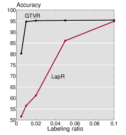
Classification accuracies of GTVR and LapR were then averaged over 30 tests for each labeling ratio and are shown in Figure 1. We see that GTVR achieves significantly higher accuracy than LapR for low labeling ratios. The failure of LapR at low labeling ratios is because an undirected graph fails to reveal the true structure.

Figure 1 also shows that the performance of GTVR saturates at around $95\%$. Many of the remaining errors are misclassification of blogs with many connections to the blogs from a different class, which violates the smoothness assumption underlying GTVR. Because of the same reason, the performance of a data-adaptive graph filter also saturates at around $95\%$ [22]. To improve on this performance may require using a more sophisticated classifier that we will pursue in future work.

Figure 1: Accuracy comparison of online blog classification as a function of labeling ratio.

VII-2 Bridge condition identification

We consider a semi-supervised regression problem, that is, regression with few labeled data and a large amount of unlabeled data [54]. The task is to predict the mass levels of unlabeled acceleration signals. We adopt the dataset of acceleration signals as described in Section VII-2. We randomly assigned known masses to 0.5%, 1%, 2%, 5%, and 10% of acceleration signals and applied the graph signal inpainting algorithms to estimate the masses for remaining nodes.

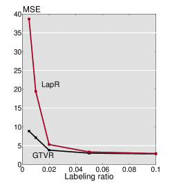
Figure 2 shows MSEs for estimated masses averaged over 30 tests for each labeling ratio. The proposed GTVR approach yields significantly smaller errors than LapR for low labeling ratios. Similarly to the conclusion of online blog classification, a direct graph adopted in GTVR reveals a better structure.

We observe that the performance of GTVR saturates at 3 in terms of MSE. This may be the result of how we obtain the graph. Here we construct the graph by using features from principal component analysis of the data. Since the data is collected with a real lab-scale model, which is complex and noisy, the principal component analysis may not extract all the useful information from the data, limiting the performance of the proposed method even with larger number of samples.

Figure 2: MSE comparison for the bridge condition identification as a function of labeling ratio.

Applications of graph signal matrix completion. We now apply the proposed algorithm to temperature estimation, recommender systems and expert opinion combination of online blog classification. We compare the proposed GMCR (30) with matrix completion algorithms. Those algorithms include SoftImpute [60], OptSpace [41], singular value thresholding (SVT) [61], weighted non-negative matrix factorization (NMF) [62], and graph-based weighted nonnegative matrix factorization (GWNMF) [63]. Similarly to the matrix completion algorithm described in Section 1, SoftImpute, OptSpace, and SVT minimize the rank of a matrix in similar, but different ways. NMF is based on matrix factorization, assuming that a matrix can be factorized into two nonnegative, low-dimensional matrices; GWNMF extends NMF by further constructing graphs on columns or rows to represent the internal information. In contrast to the proposed graph-based methods, GWNMF considers the graph structure in the hidden layer. For a fair comparison, we use the same graph structure for GWNMF and GMCM. NMF and GWNMF solve non-convex problems and get local minimum.

VII-1 Temperature estimation

We consider matrix completion, that is, estimation of the missing entries in a data matrix [35]. The task is to predict missing temperature values in an incomplete temperature data matrix where each column corresponds to the temperature values of all the weather stations from each day. We adopt the dataset of temperature data described in Section VII-3 [3]. In each day of temperature recording, we randomly hide $50\%,60\%,70\%,80\%,90\%$ measurements and apply the proposed matrix completion methods to estimate the missing measurements. To further test the recovery algorithms with different amount of data, we randomly pick 50 out of 365 days of recording and conduct the same experiment for 10 times. In this case, we have a graph signal matrix with $N=150$, and $L=50$, or $L=365$.

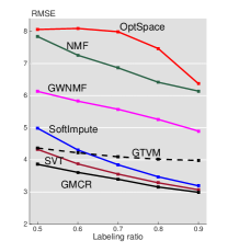
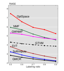
Figures 3 and 4 show RMSEs and MAEs for estimated temperature values averaged over 10 tests for each labeling ratio. We see that GTVM, as a pure graph-based method (26), performs well when the labeling ratio is low. When the labeling ratio increases, the performance of GTVM does not improve as much as the matrix completion algorithms, because it cannot learn from the graph signals. For both evaluation scores, RMSE and MAE, GMCR outperforms all matrix completion algorithms because it combines the prior information on graph structure with the low-rank assumption to perform a twofold learning scheme.

(a) 50 recordings.	(b) 365 recordings.

Figure 3: RMSE of temperature estimation for 50 recordings and 365 recordings.

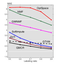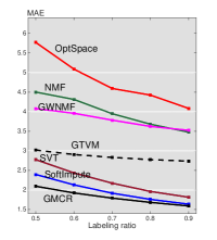(a) 50 recordings.	(b) 365 recordings.

Figure 4: MAE of temperature estimation for 50 recordings and 365 recordings.

VII-2 Rating completion for recommender system

We consider another matrix completion problem in the context of recommender systems based on the Jester dataset 1 [59]. The task is to predict missing ratings in an incomplete user-joke rating matrix where each column corresponds to the ratings of all the jokes from each user. Since the number of users is large compared to the number of jokes, following the protocol in [64], we randomly select 500 users for comparison purposes. For each user, we extract two ratings at random as test data for 10 tests. In this case, we have a graph signal matrix with $N=100$, and $L=500$.

Figures 5 and 6 show RMSEs and MAEs, defined in the evaluation score section, for estimated temperature values averaged over 10 tests. We see that graph-based methods (GWNMF and GMCR) take the advantage of exploiting the internal information of users and achieve smaller error. For RMSE, GMCR provides the best performance; for MAE, GWNMF provides the best performance.

Figure 5: RMSE of the rating completion in Jester 1 dataset.

Figure 6: MAE of the rating completion in Jester 1 dataset.

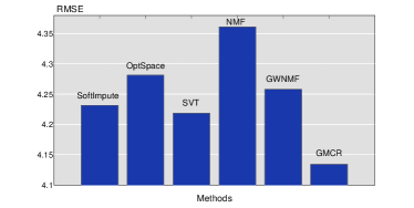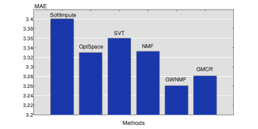VII-3 Combining expert opinions

In many real-world classification problems, the opinion of experts determines the ground truth. At times, these are hard to obtain; for instance, when a dataset is too large, obtaining the opinion of experts is too expensive, or experts differ among themselves, which happens, for example, in biomedical image classification [65]. In this case, a popular solution is to use multiple experts, or classifiers, to label dataset elements and then combine their opinions into the final estimate of the ground truth [66]. As we demonstrate here, opinion combining can be formulated and solved as graph signal matrix denoising.

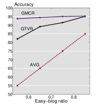
We consider the online blog classification problem. We hide the ground truth and simulate $K=100$ experts labeling $1224$ blogs. Each expert labels each blog as conservative ($+1$) or liberal ($-1$) to produce an opinion vector $\mathbf{t}_{k}\in\{+1,-1\}^{1224}$. Note that labeling mistakes are possible. We combine opinions from all the experts and form an opinion matrix $\operatorname{T}\in\{+1,-1\}^{1224\times 100}$, whose $k$th column is $\mathbf{t}_{k}$. We think of $\operatorname{T}$ as a graph signal matrix with noise that represents the experts’ errors. We assume some blogs are harder to classify than others (for instance, the content in a blog is ambiguous, which is hard to label), we split the dataset of all the blogs into “easy” and “hard” blogs and assume that there is a $90\%$ chance that an expert classifies an “easy” blog correctly and only a $30\%$ chance that an expert classifies a “hard” blog correctly. We consider four cases of “easy” blogs making up $55\%$, $65\%$, $75\%$, and $85\%$ of the entire dataset.

A baseline solution is to average (AVG) all the experts opinions into vector $\mathbf{t}_{\rm avg}=(\sum_{k}\mathbf{t}_{k})/K$ and then use the sign $\rm{sign}(\mathbf{t}_{\rm avg})$ vector as the labels to blogs. We compare the baseline solution with the GTVR solution (IV-1) and GMCR. In GTVR, we first denoise every signal $\mathbf{t}_{k}$ and then compute the average of denoised signals $\widetilde{\mathbf{t}}_{\rm avg}=(\sum_{k}\widetilde{\mathbf{t}}_{k})/K$ and use ${\rm sign}(\widetilde{\mathbf{t}}_{\rm avg})$ as labels to blogs.

Using the proposed methods, we obtain a denoised opinion matrix. We average the opinions from all the experts into a vector and use its signs as the labels to blogs. Note that, for GTVR and GMCR, the accessible part is all the indices in the opinion matrix $\operatorname{T}$; since each entry in $\operatorname{T}$ can be wrong, no ground-truth is available for cross-validation. We vary the tuning parameter and report the best results. Figure 7 shows the accuracy of estimating the ground-truth. We see that, through promoting the smoothness in each column, GTVR improves the accuracy; GMCR provides the best results because of its twofold learning scheme. Note that Figure 7 does not show that the common matrix completion algorithms provide the same “denoised” results as the baseline solution.

Figure 7: Accuracy of combining expert opinions.

Applications of robust graph signal inpainting. We now apply the proposed robust graph signal inpainting algorithm to online blog classification and bridge condition identification. In contrast to what is done in the applications of graph signal inpainting, we manually add some outliers to the accessible part and compare the algorithm to common graph signal inpainting algorithms.

VII-1 Online blog classification

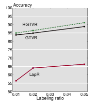
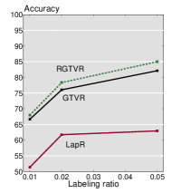
We consider semi-supervised online blog classification as described in Section VII-1. To validate the robustness of detecting outliers, we randomly mislabel a fraction of the labeled blogs, feed them into the classifiers together with correctly labeled signals, and compare the fault tolerances of the algorithms. Figure 8 shows the classification accuracies when $1\%,2\%$, and $5\%$ of blogs are labeled, with $16.66\%$ and $33.33\%$ of these labeled blogs mislabeled in each labeling ratio. We see that, in each case, RGTVR provides the most accurate classification.

(a) mislabeled ratio: 16.67%.	(b) mislabeled ratio: 33.33%.

Figure 8: Robustness to mislabeled blogs: accuracy comparison with labeling ratio of $1\%,2\%$ and $5\%$, and mislabeling ratio of $16.66\%$ and $33.33\%$ in each labeling ratio.

VII-2 Bridge condition identification

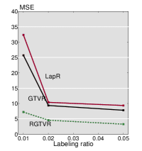
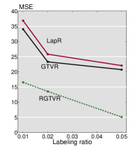
We consider a semi-supervised regression problem and adopt the dataset of acceleration signals as described in Section VII-2. To validate the robustness of facing outliers, we randomly mislabel a fraction of labeled acceleration signals, feed them into the graph signal inpainting algorithm together with correctly labeled acceleration signals, and compare the fault tolerances of the algorithms. Figure 9 shows MSEs when $1\%,2\%$, and $5\%$ of signals are labeled, with $16.66\%$ and $33.33\%$ of these labeled signals mislabeled in each labeling ratio. We see that, in each case, RGTVR provides the smallest error.

(a) 16.67%.	(b) 33.33%.

Figure 9: Robustness to mislabeled signals: MSE comparison with labeling ratio of $1\%,2\%$, and $5\%$, and mislabeling ratio of $16.66\%$ and $33.33\%$ in each labeling ratio.

VIII Conclusions

We formulated graph signal recovery as an optimization problem and provided a general solution by using the alternating direction method of multipliers. We showed that several existing recovery problems, including signal inpainting, matrix completion, and robust principal component analysis, are related to the proposed graph signal recovery problem. We further considered three subproblems, including graph signal inpainting, graph signal matrix completion, and anomaly detection of graph signals. For each subproblem, we provided specific solutions and theoretical analysis. Finally, we validated the proposed methods on real-world recovery problems, including online blog classification, bridge condition identification, temperature estimation, recommender system, and expert opinion combination of online blog classification.

IX Acknowledgment

We gratefully acknowledge support from the NSF through awards 1130616, 1421919, 1011903, 1018509, AFOSR grant FA95501210087, and the University Transportation Center grant-DTRT12-GUTC11 from the US Department of Transportation as well as the CMU Carnegie Institute of Technology Infrastructure Award. We also thank the editor and the reviewers for comments that led to improvements in the manuscript. We follow the principles of reproducible research. To that end, we created a reproducible research page available to readers [67]. Initial parts of this work were presented at ICASSP 2014 [47].

X Appendix

To decompose the graph total variation term and nuclear norm term, we introduce an auxiliary matrix $\operatorname{Z}$ to duplicate $\operatorname{X}$ and a residual matrix $\operatorname{C}$ to capture the error introduced by the inaccessible part of $\operatorname{T}$ in (6), and then rewrite (LABEL:eq:C_Opt) in the equivalent form

$$\widehat{\operatorname{X}},\widehat{\operatorname{W}},\widehat{\operatorname{E}},\widehat{\operatorname{Z}},\widehat{\operatorname{C}} = \arg\min_{\operatorname{X},\operatorname{W},\operatorname{E},\operatorname{Z},\operatorname{C}}\ \left\|\operatorname{W}\right\|_{F}^{2}+\alpha\operatorname{S}_{2}(\operatorname{Z})$$

$$+\beta\left\|\operatorname{X}\right\|_{*}+\gamma\left\|\operatorname{E}\right\|_{1}+\mathcal{I}(\operatorname{C}_{\mathcal{M}}),$$

subject to $$\operatorname{T}=\operatorname{X}+\operatorname{W}+\operatorname{E}+\operatorname{C}$$

$$\operatorname{Z}=\operatorname{X},$$

where $\mathcal{I}$ is an indicator operator defined as

$$\mathcal{I}(\operatorname{X})_{n,m}=\begin{cases}0,&\text{if \,\,\,}\operatorname{X}_{n,m}=0,\\ +\infty,&\text{otherwise}.\end{cases}$$

Note that we move $\left\|\operatorname{W}\right\|_{F}^{2}$ from the constraint to the objective function and putting $\mathcal{I}(\operatorname{C}_{\mathcal{M}})$ in the objective function is equivalent to setting $\operatorname{C}_{\mathcal{M}}$ to be zero. We then construct the augmented Lagrangian function

$$\mathcal{L}{(\operatorname{X},\operatorname{W},\operatorname{E},\operatorname{Z},\operatorname{C},\operatorname{Y}_{1},\operatorname{Y}_{2})}$$

$$= \left\|\operatorname{W}\right\|_{F}^{2}+\alpha\operatorname{S}_{2}{(\operatorname{Z})}+\beta\left\|\operatorname{X}\right\|_{*}+\gamma\left\|\operatorname{E}\right\|_{1}+\mathcal{I}{(\operatorname{C}_{\mathcal{M}})}$$

$$+<\operatorname{Y}_{1},\operatorname{T}-\operatorname{X}-\operatorname{W}-\operatorname{E}-\operatorname{C}>+<\operatorname{Y}_{2},\operatorname{X}-\operatorname{Z}>$$

$$+\frac{\eta}{2}\left\|\operatorname{T}-\operatorname{X}-\operatorname{W}-\operatorname{E}-\operatorname{C}\right\|_{F}^{2}+\frac{\eta}{2}\left\|\operatorname{X}-\operatorname{Z}\right\|_{F}^{2}.$$

We minimize for each variable individually. For $\operatorname{X}$, we aim to solve

$$\min_{\operatorname{X}}\beta\left\|\operatorname{X}\right\|_{*}+\frac{\eta}{2}\left\|\operatorname{T}-\operatorname{X}-\operatorname{W}-\operatorname{E}-\operatorname{C}-\operatorname{Y}_{1}\right\|_{F}^{2}+\frac{\eta}{2}\left\|\operatorname{X}-\operatorname{Z}-\operatorname{Y}_{2}\right\|_{F}^{2}.$$

We solve it by the standard matrix-soft thresholding (15); for $\operatorname{W}$, we aim to solve

$$\min_{\operatorname{W}}\left\|\operatorname{W}\right\|_{F}^{2}+\frac{\eta}{2}\left\|\operatorname{T}-\operatorname{X}-\operatorname{W}-\operatorname{E}-\operatorname{C}-\operatorname{Y}_{1}\right\|_{F}^{2}.$$

We obtain the closed-form solution by setting the derivative to zero; for $\operatorname{E}$, we aim to solve

$$\min_{\operatorname{E}}\gamma\left\|\operatorname{E}\right\|_{1}+\frac{\eta}{2}\left\|\operatorname{T}-\operatorname{X}-\operatorname{W}-\operatorname{E}-\operatorname{C}-\operatorname{Y}_{1}\right\|_{F}^{2}.$$

We solve it by standard soft thresholding (14); for $\operatorname{Z}$, we aim to solve

$$\min_{\operatorname{X}}\alpha\left\|\operatorname{Z}-\operatorname{A}\operatorname{Z}\right\|_{F}^{2}+\frac{\eta}{2}\left\|\operatorname{X}-\operatorname{Z}-\operatorname{Y}_{2}\right\|_{F}^{2}.$$

We obtain the closed-form solution by setting the derivative to zero. For $\operatorname{C}$, we just set $\operatorname{C}_{M}=0$ to satisfy the constraints; for $\operatorname{Y}_{1}$ and $\operatorname{Y}_{2}$, we update them as the standard Lagrange multipliers. For the final implementation see Algorithm 1.

References

- [1] M. Jackson, Social and Economic Networks. Princeton University Press, 2008.
- [2] M. Newman, Networks: An Introduction. Oxford University Press, 2010.
- [3] A. Sandryhaila and J. M. F. Moura, “Discrete signal processing on graphs,” IEEE Trans. Signal Process., vol. 61, no. 7, pp. 1644–1656, Apr. 2013.
- [4] ——, “Discrete signal processing on graphs: Frequency analysis,” IEEE Trans. Signal Process., vol. 62, no. 12, pp. 3042–3054, Jun. 2014.
- [5] D. I. Shuman, S. K. Narang, P. Frossard, A. Ortega, and P. Vandergheynst, “The emerging field of signal processing on graphs: Extending high-dimensional data analysis to networks and other irregular domains,” IEEE Signal Process. Mag., vol. 30, pp. 83–98, May 2013.
- [6] D. K. Hammond, P. Vandergheynst, and R. Gribonval, “Wavelets on graphs via spectral graph theory,” Appl. Comput. Harmon. Anal., vol. 30, pp. 129–150, Mar. 2011.
- [7] S. K. Narang and A. Ortega, “Perfect reconstruction two-channel wavelet filter banks for graph structured data,” IEEE Trans. Signal Process., vol. 60, no. 6, pp. 2786–2799, Jun. 2012.
- [8] ——, “Compact support biorthogonal wavelet filterbanks for arbitrary undirected graphs,” IEEE Trans. Signal Process., vol. 61, no. 19, pp. 4673–4685, Oct. 2013.
- [9] S. K. Narang, G. Shen, and A. Ortega, “Unidirectional graph-based wavelet transforms for efficient data gathering in sensor networks,” in Proc. IEEE Int. Conf. Acoust., Speech Signal Process., Dallas, TX, Mar. 2010, pp. 2902–2905.
- [10] I. Z. Pesenson, “Sampling in Paley-Wiener spaces on combinatorial graphs,” Trans. Amer. Math. Soc., vol. 360, no. 10, pp. 5603–5627, May 2008.
- [11] S. K. Narang, A. Gadde, and A. Ortega, “Signal processing techniques for interpolation in graph structured data,” in Proc. IEEE Int. Conf. Acoust., Speech Signal Process., Vancouver, May 2013, pp. 5445–5449.
- [12] X. Wang, P. Liu, and Y. Gu, “Local-set-based graph signal reconstruction,” IEEE Trans. Signal Process., 2014, submitted.
- [13] A. Agaskar and Y. M. Lu, “A spectral graph uncertainty principle,” IEEE Trans. Inf. Theory, vol. 59, no. 7, pp. 4338 – 4356, Jul. 2013.
- [14] S. Chen, F. Cerda, P. Rizzo, J. Bielak, J. H. Garrett, and J. Kovačević, “Semi-supervised multiresolution classification using adaptive graph filtering with application to indirect bridge structural health monitoring,” IEEE Trans. Signal Process., vol. 62, no. 11, pp. 2879 – 2893, Jun. 2014.
- [15] A. Sandryhaila and J. M. F. Moura, “Classification via regularization on graphs,” in IEEE GlobalSIP, Austin, TX, Dec. 2013, pp. 495–498.
- [16] V. N. Ekambaram, B. A. G. Fanti, and K. Ramchandran, “Wavelet-regularized graph semi-supervised learning,” in IEEE GlobalSIP, Austin, TX, Dec. 2013, pp. 423 – 426.
- [17] X. Zhang, X. Dong, and P. Frossard, “Learning of structured graph dictionaries,” in Proc. IEEE Int. Conf. Acoust., Speech Signal Process., Kyoto, Japan, 2012, pp. 3373–3376.
- [18] D. Thanou, D. I. Shuman, and P. Frossard, “Parametric dictionary learning for graph signals,” in IEEE GlobalSIP, Austin, TX, Dec. 2013, pp. 487–490.
- [19] P.-Y. Chen and A. Hero, “Local Fiedler vector centrality for detection of deep and overlapping communities in networks,” in Proc. IEEE Int. Conf. Acoust., Speech Signal Process., Florence, Italy, 2014, pp. 1120 – 1124.
- [20] A. Sandryhaila and J. M. F. Moura, “Big data processing with signal processing on graphs,” IEEE Signal Process. Mag., vol. 31, no. 5, pp. 80 – 90, 2014.
- [21] A. Elmoataz, O. Lezoray, and S. Bougleux, “Nonlocal discrete regularization on weighted graphs: A framework for image and manifold processing,” IEEE Trans. Image Process., vol. 17, no. 7, pp. 1047–1060, Jul. 2008.
- [22] S. Chen, A. Sandryhaila, J. M. F. Moura, and J. Kovačević, “Adaptive graph filtering: Multiresolution classification on graphs,” in IEEE GlobalSIP, Austin, TX, Dec. 2013, pp. 427 – 430.
- [23] X. Dong, P. Frossard, P. Vandergheynst, and N. Nefedov, “Clustering on multi-layer graphs via subspace analysis on Grassmann manifolds,” IEEE Trans. Signal Process., vol. 62, no. 4, pp. 905–918, Feb. 2014.
- [24] F. R. K. Chung, Spectral Graph Theory (CBMS Regional Conference Series in Mathematics, No. 92). Am. Math. Soc., 1996.
- [25] M. Belkin and P. Niyogi, “Laplacian eigenmaps for dimensionality reduction and data representation,” Neur. Comput., vol. 13, pp. 1373–1396, 2003.
- [26] M. Püschel and J. M. F. Moura, “Algebraic signal processing theory: Foundation and 1-D time,” IEEE Trans. Signal Process., vol. 56, no. 8, pp. 3572–3585, Aug. 2008.
- [27] ——, “Algebraic signal processing theory: 1-D space,” IEEE Trans. Signal Process., vol. 56, no. 8, pp. 3586–3599, Aug. 2008.
- [28] S. Mallat, A Wavelet Tour of Signal Processing, 3rd ed. New York, NY: Academic Press, 2009.
- [29] A. Buades, B. Coll, and J. M. Morel, “A review of image denoising algorithms, with a new one,” Multiscale Modeling & Simulation, vol. 4, pp. 490–530, Jul. 2005.
- [30] L. I. Rudin, Osher, and E. Fatemi, “Nonlinear total variation based noise removal algorithms,” Physica D, vol. 60, no. 1–4, pp. 259–268, Nov. 1992.
- [31] T. F. Chan, S. Osher, and J. Shen, “The digital TV filter and nonlinear denoising,” IEEE Trans. Image Process., vol. 10, no. 2, pp. 231–241, Feb. 2001.
- [32] A. Chambolle, “An algorithm for total variation minimization and applications,” J. Math. Imag. Vis., vol. 20, no. 1-2, pp. 89–97, Jan. 2004.
- [33] D. L. Donoho, “Compressed sensing,” IEEE Trans. Inf. Theory, vol. 52, no. 4, pp. 1289–1306, Apr. 2006.
- [34] E. J. Candés, J. K. Romberg, and T. Tao, “Stable signal recovery from incomplete and inaccurate measurements,” Comm. Pure Appl. Math., vol. 59, pp. 1207–1223, Aug. 2006.
- [35] E. J. Candés and B. Recht, “Exact matrix completion via convex optimization,” Journal Foundations of Computational Mathematics., vol. 9, no. 2, pp. 717–772, Dec. 2009.
- [36] E. J. Candés and Y. Plan, “Matrix completion with noise,” Proceedings of the IEEE, vol. 98, pp. 925–936, Jun. 2010.
- [37] E. J. Candés, X. Li, Y. Ma, and J. Wright, “Robust principal component analysis?” Journal of the ACM, vol. 58, May 2011.
- [38] J. Wright, A. Ganesh., S. Rao, Y. Peng, and Y. Ma, “Robust principal component analysis: Exact recovery of corrupted low-rank matrices by convex optimization,” in Proc. Neural Information Process. Syst., Dec. 2009, pp. 2080–2088.
- [39] T. F. Chan and J. Shen, “Variational image inpainting,” Comm. Pure Applied Math, vol. 58, pp. 579–619, Feb. 2005.
- [40] J. Mairal, M. Elad, and G. Sapiro, “Sparse representation for color image restoration,” IEEE Trans. Image Process., vol. 17, pp. 53–69, Jan. 2008.
- [41] R. H. Keshavan, A. Montanari, and S. Oh, “Matrix completion from noisy entries,” J. Machine Learn. Research, vol. 11, pp. 2057–2078, Jul. 2010.
- [42] M. Mardani, G. Mateos, and G. B. Giannakis, “Decentralized sparsity-regularized rank minimization: Algorithms and applications,” IEEE Trans. Signal Process., vol. 61, pp. 5374 – 5388, Nov. 2013.
- [43] A. Anis, A. Gadde, and A. Ortega, “Towards a sampling theorem for signals on arbitrary graphs,” in Proc. IEEE Int. Conf. Acoust., Speech Signal Process., May 2014, pp. 3864–3868.
- [44] X. Zhu, Z. Ghahramani, and J. Lafferty, “Semi-supervised learning using Gaussian fields and harmonic functions,” in Proc. ICML, 2003, pp. 912–919.
- [45] D. Zhou and B. Scholkopf, “A regularization framework for learning from graph data,” in ICML Workshop Stat. Rel. Learn., 2004, pp. 132–137.
- [46] M. Belkin, P. Niyogi, and P. Sindhwani, “Manifold regularization: A geometric framework for learning from labeled and unlabeled examples.” J. Machine Learn. Research, vol. 7, pp. 2399–2434, 2006.
- [47] S. Chen, A. Sandryhaila, G. Lederman, Z. Wang, J. M. F. Moura, P. Rizzo, J. Bielak, J. H. Garrett, and J. Kovačević, “Signal inpainting on graphs via total variation minimization,” in Proc. IEEE Int. Conf. Acoust., Speech Signal Process., Florence, Italy, May 2014, pp. 8267 – 8271.
- [48] S. Chen, A. Sandryhaila, J. M. F. Moura, and J. Kovačević, “Signal denoising on graphs via graph filtering,” in Proc. IEEE Glob. Conf. Signal Information Process., Atlanta, GA, Dec. 2014.
- [49] M. Vetterli, J. Kovačević, and V. K. Goyal, Foundations of Signal Processing. Cambridge University Press, 2014, http://www.fourierandwavelets.org/. [Online]. Available: http://www.fourierandwavelets.org/
- [50] D. Donoho and M. Elad, “Optimally sparse representation in general (nonorthogonal) dictionaries via minimization,” Proc. Nat. Acad. Sci., vol. 100, no. 5, pp. 2197–2202, Mar. 2003.
- [51] E. J. Candès and Y. Plan, “Near-ideal model selection by minimization,” Ann. Statist., vol. 37, no. 5A, pp. 2145–2177, 2009.
- [52] S. Boyd, N. Parikh, E. Chu, B. Peleato, and J. Eckstein, “Distributed optimization and statistical learning via the alternating direction method of multipliers,” Found. Trends Mach. Learn., vol. 3, no. 1, pp. 1–122, Jan. 2011.
- [53] S. Boyd and L. Vandenberghe, Convex Optimization. New York, NY, USA: Cambridge University Press, 2004, vol. 17, no. 7.
- [54] X. Zhu, “Semi-supervised learning literature survey,” Univ. Wisconsin-Madison, Tech. Rep. 1530, 2005.
- [55] L. A. Adamic and N. Glance, “The political blogosphere and the 2004 U.S. election: Divided they blog,” in Proc. LinkKDD, 2005, pp. 36–43.
- [56] F. Cerda, J. Garrett, J. Bielak, P. Rizzo, J. A. Barrera, Z. Zhang, S. Chen, M. T. McCann, and J. Kovačević, “Indirect structural health monitoring in bridges: scale experiments,” in Proc. Int. Conf. Bridge Maint., Safety Manag., Lago di Como, Jul. 2012, pp. 346–353.
- [57] F. Cerda, S. Chen, J. Bielak, J. H. Garrett, P. Rizzo, and J. Kovačević, “Indirect structural health monitoring of a simplified laboratory-scale bridge model,” Int. J. Smart Struct. Syst., Sp. Iss. Challenge on bridge health monitoring utilizing vehicle-induced vibrations, vol. 13, no. 5, May 2013.
- [58] G. Lederman, Z. Wang, J. Bielak, H. Noh, J. H. Garrett, S. Chen, J. Kovačević, F. Cerda, and P. Rizzo, “Damage quantification and localization algorithms for indirect SHM of bridges,” in Proc. Int. Conf. Bridge Maint., Safety Manag., Shanghai, Jul. 2014, pp. 640 – 647.
- [59] J. jokes. Http://eigentaste.berkeley.edu/user/index.php. [Online]. Available: http://eigentaste.berkeley.edu/user/index.php
- [60] R. Mazumder, T. Hastie, and R. Tibshirani, “Spectral regularization algorithms for learning large incomplete matrices,” J. Mach. Learn. Res., vol. 11, pp. 2287–2322, Aug. 2010.
- [61] J.-F. Cai, E. J. Candès, and Z. Shen, “A singular value thresholding algorithm for matrix completion,” SIAM J. on Optimization, vol. 20, no. 4, pp. 1956–1982, Mar. 2010.
- [62] S. Zhang, W. Wang, J. Ford, and F. Makedon, “Learning from incomplete ratings using non-negative matrix factorization,” in In Proc. of SIAM Conference on Data Mining (SDM), 2006, pp. 549–553.
- [63] Q. Gu, J. Zhou, and C. Ding, “Collaborative filtering: Weighted nonnegative matrix factorization incorporating user and item graphs,” in In Proc. of SIAM Conference on Data Mining (SDM), 2010, pp. 199–210.
- [64] R. H. Keshavan, A. Montanari, and S. Oh, “Low-rank matrix completion with noisy observations: A quantitative comparison,” in Proceedings of the 47th Annual Allerton Conference on Communication, Control, and Computing, ser. Allerton’09, 2009, pp. 1216–1222.
- [65] A. Kuruvilla, N. Shaikh, A. Hoberman, and J. Kovačević, “Automated diagnosis of otitis media: A vocabulary and grammar,” Int. J. Biomed. Imag., Sp. Iss. Computer Vis. Image Process. for Computer-Aided Diagnosis, Aug. 2013.
- [66] S. R. Cholleti, S. A. Goldman, A. Blum, D. G. Politte, S. Don, K. Smith, and F. Prior, “Veritas: Combining expert opinions without labeled data.” International Journal on Artificial Intelligence Tools, vol. 18, no. 5, pp. 633–651, 2009.
- [67] S. Chen, A. Sandryhaila, J. M. F. Moura, and J. Kovačević. (2015) Signal recovery on graphs: Variation minimization. Http://jelena.ece.cmu.edu/repository/rr/15_ChenSMK/15_ChenSMK.html.