Two-Dimensional Clusters of Colloidal Spheres: Ground States, Excited States, and Structural Rearrangements

Abstract

We study experimentally what is arguably the simplest yet non-trivial colloidal system: two-dimensional clusters of 6 spherical particles bound by depletion interactions. These clusters have multiple, degenerate ground states whose equilibrium distribution is determined by entropic factors, principally the symmetry. We observe the equilibrium rearrangements between ground states as well as all of the low-lying excited states. In contrast to the ground states, the excited states have soft modes and low symmetry, and their occupation probabilities depend on the size of the configuration space reached through internal degrees of freedom, as well as a single “sticky parameter” encapsulating the depth and curvature of the potential. Using a geometrical model that accounts for the entropy of the soft modes and the diffusion rates along them, we accurately reproduce the measured rearrangement rates. The success of this model, which requires no fitting parameters or measurements of the potential, shows that the free-energy landscape of colloidal systems and the dynamics it governs can be understood geometrically.

Colloidal clusters containing a few particles bound together by weak attractive interactions are among the simplest, non-trivial systems for investigating collective phenomena in condensed matter. Such clusters can equilibrate on experimental time scales and display complex dynamics, yet are small enough that the ground states can be enumerated theoretically, and the positions and motions of all the particles can be measured experimentally. Theoretical and experimental work on isolated three-dimensional (3D) colloidal clusters of monodisperse particles has shown how the number of ground states changes with the number of particles $N$ arkus09; arkus_deriving_2011; hoy_minimal_2010; hoy12; holmes14; hoy15 and how the free energies of the rigid states are related to entropy-reducing symmetry effects and entropy-enhancing vibrational modes meng10; wales10; calvo12. The importance of entropy in colloidal clusters stands in stark contrast to the case of atomic clusters, where potential energy effects dominate. The entropically-favored clusters are important clues to understanding nucleation barriers in bulk colloidal fluids crocker10; hoy12 and the local structure of gels royall_direct_2008.

However, the excited states and structural rearrangements in such clusters have not yet been studied experimentally. In bulk materials, local structural rearrangements are important to a variety of dynamical phenomena, including the glass transition weeks_properties_2002, aging brito_heterogeneous_2007; yunker_irreversible_2009, epitaxial growth ganapathy10, and the jamming transition lois_jamming_2008. A better understanding of the internal dynamics in colloidal clusters could reveal local mechanisms underpinning these bulk phenomena. Only a few experimental studies have explored internal dynamics in colloidal clusters: Perry and coworkers examined transitions between two states of a 3D 6-particle cluster of spherical particles perry12; Yunker and coworkers studied relations between the vibrational mode structure and the contact network in disordered, two-dimensional (2D) clusters of polydisperse particles as a function of $N$ yunker11; yunker_relationship_2013; and Chen and coworkers examined the interconversion and aggregation pathways in clusters of particles with directional attractions chen11a. As yet, however, a quantitative understanding of the rearrangement rates and the pathways through the excited states remains challenging. Transition-state models eyring35; wigner38; horiuti38; morgan14, which relate dynamics to the heights of saddle points on the energy landscape, are not easily applied to colloids because the fluid surrounding the particles damps and hydrodynamically couples their motions, and the short-ranged interactions typical of colloidal particles are not easily measured, making the topography of the landscape difficult to accurately compute. Indeed, as we shall show, the excited state occupation probabilities and the transition rates are sensitive to fine details of the potential, which are not easily measured.

Figure 1: (a) SDS micelles induce a short-range depletion attraction between polystyrene microspheres and between the microspheres and the nearby glass coverslip. (b) Time-lapse images demonstrate a transition. (c) The three rigid ground states and their theoretical and experimental probabilities with 95% confidence intervals Note1 (the probabilities for the parallelogram include both chiral enantiomers).

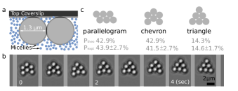
We study experimentally the excited states and rearrangement rates in perhaps the simplest type of colloidal cluster: isostatic arrangements of equal-sized, spherical colloidal particles, constrained to lie on a plane and held together by well-controlled, short-range attractions a few times the thermal energy $k_{B}T$ in depth (Figure 1a). Because the clusters are isostatic, all excited states have zero-frequency modes, or soft modes, in their vibrational spectra (Figure 1b, Note1). By tracking the particles over long times, we quantify the equilibrium probability of each excited state and the motions of the particles within each soft mode. Surprisingly, the dynamics that emerge from this landscape can be quantitatively described by a simple geometric model involving only two parameters, a “sticky parameter” that characterizes both the depth and curvature of the attraction, and a diffusion coefficient, which we find to be insensitive to the mode. Both parameters can be easily measured. Therefore, no detailed knowledge of the interactions or hydrodynamics is required to reproduce the rates of rearrangement between ground states.

To make clusters, we first load an aqueous suspension of 1.3 $\mu$m-diameter sulfate polystyrene microspheres into a cell made from two plasma-cleaned glass coverslips separated by 35 $\mu$m DuPont Mylar^® A spacers Note1. The only additional component in the suspension is sodium dodecyl sulfate (SDS), a surfactant that forms negatively charged micelles in solution. The micelles create a weak depletion interaction asakura54; vrij76; iracki10 between the particles and a stronger depletion interaction between the particles and coverslip lekkerkerker11; kaplan94b, as illustrated in Figure 1a. At 33.4 mM SDS, we observe that 2D clusters bound to a coverslip frequently transition between states but rarely split apart or merge Note1. At this concentration, the sodium counterions from the surfactant reduce the Debye length to 2.85 nm, setting the effective hard-sphere depletion range of the micelles to 30 nm, just 2.3% of the particle diameter tulpar01; iracki10. As a result, the electrostatic and depletion interactions between the particles are short-ranged. There is likely also a short-range van der Waals attraction, which we estimate tapers off to $k_{B}T$ when the particle surfaces are 145 nm apart israelachvili2011.

At the beginning of the experiment, we assemble clusters at the top of the sample cell using optical tweezers. We then turn off the tweezers and record digital micrographs for the remainder of the experiment. The clusters, which would normally sediment, remain at the underside of the upper coverslip, confirming the depletion attraction. We use particle tracking algorithms to locate the particles crocker96, link the locations into trajectories through time, and automatically identify the cluster configurations Note1.

We focus on 6-particle clusters because this is the smallest system with multiple ground states. Because these clusters are bound by short-range interactions, the potential energy is proportional to the number of contacts or “bonds” between particles. The 6-particle clusters adopt three ground states with nine bonds each (Figure 1c): the parallelogram (which has two enantiomers), chevron, and triangle. In aggregate, the clusters occupy the parallelogram and chevron states for equal amounts of time but spend only one third as much time in the triangle state (Figure 1c). The measured occupation probabilities agree with the expectation for a statistical mechanics ensemble in equilibrium. To calculate the probabilities, we assume that the translational, rotational, and vibrational degrees of freedom are independent, the vibrational modes are harmonic, and the translational contributions and potential energy differ negligibly among the 3 states Note1. As seen previously in 3D clusters, the differences in occupation probabilities are primarily due to symmetry, which enters into the rotational contribution meng10; crocker10.

Figure 2: Theoretical (bars) and experimental (points) probability distributions of the 8 and 7-bond excited states. Each bar-point pair is labeled by a connectivity diagram of the excited state, with hinge-like joints and non-rigid squares labeled in red. Hand symbols mark the chiral states, and curved arrows mark the states with 2-fold rotational symmetry (in 2D the only accessible symmetry axis is perpendicular to the plane of confinement). The total observation time is 25.6 hours; for comparison, the clusters spend 19.5 hours in the 9-bond states. Error bars represent 95% confidence intervals Note1.

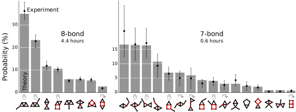
The excited states of the system have more complex and interesting structures. All of them have zero-frequency modes. The modes we see at the 8-bond energy level have either hinge-like joints or diamond-square-diamond lipscomb66 flexibility (Figure 2). Although the 7-bond energy level has twice as many states, nearly all of the zero-frequency modes are simply combinations of these two types of motion (Figure 2). The exceptions are a state with a flexible ring of five spheres and a state with a single sphere detached from the cluster. We do not include this disconnected state in our 7-bond probability calculations because it is not a true 6-sphere cluster.

The fraction of time the clusters spend in the excited energy levels depends on the surfactant concentration. At a concentration of 33.4 mM SDS, the clusters spend 95.5% of the time in states with 7 or more bonds. Of this time, 79.6% is spent in ground states, 18.0% in 8-bond excited states, and 2.4% in 7-bond excited states. As we decrease the surfactant concentration, the distribution shifts toward the excited energy levels. Qualitatively, this shift makes sense, since decreasing surfactant concentration corresponds to decreasing depletion strength. To understand the energy level occupation probabilities quantitatively, we must consider the entropy of the soft modes. We return to this point later.

Despite the wide variety of structures in the excited states, few have any symmetry. Surprisingly, the few symmetric states do not occur as infrequently as we might expect, given the dominant role symmetry—more specifically, permutational entropy meng10; gilson_symmetry_2010—plays in the probabilities of 6-sphere ground states in both 2D and 3D. Furthermore, the asymmetric states have a highly non-uniform distribution that is only partially explained by the increased probability of states that are pairs of chiral enantiomers (Figure 2). These observations suggest that the variation in probabilities arises from entropic factors other than the permutational contribution.

Table 1: Structural rearrangement rates between each of the ground states: (P)arallelogram, (C)hevron, and (T)riangle. In total, we observed 820 transitions in 25.6 hours of data from 44 clusters. Measured values used in postfactor: $D=0.065$ $\mu$m²/s (234 $\mu$m²/hr), $\kappa=30.5$ and $d$ = 1.3 $\mu$m.

		Theory									Experiment
		(nondimensional)				(per hour)					(per hour)
		end state
start state		P	C	T		P	C	T			P	C	T
	P	1.17	1.43	0.67		5.3	6.5	3.0			4.4	5.5	2.5
	C	1.43	2.31	0.56	$\times\frac{D}{\kappa d^{2}}$=	6.5	10.5	2.5			5.4	7.7	1.9
	T	0.67	0.56	0		3.0	2.5	0.00			2.5	2.2	0.04

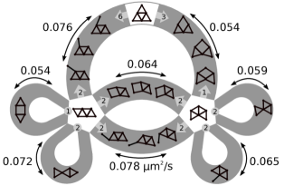
We also measure the rate of rearrangements between ground states and find that the matrix of rearrangements per unit time is symmetric (Table 1), as expected in equilibrium. Most of these rearrangements involve a single bond breaking, followed by the cluster diffusing along the soft mode in its excited state and finally forming a new bond to arrive at a ground state (Figure 3).

Understanding the excited state probabilities and rearrangement rates requires us to consider the entropy of the soft modes and the dynamics along the resulting free-energy landscape. In contrast to typical molecular-scale transitions, in which the potential energy varies along the entire reaction coordinate, our clusters first break out of a narrow attractive well and then freely diffuse in soft modes at constant potential energy under only an entropic driving force. We therefore expect the transition rates to depend on the entropy along the modes, the hydrodynamic drag, and the distance to diffuse in the soft modes.

To calculate the entropy, we use the geometrical model of reference holmes13. In this model, the potential energy landscape is represented as a collection of manifolds, each at constant potential energy. The dimension of each manifold equals the number of internal degrees of freedom of the cluster: for example, the ground states are 0-dimensional manifolds (points), and the 8-bond states live on 1-dimensional manifolds (lines). To compute the partition function, we numerically parametrize each manifold and integrate the vibrational and rotational entropies over its entire volume. This calculation of the entropy is purely geometrical and requires no knowledge of the actual pair potential; the only assumption is that the harmonic vibrational degrees of freedom equilibrate quickly compared to motion along the soft modes.

The model reproduces our experimental measurements of the excited state probabilities within experimental error (Figure 2). The agreement validates the model’s assumption and shows that for the excited states, the entropy associated with the soft modes dominates the permutational entropy associated with asymmetry. In particular, the entropy of the zero-frequency modes explains the surprisingly high probability of 7-bond structures with 2-fold symmetry.

To understand the relative populations of the excited-state energy levels (8-bond versus 7-bond), we must consider the interparticle potential. Measuring the potential well is difficult because the interaction is short-ranged—only a few tens of nanometers for the depletion component iracki10 and similarly ranged for the electrostatic and van der Waals contributions. However, the short range makes it possible to use a “sticky sphere” approximation, in which a single parameter $\kappa$, called the “sticky parameter,” characterizes the interaction. $\kappa$ is the partition function for a single bond and as such is proportional to the amount of time two particles are bound versus separated. In the limit where the potential becomes both infinitely narrow and infinitely deep holmes13,

$$\kappa=\frac{e^{-\beta U_{0}}}{d\sqrt{\frac{2}{\pi}\beta U^{\prime\prime}_{0}}}$$ (1)

where $\beta=\frac{1}{k_{B}T}$, $U_{0}$ is the depth of the potential well, $d$ is the microsphere diameter, and $U^{\prime\prime}_{0}$ is the curvature at the potential minimum. The advantage of this approximation is that we need only measure $\kappa$, and not the full potential.

We measure $\kappa$ from ratios of occupation probabilities of ground and excited energy levels. The total time $t_{n}$ for which a cluster has $n$ bonds is proportional to $Z_{n}\kappa^{n}$, where $Z_{n}$ is the sum of the partition functions of the $n$-bond manifolds Note1. By taking ratios of the time spent at different energy levels and calculating the $Z_{n}$ we obtain a measurement of the sticky parameter as $\kappa=\frac{t_{n+1}}{t_{n}}\frac{Z_{n}}{Z_{n+1}}$. We use observations of smaller clusters to determine $\kappa$ independently of our 6-particle data. For 3-particle clusters, with 3-bond and 2-bond energy levels, we find $\kappa$ = 29.3. We make two more measurements of $\kappa$ using 4-particle clusters: a comparison of 5-bond to 4-bond energy levels yields $\kappa$ = 26.8, and that of 4-bond to 3-bond levels yields $\kappa$ = 35.3. Using the mean of these measurements (30.5) in the $n$-bond partition function $Z_{n}\kappa^{n}$, normalized by $\sum_{n=7}^{9}Z_{n}\kappa^{n}$ where $[Z_{7},Z_{8},Z_{9}]=[11900,3320,498]$, we predict 6-particle occupation probabilities of $p_{7}=2.1\pm 0.6\%$, $p_{8}=17.6\pm 2.0\%$, and $p_{9}=80.3\pm 2.5\%$, where the uncertainties are based on the range of measured $\kappa$ values. The calculations agree with our measured occupation probabilities.

Figure 3: The 8-bond excited states form transition pathways (gray background) between the ground states (white background). The numbers at the edges of the ground states show the number of bonds that lead into each nearby pathway. The measured diffusion coefficients of the modes range from 0.054 to 0.078 $\mu$m²/s Note1.

The transition rates are calculated using Transition Path Theory (TPT) weinan10; holmes13. To simplify the calculations we suppose that each transition occurs by a single bond breaking, followed by the cluster diffusing along a 1-dimensional path and forming another bond. We calculate the flux of probability along each path and from this extract the non-dimensional rates, exactly as in reference holmes13. The dimensional rates are obtained by multiplying by $D/\kappa d^{2}$, where $D$ is the average diffusion coefficient and $d$ is the microsphere diameter (Table 1). As our implementation of the model ignores the time the clusters spend with fewer than 8 bonds, we expect it to slightly overestimate the rates.

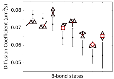
To determine the second parameter in our model, $D$, we measure the mean-square displacements along each pathway Note1. The measured diffusion coefficients range from 0.054 to 0.078 $\mu$m²/s with a mean of 0.065 $\mu$m²/s (Figure 3). The error bars on the measured diffusion coefficients Note1 are smaller than the variation in these values between the different modes. Thus the variation is likely due to differences in hydrodynamic friction factors between these modes, and not measurement error.

Nonetheless, the dimensional transition rates predicted from a simple model using a single, average diffusion coefficient agree with the measured rates, as shown in Table 1. Using different diffusion coefficients for each pathway yields values that agree equally well, though not better, with the data. This shows that the variation in diffusion coefficients among the different modes is not significant compared to the error in the measured transition rates. However, it also raises the question of why the diffusion coefficients for different pathways vary by only about 20% from the mean value. To understand this variation, we measure the diffusion coefficient for a rearrangement in a 3-sphere cluster and find a value of $D=$ 0.070 $\mu$m²/s, close to the average value for the 6-sphere rearrangement pathways. This agreement, along with the fact that these diffusion coefficients are all lower than that for a single sphere diffusing on the plane ($D=$ 0.10 $\mu$m²/s), suggests that the hydrodynamic friction factor along each pathway is dominated by flows between those spheres that must slide or roll past one another (as in the 3-sphere cluster), rather than by hydrodynamic interactions between larger moving subunits of the clusters. This would explain why the diffusion coefficients are similar for both diamond-square-diamond and hinge-like modes.

Taken together, these results shed new light on the free-energy landscape, and the dynamics along it, in colloidal systems. As in 3D clusters, the short-range interaction in our 2D system leads to degeneracy in both the ground and excited states. Whereas the occupation probabilities of the ground states are determined primarily by symmetry (permutational entropy), those of the excited states are determined primarily by the entropy of the soft modes. The agreement between the measured probabilities of the excited states and those predicted from our geometrical model shows that the harmonic vibrational modes equilibrate quickly compared to motion along the soft modes. This separation of timescales is another consequence of the short-range interactions. From our geometrical model of the free-energies, we can reproduce the measured rearrangement rates between ground states by incorporating only a single diffusion coefficient and the partition function of a single bond, both of which are easily measured.

Our model easily extends to 3D clusters. Its success in describing the 2D experimental data suggests that, at least near the isostatic limit, it may be possible to use similar geometrically-inspired models to understand the free-energy landscape and predict dynamics in more complex systems with soft modes, such as bulk colloidal phases. Indeed, such models are beginning to be developed jenkins2014.

* vnm@seas.harvard.edu

Supplemental Material

I I. Sample preparation protocol

1. Prepare one small (22x22 mm) and one large (24x60 mm) glass coverslip (VWR Micro Cover Glasses, No. 1) by rinsing with deionized water, drying with high-purity compressed nitrogen, and plasma cleaning for 10 minutes in a PDC-32G Plasma Cleaner/Sterilizer (Harrick Plasma) with the RF Level set to High.
   

2. To make a sample chamber, center the small coverslip on the large coverslip and separate them with narrow strips of 30 $\mu$m thick Mylar^® A film parallel to the long edges of the large coverslip. With the two coverslips clamped together (e.g., with binder clips), use UV-curing Norland Optical Adhesive 61 and a UV lamp to seal the two edges of the small coverslip parallel to the spacers. We find that sealing the four corners and then removing the clips and sealing along the two edges works well.
   

3. Use a pipette to dispense well-dispersed colloidal suspension near one of the unsealed edges of the small coverslip and let capillary action fill the sample chamber. We use a microsphere volume fraction of $7.6\times 10^{-6}$.
   

4. Use Devcon 5 Minute^® Epoxy to seal the last two edges of the small coverslip and to go over the two previously sealed edges for extra protection.
   

II II. Image acquisition, processing, and cluster configuration identification

To collect images, we use a Nikon Eclipse TI-E inverted microscope with a Photon Focus camera, a CameraLink cable, and an Epix frame grabber connected to a desktop PC. We use a combination of a 60$\times$ water immersion objective (Nikon CFI Plan Apo VC, NA 1.2) and a 1.5$\times$ tube lens. We choose a slow frame rate of 3 frames per second to efficiently capture many transitions while still collecting a few frames during each transition. This frame rate is high enough to allow particle tracking as described below.

By establishing four clusters of six particles in the field of view (59 $\mu$m $\times$ 59 $\mu$m), we can theoretically capture four hours of cluster data from a typical one hour experiment. In reality, 10 of our 44 clusters produced data for the entire duration of the data acquisition. The data series from the other 34 clusters were truncated during post-processing for one of four reasons: the cluster diffused to the edge of the frame (7 of 44); a particle permanently broke away from the cluster (7 of 44); the cluster came less than one particle diameter from merging with another cluster (7 of 44); or the particle locating or tracking algorithm failed because, for example, the optical system drifted out of focus (13 of 44). From 10.2 hours of raw video, we were able to obtain 25.6 hours of 6-particle cluster time series out of a theoretical maximum of 40.7 hours, a 63% recovery rate. While we do lose track of many of our clusters over time, this approach to data acquisition requires little supervision and produces twice as much usable data per hour as compared to watching over and tending to a single cluster.

Our post-processing routines are written in Python using the SciPy ecosystem jones01. We locate the particles, identify the clusters they belong to, and track the particles from frame to frame. To locate the particles, we first divide each image by a background image captured with no particles in the field of view to remove static artifacts. We then use the Crocker and Grier centroiding method crocker96 to locate the particles with better than 20 nm precision, as determined by tracking single particles diffusing in two dimensions at 500 frames per second, and then measuring the deviation from linearity of the mean-square displacements at the smallest lag times. After locating each of the particles, we identify the cluster that each particle belongs to by computing the distance to the four clusters’ centers in the preceding frame and selecting the cluster with the shortest distance. We then subtract off the cluster’s center of mass from each of the particle locations before linking them into trajectories solely using proximity between locations in consecutive images. Subtracting off the cluster center of mass reduces the apparent distance moved by the particles between frames by removing rigid-body translations. For our close-packed particles that occasionally diffuse distances greater than a full particle radius between frames, subtracting off the cluster center of mass prevents multiple particles from being linked to a single particle in the next frame. Alternative approaches to tracking a collection of close-packed particles include the optimization scheme of crocker96 and simply using strict proximity at a sufficiently high frame rate, where diffusing more than a particle radius between frames is extremely unlikely.

Figure 1: An adjacency matrix is a representation of the connectivity of a cluster. Each element in the matrix relates a pair of particles identified by the row number and column number; a value of 1 signifies bound, and 0 signifies unbound. The adjacency matrix of the pictured 8-bond excited state is shown as an example.

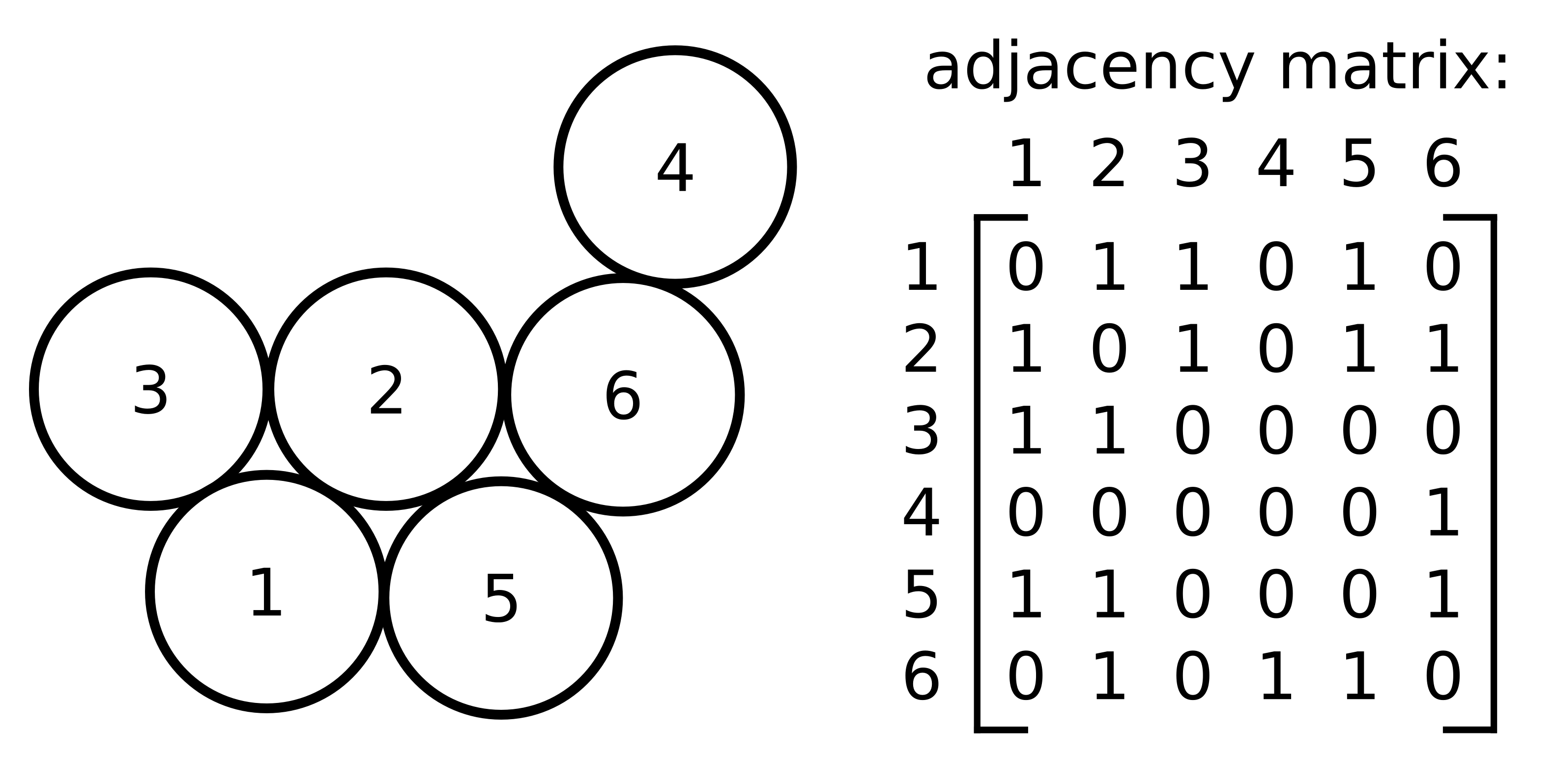
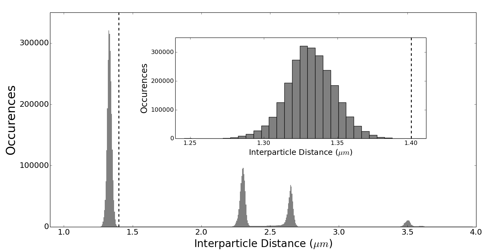
Once all the particles are found, assigned to clusters, and tracked, we determine the configuration of each cluster in each frame by computing the cluster’s adjacency matrix arkus_deriving_2011 (Figure 1). The adjacency matrix uniquely determines the cluster configuration, including the particular permutation of particles, from our library of configurations with 9-bonds, 8-bonds, 7-bonds, and “other” for clusters with fewer bonds. Such adjacency matrices do not distinguish between chiral enantiomers, which we pair together as single configurations. To determine when particles are bound or unbound, we set a cutoff distance of 1.4 $\mu$m, which is determined from the histogram in Figure 2. We find that the occupation probabilities are insensitive to the choice of cutoff distance.

Figure 2: Distances between all particles within all 6-particle clusters at all times. The first peak represents bound particles at distance $a\approx 1.33$ $\mu$m. The other peaks are at $\sqrt{3}a$, $2a$, and $\sqrt{7}a$ as expected for close-packed spheres on a plane. The width of the peaks comes from a combination of the particle polydispersity, the width of the interaction potential, and the precision of the particle locating algorithm.

III III. Ground state probability calculation

Each of the macroscopic ground states—the parallelogram, chevron, and triangle—consists of many microscopic states, so we need to consider entropy in addition to energy in our probability calculations meng10. The probability of a macroscopic ground state $s$ is given by the state’s classical configurational integral, $Z_{s}$, normalized by the sum over all the ground states:

$$P_{s}=\frac{Z_{s}}{\sum_{s^{\prime}}{Z_{s^{\prime}}}}.$$ (1)

Conveniently, $Z_{s}$ may be split into approximately independent translational, rotational, and vibrational components in addition to the contribution from the potential energy: $Z_{s}=Z_{t,s}Z_{r,s}Z_{v,s}e^{-\beta U_{s}}$. The translational component is identical for each ground state because the area of the glass coverslip the clusters can explore is about seven orders of magnitude larger than the area of a cluster. Additionally, each of the ground states has nine identical bonds, so the potential energy contribution is also identical for each ground state. By canceling out these contributions, we arrive at a probability expression that depends only on the rotational and vibrational components:

$$P_{s}=\frac{Z_{t,s}Z_{r,s}Z_{v,s}e^{-\beta U_{s}}}{\sum_{s^{\prime}}{Z_{t,s^{\prime}}Z_{r,s^{\prime}}Z_{v,s^{\prime}}e^{-\beta U_{s}^{\prime}}}}=\frac{Z_{t}e^{-\beta U}Z_{r,s}Z_{v,s}}{Z_{t}e^{-\beta U}\sum_{s^{\prime}}{Z_{r,s^{\prime}}Z_{v,s^{\prime}}}}=\frac{Z_{r,s}Z_{v,s}}{\sum_{s^{\prime}}{Z_{r,s^{\prime}}Z_{v,s^{\prime}}}}.$$ (2)

The following calculations are for identical microspheres, so we normalize the masses, interparticle distances, and spring constants to unity.

The rotational component of the classical configurational integral in systems of identical colloidal clusters depends on the state’s moment of inertia $I_{s}$, chirality $\chi_{s}$, and symmetry number $\sigma_{s}$, which accounts for the effects of permutations gilson_symmetry_2010:

$$Z_{r,s}\propto\frac{\chi_{s}\sqrt{I_{s}}}{\sigma_{s}}.$$ (3)

The moment of inertia is more generally the determinant of the moment of inertia tensor, but here the cluster has only one rotational axis. The chirality $\chi_{s}$ is 1 if the configuration is achiral and 2 if the configuration is a pair of chiral enantiomers.

To compute the vibrational contribution to the ground state probabilities, we use the harmonic approximation for the interparticle interactions. The vibrational contribution is inversely proportional to the product of the frequencies of the normal modes. There are $2N-3$ normal modes, since there are $2N$ degrees of freedom, and we have already removed 2 translational degrees of freedom and accounted for 1 rotational degree of freedom. The vibrational frequencies are given by the square root of the non-zero eigenvalues of the matrix $\boldsymbol{H_{s}}$, constructed from $N\times N$ super-elements. Each super-element is a $2\times 2$ Hessian matrix describing the interactions between particles $i$ and $j$ eyal06:

$$H_{ij}=\begin{bmatrix}\frac{\partial^{2}U}{\partial x_{i}\partial x_{j}}&\frac{\partial^{2}U}{\partial x_{i}\partial y_{j}}\\ \frac{\partial^{2}U}{\partial x_{j}\partial y_{i}}&\frac{\partial^{2}U}{\partial y_{i}\partial y_{j}}\end{bmatrix}.$$ (4)

The eigenvalues $k_{\alpha,s}$ of $\boldsymbol{H_{s}}$ are the squares of the normal mode frequencies, which allow us to compute the vibrational contribution to the classical configuration integral:

$$Z_{v,s}\propto\prod_{\alpha=1}^{2N-3}{\sqrt{\frac{1}{k_{\alpha,s}}}}.$$ (5)

This expression for the vibrational contribution is the last piece we need in order to use Equation 2 to calculate the probabilities of the parallelogram, chevron, and triangle. The results are presented in Table 1.

		Parallelogram	Chevron	Triangle
	$\sqrt{I_{s}}$	$\sqrt{5\frac{1}{2}}$	$\sqrt{4\frac{5}{6}}$	$\sqrt{5}$
	$\chi_{s}$	2	1	1
	$\sigma_{s}$	2	1	3
	$Z_{r,s}$	$\sqrt{5\frac{1}{2}}$	$\sqrt{4\frac{5}{6}}$	$\frac{1}{3}\sqrt{5}$
	$Z_{v,s}$	$\frac{8}{27}\sqrt{\frac{2}{11}}$	$\frac{8}{27}\sqrt{\frac{6}{29}}$	$\frac{8}{27}\sqrt{\frac{1}{5}}$
	Probability	$\frac{3}{7}$	$\frac{3}{7}$	$\frac{1}{7}$

Table 1: Comparison of the components factoring into the probabilities of the 3 ground states for two-dimensional clusters of 6 particles.

IV IV. Occupation probability error bars

The empirical occupation probability of each excited state is computed by taking the total amount of time we observe its adjacency matrix, and dividing by the total time spent in all configurations with identical energy. To estimate the error bar on this statistic we need to know the number of effectively independent samples. In general this is not the same as the number of data points, since the data are correlated in time: if a cluster has a particular adjacency matrix during one time step, it it more likely to remain in that adjacency matrix in subsequent time steps. After enough time steps, however, the data becomes decorrelated, and only then can new data be treated as independent. Roughly, the number of effectively independent samples is the length of the data, divided by the “correlation time” of the data.

A cluster can be thought of as a stochastic process $X_{t}\in\mathbb{R}^{2N}$, where $X_{t}$ lists the positions of the particles. An adjacency matrix corresponds to a subset $A\subset\mathbb{R}^{2N}$ of configuration space. We would like to know the average amount of time the system spends in set $A$, which we write as $p_{A}=\mathbb{E}1_{(X_{t}\in A)}$.

Let’s define a process $X_{A}(t)\equiv 1_{(X_{t}\in A)}$ to be the process that is 1 if $X(t)\in A$, and 0 otherwise. Then $p_{A}=\mathbb{E}X_{A}(t)$. Let $\hat{p}_{A}=\frac{1}{T}\int_{0}^{T}X_{A}(t)dt$ be an estimator for $p_{A}$. Let’s suppose this estimator is Gaussian, i.e. $\hat{p}_{A}=p_{A}+\sigma_{A}z_{A}$, where $\sigma_{A}$ is the standard deviation of the estimator, and $z_{A}\sim N(0,1)$ is a copy of the standard normal. Then, we can construct construct 95% error bars as $e=1.96\sigma_{A}$.

How can we determine the standard deviation $\sigma_{A}$? If each observation were independent, then we would have $\sigma_{A}^{2}=\frac{\sigma_{A,0}^{2}}{n},$ where $\sigma_{A,0}$ is the standard deviation of $X_{A}(t)$ at a single point in time (equal to $p_{A}(1-p_{A})$ for our process since it’s an indicator function), and $n$ is the number of independent observations.

For a process that is correlated in time, a similar result holds provided we replace $n$ with the number of “effectively” independent samples sokal. This is given by $n_{\mbox{\em\scriptsize eff}}=T/\tau$, where $T$ is the total length of time of the sample, and $\tau$ is the correlation time. The correlation time is defined (for a stationary process) from the correlation function $C_{A}(t)\equiv\mathbb{E}X_{A}(s)X_{A}(s+t)$ to be

$$\tau=\frac{1}{C_{A}(0)}\int_{-\infty}^{\infty}C(t)dt.$$ (6)

Geometrically, this comes from taking all the area under the correlation function and forming it into a rectangle with the same height as the covariance function at $t=0$, so the width is $\tau$. Note that $C_{A}(0)=\sigma_{A,0}^{2}$.

The estimate for $\sigma_{A}^{2}$ is then

$$\hat{\sigma}_{A}^{2}=\frac{\sigma_{A,0}^{2}}{n_{\mbox{\em\scriptsize eff}}}=\frac{1}{T}\int_{-\infty}^{\infty}C_{A}(t)dt.$$ (7)

We have used the fact that $\sigma_{A,0}=C_{A}(0)$ to rewrite the integral. This integral is calculated numerically from the data following the algorithm described in section B.

IV.1 A. Conditional probabilities

The numbers we report in manuscript Figures 1 and 2 are conditional probabilities: the probability of the cluster having a particular adjacency matrix, conditional on it having a given number of bonds. Calculating the variance of these conditional probabilities requires extra considerations.

Suppose we want to estimate the relative probability of being in set $A$, conditional on also being in a set $B$. That is, we would like to estimate $p_{A|B}=P(X(t)\in A|X(t)\in B)$ = $\frac{P(X(t)\in A)}{P(X(t)\in B)}=\frac{\mathbb{E}1_{(X(t)\in A)}}{\mathbb{E}1_{(X(t)\in B)}}$. Let $X_{B}(t)=1_{(X(t)\in B)}$. Then an estimator for $p_{A|B}$ is $\hat{p}_{A|B}=\frac{\hat{p}_{A}}{\hat{p}_{B}}$. When $\sigma_{i}$ is small, this can be expanded as:

$$\frac{\hat{p}_{A}}{\hat{p}_{B}}=\frac{p_{A}+\sigma_{A}z_{A}}{p_{B}+\sigma_{B}z_{B}}=\frac{p_{A}}{p_{B}}+\frac{\sigma_{A}z_{A}}{p_{B}}-\frac{p_{A}\sigma_{B}z_{B}}{p_{B}^{2}}+O(\sigma_{i}^{2}).$$

The variance of this estimator for small $\sigma_{i}$ is approximately

$$\text{var}\left(\frac{\hat{p}_{A}}{\hat{p}_{B}}\right)=\frac{\sigma_{A}^{2}}{p_{B}^{2}}+\frac{p_{A}^{2}\sigma_{B}^{2}}{p_{B}^{2}}-\frac{2p_{A}\sigma_{A}\sigma_{B}\mathbb{E}z_{A}z_{B}}{p_{B}^{2}}=\frac{\sigma_{A}^{2}}{p_{B}^{2}}+\frac{p_{A}^{2}\sigma_{B}^{2}}{p_{B}^{2}}-\frac{2p_{A}\sigma^{2}_{AB}}{p_{B}^{2}}.$$ (8)

We can estimate $\sigma_{A},\sigma_{B}$ as in the previous section. To compute the cross-correlation term $\sigma_{A}\sigma_{B}\mathbb{E}z_{A}z_{B}=\sigma_{AB}^{2}$, we compute the cross-correlation function $C_{AB}(t)=\mathbb{E}X_{A}(s)X_{B}(s+t)$ and determine the variance from this, as in the previous section.

IV.2 B. How to compute the correlation time $\tau$

The correlation function is very noisy at late times, so the integral to compute $\tau$ will also be very noisy. In fact, the bias as $n\to\infty$ is 0, but the variance is $O(1)$. Therefore that integral is not a consistent estimator of $\tau$ sokal.

We use a windowing method to estimate $\tau$, which integrates the correlation function up to a multiple $W$ of the current estimate of $\tau$. As is commonly done we set $W=5$. Here is the method in pseudo-code:

$\hat{\rho}_{t}=C(t)/C(0)$
$\tau=1$
$t=1$
while($\tau<Wt$) {
  $\tau=\tau+2\hat{\rho}_{t}$
  $t=t+1$
}

This produces an estimator whose variance goes to zero as the number of samples increases, but with a small bias of size $O(e^{-W})$ (if the covariance function has exponential tails.)

IV.3 C. Why this works

Here is a brief explanation for Equation (7). The variance of $\hat{p}_{A}$ is

$$\left(\frac{1}{T}\int_{0}^{T}X_{A}(t)dt\right)\left(\frac{1}{T}\int_{0}^{T}X_{A}(s)ds\right)-p_{A}^{2} =\frac{1}{T^{2}}\int_{0}^{T}\int_{0}^{T}C_{A}(t-s)dt\,ds$$

$$=\frac{1}{2T^{2}}\int_{-T}^{T}\int_{u}^{2T-u}C_{A}(u)dv\,du$$

$$=\frac{1}{T}\int_{-T}^{T}C_{A}(u)(1-\frac{u}{T})du$$

$$\approx\frac{1}{T}\int_{-\infty}^{\infty}C_{A}(u)du.$$

The last approximation is valid when $T$ is large enough that $C_{A}(u)$ has decayed.

V V. Measuring the diffusion coefficients

Figure 3: Measured diffusion coefficients for the one-dimensional soft modes of the 8-bond states. Hinge-like joints and non-rigid squares are labeled in red. The error bars are 95% confidence intervals.

To measure diffusion coefficients, we must first parameterize each of the one-dimensional transition paths between rigid clusters. A cluster can be written as a vector $x\in\mathbb{R}^{2N}$ listing the centers of each sphere in two dimensions. We find a path $x(s)$ depending on parameter $s$, such that

$\frac{dx}{ds}$ is perpendicular to infinitesimal rotations, infinitesimal translations, and motions that change the bond lengths

$|\frac{dx}{ds}|=1$. The first is possible because the space of rotations, translations, and bond lengths is ($2N-1$)-dimensional since there is exactly one bond “missing,” so at each point along the path there is a one-dimensional tangent space spanned by unit vector $t_{s}$. The second is possible because the space we are parameterizing is one-dimensional, so we can always find an arc-length parameterization.

We store the path as a discrete set of clusters $x_{s_{0}},x_{s_{1}},\ldots,x_{s_{m}}$, where $s_{k}=k\Delta s$ for fixed step size $\Delta s$. Each $x_{s_{i+1}}$ is found from $x_{s_{i}}$ by taking a step of size $\Delta s$ in the direction of the unit tangent $t_{s_{i}}$, and then orthogonally projecting back to the manifold of constraints: $x_{s_{i+1}}=P(x_{s_{i}}+t_{s_{i}}\Delta s)$, where $P$ is an orthogonal projection operator. The details of $P$ are provided in reference holmes13.

We next analyze our data to obtain a time series of $s$-values along each transition path. For each data point with 8 bonds, we find its corresponding $s$-value by first performing an orthogonal projection onto the transition path to remove the vibrational degrees of freedom. This projection step was crucial to obtaining good statistics. Then, we identify the closest cluster in the list $\{x_{s_{0}},\ldots,x_{s_{m}}\}$, using a Euclidean metric on the space of sorted bond distances. Finally, for each pair of consecutive points that lie on the same transition path with $s$-values $\hat{s}_{1},\hat{s}_{2}$, we compute the change in $s$-values $\Delta=\hat{s}_{2}-\hat{s}_{1}$.

The result is a sequence of increments $\Delta_{1},\Delta_{2},\ldots,\Delta_{M}$ associated with each transition path. Close to the ends of the manifolds, the allowed sizes of steps taken towards the end become more and more restricted by the end of the manifold. To avoid biasing due to the non-Gaussian distributions of $\Delta$ near the ends of the manifolds, we only analyze steps towards the center of the manifold. Since the velocity correlation time is much shorter than the time between measurements, the cluster performs Brownian motion along the transition path, so the average diffusion coefficient along a path can be estimated as $D=a^{2}\frac{1}{2\Delta t}\frac{1}{M}\sum_{i=1}^{M}(\Delta_{i}^{2})$. Here $\Delta t$ is the time between measurements, and the average is with respect to the stationary distribution along each path. The square of the interparticle spacing, $a^{2}$, is the conversion factor between diffusion in the parameterized space and in real-space. The values we arrive at are between 0.05 and 0.08 $\mu$m²/s as shown in Figure 3.

VI VI. Table of $Z_{n}$ for clusters with $N\leq$ 6

To compute the sticky parameter, $\kappa$, we need to know the total geometrical partition function, $Z_{n}$, for manifolds with $n$ bonds, for at least two different values of $n$. The “geometrical” partition function is the part which comes from integrating the rotational and vibrational partition functions; this is geometrical because it depends only on the locations, shapes, and sizes of the particles, and not on the potential energy or temperature.

The total geometrical partition function is

$$Z_{n}=\sum_{i}z^{(n)}_{i},$$ (9)

where $z^{(n)}_{i}$ is the geometrical partition function for a single manifold with $n$ bonds, and the index $i$ runs over all manifolds with $n$ bonds. The geometrical partition function for a single manifold $\Omega^{(n)}_{i}$ is

$$z^{(n)}_{i}=\int_{\Omega^{(n)}_{i}}h^{(n)}_{i}(y)I^{(n)}_{i}(y)d\sigma_{\Omega^{(n)}_{i}}(y),$$ (10)

where $d\sigma_{\Omega^{(n)}_{i}}(y)$ is the volume element on the manifold, $I^{(n)}_{i}(y)$ is the rotational partition function, and $h^{(n)}_{i}(y)$ is the “geometrical” part of the vibrational partition function. The latter equals $\prod_{j}\lambda_{j}^{-1/2}$, where $\lambda_{j}$ are the non-zero eigenvalues of the Hessian of the potential energy, in the harmonic approximation with the spring constant set to 1.

To compute Equation (10) numerically, we parameterize each manifold and use a finite-element method to compute the integral. The supplemental information of reference holmes13 contains more details on how to compute the parameterization and volume element.

Table 2 lists the numerically computed values of the total geometric partition function for the 0, 1, and 2-dimensional manifolds.

Table 2: The following geometrical partition functions are generated by applying the methods from reference holmes13 to 2D clusters. Note: clusters with a single disconnected sphere are not included in these calculations.

	N	$Z_{2N-3}$	$Z_{2N-4}$	$Z_{2N-5}$
	3	0.770	4.19	–
	4	4.00	23.4	60.2
	5	37.0	231	763
	6	498	3320	11900

VII VII. Realtime_transitions.avi

Video segments show the 8-bond transitions between ground states. The clusters transition from the ground state pictured on the left to the ground state pictured above. Connectivity diagrams label the excited state shown in each movie. The micrographs were divided by a background to remove static artifacts and scaled to create identical background intensities. We created this compilation using the Matplotlib library hunter07. Videos are played back at the recording rate of 3 frames per second.

VIII VIII. 10xfast_fourClusters.avi

This clip of 11 minutes (2000 frames) of raw data shows our experimental arrangement for simultaneously observing 4 clusters of 6 spheres while they rotate, translate, and rearrange. The clusters rearrange frequently, but rarely break apart. Playback is 10 times faster than recorded.

* vnm@seas.harvard.edu